some properties of strong solutions to nonlinear heat and moisture transport in multi-layer porous...

Nonlinear Analysis: Real World Applications 13 (2012) 1562–1580

Contents lists available at SciVerse ScienceDirect

Nonlinear Analysis: Real World Applications

journal homepage: www.elsevier.com/locate/nonrwa

Some properties of strong solutions to nonlinear heat and moisturetransport in multi-layer porous structuresMichal Beneš a,b,∗, Jan Zeman c

a Centre for Integrated Design of Advanced Structures, Faculty of Civil Engineering, Czech Technical University in Prague, Thákurova 7, 166 29 Prague 6, CzechRepublicb Department of Mathematics, Faculty of Civil Engineering, Czech Technical University in Prague, Thákurova 7, 166 29 Prague 6, Czech Republicc Department of Mechanics, Faculty of Civil Engineering, Czech Technical University in Prague, Thákurova 7, 166 29 Prague 6, Czech Republic

a r t i c l e i n f o

Article history:Received 22 February 2011Accepted 27 November 2011

Keywords:Initial-boundary value problems forsecond-order parabolic systems

Local existenceSmoothness and regularity of solutionsCoupled heat and mass transport

a b s t r a c t

The present paper deals with mathematical models of heat and moisture transport inlayered building envelopes. The study of such processes generates a system of two doublynonlinear evolution partial differential equations with appropriate initial and boundaryconditions. The existence of the strong solution in two dimensions for a (short) timeinterval is proven. The proof rests on regularity results of elliptic transmission problemfor isotropic composite materials.

© 2011 Elsevier Ltd. All rights reserved.

1. Introduction

Building envelopes, which act as barriers between the indoor and outdoor environments, present a crucial componentresponsible for the building’s performance over the whole service life. In this regard, an important requirement to achievean energy-efficient design is the assessment of the heat and moisture behavior of the component when exposed to naturalclimatic conditions. This task can hardly be accomplished by purely experimental means, mainly due to the long-termcharacter of environmental variations and the transport processes involved. Therefore, a considerable research effort hasbeen devoted to the development of predictive models for coupled heat and mass transfer in building materials; see e.g.[1,2] for historical overviews.

The major challenge in predicting the transport phenomena in building components lies in their complex porousmicrostructure, resulting in an intricate mechanism of moisture absorption from surrounding environment. Here, thedominant physical processes involve adsorption forces, attracting vapor phasemolecules to solid parts of the porous system,and capillary condensation in pores. This needs to be complemented with non-linear dependence of thermal conduction ontemperature andwater content. As a result, engineeringmodels of simultaneous heat andmoisture transfer are posed in theform of strongly coupled parabolic system with highly non-linear coefficients. Discretization of these equations, typicallybased on finite volume or finite elementmethods, then provides the basis for numerous simulation tools used in engineeringpractice; see e.g. [3] for a recent survey. However, to our best knowledge, the qualitative properties of the resulting systemsremain largely unexplored.

The mathematical models of transport processes in porous composite media consist of the balance equations, governingthe conservation of mass (moisture) and thermal energy, supplemented by the appropriate boundary, transmission and

∗ Corresponding author at: Department of Mathematics, Faculty of Civil Engineering, Czech Technical University in Prague, Thákurova 7, 166 29 Prague6, Czech Republic.

E-mail address: [email protected] (M. Beneš).

1468-1218/$ – see front matter© 2011 Elsevier Ltd. All rights reserved.doi:10.1016/j.nonrwa.2011.11.015

http://dx.doi.org/10.1016/j.nonrwa.2011.11.015

http://www.elsevier.com/locate/nonrwa

http://www.elsevier.com/locate/nonrwa

mailto:[email protected]

http://dx.doi.org/10.1016/j.nonrwa.2011.11.015

M. Beneš, J. Zeman / Nonlinear Analysis: Real World Applications 13 (2012) 1562–1580 1563

initial conditions. This system can be written in the form

∂Bjℓ(uℓ)

∂t− ∇ · Aj

ℓ(uℓ, ∇uℓ) = f jℓ(uℓ) inQℓT , j = 1, 2, (1)

with the nonlinear boundary conditions

− Ajℓ(uℓ, ∇uℓ) · nℓ(x) = g j

ℓ(x, t, ujℓ) on SℓT , j = 1, 2, (2)

the so-called transmission conditionsuj

ℓ = ujm on ΣT

mℓ,

−Ajℓ(uℓ, ∇uℓ) · nℓ(x) = −Aj

m(um, ∇um) · nℓ(x) on ΣTmℓ,

(3)

j = 1, 2, and the initial condition

uℓ(x, 0) = µℓ(x) inΩℓ. (4)

Here, Ω represents a two-dimensional bounded domain with a Lipschitz-continuous boundary Γ = ∂Ω; n = (n1, n2)denotes the outer unit normal to Γ . Ω consists of M disjoint subdomains Ωℓ with boundary ∂Ωℓ, ℓ = 1, . . . ,M , separatedby smooth internal interfaces Γmℓ = ∂Ωm ∩ ∂Ωℓ = ∅. For a fixed positive T , we denote by QℓT the space-time cylinderQℓT = Ωℓ × (0, T ), similarly SℓT = (∂Ωℓ ∩Γ )× (0, T ) andΣT

mℓ = Γmℓ × (0, T ). Further, in (1)–(4), uℓ = (u1ℓ, u

2ℓ) represents

the unknown fields of state variables and the vectorµℓ = (µ1ℓ, µ

2ℓ) describes the initial condition. By Bℓ,A

jℓ, fℓ, gℓ, we denote

the vectors Bℓ = (B1ℓ, B

2ℓ), A

jℓ = (Aj1

ℓ , Aj2ℓ ), fℓ = (f 1ℓ , f 2ℓ ), gℓ = (g1

ℓ , g2ℓ ), which are functions of primary unknowns uℓ. Hence,

the problem is strongly nonlinear.The existence ofweak solutions to the system (1) in bounded domains (ℓ = 1) subject tomixed boundary conditionswith

homogeneous Neumann boundary conditions has been shown by Alt and Luckhaus in [4]. They obtained an existence resultassuming the operator B in the parabolic part to be only (weak)monotone and subgradient. This result has been extended invarious different directions. Filo and Kačur [5] proved the local existence of the weak solution for the systemwith nonlinearNeumann boundary conditions and under more general growth conditions on nonlinearities in u. These results are notapplicable if B does not take the subgradient form, which is typical of coupled heat and mass transport models.

In this context, the only related works we are aware of are due to Vala [6], Li and Sun [7] and Li et al. [8]. Nonetheless,even though [6] admits non-symmetry in the parabolic part, it requires unrealistic symmetry in the elliptic term. The latterworks, studying a model arising from textile industry, prove the global existence for one-dimensional problem using theLeray–Schauder fixed point theorem. The proofs, however, exploit the specific structure of the model and as such are notapplicable to our general setting.

In this paperwe adapt ideas presented by Giaquinta andModica in [9] andWeidemaier in [10], where the local solvabilityof quasilinear diagonal parabolic systems is proved, to show the local existence of strong solution to the general transmissionproblem (1)–(4) for isotropic media under less restrictive assumptions on the operator B(u) and the parabolicity conditionof the problem. The main result (local in time existence) is proved by means of a fixed point argument based on the Banachcontraction principle.

The paper is organized as follows. In Section 2, we introduce the appropriate function spaces and recall importantembeddings and interpolation-like inequalities needed below together with some auxiliary results. In Section 3, we specifyour assumptions on data and structure conditions and introduce the precise definition of admissible domains describing thecomposite body under which the main result of the paper is proved. In Section 4, we prove the existence and uniquenessof the solution to an auxiliary linearized problem using the regularity result for elliptic systems in composite-like domains.To make the text more readable, technical details of the proof are collected in Appendices A–C. The main result is provedin Section 5 via the Banach contraction principle. Finally, in Section 6 we present applications of the theory to selectedengineering models of heat and mass transfer.

2. Preliminaries

2.1. Definition of some function spaces and notation

We denote byWl,pℓ ≡ W l,p(Ωℓ)

2, l ≥ 0 (l need not to be an integer) and 1 ≤ p ≤ ∞, the usual Sobolev space of functionsdefined in Ωℓ and byWl−1/p,p

ℓ,Γ ≡ W l−1/p,p(∂Ωℓ)2 the space of traces of functions fromWl,p

ℓ on ∂Ωℓ. We set Lpℓ ≡ W0,pℓ . Let B

be an arbitrary Banach space, then (B)∗ represents its dual. φ′(t) indicates the partial derivative with respect to time; wealso write

φ′(t) :=∂φ

∂t.

In order to define the concept of strong solution, we will make use of the following Banach spaces

Xℓ,T := φ; φ′(t) ∈ L∞(0, T ; L2ℓ), φ′(t) ∈ L2(0, T ;W2,2ℓ ), φ′′(t) ∈ L2(0, T ; L2ℓ), φ(0) = 0

1564 M. Beneš, J. Zeman / Nonlinear Analysis: Real World Applications 13 (2012) 1562–1580

and

Yℓ,T := ϕ; ϕ′(t) ∈ L2(0, T ; L2ℓ), ϕ(0) ∈ W1,2ℓ ,

respectively, equipped with the norms

∥φ∥Xℓ,T := ∥φ′(t)∥L∞(0,T ;L2ℓ) + ∥φ′(t)∥L2(0,T ;W2,2

ℓ)+ ∥φ′′(t)∥L2(0,T ;L2

ℓ) (5)

and

∥ϕ∥Yℓ,T := ∥ϕ′(t)∥L2(0,T ;L2ℓ) + ∥ϕ(0)∥W1,2

ℓ, (6)

respectively.Throughout the paper, ℓ and m are assumed to always range from 1 to M and m = ℓ, whereas indices i, j = 1, 2. Unless

specified otherwise,we use Einstein’s summation convention for indices running from1 to 2.We shall denote by c, c1, c2, . . .generic constants independent on T having different values in different places. Let us stress that throughout the paper thefunction C = C(T ) depends solely on T and C(T ) → 0+ for T → 0+.

2.2. Some embeddings and interpolation like-inequalities

In the paper we shall use the following embeddings (recall that Ω is a two-dimensional bounded domain) (see [11,12]):W1,2

ℓ → Lpℓ, ∥φ∥Lpℓ

≤ c ∥φ∥W1,2ℓ

∀φ ∈ W1,2ℓ , 1 ≤ p < ∞,

Wl,2ℓ → W1,p

ℓ , ∥φ∥W1,pℓ

≤ c ∥φ∥Wl,2ℓ

∀φ ∈ Wl,2ℓ , 1 < l < 2, p = 2/(2 − l),

Wl,pℓ → L∞

ℓ , ∥φ∥L∞ℓ

≤ c ∥φ∥Wl,pℓ

∀φ ∈ Wl,pℓ , lp > 2.

(7)

Let us present some properties of Xℓ,T . Assume φ ∈ Xℓ,T . Using the interpolation inequality [11, Theorem 5.8]

∥φ′(t)∥L4ℓ

≤ c∥φ′(t)∥1/4

W2,2ℓ

∥φ′(t)∥3/4L2ℓ

(8)

we obtain

∥φ′(t)∥L8(0,T ;L4ℓ) ≤ c∥φ′(t)∥1/4

L2(0,T ;W2,2ℓ

)∥φ′(t)∥3/4

L∞(0,T ;L2ℓ)

≤ c ∥φ∥Xℓ,T . (9)

For all φ ∈ Xℓ,T we have

∥φ∥L∞(0,T ;L∞ℓ

) ≤ c∥φ∥L∞(0,T ;W2,2ℓ

)≤ cT 1/2

∥φ′(t)∥L2(0,T ;W2,2ℓ

)

≤ cT 1/2∥φ∥Xℓ,T . (10)

Further, combining (7) and the interpolation inequality [11, Theorem 5.2] we obtain

∥φ′(t)∥L∞ℓ

≤ c∥φ′(t)∥W1,3ℓ

≤ c∥φ′(t)∥W4/3,2ℓ

≤ c∥φ′(t)∥2/3

W2,2ℓ

∥φ′(t)∥1/3L2ℓ

(11)

and consequently

∥φ′(t)∥L3(0,T ;L∞ℓ

) ≤ c∥φ′(t)∥L3(0,T ;W1,3ℓ

)≤ c∥φ∥Xℓ,T . (12)

3. Structure conditions and admissible domains

In this Section, we summarize our assumptions on the problem data and specify in detail the geometry of the considereddomains.

3.1. Structure conditions

(A1) For every z ∈ R2, B1ℓ(s, z2) and B2

ℓ(z1, s) are increasing functions (with respect to s), Bjℓ : R2

→ R, such that |∂αBjℓ(z)|

are bounded on every bounded set in R2 for |α| ≤ 3. Further, we denote the matrix

bijℓ(z) :=∂Bj

ℓ(z)∂z i

.


Fig. 1. Admissible domains.

(A2) Ajℓ : R2

× R2×2→ R2 are continuous and of the semilinear form

Ajℓ(r, s) =

2i=1

ajiℓ(r)si (13)

for all r ∈ R2 and si = (s1i , s2i ), where sji ∈ R for i, j = 1, 2. Note that in (13), r stands for u and si stands for the

vector ∇ui. Functions ajiℓ : R2→ R, are positive, scalar (due to the assumed isotropy of the material) and |∂αajiℓ(r)| are

bounded on every bounded set in R2 for |α| ≤ 3. Further we assume

b11ℓ (µℓ)b22ℓ (µℓ)a

12ℓ (µℓ)a

21ℓ (µℓ) >

b12ℓ (µℓ)a21ℓ (µℓ) + b21ℓ (µℓ)a12ℓ (µℓ)

2

2

(14)

in Ω and the ellipticity condition

a11ℓ (µℓ)a22ℓ (µℓ) > a12ℓ (µℓ)a

21ℓ (µℓ) (15)

in Ω with µℓ representing the initial distribution of the unknown fields uℓ;(A3) fℓ : R2

→ R2, |∂α f jℓ(z)| are bounded on every bounded set in R2 for |α| ≤ 2;(A4) g : Γ × (0, T ) × R2

→ R2 is of the form of the Newton-type boundary conditions

g jℓ(x, t, uℓ) = α

jℓ(u

jℓ − σ j(x, t)),

where αjℓ are given positive constants and σ : Γ × (0, T ) → R2, j = 1, 2,

σ ∈ W 2,2(0, T ; (W1/2,2Γ )∗) ∩ W 1,2(0, T ;W1/2,2

Γ ).

3.2. Admissible domains

In what follows, we assume that (cf. Fig. 1)(i) Ω is decomposed into nonoverlapping subdomains Ωℓ;(ii) there exists a finite set S ⊂ ∂Ω of boundary points such that ∂Ω \ S is smooth (of class C∞);(iii) for every P ∈ S there exists a neighborhood UP and a diffeomorphism DP mapping Ω ∩ UP onto KP ∩ BP , where KP

is an angle of size ωP < π with vertex at the origin (shifted into P),

KP := [x1, x2] ∈ R2; 0 < r < ∞, 0 < ϕ < ωP,

and BP is a unit circle centered at the origin (r, ϕ denote the polar coordinates in the (x′

1, x′

2)-plane);(iv) the interfaces Γmℓ are smooth (of class C∞), m = 1, . . . ,M , m = ℓ;(v) there are no cross points of Γ mℓ in Ω .

Let M be the set of all boundary points A ∈ Γ ≡ ∂Ω ∩ Γmℓ,m = 1, . . . ,M , i.e. the points where any interface Γmℓ

crosses the exterior boundary ∂Ω .Further, we assume that

(vi) for every A ∈ M, such that A ∈ ∂Ω ∩ Γmℓ, there exists a neighborhood UA and a diffeomorphism DA,ℓ and DA,m,respectively, mapping Ωℓ ∩ UA onto KA,ℓ ∩ BA and Ωm ∩ UA onto KA,m ∩ BA, respectively, where KA,ℓ and KA,m,respectively, is an angle of size ωℓ and ωm, respectively, with vertex at A

KA,ℓ := [x1, x2] ∈ R2; 0 < r < ∞, 0 < ϕ < ωℓ

and

KA,m := [x1, x2] ∈ R2; 0 < r < ∞, ωℓ < ϕ < ωℓ + ωm,

respectively, and BA is a unit circle centered at the origin (r, ϕ denote the polar coordinates in the (x′

1, x′

2)-plane withthe origin at A);

(vii) for every A ∈ M, such that A ∈ ∂Ω ∩ Γmℓ we have ωℓ = ωm;(viii) for every A ∈ M, A ∈ ∂Ω ∩ Γmℓ, we have ωA = ωℓ + ωm = 2ωℓ ≤ π .


Remark. Note that conditions (i)–(viii) incorporate, as a special case, rectangular domains composed of regular rectanglesΩℓ. This serves as a basic model for building envelopes, e.g. [3].

4. Solutions to an auxiliary linearized system

Following the standard methodology of contraction-based proofs, we consider first an auxiliary linear problem withhomogeneous initial condition in the form

βjiℓ

∂uiℓ

∂t− ∇ · (κ

jiℓ ∇ui

ℓ) = f jℓ(x, t) in QℓT , (16)

κjiℓ

∂uiℓ

∂nℓ

+ νjℓu

jℓ = g j

ℓ(x, t) on SℓT , (17)

ujℓ = uj

m on Γmℓ × (0, T ), (18)

κjiℓ

∂uiℓ

∂nℓ

+ κ jim

∂uim

∂nm= 0 on Γmℓ × (0, T ), (19)

uℓ(x, 0) = 0 in Ωℓ. (20)

Assumptions. In (16)–(20) νjℓ are real positive constants, β ji

ℓ := βjiℓ (x), κ

jiℓ := κ

jiℓ (x) are real positive Lipschitz continuous

functions such that

β11ℓ β22

ℓ κ12ℓ κ21

ℓ >

β12

ℓ κ21ℓ + β21

ℓ κ12ℓ

2

2

in Ωℓ (21)

and the ellipticity condition

κ11ℓ κ22

ℓ > κ12ℓ κ21

ℓ in Ωℓ. (22)

Definition 1. Let fℓ ∈ Yℓ,T and gℓ ∈ W 2,2(0, T ; (W1/2,2∂Ωℓ∩Γ )∗) ∩ W 1,2(0, T ;W1/2,2

∂Ωℓ∩Γ ). Then uℓ ∈ Xℓ,T is called a strongsolution to the system (16)–(20) iff

Mℓ=1

Ωℓ

βjiℓ

∂uiℓ

∂tvjdx +

Mℓ=1

Ωℓ

κjiℓ ∇ui

ℓ · ∇vjdx +

Mℓ=1

∂Ωℓ∩Γ

νjℓu

jℓv

jdS

=

Mℓ=1

Ωℓ

f jℓvjdx +

Mℓ=1

∂Ωℓ∩Γ

g jℓv

jdS (23)

holds for every v ∈ W1,2 and almost every t ∈ (0, T ).

Remark. The regularity in timedirectionnaturally imposes twohigher order compatibility conditions on the given functionsfℓ and gℓ in (16)–(17). Namely, the first one requires gℓ(x, 0) to be compatible with (17) while the second one roughly saysthat u′

ℓ(t)|t=0 has to belong to appropriate Sobolev spaces. This implies additional conditions on fℓ(x, 0) included in thedefinition of the space Yℓ,T .

Theorem 4.1. Let fℓ ∈ Yℓ,T , gℓ ∈ W 2,2(0, T ; (W1/2,2∂Ωℓ∩Γ )∗) ∩ W 1,2(0, T ;W1/2,2

∂Ωℓ∩Γ ) and gℓ(x, 0) = 0 on ∂Ω . Then there existsthe unique strong solution uℓ ∈ Xℓ,T to the system (16)–(20) and the following estimate holds

∥uℓ∥Xℓ,T ≤ c(∥fℓ∥Yℓ,T + ∥gℓ∥W2,2(0,T ;(W1/2,2∂Ωℓ∩Γ

)∗)+ ∥gℓ∥W1,2(0,T ;W1/2,2

∂Ωℓ∩Γ)). (24)

To prove Theorem 4.1 we prepare the following definitions and lemmas.

Definition 2 (Problem (Pf )). Let us define Problem (Pf ) by the linear transmission system (16)–(20) with gℓ ≡ 0 on∂Ωℓ ∩ Γ × [0, T ).

Lemma 4.2. Let fℓ ∈ Yℓ,T . Then there exists the unique strong solution uℓ ∈ Xℓ,T of Problem (Pf ). Moreover, the followingestimate holds

∥uℓ∥Xℓ,T ≤ c∥fℓ∥Yℓ,T . (25)

Proof. See Appendix A. The proof relies on the results for stationary transmission problem presented in Appendix C.


Definition 3 (Problem (Pg )). Let us define Problem (Pg ) by the linear transmission system (16)–(20) with fℓ ≡ 0 inΩℓ × (0, T ).

Lemma 4.3. Let gℓ ∈ W 2,2(0, T ; (W1/2,2∂Ωℓ∩Γ )∗) ∩ W 1,2(0, T ;W1/2,2

∂Ωℓ∩Γ ) and the compatibility condition gℓ(x, 0) = 0 on ∂Ω besatisfied. Then there exists the unique strong solution uℓ ∈ Xℓ,T of Problem (Pg) and the following estimate holds

∥uℓ(t)∥Xℓ,T ≤ c(∥gℓ∥W2,2(0,T ;(W1/2,2∂Ωℓ∩Γ

)∗)+ ∥gℓ∥W1,2(0,T ;W1/2,2

∂Ωℓ∩Γ)). (26)

Proof. See Appendix B. Similarly as in the proof of Lemma 4.2, we use the results for stationary transmission problempresented in Appendix C.

Proof of Theorem 4.1. The assertion follows from the superposition principle of the solutions to the linear Problems (Pf )and (Pg ).

5. Solutions to the nonlinear parabolic system

Definition 4 (Problem (P0)). Let us define Problem (P0) by the initial-boundary value transmission system (1)–(4) with dataand structure conditions satisfying the assumptions (A1)–(A4); see Section 3.1.

Definition 5. A function uℓ, such that u′

ℓ(t) ∈ L2(0, T ;W2,2ℓ ) and u′′

ℓ(t) ∈ L2(0, T ; L2ℓ), is called a strong solution of Problem(P0) on (0, T ) with initial data µℓ ∈ W3,2

ℓ iff

Mℓ=1

Ωℓ

bjiℓ(uℓ)∂ui

ℓ

∂tvjdx +

Mℓ=1

Ωℓ

ajiℓ(uℓ)∇uiℓ · ∇uj

ℓ dx +

Mℓ=1

∂Ωℓ∩Γ

αjℓ(u

jℓ − σ j)vjdS =

Mℓ=1

Ωℓ

f jℓ(uℓ)vjdx

holds for every v ∈ W1,2 and almost every t ∈ (0, T ) and

uℓ(x, 0) = µℓ(x) in Ωℓ.

Theorem 5.1 (Main Result). Let the assumptions (A1)–(A4) be satisfied. For a given µℓ ∈ W3,2ℓ , which is supposed to be

compatible with (2)–(3), there exists T ∗∈ (0, T ] and a function uℓ such that uℓ is the strong solution of Problem (P0) on (0, T ∗).

Proof of the main result is postponed to the end of this section. We start from a related problem with homogeneousinitial condition. To that end, let uℓ be the strong solution of Problem (P0) on (0, T ), uℓ = µℓ + yℓ. Then yℓ ∈ Xℓ,T and thefollowing equation

Mℓ=1

Ωℓ

bjiℓ(µℓ + yℓ)∂yiℓ∂t

vjdx +

Mℓ=1

Ωℓ

ajiℓ(µℓ + yℓ)∇(µiℓ + yiℓ) · ∇vjdx

+

Mℓ=1

∂Ωℓ∩Γ

αjℓ(µ

jℓ + yjℓ − σ j)vjdS =

Mℓ=1

Ωℓ

f jℓ(µℓ + yℓ)vjdx

holds for every v ∈ W1,2 and almost every t ∈ (0, T ). This amounts to solving the problem with shifted datab jiℓ (x, yℓ) = bjiℓ(yℓ + µℓ),a jiℓ (x, yℓ) = ajiℓ(yℓ + µℓ),f jℓ (x, yℓ) = f jℓ(µℓ + yℓ).

We often omit the argument ‘‘x’’ writing shortlyajiℓ(yℓ) instead ofajiℓ(x, yℓ),bjiℓ(yℓ) instead ofbjiℓ(x, yℓ) andf jℓ(yℓ) instead off jℓ(x, yℓ).

Definition 6. Define the operator K : Xℓ,T → Yℓ,T given by

Mℓ=1

Ωℓ

K (φℓ) · vdx =

Mℓ=1

Ωℓ

(bjiℓ(0) −bjiℓ(φℓ))∂φi

ℓ

∂tvjdx +

Mℓ=1

Ωℓ

(ajiℓ(0) −ajiℓ(φℓ))∇φiℓ · ∇vjdx

−

Mℓ=1

Ωℓ

ajiℓ(φℓ)∇µiℓ · ∇vjdx +

Mℓ=1

Ωℓ

f jℓ(φℓ)vjdx, (27)

which holds for every v ∈ W1,2 and almost every t ∈ (0, T ).


Remark. Let uℓ = µℓ + yℓ. The function uℓ is the strong solution of Problem (P0) on (0, T ) with initial data µℓ ∈ W3,2ℓ iff

for yℓ ∈ Xℓ,T the following equation

Mℓ=1

Ωℓ

bjiℓ(0) ∂yiℓ∂tvjdx +

Mℓ=1

Ωℓ

ajiℓ(0)∇yiℓ · ∇vjdx +

Mℓ=1

∂Ωℓ∩Γ

αjℓy

jℓ vjdS

+

Mℓ=1

∂Ωℓ∩Γ

αjℓ(µ

jℓ − σ j) vjdS =

Mℓ=1

Ωℓ

K (yℓ) · vdx

holds for every v ∈ W1,2 and almost every t ∈ (0, T ).

Before proceeding to the proof of the main result of the paper, we prepare some auxiliary lemmas and propositions.For a fixed R > 0 define the closed ball BR(T ) ⊂ Xℓ,T

BR(T ) := φ ∈ Xℓ,T ; ∥φ∥Xℓ,T ≤ R.

Lemma 5.2. Let φℓ ∈ BR(T ). Then

∥K (φℓ)∥Yℓ,T ≤ c1C(T )(∥φℓ∥3Xℓ,T

+ ∥φℓ∥2Xℓ,T

+ ∥φℓ∥Xℓ,T ) + c2, (28)

where the function C(T ) → 0+ for T → 0+ and the constants c1, c2 > 0, both independent of φℓ, do not depend on T .

Proof. The proof is rather technical. To derive the estimate (28) we extensively use the embeddings and estimates (7)–(12).First, for all φℓ ∈ BR(T ) we have

∥K (φℓ)∥Yℓ,T ≤ ∥(bℓ(0) −bℓ(φℓ))φ′

ℓ(t)∥Yℓ,T + ∥∇ · [(ajiℓ(0) −ajiℓ(φℓ))∇φiℓ]∥Yℓ,T

+ ∥∇ · [ajiℓ(φℓ)∇µiℓ]∥Yℓ,T + ∥fℓ(φℓ)∥Yℓ,T . (29)

Now, we have to estimate each term on the right-hand side of (29). Successively, we use (9) and (A1) (see Section 3.1) toestimate the first term:

∥(bℓ(0) −bℓ(φℓ))φ′

ℓ(t)∥Yℓ,T ≤ ∥(bℓ(0) −bℓ(φℓ))φ′′

ℓ(t)∥L2(QℓT )2 +

∂bjiℓ(φℓ)

∂φ lℓ

(φ lℓ)

′(t)(φiℓ)

′(t)

L2(QℓT )2

≤ c1∥φℓ∥L∞(QℓT )2∥φ′′

ℓ(t)∥L2(QℓT )2 + c2∥φ′

ℓ(t)∥L4(QℓT )2

≤ c1T 1/2∥φℓ∥

2Xℓ,T

+ c2T 1/4∥φ′

ℓ(t)∥2L8(0,T ;L4

ℓ)

≤ c1T 1/2∥φℓ∥

2Xℓ,T

+ c2T 1/4∥φℓ∥

2Xℓ,T

. (30)

Similarly, estimating the second term in (29) in the norm of the space Yℓ,T we arrive at

∥∇ · [(ajiℓ(0) −ajiℓ(φℓ))∇φiℓ]∥Yℓ,T ≤

∂2ajiℓ(φℓ)

∂φ lℓ∂φr

ℓ

(φrℓ)

′(t)∇φ lℓ · ∇φi

ℓ

L2(QℓT )2

+

∂ajiℓ(φℓ)

∂φ lℓ

∇[(φ lℓ)

′(t)] · ∇φiℓ

L2(QℓT )2

+

∂2ajiℓ(x, φℓ)

∂xk∂φ lℓ

(φ lℓ)

′(t)∂φi

ℓ

∂xk

L2(QℓT )2

+

∂ajiℓ(φℓ)

∂φ lℓ

(φ lℓ)

′(t)1φiℓ

L2(QℓT )2

+ ∥[aℓ(0) −aℓ(φℓ)]1φ′


+ ∥∇[ajiℓ(0) −ajiℓ(x, φℓ)] · ∇(φiℓ)

′∥L2(QℓT )2 . (31)

The first integral on the right hand side in (31) can be estimated∂2ajiℓ(φℓ)

∂φ lℓ∂φr

ℓ

(φrℓ)


ℓ

2

L2(QℓT )2

≤ c T

0

Ωℓ

|φ′

ℓ(t)|2|∇φℓ|

4dxdt

≤ c T

0∥φ′

ℓ(t)∥2L4ℓ

∥φℓ∥4W1,8

ℓ

dt

≤ c∥φ′

ℓ(t)∥2L2(0,T ;L4

ℓ)∥φℓ∥

4L∞(0,T ;W1,8

ℓ)

≤ cT 3/4∥φ′

ℓ(t)∥2L8(0,T ;L4

ℓ)T 1/2

∥φℓ∥4Xℓ,T

and applying (9) we obtain

M. Beneš, J. Zeman / Nonlinear Analysis: Real World Applications 13 (2012) 1562–1580 1569∂2ajiℓ(φℓ)

∂φ lℓ∂φr

ℓ

(φrℓ)


ℓ

L2(QℓT )2

≤ cT 5/8∥φℓ∥

3Xℓ,T

. (32)

Similarly∂ajiℓ(φℓ)

∂φ lℓ

∇[(φ lℓ)

′(t)] · ∇φiℓ

2

L2(QℓT )2

≤ c T

0

Ωℓ

|∇φ′

ℓ(t)|2|∇φℓ|

2dxdt

≤ c T

0∥φ′

ℓ(t)∥2W1,3

ℓ

∥φℓ∥2W1,6

ℓ

dt

≤ c∥φ′

ℓ(t)∥2L2(0,T ;W1,3

ℓ)∥φℓ∥

2L∞(0,T ;W1,6

ℓ)

≤ cT 1/3∥φ′

ℓ(t)∥2L3(0,T ;W1,3

ℓ)T 1/2

∥φℓ∥2Xℓ,T

and using (12) we get∂ajiℓ(φℓ)

∂φ lℓ

∇[(φ lℓ)

′(t)] · ∇φiℓ

L2(QℓT )2

≤ cT 5/12∥φℓ∥

2Xℓ,T

. (33)

Similarly, the third term in (31) can be estimated as∂2ajiℓ(x, φℓ)

∂xk∂φ lℓ

(φ lℓ)

′(t)∂φi

ℓ

∂xk

L2(QℓT )2

≤ cT 5/12∥φℓ∥

2Xℓ,T

. (34)

Further∂ajiℓ(φℓ)

∂φ lℓ

(φ lℓ)

′(t)1φiℓ

2

L2(QℓT )2

≤ c T

0

Ωℓ

|φ′

ℓ(t)|2|1φℓ|

2dx

dt

≤ c T

0∥φ′

ℓ(t)∥2L∞ℓ

∥φℓ∥2W2,2

ℓ

dt

≤ c∥φ′

ℓ(t)∥2L2(0,T ;L∞

ℓ)∥φℓ∥

2L∞(0,T ;W2,2

ℓ)

≤ cT 1/3∥φ′

ℓ(t)∥2L3(0,T ;L∞

ℓ)T 1/2

∥φℓ∥2Xℓ,T

. (35)

Now (35) and (12) imply∂ajiℓ(φℓ)

∂φ lℓ

(φ lℓ)

′(t)1φiℓ

L2(QℓT )2

≤ cT 5/12∥φℓ∥

2Xℓ,T

(36)

and (10) yields the estimate

∥[aℓ(0) −aℓ(φℓ)]1φ′

ℓ(t)∥L2(QℓT )2 ≤ c∥φℓ∥L∞(QℓT )2∥1φ′


≤ cT 1/2∥φℓ∥Xℓ,T ∥1φ′


≤ cT 1/2∥φℓ∥

2Xℓ,T

, (37)

where we have used the Lipschitz continuity ofaℓ. In the similar way one can deduce

∥∇[ajiℓ(0) −ajiℓ(φℓ)] · ∇(φiℓ)

′(t)∥L2(QℓT )2 ≤ c1∥∇φ′

ℓ(t)∥L2(0,T ;L2ℓ) + c2∥φℓ∥L∞(0,T ;W1,6

ℓ)∥φ′

ℓ(t)∥L2(0,T ;W1,3ℓ

)

≤ c1T 1/6∥φ′

ℓ(t)∥L3(0,T ;W1,3ℓ

)+ c2T 1/4

∥φℓ∥Xℓ,T T1/6

∥φ′

ℓ(t)∥L3(0,T ;W1,3ℓ

)

≤ c1T 1/6∥φℓ∥Xℓ,T + c2T 5/12

∥φℓ∥2Xℓ,T

. (38)

Finally, the estimates (31)–(38) imply

∥∇ · [(ajiℓ(0) −ajiℓ(φℓ))∇φiℓ]∥Yℓ,T ≤ cC(T )(∥φℓ∥

3Xℓ,T


+ ∥φℓ∥Xℓ,T ), (39)

where the function C(T ) → 0+ for T → 0+ and c is independent of T .


Further, estimating the third term on the right hand side in (29) one obtains

∥∇ · [ajiℓ(φℓ)∇µiℓ]∥Yℓ,T ≤

∂2ajiℓ(φℓ)

∂φ lℓ∂φr

ℓ

(φrℓ)

′(t)∇φ lℓ · ∇µi

ℓ

L2(QℓT )2

+

∂ajiℓ(φℓ)

∂φ lℓ

∇[(φ lℓ)

′(t)] · ∇µiℓ

L2(QℓT )2

+

∂ajiℓ(φℓ)

∂φ lℓ

(φ lℓ)

′(t)1µiℓ

L2(QℓT )2

+

∂2ajiℓ(x, φℓ)

∂xk∂φ lℓ

(φ lℓ)

′(t)∂µi

ℓ

∂xk

L2(QℓT )

+ ∥∇ · [ajiℓ(0)∇µiℓ]∥W1,2

ℓ. (40)

Estimating each term on the right hand side we arrive at∂2ajiℓ(φℓ)

∂φ lℓ∂φr

ℓ

(φrℓ)

′(t)∇φ lℓ · ∇µi

ℓ

2

L2(QℓT )2

≤ c T

0∥φ′

ℓ(t)∥2L4ℓ

∥∇φℓ∥2L8ℓ

∥∇µℓ∥2L8ℓ

dt

≤ cT 3/4∥φ′

ℓ(t)∥2L8(0,T ;L4

ℓ)∥φℓ∥

2L∞(0,T ;W1,8

ℓ)∥∇µℓ∥

2L8ℓ

≤ cT 5/4∥φℓ∥

4Xℓ,T

, (41)

where we have used the estimate ∥φℓ∥2L∞(0,T ;W1,8

ℓ)≤ T 1/2

∥φℓ∥2Xℓ,T

. Further

∂ajiℓ(φℓ)

∂φ lℓ

∇[(φ lℓ)

′(t)] · ∇µiℓ

2

L2(QℓT )2

≤ c T

0∥∇φ′

ℓ(t)∥2L3ℓ


dt

≤ cT 1/3∥φ′

ℓ(t)∥2L3(0,T ;W1,3

ℓ)∥∇µℓ∥

2L6ℓ

, (42)∂ajiℓ(φℓ)

∂φ lℓ

(φ lℓ)

′(t)1µiℓ

2

L2(QℓT )2

≤ c T

0∥φ′

ℓ(t)∥2L∞ℓ

∥1µℓ∥2L2ℓ

dt

≤ cT 1/3∥φ′

ℓ(t)∥2L3(0,T ;L∞

ℓ)∥1µℓ∥

2L2ℓ

(43)

and finally∂2ajiℓ(x, φℓ)

∂xk∂φ lℓ

(φ lℓ)

′(t)∂µi

ℓ

∂xk

2

L2(QℓT )2

≤ c T

0∥φ′

ℓ(t)∥2L∞ℓ


dt

≤ c T 1/3∥φ′

ℓ(t)∥2L3(0,T ;L∞

ℓ)∥∇µℓ∥

2L2ℓ

. (44)

The inequalities (40)–(44) yield the estimate

∥∇ · [ajiℓ(φℓ)∇µiℓ]∥Yℓ,T ≤ c1T 5/8

∥φℓ∥2Xℓ,T

+ c2T 1/6∥φℓ∥Xℓ,T + c3, (45)

where the constant c3 in (45) bounds the last term in (40). Finally, taking into account (A3), the source term can be esti-mated as

∥fℓ(φℓ)∥Yℓ,T =

∂f jℓ(φℓ)

∂φ lℓ

(φ lℓ)

′(t)

L2(QℓT )2

+ ∥fℓ(0)∥W1,2ℓ

≤ cT 1/6∥φ′

ℓ∥L3(0,T ;L2ℓ) + c2

≤ cT 1/6∥φℓ∥Xℓ,T + c2. (46)

Altogether, the estimates (30), (39), (45) and (46) yield the inequality (28).

Lemma 5.3. There exists a nondecreasing function c(R) (c(R) does not depend on T , φℓ andφℓ) such that for all φℓ,φℓ ∈ BR(T )

∥K (φℓ) − K (φℓ)∥Yℓ,T ≤ c(R) C(T )∥φℓ −φℓ∥Xℓ,T , (47)

where the function C(T ) → 0+ for T → 0+.

Sketch of the Proof. Similarly to Lemma 5.2, the proof is rather technical. Therefore, we only sketch the procedure and omitthe detailed derivations. First, we estimate


∥K (φℓ) − K (φℓ)∥Yℓ,T ≤ ∥(bℓ(0) −bℓ(φℓ))φ′

ℓ(t) − (bℓ(0) −bℓ(φℓ))φ′

ℓ(t)∥Yℓ,T

+ ∥∇ · [(ajiℓ(0) −ajiℓ(φℓ))∇φiℓ] − ∇ · [(ajiℓ(0) −ajiℓ(φℓ))∇

φiℓ]∥Yℓ,T

+ ∥∇ · [ajiℓ(φℓ)∇µiℓ] − ∇ · [ajiℓ(φℓ)∇µi

ℓ]∥Yℓ,T + ∥fℓ(φℓ) −fℓ(φℓ)∥Yℓ,T . (48)

The right hand side in (48) can be further estimated by

∥bℓ(0)(φ′

ℓ(t) −φ′

ℓ(t))∥Yℓ,T + ∥(bℓ(φℓ) − bℓ(φℓ))φ′

ℓ(t)∥Yℓ,T

+ ∥bℓ(φℓ)(φ′

ℓ(t) −φ′

ℓ(t))∥Yℓ,T + ∥∇ · [ajiℓ(0)∇(φiℓ −φi

ℓ)]∥Yℓ,T

∥∇ · [ajiℓ(φ)∇(φiℓ −φi

ℓ)]∥Yℓ,T + ∥∇ · [(ajiℓ(φ) − ajiℓ(φℓ))∇φi

ℓ]∥Yℓ,T

+ ∥∇ · [(ajiℓ(φℓ) − ajiℓ(φℓ))∇µiℓ]∥Yℓ,T + ∥fℓ(φℓ) − fℓ(φℓ)∥Yℓ,T . (49)

Estimating each term in (49) using the same arguments as in the proof of Lemma 5.2 and the assumptions (A1)–(A3), seeSection 3.1, one obtains the inequality

∥K (φℓ) − K (φℓ)∥Yℓ,T ≤ c1(R2+ R + 1) c(R)

C(T )∥φℓ −φℓ∥Xℓ,T (50)

for all φℓ,φℓ ∈ BR(T ). Now (50) yields (47).

Using Definition 6 and Theorem 4.1 we can formulate the following.

Definition 7. Let L : Xℓ,T → Xℓ,T be an operator such that L (φℓ) = yℓ, if and only if

Mℓ=1

Ωℓ

bjiℓ(0) ∂yiℓ∂tvjdx +

Mℓ=1

Ωℓ

ajiℓ(0)∇yiℓ · ∇vjdx +

Mℓ=1

∂Ωℓ∩Γ

αjℓy

jℓv

j dS

+

Mℓ=1

∂Ωℓ∩Γ

αjℓ(µ

jℓ − σ j)vj dS =

Mℓ=1

Ωℓ

K (φℓ) · vdx

holds for every v ∈ W1,2 and almost every t ∈ (0, T ) and yℓ(x, 0) = 0 in Ωℓ.

Proof of Theorem 5.1 (Main Result). The proof of the main result is based on the Banach fixed point theorem. Lemma 5.2and the estimate (24) imply the inequality

∥L (φℓ)∥Xℓ,T ≤ c1∥K (φℓ)∥Yℓ,T + K1

≤ c2C(T )(∥φℓ∥3Xℓ,T


+ ∥φℓ∥Xℓ,T ) + K2 (51)

for all φℓ ∈ BR(T ), where K1 and K2 are positive nondecreasing functions with respect to T and independent of φℓ and theconstants c1, c2 are independent of φℓ and T . Further, linearity of (16)–(20), the estimate (24) and Lemma 5.3 imply

∥L (φℓ) − L (φℓ)∥Xℓ,T ≤ c1∥K (φℓ) − K (φℓ)∥Yℓ,T

≤ c(R)C(T )∥φℓ −φℓ∥Xℓ,T for all φℓ,φℓ ∈ BR(T ), (52)

where c(R) is some nondecreasing function and C(T ) → 0+ for T → 0+. Now (51) and (52) imply that for sufficientlysmall T ∗

∈ (0, T ] there exists R > 0 such that L : Xℓ,T∗ → Xℓ,T∗ maps BR(T ∗) into itself and L is a strict contraction inBR(T ∗). Hence, using the contraction mapping principle we have the existence of a fixed point yℓ ∈ BR(T ∗) ⊂ Xℓ,T∗ , suchthat L (yℓ) = yℓ. yℓ is uniquely determined in the ball BR(T ∗). Set uℓ = µℓ + yℓ. By Remark 5 the function uℓ is the strongsolution of Problem (P0) on (0, T ∗).

6. Applications

In this section,we present examples of the coefficients of the parabolic system (1) related tomodels of transport in porousmedia. Note that for brevity, we omit the subscript ℓ and the dependence of all variables on x and t in what follows.

All available engineering models of simultaneous heat and moisture transfer possess a common structure, derived fromtwo balance equations of heat and mass [2]:

dHdt

= −∇ · jQ + Q ,dMdt

= −∇ · jm, (53)


where H (J m−3) is the specific enthalpy, M (kg m−3) denotes the partial moisture density, Q (J m−3 s−1) stands for theintensity of internal heat sources and jQ (J m−2 s−1) and jm (kg m−2 s−1) are the heat and moisture fluxes, respectively.This structure is also reflected in the choice of the unknowns u, which consist of the temperature u1

= θ (K) and a quantityrelated to the moisture content.

Individual models are then generated by the choice of the second state variable u2 and of the individual components insystem (53). In Sections 6.1 and 6.2, following the expositions of Dalík et al. [13] and Černý and Rovnaníková [1], we brieflyintroduce two such representatives due to Kiessl [14] and Künzel [15], simplified by assuming that freezing of water inpores has a negligible effect. An interested reader is referred to [1,13,16] for additional discussion of the models and to [1]for details on the terminology used hereafter.

6.1. The Kiessl model

The enthalpy term in the Kiessl model is postulated in the form

H = ρ0c0θ + ρwcwwθ, (54)

where ρ0(kg m−3) and c0 (J kg−1 K−1) denote the partial density and the specific heat capacity of the dry porous matrix, ρw

and cw are analogous quantities for water and w (−) is the relative moisture content by volume. The heat flux follows fromthe Fourier law for isotropic materials

jQ = −λ(w, θ)∇θ, (55)

with λ (J m−1s−1 K−1) being the state-dependent coefficient of thermal conductivity.The moisture balance is based on the moisture density provided by

M = ρww + (e − w)ϕρp,s(θ) (56)

where e ≥ w (−) denotes the porosity, ϕ is the relative humidity and ρp,s ≤ ρw (kg m−3) is the material-independentpartial density of the saturated vapor phase, given as a smooth increasing function of θ . Assuming again isotropy of thematerial, the corresponding moisture flux is expressed in the form

jm = −(Dw(w, θ)∇w + Dϕ(w, θ)∇ϕ + Dθ (w, θ)∇θ), (57)

whereDw (kg m−1s−1),Dϕ (kg m−1s−1) andDθ (kg m−1K−1s−1) denotematerial-specific diffusion coefficients, which needto be determined experimentally. Finally, the internal heat sources

Q = Lv(Dw(w, θ)∇w + Dϕ(w, θ)∇ϕ −∂

∂t[(e − w)ϕρp,s(θ)]) (58)

quantify the influence of phase changes in pores by means of the latent heat of evaporation of water Lv (J kg−1).To close the model, Kiessl in [14] related the auxiliary variables w and ϕ to a dimensionless moisture potential Φ = u2

via monotone, material-dependent, transformations

w = f (Φ), ϕ = g(Φ), (59)

satisfying f (0) = g(0) = 0 and dgdΦ

(0) = 1. In particular, f denotes the sorption isotherm, whereas g reflects the pore sizedistribution. By employing these identifies, the individual coefficients in (1) receive the form (cf. [13])

B1= ρ0c0θ + ρwcwg(Φ)θ + Lv(e − f (Φ))g(Φ)ρp,s(θ), (60a)

B2= ρwf (Φ) + (e − f (Φ))g(Φ)ρp,s(θ), (60b)

a11 = λ(f (Φ), θ), (60c)

a12 = Lv

Dw(f (Φ), θ)

df (Φ)

dΦ+ Dϕ(f (Φ), θ)

dg(Φ)

dΦ

, (60d)

a21 = Dθ (f (Φ), θ), (60e)

a22 = Dw(f (Φ), θ)df (Φ)

dΦ+ Dϕ(f (Φ), θ)

dg(Φ)

dΦ. (60f)

6.2. The Künzel model

In the Künzel framework, the heat balance is described using identical expressions for the enthalpy (54) and the heatflux (55) as previously. In addition, the moisture density is simplified into

M = ρww (61)


and the moisture flux attains a form

jm = −

Dϕ(ϕ, θ)∇ϕ +

δ(θ)

µ∇(ϕps(θ))

, (62)

in which Dϕ (kg m−1s−1) stands for the liquid conduction coefficient, δ (kg m−1s−1Pa−1) is the vapor diffusion coefficientin air, µ (−) is the vapor diffusion resistance factor of a porous material and ps (Pa) is the vapor saturation pressure. Thisyields the heat source term given by

Q = Lv∇ ·

δ(θ)

µ∇(ϕps(θ))

. (63)

The relative humidity is chosen as the secondunknown,u2= ϕ, and is used to express the associated volumetricmoisture

content in the form

w = h(ϕ), (64)

where h is a monotone moisture storage function with h(0) = 0. Altogether, the coefficients in system (1) read as

B1= ρ0c0θ + ρwcwh(ϕ)θ, (65a)

B2= ρwh(ϕ), (65b)

a11 = λ(h(ϕ), θ) + Lv

δ(θ)

µϕdps(θ)

dθ, (65c)

a12 = Lv

δ(θ)

µps(θ), (65d)

a21 =δ(θ)

µϕps(θ)

dθ, (65e)

a22 = Dϕ(ϕ, θ) +δ(θ)

µps(θ). (65f)

6.3. Structure conditions (A1) and (A2)

The structure conditions (A1) and (A2) closely reflect the physical constraints on the underlying transport models andexperimental observations. Concretely, the model parameters (such as e.g. f (Φ), g(Φ) and ρp,s(θ) in the Kiessl model, orh(ϕ) and ps(θ) in the Künzel model) are obtained by fitting smooth functions to experimental data, determined for a limitedrange of state variables. The required regularity and boundedness of coefficients B, ajk and positivity of ajk is thereforeensured. The increasing character of B is consistent with the fact that both the specific enthalpy H and the moisture densityM increase with an increasing temperature and the moisture-related variable, respectively. The ellipticity condition (15) issatisfied due to the fact that the Soret- and Dufour-type fluxes, quantified by a12 and a21, are dominated by the diagonalcontributions a11 and a22; see also [17]. Therefore, any physically correct form of ajk must meet this condition. The validityof the assumption (14) then follows from the same physical reasoning.

Acknowledgments

This outcome has been achieved with the financial support of the Ministry of Education, Youth and Sports of the CzechRepublic, project No. 1M0579, within activities of the CIDEAS research centre. In addition, research of the first author waspartly covered by the grant 201/09/1544 (Czech Science Foundation). The work of the second author was supported by theCzech Science Foundation through project Nos 103/08/1531 and 201/10/0357.

Appendix A. Proof of Lemma 4.2

Discretize (23) in time and replace u′

ℓ(tn) by the backward difference quotient ∂−ht (wℓ)n = [(wℓ)n − (wℓ)n−1]/h, where

h > 0 is a time step. Suppose r = T/h is an integer. For simplicity, let us write wℓ = (wℓ)n, fℓ = (fℓ)n. We have to solve,successively for n = 1, . . . , r , the steady problems

Mℓ=1

Ωℓ

βjiℓ ∂

−ht wi

ℓvjdx +

Mℓ=1

Ωℓ

κjiℓ ∇wi

ℓ · ∇vj dx +

Mℓ=1

∂Ωℓ∩Γ

νjℓw

jℓv

jdS =

Mℓ=1

Ωℓ

f jℓvjdx, (A.1)


which hold for every v ∈ W1,2 and (wℓ)0 = 0 in Ωℓ. Test (A.1) by [v1, v2] = [κ21

ℓ ϕ1, κ12ℓ ϕ2

] and define the bilinear formA(wℓ, ϕ);

A(wℓ, ϕ) =1h

Mℓ=1

Ωℓ

κpjℓ β

jiℓ w

iℓϕ

j dx +

Mℓ=1

Ωℓ

κpjℓ κ

jiℓ ∇wi

ℓ · ∇ϕj dx +

Mℓ=1

∂Ωℓ∩Γ

κpjℓ ν

jℓ w

jℓ ϕj dS, p = 1, 2, p = j,

for everyϕ ∈ W1,2. Setϕ = wℓ. Now, (21), (22) and the Friedrichs inequality yield theW1,2-ellipticity, i.e. there exists c > 0such that

c∥wℓ∥2W1,2

ℓ

≤ |A(wℓ,wℓ)| (A.2)

for all wℓ ∈ W1,2ℓ . Using the Hölder inequality and the standard trace theorem one obtains the continuity of A, i.e. the

inequality

|A(wℓ, zℓ)| ≤ c∥wℓ∥W1,2ℓ

∥zℓ∥W1,2ℓ

(A.3)

which holds for all wℓ, zℓ ∈ W1,2ℓ and for some positive constant c. The linearity of A : W1,2

ℓ → (W1,2ℓ )∗ is obvious. Hence,

for every fℓ ∈ L2ℓ ⊂ (W1,2ℓ )∗ the Lax–Milgram theorem yields the existence of the weak solution wℓ ∈ W1,2

ℓ . To get higherregularity results (with respect to time), define wℓ ∈ W1,2

ℓ by (A.1) and test (A.1) by [v1, v2] = [κ21

ℓ ∂−ht w1

ℓ , κ12ℓ ∂−h

t w2ℓ ] to

getM

ℓ=1

Ωℓ

κpjℓ β

jiℓ ∂

−ht wi

ℓ∂−ht w

jℓ dx +

Mℓ=1

Ωℓ

κpjℓ κ

jiℓ ∇wi

ℓ∇(∂−ht w

jℓ) dx +

Mℓ=1

∂Ωℓ∩Γ

κpjℓ ν

jℓw

jℓ ∂−h

t wjℓ dS

=

Mℓ=1

Ωℓ

κpjℓ f jℓ ∂−h

t wjℓ dx, p = 1, 2, p = j. (A.4)

Denote by

Φℓ[∇(wℓ)n] = κ21ℓ κ11

ℓ

12|∇(w1

ℓ)n|2+ κ12

ℓ κ22ℓ

12|∇(w2

ℓ)n|2+ κ12

ℓ κ21ℓ ∇(w1

ℓ)n · ∇(w2ℓ)n, n = 1, . . . , r. (A.5)

Now we can estimate

Φ ′

ℓ[(∇wℓ)n] · ((∇wℓ)n − (∇wℓ)n−1) ≥ Φℓ[(∇wℓ)n] − Φℓ[(∇wℓ)n−1]

because Φℓ is convex. Thus, using Young’s inequality, one obtainsM

ℓ=1

Ωℓ

κpjℓ β

jiℓ ∂

−ht wi

ℓ∂−ht w

jℓ dx +

1h

Mℓ=1

Ωℓ

Φℓ[(∇wℓ)n] − Φℓ[(∇wℓ)n−1]dx

+1h

Mℓ=1

∂Ωℓ∩Γ

κpjℓ ν

jℓ

12|(w

jℓ)n|

2−

12|(w

jℓ)n−1|

2

dS

≤ C(ϵ)

Mℓ=1

∥fℓ∥2L2ℓ

+ ϵ c2M

ℓ=1

Ωℓ

∥∂−ht wℓ∥

2L2ℓ

dx, p = 1, 2, p = j, (A.6)

with some arbitrarily small constant ϵ. Note that (21) yields the estimate of the parabolic term

cM

ℓ=1

Ωℓ

∥∂−ht wℓ∥

2L2ℓ

dx ≤

Mℓ=1

Ωℓ

κpjℓ β

jiℓ ∂

−ht wi

ℓ∂−ht w

jℓ dx, p = 1, 2, p = j,

where c depends on βjiℓ and κ

jiℓ . Based on the estimate (A.6), the same way as in [18, Proof of Theorem 8.16] we can prove

the existence of the solution uℓ ∈ L∞(0, T ; W1,2ℓ ) → L∞(0, T ; L2ℓ) with u′

ℓ(t) ∈ L2(0, T ; L2ℓ) and the estimate

∥u′

ℓ(t)∥L2(0,T ;L2ℓ) + ∥uℓ∥L∞(0,T ;L2

ℓ) ≤ c∥fℓ∥L2(0,T ;L2

ℓ). (A.7)

Now we can proceed as in [19]. Rewrite the system (16)–(20) in the form

−∇ · (κjiℓ ∇ui

ℓ) = F jℓ := f jℓ − β

jiℓ

∂uiℓ

∂tin QℓT ,

κjiℓ

∂uiℓ

∂nℓ

+ νjℓu

jℓ = 0 on SℓT ,

ujℓ = uj

m on Γmℓ × (0, T ),

κjiℓ

∂uiℓ

∂nℓ

+ κ jim

∂uim

∂nm= 0 on Γmℓ × (0, T ).

(A.8)


Since u′(t)ℓ ∈ L2(0, T ; L2ℓ) we have F jℓ(x, t) ∈ L2ℓ for a.e. t ∈ (0, T ). According to results for stationary transmission problem

(see Appendix C, Corollary 1) we have uℓ(t) ∈ W2,2ℓ and the estimate

∥uℓ(t)∥W2,2ℓ

≤ c∥fℓ(t)∥L2ℓ

(A.9)

holds for almost every t ∈ (0, T ), where the constant c is independent of t . Raising (A.9) and integrating both sides in theinequality (A.9) with respect to time, we get uℓ ∈ L2(0, T ;W2,2

ℓ ) and taking into account the estimate (A.7) we arrive at

∥u′

ℓ(t)∥L2(0,T ;L2ℓ) + ∥uℓ∥L2(0,T ;W2,2

ℓ)+ ∥uℓ∥L∞(0,T ;L2

ℓ) ≤ c∥fℓ∥L2(0,T ;L2

ℓ). (A.10)

Now taking the derivative of (16)–(20) with respect to time, considering fℓ ∈ Yℓ,T (including the compatibility condition onfℓ(x, 0)), we conclude u′′

ℓ(t) ∈ L2(0, T ; L2ℓ), u′

ℓ(t) ∈ L2(0, T ;W2,2ℓ )∩ L∞(0, T ; L2ℓ) and the estimate (25) follows. The linearity

of Problem (Pf ) and the estimate (25) yield the uniqueness.

Appendix B. Proof of Lemma 4.3

Let gℓ ∈ W 2,2(0, T ; (W1/2,2∂Ωℓ∩Γ )∗). We are looking for the solution of the problem defined via

Mℓ=1

Ωℓ

βjiℓ

∂ξ iℓ

∂tvjdx +

Mℓ=1

Ωℓ

κjiℓ ∇ξ i

ℓ · ∇vj dx +

Mℓ=1

∂Ωℓ∩Γ

νjℓξ

jℓv

jdS =

Mℓ=1

⟨G ′′

ℓ (t); v⟩(W1,2

ℓ)∗,W1,2

ℓ(B.1)

to be satisfied for every v ∈ W1,2, almost every t ∈ (0, T ) and ξℓ(x, 0) = 0 in Ωℓ. The duality of ⟨Gℓ; v⟩(W1,2ℓ

)∗,W1,2ℓ

corresponds to

⟨Gℓ; v⟩(W1,2ℓ

)∗,W1,2ℓ

=

Mℓ=1

∂Ωℓ∩Γ

g jℓ vjdS. (B.2)

Approximate (B.1) in time by discretization and replace ξ′

ℓ(tn) by the backward difference quotient ∂−ht (wℓ)n = [(wℓ)n −

(wℓ)n−1]/h, where h > 0 is a time step. Suppose r = T/h is an integer. Let us write wℓ = (wℓ)n and test (B.1) by[v1, v2

] = [κ21ℓ ϕ1, κ12

ℓ ϕ2]. We have to solve, successively for n = 1, . . . , r , the steady problems

Mℓ=1

Ωℓ

κpjℓ β

jiℓ ∂

−ht wi

ℓϕjdx +

Mℓ=1

Ωℓ

κpjℓ κ

jiℓ ∇wi

ℓ∇ϕjdx +

Mℓ=1

∂Ωℓ∩Γ

κpjℓ ν

jℓw

jℓϕ

jdS

=

Mℓ=1

κpjℓ ⟨(G′′(tn))

jℓ; ϕj

⟩(W1,2

ℓ)∗,W1,2

ℓ, p = 1, 2, p = j, (B.3)

to hold for every ϕ ∈ W1,2 and (wℓ)0 = 0. Test (B.3) by ϕ = (wℓ)n to get the estimate

c1M

ℓ=1

12∥(wℓ)n∥L2 −

12∥(wℓ)0∥L2

+ c2h

M

ℓ=1

nm=1

Ωℓ

|∇(wℓ)m|2dx +

∂Ωℓ∩Γ

|(wℓ)m|2dS

≤

Mℓ=1

nm=1

κpjℓ ⟨(G′′(tn))

jℓ; (w

jℓ)n⟩(W1,2

ℓ)∗,W1,2

ℓ, p = 1, 2, p = j. (B.4)

Now we can proceed as in [18, Proof of Lemma 8.6, Proof of Theorem 8.9] to prove the existence of the weak solutionξℓ ∈ L2(0, T ;W1,2

ℓ ) (as the limit of Rothe sequences) with the estimate

∥ξℓ∥L2(0,T ;W1,2ℓ

)≤ c∥G ′′

ℓ (t)∥L2(0,T ;(W1,2ℓ

)∗). (B.5)

Let us note that ξℓ stands for u′′

ℓ(t). Hence u′′

ℓ(t) ∈ L2(0, T ;W1,2ℓ ) → L2(0, T ; L2ℓ). Further, let gℓ ∈ W 1,2(0, T ;W1/2,2

∂Ωℓ∩Γ ).The standard theory for parabolic problems yields u′

ℓ(t) ∈ L∞(0, T ; L2ℓ). Using the same procedure as in Appendix A andaccording to results for stationary transmission problem (see Appendix C, Corollary 1) we conclude u′

ℓ(t) ∈ L2(0, T ;W2,2ℓ )∩

L∞(0, T ; L2ℓ) and (combining with (B.5))

∥u′′

ℓ(t)∥L2(0,T ;L2ℓ) + ∥u′

ℓ(t)∥L2(0,T ;W2,2ℓ

)+ ∥u′

ℓ(t)∥L∞(0,T ;L2ℓ) ≤ c(∥gℓ∥W2,2(0,T ;(W1/2,2

∂Ωℓ∩Γ)∗)

+ ∥gℓ∥W1,2(0,T ;W1/2,2∂Ωℓ∩Γ

)). (B.6)

The linearity of Problem (Pg) and the estimate (B.5) yield the uniqueness.


Appendix C. Transmission problem for elliptic systems in a multi-layer structure

The boundary transmission problem for the elliptic system for the subdomain Ωℓ is formulated, in the expanded form,as

−∇ · (ε11ℓ (x)∇u1

ℓ) − ∇ · (ε12ℓ (x)∇u2

ℓ) = f 1ℓ in Ωℓ,

−∇ · (ε21ℓ (x)∇u2

ℓ) − ∇ · (ε22ℓ (x)∇u2

ℓ) = f 2ℓ in Ωℓ,

ε11ℓ (x)

∂u1ℓ

∂nℓ

+ ε12ℓ (x)

∂u2ℓ

∂nℓ

+ α1ℓu

1ℓ = g1

ℓ on ∂Ωℓ ∩ Γ ,

ε21ℓ (x)

∂u1ℓ

∂nℓ

+ ε22ℓ (x)

∂u2ℓ

∂nℓ

+ α2ℓu

2ℓ = g2

ℓ on ∂Ωℓ ∩ Γ ,

u1ℓ = u1

m on Γmℓ,

u2ℓ = u2

m on Γmℓ,

ε11ℓ (x)

∂u1ℓ

∂nℓ

+ ε12ℓ (x)

∂u2ℓ

∂nℓ

+ ε11m (x)

∂u1m

∂nm+ ε12

m (x)∂u2

m

∂nm= 0 on Γmℓ,

ε21ℓ (x)

∂u2ℓ

∂nℓ

+ ε22ℓ (x)

∂u2ℓ

∂nℓ

+ ε21m (x)

∂u1m

∂nm+ ε22

m (x)∂u2

m

∂nm= 0 on Γmℓ.

(C.1)

Here we assume that the problem (C.1) is elliptic and has a unique weak solution uℓ ∈ W1,2ℓ for fℓ ∈ L2ℓ and gℓ ∈ W1/2,2

ℓ,Γ .Further we consider that ε

jiℓ(x) are positive Lipschitz continuous functions and α

jℓ are prescribed constants.

Elliptic boundary value problems in cornered plane domains are extensively investigated in the literature; see e.g.[20–24]. The behavior of local solutions of general linear and semilinear transmission problems is studied in [25–27]. Weadapt the general framework stated in the literature to calculate the regularity of the plane transmission problem for theelliptic system of Eqs. (C.1).

It is known (cf. [24,27]) that, in general, the boundary singularities may occur near corner points at the boundary ∂Ω ,the points at the boundary where the boundary conditions change their type, the crossing points of interfaces, corner pointsof inclusions or points, where the interfaces Γmℓ intersect the exterior boundary of the domain Ω . Taking into account theassumptions on admissible domains introduced in Section 3.2, only the pointswhere the interfacesΓmℓ intersect the exteriorboundary are of importance in our analysis of vertex singularities. Hence, letM be the set of all boundary points A ∈ Γ ∩Γmℓ,m, ℓ = 1, . . . ,M . As well known, the local regularity is valid outside an arbitrarily small neighborhood of the points A ∈ M.Hence it suffices to prove the regularity for the solution uℓ with small supports. For solutions with arbitrary support theassertion then can be easily proved by means of a partition of unity on Ω . Let A be an arbitrary point from the set M and letthe support of uℓ be contained in a sufficiently small neighborhood U(A) of the point A. Let D be a diffeomorphic mappingΩ ∩ U(A) onto KA ∩ CA, where KA is an angle with vertex at the origin (shifted into A) and CA is a unit circle centeredat the origin. Considering a zero-extension outside CA, a new boundary value problem with ‘‘frozen coefficients’’ εji

ℓ(0) isdefined in an infinite angle KA = Kℓ ∪ Kℓ+1 and the problem of regularity of the solution coincides with the originalproblem near the corner point A. One applies certain regularity theorem for the boundary value problem in an infinite angleKA. Hence, following [25, Chapter 3 and 4], we localize the boundary value problem (C.1) (see Fig. C.1), i.e. identify theorigin 0 of coordinates with the point A, ‘‘freeze’’ the coefficients ε

jiℓ(0) and multiply the weak solution by a cut-off function

η(|x|) ∈ C∞(R2), 0 ≤ η(|x|), given by

η(|x|) =

1 for |x| < ϵ/2,0 for |x| > ϵ.

Denote wm = ηum, m = ℓ, ℓ + 1, and consider the following problem with frozen coefficients (now written in compactform using the Einstein summation convention for indices i and j running from 1 to 2)

−εjim(0)1wi

m = F jm in Km,

εjim(0)

∂wim

∂nm= Gj

m on ∂Km ∩ Γ ,

wjℓ = w

jℓ+1 on ∂Kℓ ∩ ∂Kℓ+1,

εjiℓ(0)

∂wiℓ

∂nℓ

+ εjiℓ+1(0)

∂wiℓ+1

∂nℓ+1= 0 on ∂Kℓ ∩ ∂Kℓ+1,

(C.2)

where

F jm = −uj

m1η − 2εjim(0)

∂uim

∂xk

∂η

∂xk+ f jmη,

Gjm = g j

mη − αjmu

jmη.


The regularity of um in a neighborhood of the point A is determined by the smoothness ofwm near A. Using polar coordinates(r, ω) in (C.2) we arrive at the system

−εjim(0)

∂2wi

m

∂r2+

1r

∂wim

∂r+

1r2

∂2wim

∂ω2

= F

jm in Sm, m = ℓ, ℓ + 1,

εjiℓ(0)

∂wiℓ

∂ω(r, 0) = G

jℓ(r, 0),

εjiℓ+1(0)

∂wiℓ+1

∂ω(r, ωℓ+1) = G

jℓ+1(r, ωℓ+1),

wjℓ(r, ωℓ) = w

jℓ+1(r, ωℓ),

εjiℓ(0)

∂wiℓ

∂ω(r, ωℓ) = ε

jiℓ+1(0)

∂wiℓ+1

∂ω(r, ωℓ),

(C.3)

where Sℓ and Sℓ+1, respectively, is an infinite half-strip

Sℓ = (r, ω) : r ∈ R+, 0 < ω < ωℓ,

Sℓ+1 = (r, ω) : r ∈ R+, ωℓ < ω < ωℓ+1,

respectively, and wm(r, ω) = wm(x1, x2), Fm(r, ω) = Fm(x1, x2) and Gm(r, ω) = Gm(x1, x2), m = ℓ, ℓ + 1. Substitutingr = eξ , we get the system of equations

−εjim(0)

∂2wi

m

∂ξ 2+

∂2wim

∂ω2

=F j

m inSm, m = ℓ, ℓ + 1,

εjiℓ(0)

∂wiℓ

∂ω(ξ, 0) =Gj

ℓ(ξ , 0),

εjiℓ+1(0)

∂wiℓ+1

∂ω(ξ, ωℓ+1) =Gj

ℓ+1(ξ , ωℓ+1),wjℓ(ξ , ωℓ) = wj

ℓ+1(ξ , ωℓ),

εjiℓ(0)

∂wiℓ

∂ω(ξ, ωℓ) = ε

jiℓ+1(0)

∂wiℓ+1

∂ω(ξ, ωℓ),

(C.4)

whereSℓ andSℓ+1, respectively, denotes an infinite stripSℓ = (ξ , ω) : ξ ∈ R, 0 < ω < ωℓ,Sℓ+1 = (ξ , ω) : ξ ∈ R, ωℓ < ω < ωℓ+1,

respectively, and w(ξ , ω) = w(x1, x2),Fm(ξ , ω)e−2ξ= Fm(r, ω),Gm(ξ , ω)e−ξ

= Gm(r, ω). We apply the complex Fouriertransform Fξ→λ with respect to real variable ξ ∈ R,

[Fξ→λφ(ξ)](λ) = φ(λ) =1

√2π

∞

−∞

φ(ξ)e−iλξdξ, λ ∈ C,

to transform (C.4) to the one-dimensional problem

−εjiℓ(0)

(iλ)2 wi

ℓ +∂2 wi

ℓ

∂ω2

= F j

ℓ for ω ∈ (0, ωℓ),

−εjiℓ+1(0)

(iλ)2 wi

ℓ+1 +∂2 wi

ℓ+1

∂ω2

= F j

ℓ+1 for ω ∈ (ωℓ, ωℓ+1),

εjiℓ(0)

∂ wiℓ

∂ω(λ, 0) = Gj

ℓ(λ, 0),

εjiℓ+1(0)

∂ wiℓ+1

∂ω(λ, ωℓ+1) = Gj

ℓ+1(λ, ωℓ+1),wjℓ(λ, ωℓ) = wj

ℓ+1(λ, ωℓ),

εjiℓ(0)

∂ wiℓ

∂ω(λ, ωℓ) = ε

jiℓ+1(0)

∂ wiℓ+1

∂ω(λ, ωℓ)

(C.5)

with complex parameter λ. Solvability of the parameter dependent boundary value problems were studied in [24].Roughly speaking, the operator pencil AA(λ), associated with the parameter dependent boundary value problem (C.5), isan isomorphism for all complex parameters λ ∈ C except at certain isolated points — the eigenvalues ofAA(λ) (for precisedefinition of eigenvalues and corresponding eigensolutions we refer to monograph [24]). As well-known, the regularity of


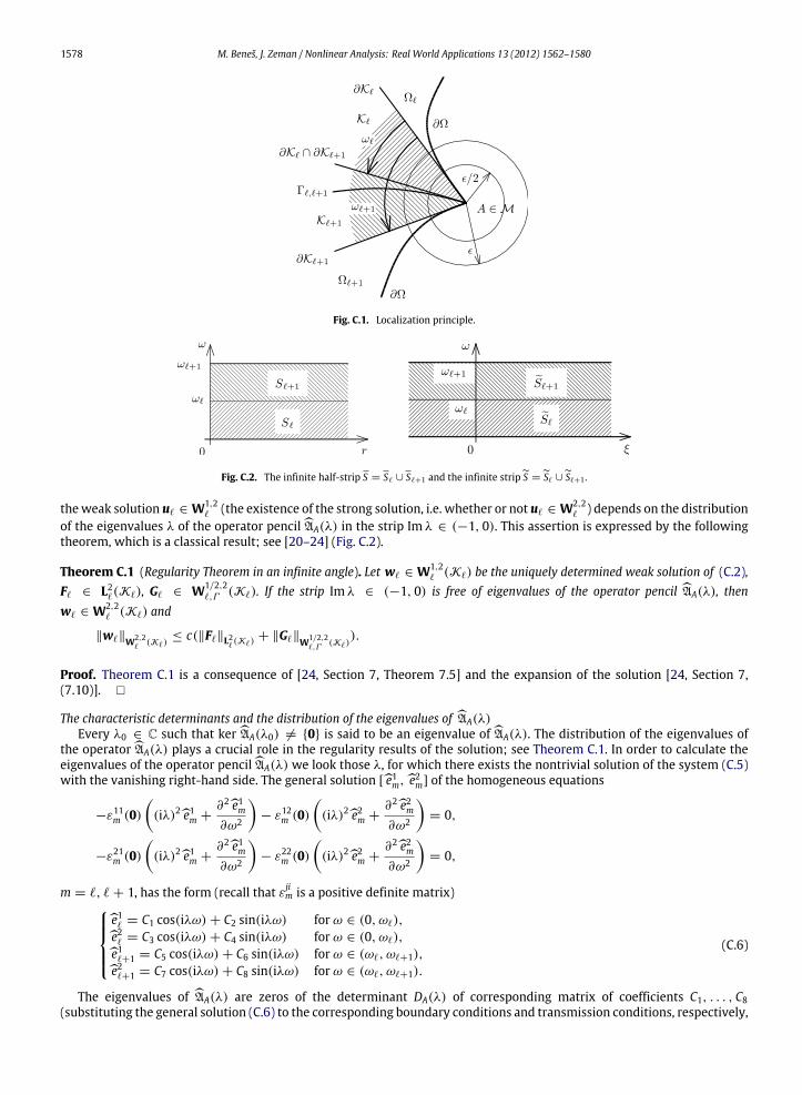
Fig. C.1. Localization principle.

Fig. C.2. The infinite half-strip S = Sℓ ∪ Sℓ+1 and the infinite stripS =Sℓ ∪Sℓ+1 .

theweak solution uℓ ∈ W1,2ℓ (the existence of the strong solution, i.e. whether or not uℓ ∈ W2,2

ℓ ) depends on the distributionof the eigenvalues λ of the operator pencilAA(λ) in the strip Im λ ∈ (−1, 0). This assertion is expressed by the followingtheorem, which is a classical result; see [20–24] (Fig. C.2).

Theorem C.1 (Regularity Theorem in an infinite angle). Let wℓ ∈ W1,2ℓ (Kℓ) be the uniquely determined weak solution of (C.2),

Fℓ ∈ L2ℓ(Kℓ), Gℓ ∈ W1/2,2ℓ,Γ (Kℓ). If the strip Im λ ∈ (−1, 0) is free of eigenvalues of the operator pencil AA(λ), then

wℓ ∈ W2,2ℓ (Kℓ) and

∥wℓ∥W2,2ℓ

(Kℓ)≤ c(∥Fℓ∥L2

ℓ(Kℓ)

+ ∥Gℓ∥W1/2,2ℓ,Γ

(Kℓ)).

Proof. Theorem C.1 is a consequence of [24, Section 7, Theorem 7.5] and the expansion of the solution [24, Section 7,(7.10)].

The characteristic determinants and the distribution of the eigenvalues of AA(λ)Every λ0 ∈ C such that ker AA(λ0) = 0 is said to be an eigenvalue of AA(λ). The distribution of the eigenvalues of

the operatorAA(λ) plays a crucial role in the regularity results of the solution; see Theorem C.1. In order to calculate theeigenvalues of the operator pencilAA(λ) we look those λ, for which there exists the nontrivial solution of the system (C.5)with the vanishing right-hand side. The general solution [e1m,e2m] of the homogeneous equations

−ε11m (0)

(iλ)2e1m +

∂2e1m∂ω2

− ε12

m (0)

(iλ)2e2m +∂2e2m∂ω2

= 0,

−ε21m (0)

(iλ)2e1m +

∂2e1m∂ω2

− ε22

m (0)

(iλ)2e2m +∂2e2m∂ω2

= 0,

m = ℓ, ℓ + 1, has the form (recall that εjim is a positive definite matrix)

e1ℓ = C1 cos(iλω) + C2 sin(iλω) for ω ∈ (0, ωℓ),e2ℓ = C3 cos(iλω) + C4 sin(iλω) for ω ∈ (0, ωℓ),e1ℓ+1 = C5 cos(iλω) + C6 sin(iλω) for ω ∈ (ωℓ, ωℓ+1),e2ℓ+1 = C7 cos(iλω) + C8 sin(iλω) for ω ∈ (ωℓ, ωℓ+1).

(C.6)

The eigenvalues of AA(λ) are zeros of the determinant DA(λ) of corresponding matrix of coefficients C1, . . . , C8(substituting the general solution (C.6) to the corresponding boundary conditions and transmission conditions, respectively,


we get the homogeneous linear system of eight equations with unknowns C1, . . . , C8). Computation of DA(λ) leads to thetranscendent equation

DA(λ) = D11A (λ)D22

A (λ) − D12A (λ)D21

A (λ) = 0, (C.7)

where

D11A (λ) = ε11

ℓ (0) sin(iλωℓ) cos[iλ(ωℓ+1 − ωℓ)] + ε11ℓ+1(0) cos(iλωℓ) sin[iλ(ωℓ+1 − ωℓ)],

D12A (λ) = ε12


D21A (λ) = ε21


D22A (λ) = ε22

ℓ (0) sin(iλωℓ) cos[iλ(ωℓ+1 − ωℓ)] + ε22ℓ+1(0) cos(iλωℓ) sin[iλ(ωℓ+1 − ωℓ)].

The roots of the equation DA(λ) = 0 are the eigenvalues ofAA(λ).Taking into account the special type of geometry, namely ωℓ = ωℓ+1/2, (C.7) simplifies into

12[(ε11

ℓ (0) + ε11ℓ+1(0))(ε

22ℓ (0) + ε22

ℓ+1(0)) − (ε12ℓ (0) + ε12

ℓ+1(0))(ε21ℓ (0) + ε21

ℓ+1(0))] sin(2iλωℓ) = 0. (C.8)

Since both matrices, εijℓ and ε

ijℓ+1, are considered to be positive definite, we get

sin(2iλωℓ) = 0, (C.9)

from whence we obtain

iλ =kπ2ωℓ

, k ∈ Z.

Now it is clear that for ωℓ ∈ (0, π/2] there are no roots of the equation DA(λ) = 0 such that Im λ ∈ (−1, 0).

Corollary 1. Let uℓ ∈ W1,2ℓ be the uniquely determined weak solution of (C.1), fℓ ∈ L2ℓ , gℓ ∈ W1/2,2

ℓ,Γ . Since the stripIm λ ∈ (−1, 0) is free of eigenvalues of the operator AA(λ), we have uℓ ∈ W2,2

ℓ and

∥uℓ∥W2,2ℓ

≤ c(∥fℓ∥L2ℓ+ ∥gℓ∥W1/2,2

ℓ,Γ

).

Sketch of the Proof. The assertion follows from Theorem C.1 and the determinant equation (C.7). (C.7) implies that forωℓ+1 ≤ π , ωℓ = ωℓ+1/2 there are no eigenvalues of the operatorAA(λ) in the strip Im λ ∈ (−1, 0). Hence wℓ ∈ W2,2

ℓ (Kℓ).Now consider the weak solution uℓ ∈ W1,2

ℓ of (C.1). Let Mℓ be the set of all boundary corner points A ∈ ∂Ωℓ, ℓ = 1, . . . ,M .We have

uℓ =

1 −

A∈Mℓ

ηA

uℓ +

A∈Mℓ

ηAuℓ (C.10)

=

1 −

A∈Mℓ

ηA

uℓ +

A∈Mℓ

wℓ. (C.11)

The regularity of the first term on the right-hand side follows from the interior regularity. The smoothness of the secondterm follows from the regularity result in an infinite angle Kℓ, Theorem C.1.

References

[1] R. Černý, P. Rovnaníková, Transport Processes in Concrete, Spon Press, 2002.[2] H.S.L.C. Hens, Modeling the heat, air, and moisture response of building envelopes: What material properties are needed, how trustful are the

predictions? J. ASTM Int. 4 (2007) 1–11.[3] A. Kalagasidis, P. Weitzmann, T. Nielsen, R. Peuhkuri, C. Hagentoft, C. Rode, The international building physics toolbox in Simulink, Energy Build. 39

(2007) 665–674.[4] H.W. Alt, S. Luckhaus, Quasilinear elliptic-parabolic differential equations, Math. Z. 183 (1983) 311–341.[5] J. Filo, J. Kačur, Local existence of general nonlinear parabolic systems, Nonlinear Anal. 24 (1995) 1597–1618.[6] J. Vala, On a system of equations of evolution with a non-symmetrical parabolic part occuring in the analysis of moisture and heat transfer in porous

media, Appl. Math. 47 (2002) 187–214.[7] B. Li, W. Sun, Global existence of weak solution for nonisothermal multicomponent flow in porous textile media, SIAM J. Math. Anal. 42 (2010)

3076–3102.[8] B. Li, W. Sun, Y. Wang, Global existence of weak solution to the heat and moisture transport system in fibrous porous media, J. Differential Equations

249 (2010) 2618–2642.[9] M. Giaquinta, G. Modica, Local existence for quasilinear parabolic systems under nonlinear boundary conditions, Ann. Mat. Pura Appl. 149 (1987)

41–59.


[10] P. Weidemaier, Local existence for parabolic problems with fully nonlinear boundary condition; an Lp-approach., Ann. Mat. Pura Appl. 160 (1991)207–222.

[11] A. Adams, J.F. Fournier, Sobolev spaces, in: Pure and Applied Mathematics, vol. 140, Academic Press, 1992.[12] A. Kufner, O. John, S. Fučík, Function Spaces, Academia, 1977.[13] J. Dalík, J. Daněček, S Št’astník, A model of simultaneous distribution of moisture and temperature in porous materials, Ceram. -Silik. 41 (1997) 41–46.[14] K. Kiessl, Kapillarer und dampfförmiger Feuchtetransport in mehrshichtigen Bauteilen. Rechnerische Erfassung und bauhysikalische Anwendung,

Dissertation, Universität Essen, 1983.[15] H.M. Künzel, Simultaneous heat and moisture transport in building components: one- and two-dimensional calculation using simple parameters,

Ph.D. Thesis, Fraunhofer Institute of Building Physics, 1995.[16] H.M. Künzel, K. Kiessl, Calculation of heat and moisture transfer in exposed building components, Int. J. Heat Mass. Transfer. 40 (1997) 159–167.[17] J. Dalík, J. Daněček, J Vala, Numerical solution of the Kiessl model, Appl. Math. 45 (2000) 3–17.[18] T. Roubíček, Nonlinear Partial Differential Equations With Applications, Birkhäuser, 2005.[19] N.M. Hung, N.T. Anh, Regularity of solutions of initial-boundary value problems for parabolic equations in domains with conical points, J. Differential

Equations 245 (2008) 1801–1818.[20] M. Dauge, Elliptic Boundary Value Problems on Corner Domains: Smoothness and Asymptotics of Solutions, in: Lecture Notes in Mathematics,

vol. 1341, Springer, 1988.[21] V.A. Kondra’tev, Boundary value problems for elliptic equations on domains with conical or angular points, Trudy Moskov. Mat. Obshch. 16 (1967)

(in Russian).[22] V.A. Kozlov, V.G. Mazya, J. Rossmann, Elliptic Boundary Value Problems with Point Singularities, American Mathematical Society, 1997.[23] V.A. Kozlov, V.G.Mazya, J. Rossmann, Spectral problems associatedwith corner singularities of solutions to elliptic equations, in:Mathematical Surveys

and Monographs, vol. 85, American Mathematical Society, 2001.[24] A. Kufner, A.M. Sändig, Some Aplications ofWeighted Sobolev Spaces, in: Teubner-Texte zur Mathematik, vol. 100, Teubner Verlagsgesellschaft, 1987.[25] S. Nicaise, A.M. Sändig, General interface problems I, Math. Methods Appl. Sci. 17 (1994) 395–429.[26] S. Nicaise, A.M. Sändig, General interface problems II, Math. Methods Appl. Sci. 17 (1994) 431–450.[27] A.M. Sändig, Stress singularities in composites, in: Multifield problems, vols. 270–277, Springer-Verlag, 2000.

some properties of strong solutions to nonlinear heat and moisture transport in multi-layer porous...

Documents