some practical issues applying mixed longitudinal...

Some practical issues applying

mixed longitudinal models for observational data Georges Monette With help from: Pauline Wong, Tammy Kostecki-Dillon, Yifaht Korman, Qing Shao, Alina Rivilis, Ernest Kwan

1

X

Y

Subj 1

Subj 2

Subj 3

Subj 4

Example: 4 subjects each observed at 3 dosages

2

Model for ith patient on jth occasion: (Subject-level model)

20 1 iid N(0, )ij ij ii j ijiY X ε σβ β ε= + +

Some possible models (not all very sensible):

Population model Splus notationFixed effects

1

0

1

i

i

ββ

free parameters

γ=

Y ~ X + Subj

Random effects 0 00

1

iid N( , )γ τ0

1

i

i

ββ γ=

Y ~ X, Random = ~ 1 | Subj

Marginal model (pooled, ignore subjects)

Y ~ X

0

1

i

i

ββ 1

γγ0=

=

3

Y

X

iβ0

1i

β

4

X

Y

iβ0

1i

β

Hypothetical intercept and slope for Subject i = 2

4

Marginal Model (Pooled Data): Ignore Subjects + Regress

2

0 iid N(0, )ij ij ij ijY Xγ γ ε ε σ1= + +

Y ~ X

5

X

Y

Marginal Model (Pooled Data): Ignore Subjects + Regress

6

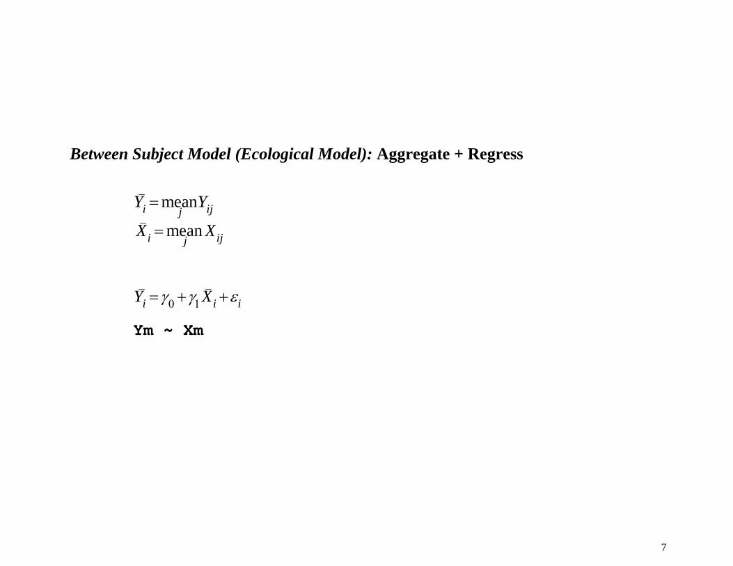
Between Subject Model (Ecological Model): Aggregate + Regress

meani ijjY Y=

meani ijjX X=

i i iY Xγ γ ε0 1= + +

Ym ~ Xm

7

X

Y

Between Subject Model (Ecological Model): Aggregate + Regress

8

Within Subjects Model (Fixed Effects):

20 1 iid N(0, )ij ij ii j ijiY X ε σβ β ε= + +

Y ~ X + Subj

9

X

Y

Within Subjects Model (Fixed Effects)

10

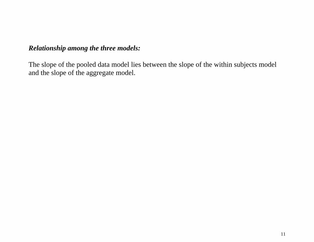
Relationship among the three models: The slope of the pooled data model lies between the slope of the within subjects model and the slope of the aggregate model.

11

X

Y

X

Y

X

Y

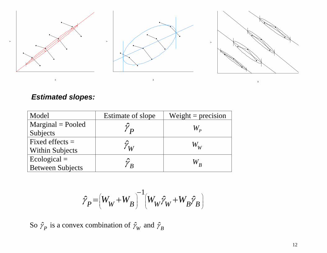
Estimated slopes: Model Estimate of slope Weight = precision Marginal = Pooled Subjects

ˆPγ PW

Fixed effects = Within Subjects Wγ WW

Ecological = Between Subjects

ˆBγ BW

1ˆ ˆ ˆP W B W W B BW W W Wγ γ γ⎛ ⎞ ⎛ ⎞

⎜ ⎟ ⎜ ⎟⎜ ⎟ ⎜ ⎟⎝ ⎠ ⎝ ⎠

−= + +

So ˆPγ is a convex combination of Wγ and ˆBγ

12

Q: What is ˆMMγ , the slope of the random effects model? A: A different convex combination of Wγ and ˆBγ .

Estimate Weight

Wγ WW

ˆBγ Bn W

nσ

τ σ2

200 +

( ) 1ˆ ˆ ˆB B W Wn W W

nσγ γ γ

τ σ

⎡ ⎤⎢ ⎥⎢ ⎥⎢ ⎥⎣ ⎦

2−ΜΜ 2

00= × +

+

13

So: If n

στ2

00× is small then ˆ ˆMM Wγ γ≈

If n

στ2

00× is big then ˆ ˆMM Pγ γ≈

So the random effects model seems ok if n (number of observations within Subjects) is large of if the variation within subjects is small compared to variation between Subjects.

14

X

Y

X

Y

X

Y

X

Y

15

In passing: The fact that Wγ and ˆPγ can have opposite signs is Simpson’s (Yule’s) Paradox The fact that Wγ and ˆBγ can have opposite signs is Robinson’s Paradox

16

Fixed effects vs. random effects:

pluses minusesFixed effects Within Subject effect not

biased by different between Subject relationship

-Hard to model between Subject effects -Inference generalizes to new observations on same Subjs

Random effects

- Can include other between Subj variables and within Subj variables - Inference generalizes to population of Subjs

- Unless effects between S and within S are the same, estimate of within S effect is biased

17

Getting the best of both worlds: Adjust for contextual effects using random effects + contextual effect.

- Within Subject estimate is not biased by between subject effect. - Can include other between S effects - Inference for random effects generalizes to larger population

i.e. we don’t need to fully control for Subjs as in fixed effects models, only for the ‘configuration’ of within Ss effects.

18

Model with a contextual effect of X:

meani ijjX X=

( ) 20 iid N(0, ) iid N( , )ij ij i i ij ijiY X X X ιβ γ γ ε ε σ β γ τ−1 2 0 0 00= + + +

Y ~ (X-Xb) + Xb, ~ 1 | Subj

Fitting this model:

1 Wγ γ= and 2ˆ ˆBγ γ=

19

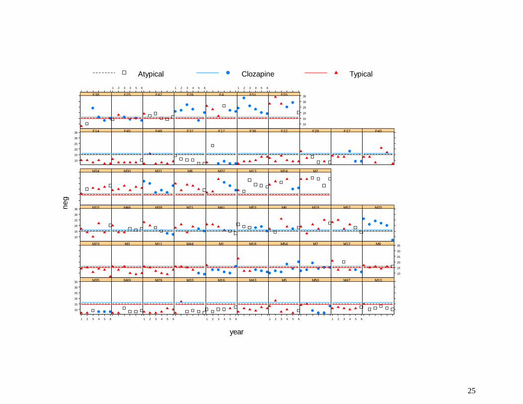
Looking at Clinical Records: 6-year study of schizophrenia patients 55 patients with schizophrenia followed for 6 years Recorded annually:

- severity of symptoms: negative, positive - drug currently prescribed: Typical, Atypical, Clozapine

20

Fraction of 330 (NA: 0 )

Dat

a

0.0 0.2 0.4 0.6 0.8 1.0

2030

4050

age1

Fraction of 330 (NA: 0 )D

ata

0.0 0.2 0.4 0.6 0.8 1.0

0.0

0.2

0.4

0.6

0.8

1.0

gender


Dat

a

0.0 0.2 0.4 0.6 0.8 1.0

010

2030

yrsill1


Dat

a

0.0 0.2 0.4 0.6 0.8 1.0

1.0

2.0

3.0

4.0

marital


Dat

a

0.0 0.2 0.4 0.6 0.8 1.0

1015

2025

30

pos


Dat

a

0.0 0.2 0.4 0.6 0.8 1.0

1015

2025

3035

neg


Dat

a0.0 0.2 0.4 0.6 0.8 1.0

4060

8010

0

total


Dat

a

0.0 0.2 0.4 0.6 0.8 1.0

12

34

56

year

35142945491643473622371023503114448193352527287424654122140415315171830343938819524620263113243225155

0 1 2 3 4 5 6

subject

Atypical

Clozapine

Typical

0 50 100 150

drug

Married

Separated/Divorced

Single

0 50 150 250

status

F

M

0 50 100 150 200

Sex

21

10

15

20

25

30

35 M35

1 2 3 4 5 6

M49 M29

1 2 3 4 5 6

M33 M16

1 2 3 4 5 6

M43 M5

1 2 3 4 5 6

M50 M47

1 2 3 4 5 6

M10

M23 M3 M11 M44 M1 M18 M54 M7 M12

10

15

20

25

30

35M9

10

15

20

25

30

35 M15 M46 M39 M21 M41 M53 M6 M19 M52 M20

M34 M30 M31 M8 M32 M13 M24 M2

10

15

20

25

30

35 F14 F45 F48 F37 F17 F36 F22 F28 F27 F40

F38 F25

1 2 3 4 5 6

F42 F26

1 2 3 4 5 6

F4 F51

1 2 3 4 5 6

10

15

20

25

30

35F55

year

neg

22

10

15

20

25

30

35 M35

1 2 3 4 5 6

M49 M29

1 2 3 4 5 6

M33 M16

1 2 3 4 5 6

M43 M5

1 2 3 4 5 6

M50 M47

1 2 3 4 5 6

M10

M23 M3 M11 M44 M1 M18 M54 M7 M12

10

15

20

25

30

35M9

10

15

20

25

30

35 M15 M46 M39 M21 M41 M53 M6 M19 M52 M20

M34 M30 M31 M8 M32 M13 M24 M2

10

15

20

25

30

35 F14 F45 F48 F37 F17 F36 F22 F28 F27 F40

F38 F25

1 2 3 4 5 6

F42 F26

1 2 3 4 5 6

F4 F51

1 2 3 4 5 6

10

15

20

25

30

35F55

year

neg

Atypical Clozapine Typical

23

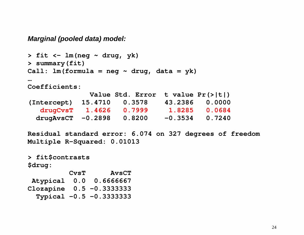
Marginal (pooled data) model: > fit <- lm(neg ~ drug, yk) > summary(fit) Call: lm(formula = neg ~ drug, data = yk) … Coefficients: Value Std. Error t value Pr(>|t|) (Intercept) 15.4710 0.3578 43.2386 0.0000 drugCvsT 1.4626 0.7999 1.8285 0.0684 drugAvsCT -0.2898 0.8200 -0.3534 0.7240 Residual standard error: 6.074 on 327 degrees of freedom Multiple R-Squared: 0.01013 > fit$contrasts $drug: CvsT AvsCT Atypical 0.0 0.6666667 Clozapine 0.5 -0.3333333 Typical -0.5 -0.3333333

24

10

15

20

25

30

35 M35

1 2 3 4 5 6

M49 M29

1 2 3 4 5 6

M33 M16

1 2 3 4 5 6

M43 M5

1 2 3 4 5 6

M50 M47

1 2 3 4 5 6

M10

M23 M3 M11 M44 M1 M18 M54 M7 M12

10

15

20

25

30

35M9

10

15

20

25

30

35 M15 M46 M39 M21 M41 M53 M6 M19 M52 M20

M34 M30 M31 M8 M32 M13 M24 M2

10

15

20

25

30

35 F14 F45 F48 F37 F17 F36 F22 F28 F27 F40

F38 F25

1 2 3 4 5 6

F42 F26

1 2 3 4 5 6

F4 F51

1 2 3 4 5 6

10

15

20

25

30

35F55

year

neg


25

10

15

20

25

30

35 M5

1 2 3 4 5 6

M50 M8

1 2 3 4 5 6

F4 F51

1 2 3 4 5 6

10

15

20

25

30

35F55

year

neg


26 26

Fixed effects model > fit <- lm(neg ~ Subject + drug, yk) > summary(fit) Call: lm(formula = neg ~ Subject + drug, data = yk) . . . Coefficients: Value Std. Error t value Pr(>|t|) (Intercept) 15.0224 0.2101 71.5066 0.0000 Subject^1 18.4655 1.4198 13.0060 0.0000 Subject^2 -10.1621 1.3952 -7.2834 0.0000 . . . . Subject^54 -0.9233 1.4519 -0.6360 0.5253 drugCvsT -2.6789 0.7126 -3.7591 0.0002 drugAvsCT 0.4427 0.6432 0.6883 0.4919 Residual standard error: 3.383 on 273 degrees of freedom Multiple R-Squared: 0.7436 F-statistic: 14.14 on 56 and 273 degrees of freedom, the p-

value is 0

27


10

15

20

25

30

35 M5

1 2 3 4 5 6

M50 M8

F4 F51

1 2 3 4 5 6

F55

20

30

35

25

15

10

gne

1 2 3 4 5 6

year

28

Random Effects Model

> fit <- lme(neg ~ drug, yk, random = ~ 1 | Subject) > summary(fit) Linear mixed-effects model fit by REML Data: yk AIC BIC logLik 1896.737 1915.687 -943.3684 Random effects: Formula: ~ 1 | Subject (Intercept) Residual StdDev: 5.285956 3.38706 Fixed effects: neg ~ drug Value Std.Error DF t-value p-value (Intercept) 15.08599 0.7427055 273 20.31222 <.0001 drugCvsT -2.06226 0.6795131 273 -3.03491 0.0026 drugAvsCT 0.26296 0.6230209 273 0.42208 0.6733 . . .

29


10

15

20

25

30

35 M5

1 2 3 4 5 6

M50 M8

1 2 3 4 5 6

F4 F51

1 2 3 4 5 6

10

15

20

25

30

35F55

neg

year

30

Creating contextual variables

> zm <- model.matrix(~drug, data=yk) > summ <- function( x, id ,to = id) tapply( x, id, mean) [

tapply(to, to) ] > yk$D1 <- summ( zm[,2], yk$Subject ) > yk$D2 <- summ( zm[,3], yk$Subject ) > z <- yk[match(yk$Subject,c("M5","F51"),0)>0,

c('Subject','drug','D1','D2')]

31

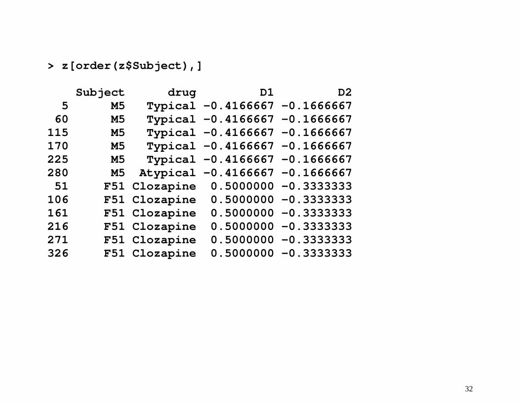
> z[order(z$Subject),]

D2

7 al -0.4166667 -0.1666667 66667 66667

271 F51 Clozapine 0.5000000 -0.3333333 326 F51 Clozapine 0.5000000 -0.3333333

Subject drug D1 5 M5 Typical -0.4166667 -0.1666667 60 M5 Typical -0.4166667 -0.1666667 115 M5 Typical -0.4166667 -0.1666667 0 M5 Typic1

225 M5 Typical -0.4166667 -0.16280 M5 Atypical -0.4166667 -0.16 51 F51 Clozapine 0.5000000 -0.3333333 106 F51 Clozapine 0.5000000 -0.3333333 161 F51 Clozapine 0.5000000 -0.3333333 216 F51 Clozapine 0.5000000 -0.3333333

32

Random effects with contextual variables

e p-value 5 <.0001

drugAvsCT 0.44267 0.643161 273 0.68828 0.4919 D1 7.02777 2.277980 52 3.08509 0.0033 D2 -0.12883 2.586383 52 -0.04981 0.9605 . . .

> fit <- lme(neg ~ drug + D1 + D2, yk, random = ~ 1 | subject) > summary(fit) . . . Random effects: Formula: ~ 1 | subject (Intercept) Residual StdDev: 4.954323 3.383306 Fixed effects: neg ~ drug + D1 + D2 Value Std.Error DF t-valu(Intercept) 15.90782 0.800017 273 19.8843 drugCvsT -2.67886 0.712639 273 -3.75907 0.0002

33


10

15

20

25

30

35 M5

1 2 3 4 5 6

M50 M8

F4 F51

1 2 3 4 5 6

10

15

20

25

30

35F55

neg

1 2 3 4 5 6

year

34

Random effects with contextual variables + year > fit <- lme(neg ~ D1 + D2 + year + drug, yk, random = ~ 1 | Subject) > summary(fit) . . . Random effects: Formula: ~ 1 | Subject (Intercept) Residual StdDev: 4.96086 3.325338 Fixed effects: neg ~ D1 + D2 + year + drug Value Std.Error DF t-value p-value (Intercept) 17.41323 0.924015 272 18.84517 <.0001 D1 5.54906 2.319095 52 2.39277 0.0204 D2 -0.30206 2.584212 52 -0.11689 0.9074 year -0.43012 0.132103 272 -3.25592 0.0013 drugCvsT -1.20014 0.834784 272 -1.43767 0.1517 drugAvsCT 0.61591 0.634376 272 0.97088 0.3325 . . .

35

Atypical Clozapine Typical1 2 3 4 5 6

10

15

20

25

30

35 M5

1 2 3 4 5 6

M50 M8

F4 F51

10

15

20

25

30

35F55

1 2 3 4 5 6

year

neg

36

A related article on multilevel modeling and measurement error: Schwartz & Coull (2003). Also:

Schwartz, J., & Coull, B. A. (2003). Control for confounding in the presence of measurement error in hierarchical models. Biostatistics, 4(4), 539-553.

37

some practical issues applying mixed longitudinal...

Documents