some new improvements of jensen’s inequality
TRANSCRIPT

MONOGRAPHS IN INEQUALITIES 19
Some New Improvements of Jensen’s Inequality
Jensen’s Type Inequalities in Information Theory
Muhammad Adil Khan, Khuram Ali Khan, Dilda Pecaric and Josip Pecaric


Some New Improvementsof Jensen’s Inequality
Jensen’s Type Inequalitiesin Information Theory
Muhammad Adil Khan
Department of Mathematics
University of Peshawar, Peshawar, Pakistan
Khuram Ali Khan
Department of Mathematics
University of Sargodha, Sargodha, Pakistan
Dilda Pecaric
Catholic University of Croatia
Zagreb, Croatia
Josip Pecaric
RUDN University
Moscow, Russia.
Zagreb, 2020

MONOGRAPHS IN INEQUALITIES 19
Some New Improvements of Jensen’s Inequality
Jensen’s Type Inequalities in Information Theory
Muhammad Adil Khan, Khuram Ali Khan, Dilda Pecaric and JosipPecaric
Neda Lovricevic
Faculty of Civil Engineering, Architecture and GeodesyUniversity of SplitSplit, Croatia
Julije Jaksetic
Department of MathematicsFaculty of Mechanical Engineeringand Naval ArchitectureUniversity of ZagrebZagreb, Croatia
1st edition
Copyright c© by Element, Zagreb, 2020.
Printed in Croatia.All rights reserved.
A CIP catalogue record for this book is available from the National andUniversity Library in Zagreb under 001063424.
ISBN 978-953-197-689-3
No part of this publication may be reproduced or distributed in any formor by any means, or stored in a data base or retrieval system, withoutthe prior written permission of the publisher.

Preface
The classical Jensen inequality is a famous tool to construct new results in the theoryof inequalities. It has numerous applications in abstract and applied sciences. In thismonograph, some recent developments in theory of inequalities with respect to Jensen’sinequality are collected and presented. Applications are given in information theory byevaluating the estimates for different entropies and divergences via some recent and exist-ing refinements of Jensen’s inequality. The results for convex functions in this context arealso generalized for higher order convex functions by means of interpolating polynomials.
In the first chapter, some basic notions and preliminary results are recalled which areused in the sequel.
In the second chapter, we focus on the refinements of integral Jensen’s as well as dis-crete Jensen’s inequalities. First we derive a refinement of integral Jensen’s inequalityassociated to two functions whose sum is equal to unity. As applications of the refinementof integral Jensen’s inequality we obtain refinements of Holder, integral power means andHermite-Hadamard inequalities. We also give applications in information theory and pro-vide a more general refinement of integral Jensen’s inequality. We establish a refinementof discrete Jensen’s inequality concerning certain tuples and give applications to differentmeans. Finally, we give applications of discrete main result in information theory andprovide a more general refinement of discrete Jensen’s inequality.
In the third chapter, we derive refinements of discrete as well as integral Jensen-Steffensen’s inequalities associated to certain tuples and functions respectively and alsopresent application to the Zipf Mandelbrot law. Some more general refinements are alsopresented for Jensen-Steffensen’s inequality.
In the fourth chapter, we propose new refinements for the Jensen-Mercer as well asfor variant of the Jensen-Mercer inequalities associated to certain positive tuples. We givesome related integral versions and present applications for different means. Further gener-alizations are given which are associated to m finite sequences.
In the fifth chapter, we give a refinement of Jensen’s inequality for convex functionsof several variables associated to certain tuples. As an application, we deduce refinementsof Beck’s inequality. At the end, further generalization has been presented for n finitesequences.
In the sixth chapter, we present refinements of generalized Jensen’s inequalities givenby Jessen and McShane. As applications of the refinement of Jessen’s inequality, we de-duce refinements of generalized means and Holder inequalities. Also, as applications ofthe refinement of McShane’s inequality, we obtain refinements of generalized Beck’s in-
v

equality and discuss their particular cases. At the end of this chapter, we give furthergeneralizations of Jessen’s and McShane’s inequalities pertaining n certain functions.
In the seventh chapter, we obtain a refinement of Jensen’s inequality for operator con-vex functions. Some applications are presented for different means and also, deducedrefinement of operator inequality connected to the operator concavity of operator entropyA logA−1. Further generalization is also given for operator Jensen’s inequality.
In the eighth chapter, estimation of f -divergence, Shannon entropy, Renyi divergenceand Renyi entropy are studied via refinements of Jensen’s inequality. The results show theapplications of Jensen’s inequality in information theory.
In the ninth chapter, Montgomery identity, Hermite interpolation, Lidstone polyno-mial, Fink identity and Abel-Gontscharoff Green function, Taylor one point and Taylortwo point formula are used to generalize the refinements of Jensen, Renyi and Shannontype inequalities for the class of higher order convex functions.
In the tenth chapter, an integral form of Popoviciu’s inequality involving samples withrepetitions and without repetitions is given with the refinement of the integral Jensen in-equality. Applications to power means are studied with respect to monotonicity property.
In the eleventh chapter, the Jensen differences involving two types of data points arerefined for the class of 3-convex functions.
Authors
vi

Contents
Preface v
1 Introduction 11.1 Some Inequalities Involving Convex Functions . . . . . . . . . . . . . . 1
1.1.1 J-Convex Functions . . . . . . . . . . . . . . . . . . . . . . . . . 21.1.2 Convex Functions . . . . . . . . . . . . . . . . . . . . . . . . . . 21.1.3 Operator Convex Functions . . . . . . . . . . . . . . . . . . . . 21.1.4 Discrete Jensen’s Inequality . . . . . . . . . . . . . . . . . . . . 21.1.5 Discrete Jensen-Steffensen’s Inequality . . . . . . . . . . . . . . 31.1.6 Integral Form of Jensen’s Inequality . . . . . . . . . . . . . . . . 31.1.7 Integral Version of Jesnen-Steffensen’s Inequality . . . . . . . . . 31.1.8 Jensen-Mercer’s Inequality . . . . . . . . . . . . . . . . . . . . . 71.1.9 Variant of Jensen-Steffensen’s Inequality . . . . . . . . . . . . . 71.1.10 Jensen’s Inequality for Operator Convex Functions . . . . . . . . 71.1.11 Hermite-Hadamard Inequality . . . . . . . . . . . . . . . . . . . 81.1.12 Holder Inequality . . . . . . . . . . . . . . . . . . . . . . . . . . 8
1.2 Power Means . . . . . . . . . . . . . . . . . . . . . . . . . . . . . . . . 81.2.1 Quasi-Arithmetic Means . . . . . . . . . . . . . . . . . . . . . . 9
1.3 Divided Differences . . . . . . . . . . . . . . . . . . . . . . . . . . . . . 101.4 Higher Order Convex Functions . . . . . . . . . . . . . . . . . . . . . . 101.5 Information Divergence Measures and Entropies . . . . . . . . . . . . . . 11
1.5.1 Zipf-Mandelbrot Law . . . . . . . . . . . . . . . . . . . . . . . . 13
2 Refinements of Jensen’s Inequality 152.1 Refinement of Integral Jensen’s Inequality . . . . . . . . . . . . . . . . . 15
2.1.1 Applications in Information Theory . . . . . . . . . . . . . . . . 202.1.2 Further Generalization . . . . . . . . . . . . . . . . . . . . . . . 23
2.2 Refinement of Discrete Jensen’s Inequality . . . . . . . . . . . . . . . . . 242.2.1 Applications in Information Theory . . . . . . . . . . . . . . . . 262.2.2 Further Generalization . . . . . . . . . . . . . . . . . . . . . . . 30
3 Refinements of Jensen-Steffensen’s Inequality 313.1 Refinements of Jensen-Steffensen’s Inequality . . . . . . . . . . . . . . . 313.2 Further Generalization . . . . . . . . . . . . . . . . . . . . . . . . . . . 34
vii

4 Refinements of Jensen-Mercer’s and Variant of Jensen-Steffensen’sInequalities 374.1 Refinements . . . . . . . . . . . . . . . . . . . . . . . . . . . . . . . . . 374.2 Applications to Means . . . . . . . . . . . . . . . . . . . . . . . . . . . 404.3 Further Generalizations . . . . . . . . . . . . . . . . . . . . . . . . . . . 42
5 Refinement of Jensen’s Inequality for Convex Functions of SeveralVariables 455.1 Refinement of Jensen’s Inequality for Convex Functions of Several
Variables with Applications . . . . . . . . . . . . . . . . . . . . . . . . . 455.2 Further Generalization . . . . . . . . . . . . . . . . . . . . . . . . . . . 51
6 Refinements of Jessen’s and McShane’s Inequalities 556.1 Refinement of Jessen’s Inequality with Applications . . . . . . . . . . . . 556.2 Refinement of McShane’s Inequality with Applications . . . . . . . . . . 606.3 Further Generalizations . . . . . . . . . . . . . . . . . . . . . . . . . . . 63
7 Refinement of Jensen’s Operator Inequality 677.1 Refinement of Jensen’s Operator Inequality with Applications . . . . . . 677.2 Further Generalization . . . . . . . . . . . . . . . . . . . . . . . . . . . 72
8 Estimation of Different Entropies and Divergences via Refinementof Jensen’s Inequality 738.1 Estimation of Csiszar Divergence . . . . . . . . . . . . . . . . . . . . . . 738.2 Estimation of Shannon Entropy . . . . . . . . . . . . . . . . . . . . . . . 758.3 Estimation of Kullback-Leibler Divergence . . . . . . . . . . . . . . . . 768.4 Inequalities for Renyi Divergence and Entropy . . . . . . . . . . . . . . . 778.5 Relation Between Shannon Entropy and Divergence . . . . . . . . . . . . 818.6 Inequalities by Using Zipf-Mandelbrot Law . . . . . . . . . . . . . . . . 838.7 Relation Between Shannon Entropy and Zipf-Mandelbrot Law . . . . . . 848.8 Relation Between Shannon Entropy and Hybrid Zipf-Mandelbrot Law . . 85
9 Divergence and Entropy Results via Interpolating Polynomialsfor m-convex Function 879.1 New Generalized Functionals . . . . . . . . . . . . . . . . . . . . . . . . 879.2 Generalization of Refinement of Jensen’s, Renyi and Shannon
Type Inequalities via Montgomery Identity . . . . . . . . . . . . . . . . . 909.3 Generalization of Refinement of Jensen’s, f-divergence, Shannon
and Renyi type Inequalities via Hermite Interpolating Polynomial . . . . 939.4 Generalization of Refinement of Jensen’s, Renyi and Shannon
Type Inequalities via Lidstone Polynomial . . . . . . . . . . . . . . . . . 1009.5 Generalization of Refinement of Jensen’s, Renyi and Shannon
Type Inequalities via Fink Identity and Abel-GontscharoffGreen Fuction . . . . . . . . . . . . . . . . . . . . . . . . . . . . . . . . 102
9.6 Generalization of Refinement of Jensen’s, Renyi and Shannontype Inequalities via Taylor’s one and two point Polynomials . . . . . . . 106
viii

9.7 Bounds for the Identities Related to Generalization of Refinementof Jensen’s Inequality . . . . . . . . . . . . . . . . . . . . . . . . . . . . 110
10 Integral form of Popoviciu’s Inequality for Convex Functions 11510.1 Integral form of Popoviciu’s Inequality . . . . . . . . . . . . . . . . . . . 11510.2 New Refinement of the Integral form of Jensen’s Inequality . . . . . . . . 11810.3 New Quasi-Arithmetic Means . . . . . . . . . . . . . . . . . . . . . . . 121
11 Refinement of Jensen’s Inequality for 3-convex Functions 12311.1 Refinement of Jensen’s Inequality for 3-convex Functions at a Point . . . 123
Bibliography 131
Index 137
ix


Chapter1
Introduction
Convex functions have a significant role while dealing with optimization problems. Geom-etry of convex functions leads to many important inequalities which are frequently used toestimate and compare the values related to many physical problems in different branchesof mathematics and physics. Entropies and divergences are widely studied in informa-tion theory. While dealing with many physical problems physicist have to deal with thestructure involving higher dimension convexity. Therefore there are two important gapsfirst to estimate the entropies and divergences and second one is to study the inequalitiesfor higher dimension problems. Therefore we estimate different entropies and divergencesand secondly we generalize the related results for higher order convex functions.It is of great interest for researchers to study inequalities of continuous data and arbitraryweights. For example integral version of Popoviciu’s inequality are studied in the sequel.
1.1 Some Inequalities Involving Convex Functions
The first chapter contains: introduction to convex functions, various inequalities involvingconvex functions, refinement of these inequalities given by various researchers in recentyears, the weighted version of Popoviciu’s inequality, some notions from information the-ory containing entropies and divergences. These will be used frequently in the followingchapters while obtaining main results.
1

2 1 INTRODUCTION
1.1.1 J-Convex Functions
In 1905–1906, J. L. W. V. Jensen began the systematic study of convex functions (see [75,p.3]).
A function : I →R is said to be J-convex or mid-convex function or convex in Jensensense on I if
(
u+ v2
)≤ (u)+ (v)
2(1.1)
holds for all u,v ∈ I.The (x) = x2 and (x) = |x| for all x ∈ R are the examples of J-convex functions.
1.1.2 Convex Functions
The notion of convex function is the generalization of J-convex function for the arbitraryweight t ∈ [0,1]. In [87, p. 1] the formal definition is given as follows.Suppose X is a real vector space, C ⊂ X is a convex set. A function : C → R is said tobe convex if
(u+(1−)v)≤ (u)+ (1−)(v),
holds for all u,v ∈C and ∈ [0,1].The (x) = x2, (x) = |x|, − logx and ex for all x ∈ R are the examples of convex
functions.
1.1.3 Operator Convex Functions
Let I be an interval of real numbers and S(I) denotes the class of all self-adjoint boundedoperators defined on complex Hilbert space H whose spectra are in I. Also, assume thatSp(A) denotes the spectrum of a bounded operator A defined on H. An operator A ∈ S(I)is said to be strictly positive if it is positive and invertible, or equivalently, Sp(A)⊂ [d1,d2]for 0 < d1 < d2.
Let : I → R be a function defined on the interval I. Then is said to be operatorconvex if is continuous and
(A1 +(1− )A2) ≤ (A1)+ (1− )(A2) (1.2)
for all A1,A2 ∈ S(I) and ∈ [0,1]. If the function − is operator convex on I, then is said to be operator concave. The function is said to be operator monotone on I if is continuous on I and A1,A2 ∈ S(I), A1 ≤ A2 (i.e. A2 −A1 is positive operator ), then(A1) ≤ (A2).
1.1.4 Discrete Jensen’s Inequality
The Jensen inequality in discrete version [87, p. 43] generalizes the notion of convexfunction. Here the function operates on the convex combination of any finite number ofpoints.

1.1 SOME INEQUALITIES INVOLVING CONVEX FUNCTIONS 3
Suppose X is a real vector space, C ⊂ X is a convex set, let : C → R be a convexfunction, 1, . . . ,n ∈ [0,1] are such that n
i=1 i = 1, and y1, . . . ,yn ∈C, then
(n
=1
y
)≤
n
=1
(y). (1.3)
In the Jensen inequality, it is natural to ask the question that is it possible to relaxthe condition of nonnegative of ( = 1,2, . . . ,n) at the expense of restricting y ( =1,2, . . . ,n) more severely. The answer of this question was given by Steffensen [96]:
1.1.5 Discrete Jensen-Steffensen’s Inequality
Let : I → R be a convex function defined on the interval I. Let y ∈ I, ∈ R
( = 1,2, . . . ,n) with = n=1 . If y1 ≤ y2 ≤ ·· · ≤ yn or y1 ≥ y2 ≥ ·· · ≥ yn and
0 ≤k
=1
≤n
=1
k = 1,2, . . . ,n,n
=1
> 0, (1.4)
then
(1
n
=1
y
)≤ 1
n
=1
(y ). (1.5)
1.1.6 Integral Form of Jensen’s Inequality
The integral form of Jensen’s inequality [47] is defined as follows.Let (X ,A,) be a probability space, consider an integrable function h : X → I. Also let : I → R be a convex function. Then
⎛⎝∫X
hd
⎞⎠ ≤∫X
◦ hd . (1.6)
1.1.7 Integral Version of Jesnen-Steffensen’s Inequality
Integral version of Jensen-Steffensen’s inequality is given by:Let I be an interval in R and g,h : [a,b] → R are integrable functions such thatg() ∈ I for all ∈ [a,b]. Also, assume that : I → R is convex function and h( ◦ g) isintegrable on [a,b]. If g is monotonic on [a,b] and h satisfies
0 ≤∫
ah()d ≤
∫ b
ah()d , ∈ [a,b],
∫ b
ah()d > 0, (1.7)
then
(∫ ba g()h()d∫ b
a h()d
)≤
∫ ba h()( ◦ g)()d∫ b
a h()d. (1.8)

4 1 INTRODUCTION
This means convex function and Jensen-type inequalities are linked to each other. In factdefinition of convex function involves inequality sign. Until now, inequalities have playeda major role in convex function development. In mathematics the role of inequalities isvery important, specially in approximation theory and analysis. The linear programmingis based on inequalities. A number of mathematicians have a keen interest in the study ofmathematical inequalities.
Jensen’s inequality is the fundamental inequality for convex function. Many classi-cal inequalities (for instance Minkowski’s inequality, Holder’s inequality etc.) and otherinequalities are the consequences of Jensen’s inequality.
L. Horvath and J. Pecaric in [49] used a refinement of discrete Jensen’s inequality toconstruct a new refinement of (1.6), which is a generalization of a result given in [25].They also gave new monotone quasi arithmetic means.
In a last few decades, many researcher papers have appeared in literature concerningthe refinement of discrete Jensen’s inequality (see [47]). However the refinement of dis-crete Jensen’s inequality has been studied more compared to the refinement of its integralversion. The researchers used the refinements of (1.3) to construct new refinements of(1.6). For instance we can see the following results [88].Suppose that f is a J-convex function on an interval J, c j ∈ J, j = 1, . . . ,n. Then
r,n ≥ r−1,n r = 1, . . . ,n−1, (1.9)
where
r,n = k,n(c1, . . . ,cn) :=1(nr
) 1≤ j1<...< jr≤n
(
1r(c j1 + . . .+ c jr)
).
For positive weights the above results are given in [84].Suppose is convex function defined on an interval J, c j ∈ J ( j = 1, ...,n).
r,n(c1, . . . ,cn,1, . . . ,n):=1(n−1
r−1
)Pn
1≤ j1<...< jr≤n
( j1+ . . .+ jr)( j1c j1+ . . .+ jr c jr
j1+ . . .+ jk
)where (1, . . . ,n) is suppose to be a positive n-tuple with r
j=1 j = Pr, then
r,n(c1, . . . ,cn,1, . . . ,n) ≥ r+1,n(c1, . . . ,cn,1, . . . ,n) n = 1, . . . ,r−1. (1.10)
J. Pecaric and D. Svrtan noted that by considering the expresssion
r,n =1(n+r−1
r−1
)Pn
1≤ j1≤...≤ jk≤n
( j1 + . . .+ jr)( j1c j1 + . . .+ jr c jr
j1 + . . .+ jr
)we have the same results
(1Pn
n
i=1
ici
)≤ . . . ≤ r+1,n ≤ r,n ≤ . . . ≤ 1,n =
1Pn
n
i=1
i(ci). (1.11)
The researchers have given the refinements of (1.3) by using different indexing sets (see[50, 48]). Like many other researchers L. Horvath and J. Pecaric gave a refinement of

1.1 SOME INEQUALITIES INVOLVING CONVEX FUNCTIONS 5
(1.3) for convex functions (see [50]). They defined some essential notions to prove therefinement given as follows:
Let X be a set, let P(X) and |X | represent the power set and number of elements of setX respectively. Let N := {0}⋃{1,2, . . .}.Suppose q ≥ 1 and r ≥ 2 are two fixed integers. Suppose
r(q) := {1, . . . ,q}r
Now letFr,s : r(q) → r−1(q) 1 ≤ s ≤ r,
Fr : r(q) → P(r−1(q)) ,
andTr : P(r(q)) → P(r−1(q)) ,
are functions defined by
Fr,s(i1, . . . , ir) := (i1, i2, . . . , is−1, is+1, . . . , ir) 1 ≤ s ≤ r,
Fr(i1, . . . , ir) :=r⋃
s=1
{Fr,s(i1, . . . , ir)},
and
Tr(I) =
{/0, I = /0;⋃(i1,...,ir)∈I
Fr(i1, . . . , ir), I �= /0.
Next for all i ∈ {1, . . . ,q} consider
r,i : {1, . . . ,q}r → N,
defined by
r,i(i1, . . . , ir) is the number of occurences of i j in (i1, . . . , ir).
For each I ∈ P(r(q)) let
I,i := (i1,...,ir)∈I
r,i(i1, . . . , ir) 1 ≤ i ≤ q.
(H1) : Let n ∈ {1,2, . . .} and m ∈ {2,3, . . .}, suppose Im ⊂ m(n) such that for all i ∈{1, . . . ,n}
Im ,i ≥ 1. (1.12)

6 1 INTRODUCTION
Introduce the set Il ⊂ l(n)(1 ≤ l ≤ m−1) inductively by
Il−1 := Tl(Il) m ≥ l ≥ 2.
Obviously the set I1is {1, . . . ,n}, by (H1) and this make certain that I1,i = 1(1 ≤ i ≤ n).From (H1) we have Il ,i ≥ 1(1 ≤ i ≤ n,m−1≥ l ≥ 1).For m ≥ l ≥ 2, and for any ( j1, . . . , jl−1) ∈ Il−1, let
HIl ( j1, . . . , jl−1) := {((i1, . . . , il),k)×{1, . . . , l}|Fl,k(i1, . . . , il) = ( j1, . . . , jl−1)}.With the help of these sets they defined the functions Im,l : Il → N(m ≥ l ≥ 1) inductivelyby
Im ,m(i1, . . . , im) := 1 (i1, . . . , im) ∈ Im;
Im ,l−1( j1, . . . , jl−1) := ((i1,...,il),k)∈HIl
( j1,..., jl−1)Im,l(i1, . . . , il).
They defined some special expressions for 1 ≤ l ≤ m, as follows
Am,l = Am,l(Im,x1, . . . ,xn, p1, . . . , pn; f ) :=(m−1)!(l−1)!
(i1,...,il)∈Il
Im,l(i1, . . . , il)
(l
j=1
pi j
Im,i j
)f
⎛⎜⎜⎜⎝lj=1
pi jIm,i j
xi j
lj=1
pi jIm,i j
⎞⎟⎟⎟⎠ (1.13)
and constructed the following new refinement of (1.3).
Theorem 1.1 Assume (H1), consider a convex function f : I → R. If c1, . . . ,cn ∈ I,
1, . . . ,n ∈ R+ such thatn
s=1s = 1, then
f
(n
s=1
scs
)≤ Am,m ≤ Am,m−1 ≤ . . . ≤ Am,2
≤ Am,1 =n
s=1
s f (cs) . (1.14)
L. Horvath and J. Pecaric proved that (1.10) is the special case of Theorem 1.1.In [25], I. Brnetic et al. gave the improvement of (1.6) as follows.
Suppose : I → R is a convex function, let : [a1,a2] → I and : [a1,a2] → R+ befunctions. Suppose 1, . . . ,n ∈ R+ with n
i=1i = 1, and
=∫ a2
a1
(t)dt,
then
(
1
∫ a2
a1
(t)(t)dt
)≤ n,n ≤ . . . ≤ k+1,n ≤ k,n . . . ≤ 1,n

1.1 SOME INEQUALITIES INVOLVING CONVEX FUNCTIONS 7
=1
∫ a2
a1
(t)((t))dt,
where
k,n =1(n−1
k−1
)k
1≤i1<...<ik≤n
k
r=1
ir
∫ a2
a1
. . .
∫ a2
a1
(k
s=1
(cis)
)
×(k
j=1i j(ci j
)k
j=1i j
)dci1dci2 . . .dcik .
1.1.8 Jensen-Mercer’s Inequality
In 2003 Mercer proved the following variant of Jensen’s inequality, which is known asJensen-Mercer’s inequality.
Theorem 1.2 ([77]) Let : [a,b] → R be a convex function and let y ∈ [a,b], ∈ R+
be such that = n=1 . Then
(
a+b− 1
n
=1
y)≤ (a)+(b)− 1
n
=1
(y). (1.15)
1.1.9 Variant of Jensen-Steffensen’s Inequality
The following variant of Jensen-Steffensen’s inequality has been given in [1].
Theorem 1.3 Let : [a,b] → R be a convex function and y ∈ [a,b], ∈ R, �= 0 for = 1,2, . . . ,n with = n
=1 . If y1 ≤ y2 ≤ ·· · ≤ yn or y1 ≥ y2 ≥ ·· · ≥ yn and
0 ≤k
=1
≤n
=1
, k = 1,2, . . . ,n,n
=1
> 0, (1.16)
then
(
a+b− 1
n
=1
y)≤ (a)+(b)− 1
n
=1
(y). (1.17)
1.1.10 Jensen’s Inequality for Operator Convex Functions
The following Jensen’s inequality for operator convex function has been given in [43].
Theorem 1.4 (JENSEN’S OPERATOR INEQUALITY) Let : I → R be an operator con-vex function defined on the interval I. If Ap ∈ S(I) and p > 0 (p = 1, . . . ,n) such thatn
p=1p = 1, then
(n
p=1
pAp
)≤
n
p=1
p(Ap). (1.18)

8 1 INTRODUCTION
1.1.11 Hermite-Hadamard Inequality
The following inequality proved by Hermite and Hadamard for convex function [40]. Thisinequality says that if the function : [a,b] → R is convex function then
(
a+b2
)≤ 1
b−a
∫ b
a(x)dx ≤ (a)+(b)
2. (1.19)
If is concave function then the inequalities in (1.19) will hold in reverse directions.
1.1.12 Holder Inequality
The discrete form of well-known Holder inequality is given below:Let p,q > 1 with 1
p + 1q = 1 and (a1,a2, · · · ,an), (b1,b2, · · · ,bn) be positive n-tuple.
Thenn
j=1
ajbj ≤( n
j=1
apj
) 1p( n
j=1
bqj
) 1q
(1.20)
The integral form of Holder inequality is given below:Let p,q> 1 such that 1
p + 1q = 1 and A,B : [a,b]→ R be integrable functions functions
such that |A(z)|p, |B(z)|q are also integrable on [a,b]. Then∫ b
a|A(z)B(z)|dz≤
(∫ b
a|A(z)|p dz
) 1p(∫ b
a|B(z)|q dz
) 1q.
1.2 Power Means
In [75, p. 14] the power means are given as follows.Suppose n is a natural number, let (c1, . . . ,cn) and (1, . . . ,n) belong to (0,)n such
that Pn := ni=1i = 1. The power mean (of order s ∈ R) is defined by
P(c1, . . . ,cn;1, . . . ,n) =
⎧⎨⎩(
1Pnn
i=1 csi
) 1s, s �= 0;
(ni=1 ci)
1Pn , s = 0.
(1.21)
For ci = 1n , i = 1, . . . ,n, the power mean (1.21) is arithmetic mean, geometric mean and
harmonic mean for s = 1, s → 0 and s = −1 respectively.The power means for the n-tuples of strictly positive operators A = (A1, . . . ,An) with
positive weights := (1, . . . ,n) of order r ∈ R\ {0} is defined by:
Mr(A; ) =
(1
n
p=1
pArp
) 1r
, (1.22)
where := np=1p.

1.3 POWER MEANS 9
1.2.1 Quasi-Arithmetic Means
The importance of quasi-arithmetic means has been well understood at least since the1930’s and a number of writers have since then contributed to the characterization andto the study of their properties.
Consider a continuous function : I → R such that for all u,v ∈ I if u < v then (u) <(v) (or if u > v then (u) > (v)). Let (1, . . . ,n) ∈ In, also let (1, . . . ,n) ∈ [0,)n .Suppose Pn := n
i=1 pi. Then the quasi-arithmetic mean [75, p. 15] is
M[n] ( ;) = M (1, . . . ,n;a . . . ,n) = −1
(1Pn
n
i=1
i(i)
). (1.23)
If I = R+ and (t) = t p, then (1.23) is a power mean.In the current century, the Popoviciu inequality is studied by many authors (see [31,
29, 32, 30]).The Popoviciu inequality for arbitrary non-negativeweights given as follows (see [85]).Let r and m are positive integers such that m ≥ 3, 2 ≤ r ≤ m− 1, let : [a1,a2] → R
be convex function, (c1, . . . ,cm) ∈ [a1,a2]m and (1, . . . ,m) be non-negative m-tuple suchthat n
j=1 j = 1, then
r,m (c1, . . . ,cm;1, . . . ,m) ≤ m− rm−1
1,m (c1, . . . ,cm;1, . . . ,m)
+r−1m−1
m,m (c1, . . . ,cm;1, . . . ,m) , (1.24)
where
gr,m (c1, . . . ,cm;1, . . . ,m) :=1
Cm−1r−1
1≤i1<...<ir≤m
(m
j=1
i j
)
⎛⎜⎜⎝mj=1
i j ci j
mj=1
i j
⎞⎟⎟⎠ .
Higher order convex function was introduced by T. Popoviciu (see [87, p. 15]). Theinequalities involving higher order convex functions are used by physicists in higher di-mensional problems. Many of the results that are true for convex functions are not true forhigher order convex functions, this fact convince us to study the results involving higherorder convexity (see [31]).
Let : I → R be a continuous strictly monotone function. Then the quasi arithmeticmean for operators is defined by
M (A; ) = −1
(1
np=1p
n
p=1
p(Ap)
), (1.25)
where Ap ∈ S(I) and p > 0 for p = 1,2, . . . ,n.

10 1 INTRODUCTION
1.3 Divided Differences
The tools of divided difference are used to define the higher order convex functions. Di-vided difference is given in [87, p. 14] as follows.Consider the function : [a1,a2] → R. The r-th order divided difference for r +1 distinctpoints u0,u1, . . . ,ur ∈ [a1,a2] is defined by the following recursive formula
[ui; ] = (ui) i = 0,1, . . . ,r,
and
[u0,u1, . . . ,ur; ] =[u1,u2, . . . ,ur; ]− [u0,u1, . . . ,ur−1; ]
ur −u0. (1.26)
This is equivalent to
[u0,u1, . . . ,ur; ] =k
j=0
(u j)w′(u j)
,
where w(u) =kj=0
(u− u j). This definition may be extended to include the case in which
some or all the points coincide. Namely, if all the points are same, then by taking limits in(1.26) we obtain
[u,u, . . . ,u︸ ︷︷ ︸l−times
; ] =(l−1)(u)(l−1)!
, (1.27)
where (l−1) is supposed to exist.
1.4 Higher Order Convex Functions
A function : [a1,a2] → R is called r-convex function (r ≥ 0) on [a1,a2] if and only if
[u0,u1, . . . ,ur; ] ≥ 0 (1.28)
for all (r+1) distinct choices in [a1,a2] (see [87, p. 14]).The function is r-concave on [a1,a2] if inequality sign in (1.28) is reverse. The next
result is useful to examine the convexity of a function [87, p. 16].
Theorem 1.5 Suppose the (n) exists where is a real valued function. Then is n-convex if and only if (n) is non-negative.

1.5 INFORMATION DIVERGENCE MEASURES AND ENTROPIES 11
In recent years many researchers have generalized the inequalities for m-convex func-tions; like S. I. Butt et al. generalized the Popoviciu inequality for m-convex functionusing Taylor’s formula, Lidstone polynomial, Montgomery identity, Fink’s identity, Abel-Gonstcharoff interpolation and Hermite interpolating polynomial (see [31, 29, 32, 30, 33]).S. I. Butt et al. constructed the linear functional from these generalized Popoviciu typeidentities and using the inequalities for Cebysev functional and found some bounds forthe generalized identities. Also they constructed Gruss and Ostrowski type inequalities.By using these new generalized Popoviciu type functionals they constructed new class ofm-exponentially convex functions.
1.5 Information Divergence Measures and Entropies
Information theory is the science of information, which scientifically deals with the stor-age, quantification and communication of the information. Being an abstract entity infor-mation cannot be quantified easily. In 1948 Claude shannon in [93], presented the conceptof information theory and introduced entropy as the fundamental measure of informationin his first of the two fundamental and important theorems. The information can also bemeasured with the help of probability density function. Divergences are some importanttools for measuring the difference between two probability density functions. A class ofinformation divergence measures, which is one of the important divergence measures dueto its compact behavior, is the Csiszar divergence [36, 37].
Let be a positive function defined on (0,), suppose p := (p1, . . . , pn) and q :=(q1, . . . ,qn) are positive probability distributions. The Csiszar divergence ( f -divergence)is defined as
I f (p, q) :=n
i=1
qi f
(pi
qi
). (1.29)
In [52], L. Horvath, et al. gave the following generalization of (1.29):Let : I → R be a function. Suppose p := (p1, . . . , pn) is real and q := (q1, . . . ,qn) is
positive n-tuple such that
p j
q j∈ R, j = 1, . . . ,n. (1.30)
Then
I(p, q) :=n
j=1
q j(
p j
q j
). (1.31)
They applied the cyclic refinement of Jensen’s inequality [52] to I f (p, q) in order toinvestigate the bounds for (1.31).

12 1 INTRODUCTION
Many well-known distance functions or divergences can be obtained for a suitablechoice of function f in (1.29), and which are frequently used in mathematical statistics,signal processing, and information theory. One of the divergences is Kullback-Leiblerwhich is defined by
Let p := (p1, . . . , pn) and q := (q1, . . . ,qn) be two positive probability distributions.Then the Kullback-Leibler divergence between p and q is defined as
D(p,q) :=n
j=1
p j log
(p j
q j
). (1.32)
One of the another important divergences associated to Csiszar divergence is Renyi diver-gence which is defined as follows: Suppose ∈ [0,) with �= 1. Let r := (r1, . . . ,rn)and q := (q1, . . . ,qn) be two positive probability distributions. Then the Renyi divergence[89] of order is
D (r,q) :=1
−1log
(n
i=1
qi
(ri
qi
))
. (1.33)
The idea of the Shannon entropy [93] plays a key role in information theory, whilein some cases, it is denoted as measure of uncertainty. There are basically two methodsfor understanding the Shannon entropy. Under one point of view, the Shannon entropyquantifies the amount of information in regard to the value of X (after measurement). Un-der another point of view, the Shannon entropy tells us the amount of uncertainty aboutthe variable of X before we learn its value (before measurement). The random variable,entropy, is characterized regarding its probability distribution and it can appear as a bet-ter measure of predictability or uncertainty. Shannon entropy permits the appraisal of thenormal least number of bits expected to encode a series of symbols based on the letters inorder of estimation and the recurrence of the symbols. The formula for Shannon entropygiven in [93], is as follows:
S = H(r) := −n
j=1
r j logr j. (1.34)
where r1,r2, ...,rn ∈ R+ with ni=1 ri = 1.
In the literature there are several generalizations of Shannon entropy. One of the im-portant generalization is Renyi entropy. Renyi entropy is given as follows:
Suppose ∈ [0,) such that �= 1. Let r := (r1, . . . ,rn) is positive probability distri-butions. Then the Renyi entropy [89] of order of r is given by
H (r) :=1
1−log
(n
i=1
ri
). (1.35)
If → 1 in (1.33), we have the (1.32), and if → 1 in (1.35), then we have the Shannonentropy.
1.5 INFORMATION DIVERGENCE MEASURES AND ENTROPIES 13
1.5.1 Zipf-Mandelbrot Law
The most commonly used words, the largest cities of countries income of billionare can bedescribed in term of Zipf’s law. Many natural phenomena like distribution of wealth andincome in a society, distribution of face book likes, distribution of football goals followpower law distribution (Zipf’s law). Like above phenomena, distribution of city sizes alsofollows power law distribution. Auerbach [19] was the first to explore that the Pareto dis-tribution can be used to approximate the distribution of city size. Later, many researchersrefined this idea but the work of Zipf [100] is remarkable regarding this field. Black andHenderson [23], Anderson and Ge [18], Rosen and Resnick [90], Ioannides and Overman[55], Bosker et al. [24] and Soo [95] also examined the distribution of city sizes. Zipf’s lawstates that: “The rank of cities with a certain number of inhabitants varies proportional tothe city sizes with some negative exponent, say that is close to unit”. In other words, Zipf’slaw says that the product appears to be approximately constant in city sizes and their rank.It gives the idea that the population of the n-th city is 1
n of the population of the city withlargest population. Let N denotes the number of elements, t denotes the exponent valuethat characterizes the distribution, suppose s is the rank of N elements. Zipf’s law [100]then predicts that normalized frequency of rank element from a population of N elementsis f (s,N, t) defined as
f (s,N,t) =1st
Nj=1
1jt
. (1.36)
Let N ∈ {1,2, . . . ,}, q be a non-negative and t be a positive real number. Zipf-Mandelbrotlaw [70] is defined as
f (s;N,q,t) :=1
(s+q)tHN,q,t, s = 1, . . . ,N, (1.37)
where
HN,q,t =N
j=1
1( j +q)t
. (1.38)
If the total mass of the law is taken over all N, then for q≥ 0, t > 1, s ∈ N, density functionof Zipf-Mandelbrot law becomes
f (s;q,t) =1
(s+q)tHq,t, (1.39)
where
Hq,t =
j=1
1( j +q)t
. (1.40)
For q = 0, (1.37) becomes (1.36).In [52], L. Horvath et al. introduced some new functionals based on the (1.30), and
estimated these new functionals. They obtained (1.30) and (1.33) divergence by applying

14 1 INTRODUCTION
a cyclic refinement of Jensen’s inequality. They also constructed some new inequalitiesfor (1.35) and (1.34) and used (1.37) to illustrate the results. Also in [13], M. A. Khanet al. considered two refinements of (1.3) and investigated bounds for (1.34) and (1.37).N. Lovricevic et al. [70], applied (1.37) to different types of f-divergence and distances inview of the monotonicity property of the Jensen functional and the deduced comparativeinequalities.

Chapter2Refinements of Jensen’sInequality
In this chapter we present new refinements of the Jensen inequality in integral as well asin discrete form. This chapter is also devoted to achieve numerous applications in infor-mation theory. Some refinements have been obtained for quasi arithmetic means, Holderand Hermite-Hadamard inequalities. More general refinements of Jensen inequality arepresented. The results of this chapter are given in [2, 3].
2.1 Refinement of Integral Jensen’s Inequality
We start to derive new refinement of Jensen inequality associated to two functions whosesum is equal to unity.
Theorem 2.1 Let : I → R be a convex function defined on the interval I. Let p,u,v,g :[a,b] → R be integrable functions such that g() ∈ I,u(),v(), p() ∈ R+ for all ∈[a,b] and v()+u() = 1, P =
∫ ba p()d . Then
1P
∫ b
ap()(g())d ≥ 1
P
∫ b
au()p()d
(∫ ba p()u()g()d∫ b
a p()u()d
)
15

16 2 REFINEMENTS OF JENSEN’S INEQUALITY
+1P
∫ b
ap()v()d
(∫ ba p()v()g()d∫ b
a p()v()d
)≥
(1P
∫ b
ap()g()d
). (2.1)
If the function is concave then the reverse inequalities hold in (2.1).
Proof. Since u()+ v() = 1, therefore we have∫ b
ap()(g())d =
∫ b
au()p()(g())d+
∫ b
av()p()(g())d . (2.2)
Applying integral Jensen’s inequality on both terms on the right side of (2.2) we obtain
1P
∫ b
ap()(g())d
≥ 1P
∫ b
au()p()d
(∫ ba u()p()g()d∫ b
a u()p()d
)(2.3)
+1P
∫ b
av()p()d
(∫ ba v()p()g()d∫ b
a v()p()d
)
≥ (
1P
∫ b
au()p()g()d+
1P
∫ b
av()p()g()d
)(By the convexity of )
= (
1P
∫ b
ap()g()d
)(2.4)
As a consequence of the above theorem we deduce the following refinement of Holderinequality.
Corollary 2.1 Let r1,r2 > 1 be such that 1r1
+ 1r2
= 1. If u,v,,g1 and g2 are non-negative
functions defined on [a,b] such that gr11 ,gr2
2 ,ugr22 ,vgr2
2 ,ug1g2,vg1g2,g1g2 ∈L1([a,b]) and u()+ v() = 1 for all ∈ [a,b], then(∫ b
a()gr1
1 ()d) 1
r1(∫ b
a()gr2
2 ()d) 1
r2
≥(∫ b
a()gr2
2 ()d) 1
r2
{(∫ b
au()()gr2
2 ()d)1−r1(∫ b
au()()g1()g2()d
)r1
+(∫ b
av()()gr2
2 ()d)1−r1 (∫ b
av()()g1()g2()d
)r1} 1
r1
≥∫ b
a()g1()g2()d . (2.5)
In the case when 0 < r1 < 1 and r2 = r1r1−1 with
∫ ba ()gr2
2 ()d > 0 or r1 < 0 and∫ ba ()gr1
1 ()d > 0, then

2.1 REFINEMENT OF INTEGRAL JENSEN’S INEQUALITY 17
∫ b
a()g1()g2()d
≥(∫ b
au()()gr2
2 ()d) 1
r2(∫ b
au()()gr1
1 ()d) 1
r1
+(∫ b
av()()gr2
2 ()d) 1
r2(∫ b
av()()gr1
1 ()d) 1
r1
≥(∫ b
a()gr1
1 ()d) 1
r1(∫ b
a()gr2
2 ()d) 1
r2. (2.6)
Proof. Let∫ ba ()gr2
2 ()d > 0. Then by using Theorem 2.1 for () = r1 , > 0,r1 >
1, p() = ()gr22 (),g() = g1()g
−r2r1
2 (), we obtain (2.5). Let∫ ba ()gr1
1 ()d > 0.Then applying the same procedure but taking r1,r2,g1,g2 instead of r2,r1,g2,g1, we obtain(2.5).
Now we prove the inequality for the case when∫ ba ()gr2
2 ()d = 0 and∫ ba ()gr1
1 ()d = 0.Since we know that
0 ≤ ()g1()g2() ≤ 1r1()gr1
1 ()+1r2()gr2
2 (). (2.7)
Therefore taking integral and then using the given conditionswe have∫ ba ()g1()g2()d
= 0.For the case r1 > 1, the proof is completed .
The case when 0<r1<1, then M= 1r1
>1 and applying (2.5) for M and N=(1−r1)−1,
g1 = (g1g2)r1 , g2 = g−r12 instead of r1,r2,g1,g2.
Finally, if r1 < 0 then 0 < r2 < 1 and we may apply similar arguments with r1,r2,g1,g2
replaced by r2,r1,g2,g1 provided that∫ ba ()gr1
1 ()d > 0. Another refinement of theHolder inequality is presented in the following corollary.
Corollary 2.2 Let r1 > 1, r2 = r1r1−1 . Let u,v,,g1 and g2 be non-negative functions
defined on [a,b] such that gr11 ,gr2
2 ,ugr22 ,vgr2
2 ,g1g2 ∈ L1([a,b]) and u()+ v() = 1for all ∈ [a,b]. Also assume that
∫ ba ()gr2
2 () > 0. Then
(∫ b
a()gr1
1 ()d) 1
r1(∫ b
a()gr2
2 ()d) 1
r2
≥(∫ b
au()()gr1
1 ()d) 1
r1(∫ b
au()()gr2
2 ()d) 1
r2
+(∫ b
av()()gr1
1 ()d) 1
r1(∫ b
av()()gr2
2 ()d) 1
r2
≥∫ b
a()g1()g2()d . (2.8)

18 2 REFINEMENTS OF JENSEN’S INEQUALITY
In the case when 0 < r1 < 1 and r2 = r1r1−1 with
∫ ba ()gr2
2 ()d > 0 or r1 < 0 and∫ ba ()gr1
1 ()d > 0, then
(∫ b
a()gr1
1 ()d) 1
r1(∫ b
a()gr2
2 ()d) 1
r2
≤(∫ b
a()gr2
2 ()d) 1
r2
{(∫ b
au()()gr2
2 ()d)1−r1 (∫ b
au()()g1()g2()d
)r1
+(∫ b
av()()gr2
2 ()d)1−r1 (∫ b
av()()g1()g2()d
)r1} 1
r1
≤∫ b
a()g1()g2()d . (2.9)
Proof. Assume that∫ ba ()gr2
2 ()d > 0. Let () = 1r1 , > 0,r1 > 1. Then clearly
the function is concave. Therefore applying Theorem 2.1 for () = 1r1 , p = gr2
2 ,g =gr1
1 g−r22 , we obtain (2.8). If
∫ ba ()gr1
1 ()d > 0. Then applying the same procedure buttaking r1,r2,g1,g2 instead of r2,r1,g2,g1, we obtain (2.8).If
∫ ba ()gr2
2 ()d = 0 and∫ ba ()gr1
1 ()d = 0. Since we know that
0 ≤ ()g1()g2() ≤ 1r1()gr1
1 ()+1r2()gr2
2 (), (2.10)
therefore taking integral and then using the given conditions we have∫ ba ()g1()g2()
d = 0.When 0 < r1 < 1, then M = 1
r1> 1 and applying (2.8) for M and N = (1− r1)−1, g1 =
(g1g2)r1 , g2 = g−r12 instead of r1,r2,g1,g2, we get (2.9).
Finally, if r1 < 0 then 0 < r2 < 1 and we may apply similar arguments with r1,r2,g1,g2
replaced by r2,r1,g2,g1 provided that∫ ba ()gr1
1 ()d > 0.
Remark 2.1 If we put u() = b−b−a ,v() = −a
b−a in (2.8), then we deduce the inequalitieswhich have been obtained by Icscan in [56].
Let p and g be positive integrable functions defined on [a,b]. Then the integral powermeans of order r ∈ R are defined as follows:
Mr(p;g) =
⎧⎪⎪⎪⎪⎪⎨⎪⎪⎪⎪⎪⎩
(1∫ b
a p()d
∫ ba p()gr()d
) 1r
, if r �= 0,
exp
(∫ ba p() logg()d∫ b
a p()d
), if r = 0.
(2.11)
In the following corollary we deduce inequalities for power means.

2.1 REFINEMENT OF INTEGRAL JENSEN’S INEQUALITY 19
Corollary 2.3 Let p,u,v and g be positive integrable functions defined on [a,b] withu()+ v() = 1 for all ∈ [a,b]. Let s,t ∈ R be such that s ≤ t. Then
Mt(p;g) ≥ [M1(u; p)Mt
s(u.p;g)+M1(v; p)Mts(v.p;g)
] 1t ≥ Ms(p;g), t �= 0. (2.12)
Mt(p;g)≥exp(M1(u; p) logMs(u.p;g)+M1(v; p) logMs(v.p;g))≥Ms(p;g), t=0. (2.13)
Ms(p;g) ≤ [M1(u; p)Mst (u.p;g)+M1(v; p)Ms
t (v.p;g)]1s ≤ Mt(p;g), s �= 0. (2.14)
Ms(p;g)≤exp(M1(u; p) logMt(u.p;g)+M1(v; p) logMt(v.p;g))≤Mt(p;g), s=0. (2.15)
Proof. If s,t ∈ R and s,t �= 0, then using (2.1 ) for () = ts , > 0, g → gs and then
taking power 1t we get (2.12). For the case t = 0, taking limit t → 0 in (2.12) we obtain
(2.13).Similarly taking (2.1) for()=
st , > 0,s,t �= 0, g→ gt and then taking power 1
s weget (2.14). For s = 0 taking the limit as above. Let p be positive integrable function definedon [a,b] and g be any integrable function defined on [a,b]. Then for a strictly monotonecontinuous function h whose domain belongs to the image of g, the quasi arithmetic meanis defined as follows:
Mh(p;g) = h−1
(1∫ b
a p()d
∫ b
ap()h(g())d
). (2.16)
We give inequalities for quasi arithmetic mean.
Corollary 2.4 Let u,v, p be positive integrable functions defined on [a,b] such that u()+v() = 1 for all ∈ [a,b] and g be any integrable function defined on [a,b]. Also assumethat h is a strictly monotone continuous function whose domain belongs to the image of g.If f ◦ h−1 is convex function then
1∫ ba p()d
∫ b
ap() f (g())d ≥ M1(u; p) f (Mh(p.u;g))
+M1(v; p) f (Mh(p.v;g)) ≥ f (Mh(p;g)) . (2.17)
If the function f ◦ h−1 is concave then the reverse inequalities hold in (2.17).
Proof. The required inequalities may be deduced by using (2.1) for g → h ◦ g and →f ◦ h−1.
The following refinement of Hermite-Hadamard inequality may be given:
Corollary 2.5 Let : [a,b] → R be a convex function defined on the interval [a,b]. Letu,v : [a,b] → R be integrable functions such that u(),v() ∈ R+ for all ∈ [a,b] andu()+ v() = 1. Then
1b−a
∫ b
a()d ≥ 1
b−a
∫ b
au()d
(∫ ba u()d∫ ba u()d
)
+1
b−a
∫ b
av()d
(∫ ba v()d∫ ba v()d
)≥
(a+b
2
). (2.18)
For the concave function the reverse inequalities hold in (2.18).
Proof. Using Theorem 2.1 for p() = 1,g() = for all ∈ [a,b], we obtain (2.18).

20 2 REFINEMENTS OF JENSEN’S INEQUALITY
2.1.1 Applications in Information Theory
In this section, we present some important applications of our main result for differentdivergences and distances to information theory [67].
Definition 2.1 (CSISZAR-DIVERGENCE) Let T : I →R be a function defined on the pos-itive interval I. Also let u1,v1 : [a,b]→ (0,) be two integrable functions such that u1()
v1() ∈ I
for all ∈ [a,b], then the integral form of Csiszar-divergence is defined as
Cd(u1,v1) =∫ b
av1()T
(u1()v1()
)d .
Theorem 2.2 Let T : I → R be a convex function defined on the positive interval I. Letu,v,u1,v1 : [a,b]→ R+ be integrable functions such that u1()
v1() ∈ I and u()+v() = 1 for
all ∈ [a,b]. Then
Cd ≥∫ b
au()v1()dT
(∫ ba u()u1()d∫ ba u()v1()d
)
+∫ b
av()v1()dT
(∫ ba v()u1()d∫ ba v()v1()d
)≥ T
(∫ ba u1()d∫ ba v1()d
)∫ b
av1()d .
(2.19)
Proof. Using Theorem 2.1 for = T , g = u1v1
and p = v1, we obtain (2.19).
Definition 2.2 (SHANNON ENTROPY) If v1() is positive probability density functiondefined on [a,b], then the Shannon-entropy is defined by
SE(v1) = −∫ b
av1() logv1()d .
Corollary 2.6 Let u,v,v1 : [a,b]→ R+ be integrable functions such that v1 is probabilitydensity function and u()+ v() = 1 for all ∈ [a,b]. Then
∫ b
av1() log(u1())d +SE(v1) ≤
∫ b
au()v1()d log
(∫ ba u()u1()d∫ ba u()v1()d
)
+∫ b
av()v1()d log
(∫ ba v()u1()d∫ ba v()v1()d
)≤ log
(∫ b
au1()d
). (2.20)
Proof. Taking T () = − log , ∈ R+, in (2.19), we obtain (2.20).
Definition 2.3 (KULLBACK-LEIBLER DIVERGENCE) If u1 and v1 are two positive prob-ability densities defined on [a,b], then the Kullback-Leibler divergence is defined by:
KLd(u1,v1) =∫ b
au1() log
(u1()v1()
)d .

2.1 REFINEMENT OF INTEGRAL JENSEN’S INEQUALITY 21
Corollary 2.7 Let u,v,u1,v1 : [a,b]→ R+ be integrable functions such that u1 and v1 areprobability density functions and u()+ v() = 1 for all ∈ [a,b]. Then
KLd(u1,v1) ≥∫ b
au()u1()d log
(∫ ba u()u1()d∫ ba u()v1()d
)
+∫ b
av()u1()d log
(∫ ba v()u1()d∫ ba v()v1()d
)≥ 0. (2.21)
Proof. Taking T () = log , ∈ R+, in (2.19), we obtain (2.20).
Definition 2.4 (VARIATIONAL DISTANCE) If two u1 and v1 are positive probability den-sity functions defined on [a,b], then the variational distance is defined by
Vd(u1,v1) =∫ b
a|u1()− v1()|d .
Corollary 2.8 Let u,v,u1,v1 be as stated in Corollary 2.7. Then
Vd(u1,v1) ≥∣∣∣∫ b
au()(u1()− v1())d
∣∣∣+
∣∣∣∫ b
av()(u1()− v1())d
∣∣∣. (2.22)
Proof. Using the function T () = |−1|, ∈ R+, in (2.19), we obtain (2.43).
Definition 2.5 (JEFFREY’S DISTANCE) If u1 and v1 are two positive probability densityfunctions defined on [a,b], then the Jeffrey distance is defined by
Jd(u1,v1) =∫ b
a(u1()− v1()) log
(u1()v1()
)d .
Corollary 2.9 Let u,v,u1,v1 be as stated in Corollary 2.7. Then
Jd(u1,v1) ≥∫ b
au()(u1()− v1())d log
(∫ ba u()u1()d∫ ba u()v1()d
)
+∫ b
av()(u1()− v1())d log
(∫ ba v()u1()d∫ ba v()v1()d
)≥ 0. (2.23)
Proof. Using the function T () = (−1) log , ∈ R+, in (2.19), we obtain (2.23).
Definition 2.6 (BHATTACHARYYA COEFFICIENT) If u1 and v1 are two positive proba-bility density functions defined on [a,b], then the Bhattacharyya coefficient is defined by
Bd(u1,v1) =∫ b
a
√u1()v1()d .

22 2 REFINEMENTS OF JENSEN’S INEQUALITY
Corollary 2.10 Let u,v,u1,v1 be as stated in Corollary 2.7. Then
Bd(u1,v1) ≤√∫ b
au()v1()d
∫ b
au()u1()d
+
√∫ b
av()v1()d
∫ b
av()u1()d. (2.24)
Proof. Using the function T () = −√ , ∈ R+, in (2.19), we obtain (2.24).
Definition 2.7 (HELLINGER DISTANCE) If u1 and v1 are two positive probability densityfunctions defined on [a,b], then the Hellinger distance is defined by
Hd(u1,v1) =∫ b
a
(√u1()−
√v1()
)2d .
Corollary 2.11 Let u,v,u1,v1 be as stated in Corollary 2.7. Then u()+ v() = 1 for all ∈ [a,b]. Then
Hd(u1,v1) ≥⎛⎝√∫ b
au()u1()d−
√∫ b
au()v1()d
⎞⎠2
+
⎛⎝√∫ b
av()u1()d−
√∫ b
av()v1()d
⎞⎠2
≥ 0. (2.25)
Proof. Using the function T () = (√−1)2, ∈ R+, in (2.19), we obtain (2.25).
Definition 2.8 (TRIANGULAR DISCRIMINATION) If u1 and v1 are two positive proba-bility density functions defined on [a,b], then the triangular discrimination between u1 andv1 is defined by
Td(u1,v1) =∫ b
a
(u1()− v1())2
u1()+ v1()d .
Corollary 2.12 Let u,v,u1,v1 be as stated in Corollary 2.7. Then
Td(u1,v1) ≥(∫ b
a u()(u1()− v1())d)2
∫ ba u()(u1()+ v1())d
+
(∫ ba (u1()− v1())v()d
)2
∫ ba (u1()+ v1())v()d
≥ 0. (2.26)
Proof. Since the function () = (−1)2+1 , ∈ R+ is convex. Therefore using the function
T () = (), in (2.19), we obtain (2.26).

2.1 REFINEMENT OF INTEGRAL JENSEN’S INEQUALITY 23
2.1.2 Further Generalization
In the following theorem we present further refinement of the Jensen inequality concerningn functions whose sum is equal to unity.
Theorem 2.3 Let : I → R be a convex function defined on the interval I. Let p,g,ul ∈L[a,b] such that g()∈ I, p(),ul()∈R+ for all ∈ [a,b] (l = 1,2, ...,n) and
nl=1
ul() =
1, P =∫ ba p()d . Assume that L1 and L2 are non empty disjoint subsets of {1,2, ...,n}
such that L1∪L2 = {1,2, ...,n}. Then
1P
∫ b
ap()(g())d
≥ 1P
∫ b
al∈L1
ul()p()d
(∫ ba l∈L1
ul()p()g()d∫ ba l∈L1
ul()p()d
)
+1P
∫ b
al∈L2
ul()p()d
(∫ ba l∈L2
ul()p()g()d∫ ba l∈L2
ul()p()d
)
≥ (
1P
∫ b
ap()g()d
). (2.27)
If the function is concave then the reverse inequalities hold in (2.27).
Proof. Sinceni=1
ul() = 1, therefore we may write
∫ b
ap()(g())d =
∫ b
al∈L1
ul()p()(g())d+∫ b
al∈L2
ul()p()(g())d .
(2.28)Applying integral Jensen’s inequality on both terms on the right hand side of (2.28) weobtain
1P
∫ b
ap()(g())d
≥ 1P
∫ b
al∈L1
ul()p()d
(∫ ba l∈L1
ul()p()g()d∫ ba l∈L1
ul()p()d
)
+1P
∫ b
al∈L2
ul()p()d
(∫ ba l∈L2
ul()p()g()d∫ ba l∈L2
ul()p()d
)
≥
(1P
∫ b
al∈L1
ul()p()g()d+1P
∫ b
al∈L2
ul()p()g()d
)(By the convexity of )
= (
1P
∫ b
ap()g()d
)(2.29)

24 2 REFINEMENTS OF JENSEN’S INEQUALITY
Remark 2.2 If we take n = 2, in Theorem 2.3, we deduce Theorem 2.1. Also, analo-gously as in the previous sections we may give applications of Theorem 2.3 for differentmeans, Holder inequality and information theory.
2.2 Refinement of Discrete Jensen’s Inequality
We start to derive new refinement of discrete Jensen’s inequality associated to two partic-ular finite sequences.
Theorem 2.4 Let : I → R be a convex function defined on the interval I. Let y j ∈ I, j, j, j ∈ R+ ( j = 1,2, . . . ,n) such that j + j = 1 for all j ∈ {1,2, . . . ,n}, =n
j=1 j .Then
(1
n
j=1
jy j
)≤ 1
n
j=1
j j
(n
j=1 j jy j
nj=1 j j
)
+1
n
j=1
j j
(n
j=1 j jy j
nj=1 j j
)≤ 1
n
j=1
j(y j). (2.30)
If the function is concave then the reverse inequalities hold in (2.30).
Proof. Since j + j = 1 for all j ∈ {1,2, . . . ,n}, therefore we have
(1
n
j=1
jy j
)=
(1
n
j=1
j jy j +1
n
j=1
j jy j
)
=
(n
j=1 j j
n
j=1 j jy j
nj=1 j j
+n
j=1 j j
n
j=1 j jy j
nj=1 j j
). (2.31)
Applying convexity of on the right side of (3.4) we obtain
(1
n
j=1
jy j
)≤ n
j=1 j j
(n
j=1 j jy j
nj=1 j j
)+n
j=1 j j
(n
j=1 j jy j
nj=1 j j
)
≤ 1
n
j=1
j j(y j)+1
n
j=1
j j(y j) (By Jensen inequality)
=1
n
j=1
j(y j). (2.32)
This proves the required result.

2.2 REFINEMENT OF DISCRETE JENSEN’S INEQUALITY 25
Let y = (y1, . . . ,yn) and = (1, . . . ,n) be two positive n-tuples such that =nj=1 j.
Then the well known power means of order r ∈ R is defined as:
Mr( ;y) =
⎧⎪⎪⎪⎨⎪⎪⎪⎩(
1
nj=1 jyr
j
) 1r, if r �= 0,
(n
j=1 y jj
) 1 , if r = 0.
(2.33)
In the following corollary we deduce inequalities for power means.
Corollary 2.13 Let y j, j, j, j ∈ R+ ( j = 1,2, . . . ,n) such that j + j = 1 for all j ∈{1,2, . . . ,n}, = n
j=1 j . Let s,t ∈ R such that s ≤ t. Then
Mt( ;y) ≥ [M1( ;)Mt
s( . ;y)+M1( ; )Mts( . ;y)
] 1t ≥ Ms( ;y), t �= 0. (2.34)
Mt( ;y) ≥ exp(M1( ;) logMs( . ;y)+M1( ; ) logMs( . ;y)) ≥ Ms( ;y), t = 0.(2.35)
Ms( ;y) ≤ [M1( ;)Mst ( .;y)+M1( ; )Ms
t ( . ;y)]1s ≤ Mt( ;y), s �= 0. (2.36)
Ms( ;y) ≤ exp(M1( ;) logMt( . ;y)+M1( ; ) logMt( . ;y)) ≤ Mt( ;y), s = 0.(2.37)
Proof. If s, t ∈ R and s,t �= 0, then using (2.30 ) for () = ts , > 0, y j → ys
j and then
taking power 1t we get (2.34). For the case t = 0, taking limit t → 0 in (2.34) we obtain
(2.35).Similarly taking (2.30) for() =
st , > 0,s,t �= 0, y j → yt
j and then taking power 1s
we get (2.36). For s = 0 we take limit as above. Let y = (y1, . . . ,yn) and = (1, . . . ,n)be two positive n-tuples such that = n
j=1 j. If h is a continuous as well as strictlymonotone function, then the quasi arithmetic mean is defined by:
Mh( ;y) = h−1
(1
n
j=1
jh(y j)
). (2.38)
We give inequalities for quasi arithmetic mean.
Corollary 2.14 Let y j, j, j, j ∈ R+ ( j = 1,2, . . . ,n) such that j + j = 1 for all j ∈{1,2, . . . ,n}, = n
j=1 j . Also assume that h is a strictly monotone continuous function.
If f ◦ h−1 is convex function, then
f(Mh( ;y)
) ≤ M1( ;) f (Mh( . ;y))
+M1( ; ) f (Mh( . ;y)) ≤ 1
n
j=1
j f (y j). (2.39)
If the function f ◦ h−1 is concave then the reverse inequalities hold in (2.39).
Proof. The required inequalities may be deduced by using (2.30) for y j → h(y j) and → f ◦ h−1.

26 2 REFINEMENTS OF JENSEN’S INEQUALITY
2.2.1 Applications in Information Theory
Definition 2.9 (CSISZAR F-DIVERGENCE) Let f : �0,) → R be a convex function,also suppose that c = (c1,c2, . . . ,cn) and d = (d1,d2, . . . ,dn) are positive n-tuples, thenthe Csiszar f-divergence functional is defined by
Mf (c,d) =n
j=1
dj f( cj
dj
).
Theorem 2.5 Let f : (0,)→R be a convex function and c = (c1,c2, . . . ,cn), d = (d1,d2,. . . ,dn), = (1,2, . . . ,n) and = (1,2, . . . ,n) be positive n-tuples such that j + j = 1 for j ∈ {1,2, . . . ,n}. Then
Mf (c,d) ≥n
j=1
jd j f
(n
j=1 c j j
nj=1 d j j
)
+n
j=1
d j j f
(n
j=1 c j j
nj=1 d j j
)≥ f
(n
j=1 c j
nj=1 d j
)n
j=1
d j. (2.40)
Proof. Using Theorem 2.4 for = f , y j = c jd j
and j = d j for j ∈ {1,2, . . . ,n}, we obtain
(2.40).
Definition 2.10 (SHANNON ENTROPY) Let q = (q1,q2, . . . ,qn) be positive probabilitydistribution then the Shannon entropy is defined as
S(q) = −n
j=1
q j logq j.
Corollary 2.15 Let d = (d1,d2, . . . ,dn) be positive probability distribution. Also assumethat = (1,2, . . . ,n) and = (1,2, . . . ,n) be two positive n-tuples such that j + j = 1 for j ∈ {1,2, . . . ,n}. Then
S(d) ≤n
j=1
jd j log
(n
j=1 j
nj=1 d j j
)+
n
j=1
d j j log
(n
j=1 j
nj=1 d j j
)≤ logn. (2.41)
Proof. Taking f () = − log , ∈ R+, c j = 1, for each j ∈ {1,2, . . . ,n}, in (2.40), weobtain (2.41).
Definition 2.11 (KULLBACK-LEIBLER DIVERGENCE) Let c = (c1,c2, . . . ,cn) and d =(d1,d2, . . . ,dn) be positive probability distributions then the Kullback-Leibler divergenceis defined by
Kd(c,d) =n
i=1
ci log( ci
di
).

2.2 REFINEMENT OF DISCRETE JENSEN’S INEQUALITY 27
Corollary 2.16 Let c = (c1,c2, . . . ,cn), d = (d1,d2, . . . ,dn) be positive probability dis-tributions and = (1,2, . . . ,n), = (1,2, . . . ,n) be positive n-tuples such that j + j = 1 for j ∈ {1,2, . . . ,n}. Then
Kd(c,d) ≥n
j=1
jc j log
(n
j=1 c j j
nj=1 d j j
)
+n
j=1
c j j log
(n
j=1 c j j
nj=1 d j j
)≥ 0. (2.42)
Proof. Taking f () = log , ∈ R+, in (2.40), we obtain (2.42).
Definition 2.12 (VARIATIONAL DISTANCE) For two positive probability distributionsc = (c1,c2, · · · ,cn) and d = (d1,d2, · · · ,dn) the variational distance is defined by
Vd(c,d) =n
j=1
∣∣c j −d j∣∣ .
Corollary 2.17 Under the assumptions of Corollary 2.16, the following inequality holds:
Vd(c,d) ≥∣∣∣ n
j=1
j(c j −d j)∣∣∣+ ∣∣∣ n
j=1
j(c j −d j)∣∣∣. (2.43)
Proof. Using the function f () = |−1|, ∈ R+, in (2.40), we obtain (2.43).
Definition 2.13 (JEFFREY’S DISTANCE) For two positive probability distributions c =(c1,c2, · · · ,cn) and d = (d1,d2, · · · ,dn), the Jeffrey distance is defined by
Jd(c,d) =n
j=1
(c j −d j) log( c j
d j
).
Corollary 2.18 Under the assumptions of Corollary 2.16, the following inequality holds:
Jd(c,d) ≥n
j=1
j(c j −d j) log
(n
j=1 jc j
nj=1 jd j
)
+n
j=1
j(c j −d j) log
(n
j=1 jc j
nj=1 jd j
)≥ 0. (2.44)
Proof. Using the function f () = (−1) log , ∈ R+, in (2.40), we obtain (2.44).
Definition 2.14 (BHATTACHARYYA COEFFICIENT) For two positive probability distri-butions c = (c1,c2, · · · ,cn) and d = (d1,d2, · · · ,dn), the Bhattacharyya coefficient is de-fined by
Bd(c,d) =n
j=1
√c jd j.

28 2 REFINEMENTS OF JENSEN’S INEQUALITY
Corollary 2.19 Under the assumptions of Corollary 2.16, the following inequality holds:
Bd(u1,v1) ≤√
n
j=1
jc j
n
j=1
jd j +
√n
j=1
jc j
n
j=1
jd j. (2.45)
Proof. Using the function f () = −√ , ∈ R+, in (2.40), we obtain (2.45).
Definition 2.15 (HELLINGER DISTANCE) For two positive probability distributions c =(c1,c2, · · · ,cn) and d = (d1,d2, · · · ,dn), the Hellinger distance is defined by
Hd(c,d) =n
j=1
(√c j −
√d j
)2.
Corollary 2.20 Under the assumptions of Corollary 2.16, the following inequality holds:
Hd(c,d) ≥(√
n
j=1
jc j −√
n
j=1
jd j
)2
+
(√n
j=1
jc j −√
n
j=1
jd j
)2
≥ 0. (2.46)
Proof. Using the function f () = (√−1)2, ∈ R+, in (2.40), we obtain (2.46).
Definition 2.16 (TRIANGULAR DISCRIMINATION) For two positive probability distri-butions c = (c1,c2, · · · ,cn) and d =(d1,d2, · · · ,dn), the triangular discrimination is definedby
Td(c,d) =n
j=1
(c j −d j)2
c j +d j.
Corollary 2.21 Under the assumptions of Corollary 2.16, the following inequality holds:
Td(c,d) ≥(n
j=1 j(c j −d j))2
nj=1 j(c j +d j)
+
(n
j=1(c j −d j) j
)2
nj=1(c j +d j) j
≥ 0. (2.47)
Proof. Since the function () = (−1)2+1 , ∈ R+ is convex. Therefore using the function
f () = (), in (2.40), we obtain (2.47).Now we begin to derive bounds for Zipf-Mandelbrot entropy.
In the following corollary we present another bound for Zipf-Mandelbrot entropy.
Corollary 2.22 Let ≥ 0, s,d j > 0, j = 1,2, ..,n with nj=1 d j = 1. Also assume that
= (1,2, . . . ,n), = (1,2, . . . ,n) be positive n-tuples such that j + j = 1 forj ∈ {1,2, . . . ,n}. Then
−Z(H, ,s)−n
j=1
logd j
( j +)sHn, ,s≥
n
j=1
j
( j +)sHn, ,slog
⎛⎝nj=1
j( j+ )sHn, ,s
nj=1 d j j
⎞⎠

2.2 REFINEMENT OF DISCRETE JENSEN’S INEQUALITY 29
+n
j=1
j
( j +)sHn, ,slog
⎛⎝nj=1
j( j+ )sHn, ,s
nj=1 d j j
⎞⎠ ≥ 0.
(2.48)
Proof. Let c j = 1( j+ )sHn, ,s
, j ∈ {1,2, ...,n}, then
n
j=1
c j logc j =n
j=1
1( j +)sHn, ,s
log1
( j +)sHn, ,s
= −n
j=1
1( j +)sHn, ,s
log(( j +)sHn, ,s)
= −n
j=1
s( j +)sHn, ,s
log( j +)−n
j=1
logHn, ,s
( j +)sHn, ,s
= − s( j +)sHn, ,s
n
j=1
log( j +)( j +)s − logHn, ,s
Hn, ,s
n
j=1
1( j +)s
= −Z(H, ,s).
Since Hn, ,s =nj=1
1(+i)s , therefore
nj=1
1( j+ )sHn, ,s
= 1. Hence using (2.42) for c j =
1( j+ )sHn, ,s
, j = 1,2, ..,n, we obtain (2.48). In the following corollary, we derive esti-
mation for Zipf-Mandelbrot entropy by using two Zipf’s law corresponding to differentparameters.
Corollary 2.23 Let 1,2 ≥ 0, s1,s2 > 0. Also assume that = (1,2, . . . ,n), =(1,2, . . . ,n) be positive n-tuples such that j + j = 1 for j ∈ {1,2, . . . ,n}. Then
−Z(H,1,s1)+n
j=1
log(( j + 2)s2Hn,2,s2)( j + 1)s1Hn,1,s1
≥n
j=1
j
( j + 1)s1Hn,1,s1
log
⎛⎝nj=1
j( j+1)s1 Hn,1,s1
nj=1
j( j+2)s2 Hn,2,s2
⎞⎠+
n
j=1
j
( j + 1)s1Hn,1,s1
log
⎛⎝nj=1
j( j+1)s1Hn,1 ,s1
nj=1
j( j+2)s2Hn,2 ,s2
⎞⎠ ≥ 0. (2.49)
Proof. Let c j = 1( j+1)s1Hn,1,s1
and d j = 1( j+2)s2Hn,2 ,s2
, j = 1,2, ...,n, then as in the proof
of Corollary 2.22, we haven
j=1
c j logc j =n
j=1
1( j + 1)s1Hn,1,s1
log1
( j + 1)s1Hn,1,s1
= −Z(H,1,s1).
n
j=1
c j logd j =n
j=1
log 1( j+2)s2Hn,2,s2
( j + 1)s1Hn,1,s1
= −n
j=1
log(( j + 2)s1Hn,2,s2)( j + 1)s1Hn,1,s1
.

30 2 REFINEMENTS OF JENSEN’S INEQUALITY
Alson
j=1
c j =n
j=1
1( j + 1)s1Hn,1,s1
= 1 andn
j=1
1( j + 1)s1Hn,1,s1
= 1.
Therefore using (2.42) for c j = 1( j+1)s1Hn,1,s1
and d j = 1( j+2)s2Hn,2,s2
, j = 1,2, ..,n, we
obtain (2.49).
2.2.2 Further Generalization
In the following theorem, we present further refinement of the Jensen inequality concerningm sequences whose sum is equal to unity.
Theorem 2.6 Let : I → R be a convex function defined on the interval I. Let y j ∈ I, j, l
j ∈ R+ ( j = 1,2, . . . ,n, l = 1,2, . . . ,m) such thatml=1 l
j = 1 for each j ∈ {1,2, . . . ,n}, = n
j=1 j . Assume that L1 and L2 are non empty disjoint subsets of {1,2, ...,m} suchthat L1 ∪L2 = {1,2, ...,m}. Then
1
n
j=1
j(y j) ≥ 1
n
j=1l∈L1
lj j
(n
j=1l∈L1 l
j jy j
nj=1l∈L1
lj j
)
+1
n
j=1l∈L2
lj j
(n
j=1l∈L2 l
j jy j
nj=1l∈L2
lj j
)≥
(1
n
j=1
jy j
). (2.50)
If the function is concave then the reverse inequalities hold in (2.50).
Proof. Since ml=1 l
j = 1 for each j ∈ {1,2, . . . ,n}, therefore we may write
1
n
j=1
j(y j) =1
n
j=1l∈L1
lj j(y j)+
1
n
j=1l∈L2
lj j(y j). (2.51)
Applying Jensen’s inequality on both terms on the right hand side of (2.51) we obtain
1
n
j=1
j(y j)
≥ 1
n
j=1l∈L1
lj j
(n
j=1l∈L1 l
j jy j
nj=1l∈L1
lj j
)+
1
n
j=1l∈L2
lj j
(n
j=1l∈L2 l
j jy j
nj=1l∈L2
lj j
)
≥
(1
n
j=1l∈L1
lj j
nj=1l∈L1
lj jy j
nj=1l∈L1
lj j
+1
n
j=1l∈L2
lj j
nj=1l∈L2
lj jy j
nj=1l∈L2
lj j
)(By the convexity of )
=
(1
n
j=1
jy j
). (2.52)
Remark 2.3 If we take m = 2, in Theorem 2.6, we deduce Theorem 2.4. Also, analo-gously as in the previous sections we may give applications of Theorem 2.6 for means andin information theory.

Chapter3
Refinements ofJensen-Steffensen’sInequality
The purpose of this chapter is to derive refinements of discrete Jensen-Steffensen’s as wellas integral Jensen-Steffensen’s inequality associated to certain tuples and functions respec-tively. We present application to Zipf Mandelbrot law. Some more general refinementshave also been presented for Jensen-Steffensen’s inequality. The results of this chapter aregiven in [4].
3.1 Refinements of Jensen-Steffensen’s Inequality
We begin to derive new refinement of discrete Jensen-Steffensen’s inequality associated totwo particular finite sequences.
Theorem 3.1 Let : I → R be a convex function defined on the interval I. Let y ∈I, , , ∈ R ( = 1,2, . . . ,n) be such that + = 1 for all j ∈ {1,2, . . . ,n} and
31

32 3 REFINEMENTS OF JENSEN-STEFFENSEN’S INEQUALITY
= n=1 . If y1 ≤ y2 ≤ ·· · ≤ yn or y1 ≥ y2 ≥ ·· · ≥ yn and
0 ≤k
=1
≤n
=1
, k = 1,2, . . . ,n,n
=1
> 0 and (3.1)
0 ≤k
=1
≤n
=1
, k = 1,2, . . . ,n,n
=1
> 0, (3.2)
then
(1
n
=1
y
)≤ 1
n
=1
(n=1 yn=1
)
+1
n
=1
(n=1 yn=1
)≤ 1
n
=1
(y). (3.3)
If the function is concave then the reverse inequalities hold in (3.3).
Proof. Since + = 1 for all j ∈ {1,2, . . . ,n}, therefore we have
(1
n
=1
y
)=
(1
n
=1
y +1
n
=1
y
)
=
(n=1
n=1 yn=1
+n=1
n=1 yn=1
). (3.4)
Since n=1 > 0 and n
=1 > 0, therefore n=1 +n
=1 > 0. Which
gives that > 0.Now by applying convexity of to the right side of (3.4) one may obtain
(1
n
=1
y
)≤ n
=1
(n=1 yn=1
)+n=1
(n=1 yn=1
)
≤ 1
n
=1
(y )+1
n
=1
(y)
(By Jensen-Steffensen’s inequality)
=1
n
=1
(y). (3.5)
This proves the required result.
Remark 3.1 If we add (3.1) and (3.2), then the Jensen-Steffensen inequality conditions(1.16) will be obtained.
The integral version of the above theorem may be stated as:

3.2 REFINEMENTS OF JENSEN-STEFFENSEN’S INEQUALITY 33
Theorem 3.2 Let : I → R be a convex function defined on the interval I. Let h,u,v,g :[a,b]→ R be integrable functions such that g()∈ I,u(),v(),h()∈ R for all ∈ [a,b]and v()+u() = 1, H =
∫ ba h()d . If g is monotonic on [a,b] and
0 ≤∫
ah()u()d ≤
∫ b
ah()u()d , ∈ [a,b],
∫ b
au()h()d > 0 and (3.6)
0 ≤∫
ah()v()d ≤
∫ b
ah()v()d , ∈ [a,b],
∫ b
av()h()d > 0, (3.7)
then
(
1H
∫ b
ah()g()d
)≤ 1
H
∫ b
au()h()d
(∫ ba h()u()g()d∫ b
a h()u()d
)
+1H
∫ b
ah()v()d
(∫ ba h()v()g()d∫ b
a h()v()d
)≤ 1
H
∫ b
ah()(g())d . (3.8)
If the function is concave then the reverse inequalities hold in (3.8).
Remark 3.2 By adding (3.6) and (3.7), one may obtain conditions (1.7).
In the following corollary we present result for Zipf-Mandelbrot law.
Corollary 3.1 Let ≥ 0, s > 0 and : R+ → R be a convex function defined on the in-terval I. Let , , ∈ R ( j = 1,2, . . . ,n) be such that + = 1 for all ∈ {1,2, . . . ,n}and = n
=1 . If
0 ≤k
=1
≤n
=1
, k = 1,2, . . . ,n,n
=1
> 0 and (3.9)
0 ≤k
=1
≤n
=1
, k = 1,2, . . . ,n,n
=1
> 0, (3.10)
then
(1
n
=1
f (,n, ,s)
)≤ 1
n
=1
(n=1 f (,n, ,s)
n=1
)
+1
n
=1
(n=1 f (,n, ,s)
n=1
)≤ 1
n
=1
( f (,n, ,s)) .
(3.11)
If the function is concave then the reverse inequalities hold in (3.11).
Proof. Substituting y = f (,n, ,s), ∈ {1,2, ...,n}, in (3.3) we obtain (3.11).

34 3 REFINEMENTS OF JENSEN-STEFFENSEN’S INEQUALITY
3.2 Further Generalization
In the following theorem, we present further refinement of discrete Jensen-Steffensen’sinequality associated to m sequences whose sum is equal to unity.
Theorem 3.3 Let : I → R be a convex function defined on the interval I. Let y ∈ I, , l
∈R ( = 1,2, . . . ,n, l = 1,2, . . . ,m) be such thatml=1 l
= 1 for each j ∈ {1,2, . . . ,n}and =n
=1 . Assume that L1 and L2 are non empty disjoint subsets of {1,2, ...,m} suchthat L1 ∪L2 = {1,2, ...,m}. If y1 ≤ y2 ≤ ·· · ≤ yn or y1 ≥ y2 ≥ ·· · ≥ yn and
0 ≤k
=1
l ≤
n
=1
l , k = 1,2, . . . ,n,
n
=1
l > 0, (3.12)
for each l ∈ {1,2, . . . ,m}.Then
1
n
=1
(y) ≥ 1
n
=1
l∈L1
l
(n=1l∈L1
ly
n=1l∈L1
l
)
+1
n
=1
l∈L2
l
(n=1l∈L2
ly
n=1l∈L2
l
)≥
(1
n
=1
y
). (3.13)
If the function is concave then the reverse inequalities hold in (3.13).
Proof. Since ml=1 l
= 1 for each j ∈ {1,2, . . . ,n}, therefore we may write
n
=1
(y) =n
=1
l∈L1
l(y)+
n
=1
l∈L2
l(y). (3.14)
Since n=1 l
> 0 for each l ∈ {1,2, . . . ,m}, therefore ml=1
n=1 l
> 0. Also,
ml=1 l
= 1. Hence we conclude that > 0.Now applying Jensen-Steffensen’s inequality to both terms on the right hand side of (3.14)we obtain
1
n
=1
(y)
≥ 1
n
=1
l∈L1
l
(n=1l∈L1
ly
n=1l∈L1
l
)+
1
n
=1
l∈L2
l
(n=1l∈L2
ly
n=1l∈L2
l
)
≥
(1
n
=1
l∈L1
l
n=1l∈L1
ly
n=1l∈L1
l
+1
n
=1
l∈L2
l
n=1l∈L2
ly
n=1l∈L2
l
)(By the convexity of )

3.2 FURTHER GENERALIZATION 35
=
(1
n
=1
y
). (3.15)
In the following theorem, we present further refinement of integral Jensen-Steffensen’sinequality.
Theorem 3.4 Let : I → R be a convex function defined on the interval I. Let h,g,ul ∈L[a,b] be such that g() ∈ I,h(),ul() ∈ R for all ∈ [a,b] (l = 1,2, ...,n) andnl=1
ul() = 1, H =∫ ba h()d . Assume that L1 and L2 are non empty disjoint subsets
of {1,2, ...,n} such that L1 ∪L2 = {1,2, ...,n}. If g is monotonic on [a,b] and
0 ≤∫
ah()ul()d ≤
∫ b
ah()ul()d , ∈ [a,b],
∫ b
aul()h()d > 0, (3.16)
for each l ∈ {1,2, . . . ,n},
then
1H
∫ b
ah()(g())d
≥ 1H
∫ b
al∈L1
ul()h()d
(∫ ba l∈L1
ul()h()g()d∫ ba l∈L1
ul()h()d
)
+1H
∫ b
al∈L2
ul()h()d
(∫ ba l∈L2
ul()h()g()d∫ ba l∈L2
ul()h()d
)
≥ (
1H
∫ b
ah()g()d
). (3.17)
If the function is concave then the reverse inequalities hold in (3.17).
Corollary 3.2 Let : I → R be a convex function defined on the interval I. Let h,g :[a,b] → R be integrable functions such that g() ∈ I,h() ∈ R for all ∈ [a,b] and H =∫ ba h()d . If g is monotonic on [a,b] and
0 ≤∫
ah()(−a)d ≤
∫ b
ah()(−a)d , ∈ [a,b],
∫ b
a( −a)h()d > 0 and
(3.18)
0≤∫
ah()(b−)d ≤
∫ b
ah()(b−)d , ∈ [a,b],
∫ b
a(b−)h()d > 0, (3.19)
then
(
1H
∫ b
ah()g()d
)≤ 1
H(b−a)
∫ b
a(−a)h()d
(∫ ba h()(−a)g()d∫ b
a h()(−a)d
)

36 3 REFINEMENTS OF JENSEN-STEFFENSEN’S INEQUALITY
+1
H(b−a)
∫ b
ah()(b−)d
(∫ ba h()(b−)g()d∫ b
a h()(b−)d
)≤ 1
H
∫ b
ah()(g())d .
(3.20)
If the function is concave then the reverse inequalities hold in (3.20).
Proof. The proof follows from Theorem 3.2 by using u() = −ab−a and v() = b−
b−a .
Remark 3.3 As in Corollary 3.1 we can give application of Theorem 3.3 for Zipf-Man-delbrot law.

Chapter4Refinements ofJensen-Mercer’s and Variantof Jensen-Steffensen’sInequalities
In this chapter, we propose new refinements for the Jensen-Mercer as well as variant ofthe Jensen-Mercer inequalities associated to certain positive tuples. We give some relatedintegral version and present applications to different means. At the end of this chapter,further generalizations have been given which are associated to m finite sequences. Theresults of this chapter are given in [5].
4.1 Refinements
In the following theorem we present refinement of Jensen-Mercer’s inequality.
Theorem 4.1 Let : [a,b] → R be a convex function and let y ∈ [a,b], , , ∈ R+
be such that = n=1 and + = 1 for each ∈ {1,2, . . . ,n}. Then
37

38 4 REFINEMENTS OF JENSEN-MERCER’S AND VARIANT OF. . .
(
a+b− 1
n
=1
y)
≤n
=1
(n=1 (a+b− y)
n=1
)+
n
=1
(n=1 (a+b− y)
n=1
)≤ (a)+(b)− 1
n
=1
(y). (4.1)
Proof. Since + = 1 for ∈ {1,2, . . . ,n}, therefore
(
a+b− 1
n
=1
y)
= (
1
n
=1
(a+b− y))
=(
1
n
=1
(a+b− y)+1
n
=1
(a+b− y))
=(n
=1
n=1 (a+b− y)
n=1
+n=1
n=1 (a+b− y)
n=1
)≤n
=1
(n
=1 (a+b− y)
n=1
)+n=1
(n=1 (a+b− y)
n=1
)≤n
=1
((a)+(b)− n
=1 (y)
n=1
)+n=1
((a)+(b)− n
=1 (y )
n=1
)≤(a)+(b)− 1
n
=1
(y ).
The first inequality holds by using definition of convexity while the second inequality isdue to Jensen-Mercer’s inequality.
In the following theorem we present integral version of the above theorem.
Theorem 4.2 Let : [a,b] → R be a convex function defined on the interval [a,b]. Letp,u,v,g : [, ]→R be integrable functions such that g()∈ [a,b],u(),v(), p()∈R+
for all ∈ [, ] and v()+u() = 1, P =∫ p()d . Then
(
a+b− 1P
∫
p()g()d
)≤ 1
P
∫
u()p()d
(∫ p()u()(a+b−g())d∫
p()u()d
)

4.1 REFINEMENTS 39
+1P
∫
p()v()d
(∫ p()v()(a+b−g())d∫
p()v()d
)
≤ (a)+(b)− 1P
∫
p()(g())d . (4.2)
If the function is concave then the reverse inequalities hold in (4.2).
The following variant of Jensen-Steffensen’s inequality has been given in [1].
Theorem 4.3 Let : [a,b] → R be a convex function and y ∈ [a,b], ∈ R, �= 0 for = 1,2, . . . ,n with = n
=1 . If y1 ≤ y2 ≤ ·· · ≤ yn or y1 ≥ y2 ≥ ·· · ≥ yn and
0 ≤k
=1
≤n
=1
, k = 1,2, . . . ,n,n
=1
> 0, (4.3)
then
(
a+b− 1
n
=1
y)≤ (a)+(b)− 1
n
=1
(y). (4.4)
In the following theorem we present a refinement of variant of Jensen-Steffensen’sinequality:
Theorem 4.4 Let : [a,b] → R be a convex function. Let y ∈ [a,b], , , ∈ R,
, �= 0 for = 1,2, . . . ,n, such that + = 1 for all ∈ {1,2, . . . ,n} and =n=1 . If y1 ≤ y2 ≤ ·· · ≤ yn or y1 ≥ y2 ≥ ·· · ≥ yn and
0 ≤k
=1
≤n
=1
, k = 1,2, . . . ,n,n
=1
> 0 and (4.5)
0 ≤k
=1
≤n
=1
, k = 1,2, . . . ,n,n
=1
> 0, (4.6)
then
(a+b− 1
n
=1
y
)≤ 1
n
=1
(a+b− n
=1 (a+b− y)
n=1
)
+1
n
=1
(n=1 (a+b− y)
n=1
)≤ (a)+(b)− 1
n
=1
(y). (4.7)
If the function is concave then the reverse inequalities hold in (4.7).
Proof. Since + = 1 for all ∈ {1,2, . . . ,n}, therefore we have
(a+b − 1
n
=1
y)
= (
1
n
=1
(a+b− y))

40 4 REFINEMENTS OF JENSEN-MERCER’S AND VARIANT OF. . .
= (
1
n
=1
(a+b− y)+1
n
=1
(a+b− y))
=
(n=1
n=1 (a+b− y)
n=1
+n=1
n=1 (a+b− y)
n=1
).
(4.8)
Since n=1 > 0 and n
=1 > 0, therefore n=1 +n
=1 > 0. Which
gives that > 0.Now by applying convexity of to the right side of (4.8) one may obtain
(1
n
=1
(a+b− y)
)≤ n
=1
(n=1 (a+b− y)
n=1
)
+n=1
(n=1 (a+b− y)
n=1
)
≤ 1
n
=1
((a)+(b)− n
=1 (y )
n=1
)
+1
n
=1
((a)+(b)− n
=1 (y )
n=1
)
= (a)+(b)− 1
n
=1
(y ).
The above inequality holds by using variant of Jensen-Steffensen’s inequality.
Remark 4.1 If we add (4.5) and (4.6), then the variant of Jensen-Steffensen inequalityconditions (4.3) will be obtained.
4.2 Applications to Means
Let y ∈ [a,b],( = 1,2, ..,n), where 0 < a < b, 1, ...,n > 0 with := n=1 . Let
An(y; ), An(y; ),Gn(y; ),Gn(y; ), Hn(y; ),Hn(y; ),M[r]n (y; ) and M[r]
n (y; ) denotethe weighted arithmetic, geometric, harmonic and power means defined as:
An(y; ):=1
n
=1
y , An := a+b− 1
n
=1
y = a+b−An(y; ),

4.2 APPLICATIONS TO MEANS 41
Gn(y; ):=
(n
=1
y
) 1
, Gn(y; ) :=ab(
n=1
y
) 1
=ab
Gn(y; ),
Hn(y; ):=1
n
=1
y−1 , Hn(y; ) :=
(a−1 +b−1−H−1
n (y; ))−1
,
M[s]n (y; ):=
⎧⎨⎩(
1
n=1 ys
) 1s, s �= 0,
Gn(y; ), s = 0,
M[s]n (y; ):=
⎧⎨⎩(as +bs−
(M[s]
n (y; ))s) 1
s, s �= 0,
Gn(y; ), s = 0.
Also, assume that , ∈ R+ are such that + = 1 for each ∈ {1,2, . . . ,n}.Under the above assumptions we give the following corollaries.
Corollary 4.1 The following inequality is valid
Gn(y; ) ≤n
=1
Gn(y; ...)+n
=1
Gn(y; ...) ≤ An(y; ). (4.9)
Proof. Use the function (x) = exp(x) and replacing a,b, and y by lna, lnb, and lnyin(4.1) we will get (4.9).
Corollary 4.2 By taking a → 1a ,b → 1
b ,y → 1y
, in (4.9) we have
1
Gn(y; )≤ n
=1 Gn(y; ...)
+n=1
Gn(y; ... )≤ 1
Hn(y; ). (4.10)
Corollary 4.3 The following inequality holds
Gn(y; ) ≤ (An(y; ...)
)n=1
(An(y; ... )
)n=1 ≤ An(y; ). (4.11)
Proof. Using the function f (x) = − lnx in(4.1) we will get (4.11).
Corollary 4.4 For s �= 0 and s ≤ 1, we have
Mn[s](y; ) ≤
n
=1
Mn[s](y; ...)+
n
=1
Mn[s](y; ... ) ≤ An(y; ). (4.12)
Proof. Use the function (x) = x1s and replace a,b, and xi by as,bs, and xs
respectivelyin (4.1) to get (4.12).
Corollary 4.5 For t,s ∈ R with 0 < t ≤ s, we have(M[t]
n (y; ))s ≤
n
=1
(M[t]
n (y; ...))s
+n
=1
(M[t]
n (y; ... ))s ≤ M[s]
n (y; ). (4.13)

42 4 REFINEMENTS OF JENSEN-MERCER’S AND VARIANT OF. . .
Proof. Use the function (x) = xst and replace a,b, and x by at ,bt , and xt
respectively in(4.1) to get (4.13). Now, we generalize the given applications for quasi-arithmetic mean.
Let : [a,b] → R be a strictly monotonic and continuous function. Then for a givenn- tuple y = (y1, ...,yn) ∈ [a,b]n and positive n- tuple = (1, ...,n) with = n
=1 ,the value M[n]
(y; ) is defined in (1.23) as quasi-arithmetic mean of y with wight . If wedefine
M[n] (y; ) = −1
((a)+(b)−
n
=1
(y )
),
then we have the following results.
Corollary 4.6 The following inequality holds
(
M[n](y; )
)≤
n
=1
(
M[n](y; ...)
)+
n
=1
(
M[n](y; ... )
)≤
(M
[n](y; ))
. (4.14)
provided that ◦−1 is convex and is strictly increasing.
Proof. Replacing (x) by ◦ −1(x) and a, b,y by (a),(b),(y ) respectively in(4.1), then apply −1 to get (4.14).
4.3 Further Generalizations
In this section, we present further refinement of the Jensen-Mercer as well as variant of theJensen-Mercer inequalities concerning to m sequences whose sum is equal to unity.
Theorem 4.5 Let : [a,b] → R be a convex function defined on the interval [a,b]. Lety ∈ [a,b], , l
∈ R+ ( = 1,2, . . . ,n, l = 1,2, . . . ,m) be such that ml=1 l
= 1 for each
∈ {1,2, . . . ,n}, = n=1 . Assume that L1 and L2 are non empty disjoint subsets of
{1,2, ...,m} such that L1 ∪L2 = {1,2, ...,m}. Then
(
a+b− 1
n
=1
y)
≤ 1
n
=1
l∈L1
l
(n=1l∈L1
l (a+b− y)
n=1l∈L1
l
)
+1
n
=1
l∈L2
l
(n=1l∈L2
l(a+b− y)
n=1l∈L2
l
)
≤ (a)+(b)− 1
n
=1
(y ). (4.15)
If the function is concave then the reverse inequalities hold in (4.15).

4.3 FURTHER GENERALIZATIONS 43
Proof. Since ml=1 l
= 1 for each ∈ {1,2, . . . ,n}, therefore we may write
a+b− 1
n
=1
y =1
n
=1
l∈L1
l(a+b− y)+
1
n
=1
l∈L2
l(a+b− y).
Therefore, we have
(a+b− 1
n
=1
y
)
=
(1
n
=1
l∈L1
l (a+b− y)+
1
n
=1
l∈L2
l (a+b− y)
)
=
(1
n
=1
l∈L1
l
n=1l∈L1
l(a+b− y)
n=1l∈L1
l
+1
n
=1
l∈L2
l
n=1l∈L2
l(a+b− y)
n=1l∈L2
l
)
≤ 1
n
=1
l∈L1
l
(n=1l∈L1
l(a+b− y)
n=1l∈L1
l
)
+1
n
=1
l∈L2
l
(n=1l∈L2
l (a+b− y)
n=1l∈L2
l
)
= (a)+(b)− 1
n
=1
(y ). (4.16)
The first inequality holds by using definition of convexity while the second holds by usingJensen-Mercer’s inequality.
Remark 4.2 We can give applications of Theorem 4.5 for means as given in Section 4.2.
The following theorem is the integral analogue of Theorem 4.5.
Theorem 4.6 Let : G→ R be a convex function defined on the interval G. Let p,g,ul ∈L[a,b] such that g() ∈ G, p(),ul() ∈ R+ for all ∈ [a,b] (l = 1,2, ...,n) andnl=1
ul() = 1, P =∫ ba p()d . Assume that L1 and L2 are non empty disjoint subsets
of {1,2, ...,n} such that L1 ∪L2 = {1,2, ...,n}. Then
1P
∫ b
ap()(g())d
≥ 1P
∫ b
al∈L1
ul()p()d
(∫ ba l∈L1
ul()p()g()d∫ ba l∈L1
ul()p()d
)
+1P
∫ b
al∈L2
ul()p()d
(∫ ba l∈L2
ul()p()g()d∫ ba l∈L2
ul()p()d
)

44 4 REFINEMENTS OF JENSEN-MERCER’S AND VARIANT OF. . .
≥ (
1P
∫ b
ap()g()d
). (4.17)
If the function is concave then the reverse inequalities hold in (4.17).
In the following theorem, we present further refinement of the variant of Jensen-Stef-fensen’s inequality associated to m certain sequences.
Theorem 4.7 Let : [a,b] → R be a convex function defined on the interval [a,b]. Lety ∈ I, , l
∈ R, , l �= 0 ( = 1,2, . . . ,n, l = 1,2, . . . ,m) such that m
l=1 l = 1 for
each ∈ {1,2, . . . ,n} and = n=1 . Assume that L1 and L2 are non empty disjoint
subsets of {1,2, ...,m} such that L1 ∪L2 = {1,2, ...,m}. If y1 ≤ y2 ≤ ·· · ≤ yn or y1 ≥ y2 ≥·· · ≥ yn and
0 ≤k
=1
l ≤
n
=1
l , k = 1,2, . . . ,n,
n
=1
l > 0, (4.18)
for each l ∈ {1,2, . . . ,m},
then
(
a+b− 1
n
=1
y)≤ 1
n
=1
l∈L1
l
(n=1l∈L1
l (a+b− y)
n=1l∈L1
l
)
+1
n
=1
l∈L2
l
(n=1l∈L2
l (a+b− y)
n=1l∈L2
l
)≤ (a)+(b)− 1
n
=1
(y ).
(4.19)
If the function is concave then the reverse inequalities hold in (4.19).
Proof. Since n=1 l
> 0 for each l ∈ {1,2, . . . ,m}, therefore ml=1
n=1 l
> 0.
Also, ml=1 l
= 1. Hence we conclude that > 0.Now proceeding in the same way as in the proof of Theorem 4.5 but use variant of Jensen-Steffensen’s inequality instead of Jensen-Steffensen’s inequality, we will obtain (4.19).

Chapter5Refinement of Jensen’sInequality for ConvexFunctions of Several Variables
In this chapter we give a refinement of Jensen’s inequality for convex functions of severalvariables associated to certain tuples. As applications we deduce refinements of Beck’sinequality. At the end, further generalization has been presented for certain n finite se-quences. The results of this chapter are given in [6].
5.1 Refinement of Jensen’s Inequality for ConvexFunctions of Several Variables with Applications
The following Jensen inequality for convex functions of several variables has been givenin [87].
Theorem 5.1 Let I1, I2, . . . , Im be intervals in R and yij ∈ Ii, j ∈R+ for i = 1,2, . . . ,m, j =
1,2, . . . ,n. If : I1× I2×·· ·× Im → R is a convex function, then
(n
j=1 jy1j
nj=1 j
,n
j=1 jy2j
nj=1 j
, . . . ,n
j=1 jymj
nj=1 j
)≤ 1
nj=1 j
n
j=1
j(y1j ,y
2j , . . . ,y
mj ). (5.1)
45

46 5 REFINEMENT OF JENSEN’S INEQUALITY FOR CONVEX FUNCTIONS . . .
Let q : I → R be a continuous and strictly monotone function defined on the intervalI, then the quasi-Arithmetic mean (q-mean) of vector z = (z1,z2, . . . ,zn) ∈ In with posi-tive weights = (1,2, . . . ,n) is defined in (1.23). Similarly, integral quasi-arithmeticmean q(g; p) for function g is defined in (2.16). The following weighted version of Beck’sinequality has been given in [46].
Theorem 5.2 Let qi : Ii → R (i = 1,2, . . . ,m) be strictly monotone and P : IP → R becontinuous and strictly increasing functions whose domains are intervals in R, and :I1× I2×·· ·× Im → IP be a continuous function. Let yi = (yi
1,yi2, . . . ,y
in) ∈ I1× I2×·· ·× In,
i = 1,2, . . . ,m and = (1,2, . . . ,n) be a nonnegative n-tuple such thatnj=1 j = 1, then
(q1(y1; ),q2(y2; ), . . . ,qm(ym; )
)≥ P−1
(n
j=1
jP((y1j ,y
2j , . . . ,y
mj ))
). (5.2)
holds for all possible yi(i = 1,2, . . . ,n) and , if and only if the function D defined onq1(I1)×q2(I2)×·· ·qm(Im) by
D(z1,z2, . . . ,zn) = P((q−11 (z1),q−1
2 (z2), . . . ,q−1m (zm))
is concave.The inequality in (5.2) is reversed for all possible yi(i = 1,2, . . . ,m) and , if and only
if D is convex.
Beck’s original result (see [27, p. 249], [26, p. 300], [21],[75, p. 194]) was Theorem5.2 for the case m = 2 which is stated as:
Theorem 5.3 Let K : IK → R, L : IL → R be strictly monotone and N : IN → R be con-tinuous and strictly increasing functions whose domains are intervals in R, and let :IK× IL → IN be a continuous function. Let a = (a1,a2, . . . ,an)∈ In
K ,b = (b1,b2, . . . ,bn)∈ InL
and = (1,2, . . . ,n) be a nonnegative n-tuple such thatnj=1 j = 1. Then the following
inequality holds
(K(a; ),L(b; )) ≥ M((a,b); ), (5.3)
where (a,b) = ((a1,b1),(a2,b2), . . . ,(an,bn)),
if and only if the function H(s,t) = M((K−1(s),L−1(t))), is concave.The inequality (5.3) holds in reverse direction if and only if H is convex.
Corollary 5.1 [75, p. 194] If (x,y) = x+ y and H(s, t) = M(K−1(s)+L−1(t)), and ifE := K′
K′′ ,F := L′L′′ ,G := N′
N′′ , where all K′,L′,N′,K′′,L′′,N′′ are all positive, then (5.3) holdsfor all possible tuples a and b if and only if
E(x)+F(y) ≤ G(x+ y). (5.4)
Corollary 5.2 [75, p. 194] Let (x,y) = xy and H(s,t) = M(K−1(s)L−1(t)). If A(x) :=K′(x)
K′(x)+xK′′(x) , B(x) := L′(x)L′(x)+xL′′(x) ,C(x) := M′(x)
M′(x)+xN′′(x) , and if the functions K′,L′,N′,A,B,Care all positive, then (5.3) holds for all possible tuples a and b if and only if
A(x)+B(y)≤C(xy). (5.5)
5.1 REFINEMENT OF JENSEN’S INEQUALITY FOR CONVEX FUNCTIONS. . . 47
Now we give refinement of Jensen’s inequality for convex functions of several variables.
Theorem 5.4 Let I1, I2, . . . , Im be intervals in R, : I1 × I2 × ·· ·× Im → R be a convexfunction and yi
j ∈ Ii, j, j, j ∈ R+ for i = 1,2, . . . ,m, j = 1,2, . . . ,n. If j + j = 1 for allj ∈ {1,2, . . . ,n}, then
(n
j=1 jy1j
nj=1 j
,n
j=1 jy2j
nj=1 j
, · · · , nj=1 jym
j
nj=1 j
)
≤ nj=1 j j
nj=1 j
(n
j=1 j jy1j
nj=1 j j
, · · · , nj=1 j jym
j
nj=1 j j
)
+n
j=1 j j
nj=1 j
(n
j=1 j jy1j
nj=1 j j
, · · · , nj=1 j jym
j
nj=1 j j
)
≤ 1
nj=1 j
n
j=1
j(y1j ,y
2j , . . . ,y
mj ). (5.6)
If the function is concave then the reverse inequalities hold in (5.6).
Proof. Since j + j = 1 for all j ∈ {1,2, . . . ,n}, therefore we have
(n
j=1 jy1j
nj=1 j
,n
j=1 jy2j
nj=1 j
, · · · , nj=1 jym
j
nj=1 j
)
=
(n
j=1 j jy1j
nj=1 j
+n
j=1 j jy1j
nj=1 j
, · · · , nj=1 j jym
j
nj=1 j
+n
j=1 j jymj
nj=1 j
)
=
(n
j=1 j j
nj=1 j
nj=1 j jy1
j
nj=1 j j
+n
j=1 j j
nj=1 j
nj=1 j jy1
j
nj=1 j j
, · · · ,
nj=1 j j
nj=1 j
nj=1 j jym
j
nj=1 j j
+n
j=1 j j
nj=1 j
nj=1 j jym
j
nj=1 j j
)
≤ nj=1 j j
nj=1 j
(n
j=1 j jy1j
nj=1 j j
, · · · , nj=1 j jym
j
nj=1 j j
)
+n
j=1 j j
nj=1 j
(n
j=1 j jy1j
nj=1 j j
, · · · , nj=1 j jym
j
nj=1 j j
)
≤ 1
nj=1 j
n
j=1
j(y1j ,y
2j , . . . ,y
mj ).
The first inequality has been obtained by using (5.1) for the case n = 2, while the secondinequality has been obtained by using (5.1) on both the terms. The integral version of theabove theorem can be stated as:

48 5 REFINEMENT OF JENSEN’S INEQUALITY FOR CONVEX FUNCTIONS . . .
Theorem 5.5 Let I1, I2, . . . , Im be intervals in R, : I1 × I2 × ·· · × Im → R be a convexfunction. Let u,v, p,gi : [a,b]→R be integrable functions such that gi()∈ Ii, u(), v(),p() ∈ R+ for all ∈ [a,b], i = 1,2, . . . ,m, and v()+u() = 1, P =
∫ ba p()d . Then
(
1P
∫ b
ap()g1()d , . . . ,
1P
∫ b
ap()gm()d
)≤ 1
P
∫ b
au()p()d
(∫ ba p()u()g1()d∫ b
a p()u()d, . . . ,
∫ ba p()u()gm()d∫ b
a p()u()d
)
+1P
∫ b
au()p()d
(∫ ba p()v()g1()d∫ b
a p()v()d, . . . ,
∫ ba p()v()gm()d∫ b
a p()v()d
)
≤ 1P
∫ b
ap()(g1(),g2(), . . . ,gm())d . (5.7)
If the function is concave then the reverse inequalities hold in (5.7).
Remark 5.1 Analogously, related refinement can be given for Jensen’s inequality (2.8)as given in [87].
In the following theorem we present refinement of the inequality (5.2).
Theorem 5.6 Let qi : Ii →R (i = 1,2, . . . ,m) be strictly monotone and P : IP →R be con-tinuous and strictly increasing functions whose domains are intervals in R, and : I1 × I2 × ·· · × Im → IP be a continuous function. Let yi = (yi
1,yi2, . . . ,y
in) ∈ I1 × I2 ×
·· ·× In, i = 1,2, . . . ,m. If j, j, j ∈ R+ such that j + j = 1 for j = 1,2, . . . ,n, then
(
q1(y1; ) ,q2(y2; ), . . . ,qm(ym; ))
≥ P−1
[n
j=1 j j
nj=1 j
P
(
(q1(y1; .), · · · ,qm(ym; .)
))
+n
j=1 j j
nj=1 j
P
(
(q1(y1; . ), · · · ,qm(ym; . )
))]
≥ P−1
(1
nj=1 j
n
j=1
jP((y1j ,y
2j , . . . ,y
mj ))
). (5.8)
if and only if the function D defined on q1(I1)×q2(I2)×·· ·qm(Im) by
D(z1,z2, . . . ,zm) = P((q−11 (z1),q−1
2 (z2), . . . ,q−1m (zm)) (5.9)
is concave.The inequalities in (5.8) hold in reverse direction for all possible yi(i = 1,2, . . . ,n) and
, if and only if D is convex.

5.1 REFINEMENT OF JENSEN’S INEQUALITY FOR CONVEX FUNCTIONS. . . 49
Proof. Replace by D and yij by q j(yi
j) (i = 1,2, . . . ,m, j = 1,2, . . . ,n) and then applying
the increasing function P−1 in the reverse inequality in (5.6), we obtain (5.8). The integralversion of the above theorem can be stated as:
Theorem 5.7 Let qi : Ii → R (i = 1,2, . . . ,m) be strictly monotone and T : IT → R becontinuous and strictly increasing functions whose domains are intervals in R, and :I1 × I2 × ·· · × Im → IT be a continuous function. Let u,v, p,gi : [a,b] → R be integrablefunctions such that gi() ∈ Ii,u(),v(), p() ∈ R+ for all ∈ [a,b], i = 1,2, . . . ,m, andv()+u() = 1, P =
∫ ba p()d . Then
(
q1(g1; p) ,q2(g2; p), . . . ,qm(gm; p))
≥ T−1
[1P
∫ b
au()p()dT
(
(q1(g1; p.u), · · · ,qm(gm; p.u)
))
+1P
∫ b
av()p()dT
(
(q1(g1; p.v), · · · ,qm(gm; p.v)
))]
≥ T−1(
1P
∫ b
ap()T ((g1(),g2(), . . . ,gm())d
). (5.10)
if and only if the function D defined on q1(I1)×q2(I2)×·· ·qm(Im) by
D(z1,z2, . . . ,zm) = T ((q−11 (z1),q−1
2 (z2), . . . ,q−1m (zm))
is concave.The inequalities in (5.10) hold in reverse direction for all possible yi(i = 1,2, . . . ,n)
and , if and only if D is convex.
As a consequence of the above theorem for the case m = 2, the following refinementof Beck’s inequality holds:
Corollary 5.3 Let all the assumptions of Theorem 5.3 hold. If j, j ∈ R+ such that j + j = 1 for j = 1,2, . . . ,n, then
(K(a; ),L(b; )) ≥ M−1
[n
j=1 j j
nj=1 j
M
(
(K(a; .),L(b; .)
))
+n
j=1 j j
nj=1 j
M
(
(K(a; . ),(L(a; . ))
))]≥ M((a,b); ). (5.11)
if and only if the function H(s,t) = M((K−1(s),L−1(t))), is concave.The inequality (5.11) holds in reverse direction if and only if H is convex.
Corollary 5.4 Let K,L,M be twice continuously differentiable and strictly monotonefunctions such that K′,L′, M′,K′′,L′′,M′′ are all positive. If j, j ∈R+ such that j + j =

50 5 REFINEMENT OF JENSEN’S INEQUALITY FOR CONVEX FUNCTIONS . . .
1 for j = 1,2, . . . ,n, then
K(a; )+L(b; ) ≥ M−1
[n
j=1 j j
nj=1 j
M
(K(a; .)+L(b; .)
)
+n
j=1 j j
nj=1 j
M
(K(a; .)+L(a; .))
)]≥ M(a+b; ). (5.12)
holds for all possible tuples a,b and positive tuple if and only if
E(x)+F(y) ≤ G(x+ y), (5.13)
where E := K′K′′ ,F := L′
L′′ ,G := M′M′′ ,
Proof. Let H(s, t) = M(K−1(s)+L−1(t)). We prove that the function H is concave.Since H is twice continuously differentiable function, therefore for the concavity of H, weshow that
a21 2H s2 +2a1a2
2H s t
+a22 2H t2
≤ 0, for all a1,a2 ∈ R. (5.14)
But by taking partial derivatives of H of order 2 and using (5.13), we obtain (5.14).Finally, using H and (x,y) = x+ y in (5.11), we deduce (5.12).
In the following corollary we present refinement of the inequality given in Corollary 5.2.The idea of the proof is similar to the proof of Corollary 5.2.
Corollary 5.5 Let K,L,M be twice continuously differentiable and strictly monotone
functions and let A(x) := K′(x)K′(x)+xK′′(x) , B(x) := L′(x)
L′(x)+xL′′(x) ,C(x) := M′(x)M′(x)+xN′′(x) . Also, as-
sume that the functions K′,L′,N′,A,B,C are all positive. If j, j ∈ R+ such that j + j =1 for j = 1,2, . . . ,n, then
K(a; )L(b; ) ≥ M−1
[n
j=1 j j
nj=1 j
M
(K(a; .)L(b; .)
)
+n
j=1 j j
nj=1 j
M
(K(a; .)(L(a; . ))
)]≥ M(a.b; ). (5.15)
holds for all possible tuples a,b and positive tuple if and only if
A(x)+B(y)≤C(xy). (5.16)
We give a refinement of the Minkowski inequality.
Corollary 5.6 Let I be an interval in R, y j = (y1j ,y
2j , . . . ,y
mj ) ∈ Im, j, j, j ∈ R+( j =
1,2, . . . ,n) such that j + j = 1 for all j ∈ {1,2, . . . ,n}, and M : I → R be a continuous

5.2 FURTHER GENERALIZATION 51
and strictly monotone function. Consider the quasi-arithmetic mean function Mn : In → R
defined by
Mn(y; ) = M−1
(1
nj=1 j
n
j=1
jM(y j)
)is convex, then
Mm
(1n
n
j=1
y j;)≤ 1
n
n
j=1
jMm(y ;
)+
1n
n
j=1
jMm (y ; )
≤ 1n
n
j=1
Mm(y j; ), (5.17)
where y =(
nj=1 jy1
j
nj=1 j
, · · · , nj=1 jym
j
nj=1 j
),y =
(n
j=1 jy1j
nj=1 j
, · · · , nj=1 jym
j
nj=1 j
).
Proof. The proof follows by using Theorem 5.4 for j = 1 and then taking the functionMm(; ) instead of .
Remark 5.2 Analogously as above we can give the integral version of Corollaries 5.3–5.6.
5.2 Further Generalization
In the following theorem, we present further refinement of the Jensen inequality related ton sequences.
Theorem 5.8 Let I1, I2, . . . , Im be intervals in R, : I1 × I2 × ·· ·× Im → R be a convexfunction and yi
j ∈ Ii, j, lj ∈ R+ (i = 1,2, . . . ,m, j = 1,2, . . . ,n, l = 1,2, . . . ,t) such that
tl=1 l
j = 1 for each j ∈ {1,2, . . . ,n}, = nj=1 j . Assume that L1 and L2 are non empty
disjoint subsets of {1,2, ...,m} such that L1∪L2 = {1,2, ...,t}. Then
(n
j=1 jy1j
,n
j=1 jy2j
, · · · ,
nj=1 jym
j
)
≤ nj=1l∈L1
j lj
(n
j=1l∈L1 j l
j y1j
nj=1l∈L1
j lj
, · · · , nj=1l∈L1
j ljy
mj
nj=1l∈L1
j lj
)
+n
j=1l∈L2 j l
j
(n
j=1l∈L2 j l
j y1j
nj=1l∈L2
j lj
, · · · , nj=1l∈L2
j lj y
mj
nj=1l∈L2
j lj
)≤ 1
nj=1 j(y1
j ,y2j , . . . ,y
mj ). (5.18)
If the function is concave then the reverse inequalities hold in (5.18).

52 5 REFINEMENT OF JENSEN’S INEQUALITY FOR CONVEX FUNCTIONS . . .
Proof. Since tl=1 l
j = 1 for each j ∈ {1,2, . . . ,n}, therefore we may write
1
n
j=1
j(y1j ,y
2j , . . . ,y
mj ) =
1
n
j=1l∈L1
lj j(y1
j ,y2j , . . . ,y
mj )
+1
n
j=1l∈L2
lj j(y1
j ,y2j , . . . ,y
mj ). (5.19)
Applying Jensen’s inequality (5.1) to both terms on the right hand side of (5.19) we obtain
1
n
j=1
j(y1j ,y
2j , . . . ,y
mj )
≥ nj=1l∈L1
j lj
(n
j=1l∈L1 j l
jy1j
nj=1l∈L1
j lj
, · · · , nj=1l∈L1
j ljy
mj
nj=1l∈L1
j lj
)
+n
j=1l∈L2 j l
j
(n
j=1l∈L2 j l
j y1j
nj=1l∈L2
j lj
, · · · , nj=1l∈L2
j ljy
mj
nj=1l∈L2
j lj
)
≥
[n
j=1l∈L1 j l
j
(n
j=1l∈L1 j l
jy1j
nj=1l∈L1
j lj
, · · · , nj=1l∈L1
j lj y
mj
nj=1l∈L1
j lj
)
+n
j=1l∈L2 j l
j
(n
j=1l∈L2 j l
j y1j
nj=1l∈L2
j lj
, · · · , nj=1l∈L2
j ljy
mj
nj=1l∈L2
j lj
)](By the convexity of )
=
(n
j=1 jy1j
,n
j=1 jy2j
, · · · , nj=1 jy
mj
).
The integral version of the above theorem can be stated as:
Theorem 5.9 Let I1, I2, . . . , Im be intervals in R, : I1 × I2 × ·· · × Im → R be a convexfunction. Let p,gi,ul ∈ L[a,b] such that gi() ∈ Ii, p(),ul() ∈ R+ for all ∈ [a,b]
(i = 1,2, ...,n, l = 1,2, ...,t) andtl=1
ul() = 1, P =∫ ba p()d . Assume that L1 and L2 are
non empty disjoint subsets of {1,2, ...,t} such that L1 ∪L2 = {1,2, ...,t}. Then
(
1P
∫ b
ap()g1()d , . . . ,
1P
∫ b
ap()gm()d
)≤ 1
P
∫ b
al∈L1
ul()p()d
(∫ ba l∈L1
ul()p()g1()d∫ ba l∈L1
ul()p()d, . . .
. . .
∫ ba l∈L1
ul()p()gn()d∫ ba l∈L1
ul()p()d
)

5.2 FURTHER GENERALIZATION 53
+1P
∫ b
al∈L2
ul()p()d
(∫ ba l∈L2
ul()p()g1()d∫ ba l∈L2
ul()p()d, . . .
. . . ,
∫ ba l∈L1
ul()p()gn()d∫ ba l∈L1
ul()p()d
)
≤ 1P
∫ b
ap()(g1(),g2(), . . . ,gm())d .
(5.20)
If the function is concave then the reverse inequalities hold in (5.20).
Remark 5.3 All the results presented in this paper may also be generalized using Theo-rem 5.8.


Chapter6Refinements of Jessen’s andMcShane’s Inequalities
In this chapter we consider generalized forms of Jensen’s inequality for isotonic linearfunctionals given by Jessen and McShane. We derive refinements of Jessen’s and Mc-Shane’s inequalities connected to the certain functions from the linear space. As applica-tions of the refinement of Jessen’s inequality, we deduce refinements of generalized meansand Holder inequalities. Also, as applications of refinement of McShane’s inequality, weobtain refinement of generalized Beck’s inequality and discuss their particular cases. At theend of this chapter, we give further generalizations of Jessen’s and McShane’s inequalitiespertaining n certain functions. The results of this chapter are given in [7].
6.1 Refinement of Jessen’s Inequality withApplications
The main focus of this section is to present refinements of generalized Jensen’s inequalitygiven by Jessen in 1931 [57] and McShane in 1937 [78] for isotonic linear functionals forconvex functions of single and multiple variables respectively. Before giving Jessen’s andMcShane’s results, we consider the following hypothesis and recall a definition.
Hypothesis H: For a non empty set M , let L be a class of real valued functionsf : M → R which satisfies the following properties:
55
56 6 REFINEMENTS OF JESSEN’S AND MCSHANE’S INEQUALITIES
(i) : if g1,g2 ∈ L and 1,2 ∈ R, then 1g1 +2g2 ∈ L ,
(ii) : 1 ∈ L , that is if g(z) = 1 for all z ∈ M , then g ∈ L .
Definition 6.1 If G : L → R is a functional which satisfies the following conditions
(i) G (1g1 +2g2) = 1G (g1)+2G (g2) for g1,g2 ∈ L ,1,2 ∈ R,
(ii) g ∈ L ,g(t) ≥ 0 on M ⇒ G (g) ≥ 0,
then G is said to be isotonic linear functional.In 1931, Jessen [57](also see [87, p-47]) constructed the functional version of Jensen’s
inequality for convex functions of one variable. In the following theorem we presentweighted version of Jessen’s inequality.
Theorem 6.1 Let the hypothesis H holds and G : L →R be an isotonic linear functionaland : [a,b] → R be a continuous convex function. Then for all f , ∈ L such that
( f ), f ∈ L and G () > 0, we have G ( f )G ( ) ∈ [a,b] and
(
G ( f )G ()
)≤ G (( f ))
G (). (6.1)
In 1937, McShane [78] further extended the above functional version of Jensen’s in-equality from convex functions of one variable to the convex functions of several variables.The following theorem is weighted version of McShane’s result.
Theorem 6.2 Let the hypothesis H holds and G : L → R be an isotonic linear func-tional. Also let C be a convex closed subset of Rn and be convex and continuousfunction defined on C. Let 1(x),2(x), . . . ,n(x),(x) be functions from L such that (x) = (1(x),2(x), . . . ,n(x)) ∈ C for all x ∈ M , ( (x)),i ∈ L (i = 1,2, . . . ,n)and G () > 0. Then
(
G (1)G ()
,G (2)G ()
, . . . ,G (n)G ()
)≤ 1
G ()G ((1,2, . . . ,n)). (6.2)
In the following fundamental result we present a refinement of Jessen’s inequity.
Theorem 6.3 Under the assumptions of Theorem 6.1, if u,v∈L such that u(t)+v(t)= 1for t ∈ M and u f ,v f ,u ,v ∈ L with G (u),G (v) > 0, then
(
G ( f )G ()
)≤ G (u)
G ()
(G (u f )G (u)
)+
G (v)G ()
(
G (v f )G (v)
)≤ G (( f ))
G (). (6.3)
Proof. Since u(t)+ v(t) = 1 for t ∈ M , therefore we have
(
G ( f )G ()
)=
(G ((u+ v) f )
G ()
)=
(G (u f )G ()
+G (v f )G ()
)(As G is linear)

6.1 REFINEMENT OF JESSEN’S INEQUALITY WITH APPLICATIONS 57
= (
G (u)G ()
G (u f )G (u)
+G (v)G ()
G (v f )G (v)
). (6.4)
Due to linearity of G , we have
G (u)G ()
+G (v)G ()
=G (u + v)
G ()=
G ()G ()
= 1.
Therefore using convexity of on the right hand side of (6.4) we obtain
(
G ( f )G ()
)≤ G (u)
G ()
(G (u f )G (u)
)+
G (v)G ()
(
G (v f )G (v)
)(6.5)
Applying Jessen’s inequality (6.1) on both terms in (6.5), we deduce
G (u)G ()
(
G (u f )G (u)
)+
G (v)G ()
(
G (v f )G (v)
)≤ G (u)
G ()G (u( f ))
G (u)+
G (v)G ()
G (v( f ))G (v)
=G (u( f ))
G ()+
G (v( f ))G ()
=G (( f ))
G (). (6.6)
From (6.5) and (6.6), we derive (6.3). Now we demonstrate applications of the abovetheorem to means.
Consider the generalization of classical power mean Mr( , f ;G ) for isotonic function-als G , defined for r ∈ R by
Mr( , f ;G ) =
⎧⎪⎨⎪⎩(
G ( f r)G ( )
) 1r, if r �= 0,
exp(
G ( log f )G ( )
), if r = 0,
(6.7)
where f (x) > 0 for x ∈ M , , f r ∈ L for r ∈ R, log f ∈ L and G () > 0.
Corollary 6.1 Let the hypothesis H hold and the functions f , ,u,v be defined on Msuch that f , ,u,v,u ,v ,u f r,v f
r f r ∈ L (r ∈ R) and f (x) > 0 for x ∈ M . Let Gbe an isotonic linear functional on L such that G (),G (u),G (v) > 0. Also assumethat u(x)+ v(x) = 1 for x ∈ M . If p, l ∈ R such that p ≤ l, then
Ml( , f ;G ) ≥[M1( ,u;G )Ml
p(u , f ;G )+M1( ,v;G )Mlp(v , f ;G )
] 1l
≥ Mp( , f ;G ); l �= 0. (6.8)

58 6 REFINEMENTS OF JESSEN’S AND MCSHANE’S INEQUALITIES
Ml( , f ;G ) ≥ exp(M1( ,u;G ) logMp(u , f ;G )+M1( ,v;G ) logMp(v , f ;G ))≥ Mp( , f ;G ); l = 0. (6.9)
Mp( , f ;G ) ≤ [M1( ,u;G )Mp
l (u , f ;G )+M1( ,v;G )Mpl (v , f ;G )
] 1p
≤ Ml( , f ;G ); p �= 0. (6.10)
Mp( , f ;G ) ≤ exp(M1( ,u;G ) logMl(u , f ;G )+M1( ,v;G ) logMl(v , f ;G ))≤ Ml( , f ;G ); p = 0. (6.11)
Proof. Let p, l ∈ R such that p, l �= 0, then using (6.3 ) for (z) = zlp , z > 0, f → f p and
taking the power 1l we get (6.8). For the case l = 0, taking limit l → 0 in (6.8) we obtain
(6.9).Similarly utilizing (6.3) for (z) = z
pl , z > 0, p, l �= 0, f → f l and then taking power 1
pwe get (6.10). For p = 0 taking the limit in (6.10) we deduce (6.11). Let L satisfy L1 andL2 on a nonempty set M and G be an isotonic linear functional on L . Let ,h : [a,b]→R
be functions such that h is strictly monotone continuous function with h( f ) ∈ L forf ∈ L with f (x) ∈ [a,b] and G () > 0, then the generalized quasi arithmetic mean ([87,p-47]) is defined as:
Mh( , f ;G ) = h−1(
G (h( f ))G ()
). (6.12)
We give inequalities for generalized quasi arithmetic mean.
Corollary 6.2 Let the above hypotheses hold and g : [a,b] → R be strictly monotonecontinuous function such that g( f ) ∈ L for f ∈ L with f (x) ∈ [a,b] and let u,v ∈ Lsuch that u(x)+ v(x) = 1 for x ∈ M and G (),G (u),G (v) > 0. If g ◦ h−1 is convexfunction then
G (g( f ))G ()
≥ M1( ,u;G )g(Mh(u, f ;G ))
+M1( ,v;G )g(Mh(v, f ;G )) ≥ g(Mh( , f ;G )) . (6.13)
Proof. Using (6.3) for f → h◦ f and → g◦h−1. In the following corollaries, we presentrefinements of Holder inequality as applications of Theorem 6.3.
Corollary 6.3 Let the hypothesis H hold and G : L →R be an isotonic linear functional.Suppose r1 > 1, r2 = r1
r1−1 . If u,v,w,g1 and g2 are non-negative functions defined on M
such that wgr11 , wgr2
2 , uwgr22 , vwgr2
2 , uwg1g2, vwg1g2, wg1g2 ∈ L and u(x)+ v(x) = 1 forx ∈ M , then
G (wg1g2)
≤ G1r2 (wgr2
2 ){(
G (uwgr22 )
)1−r1 (G (uwg1g2))r1

6.1 REFINEMENT OF JESSEN’S INEQUALITY WITH APPLICATIONS 59
+(G (vwgr2
2 ))1−r1 (G (vwg1g2))
r1} 1
r1
≤ G1r1 (wgr1
1 )G1r2 (wgr2
2 ). (6.14)
In the case when 0 < r1 < 1 and r2 = r1r1−1 with G (wgr2
2 ) > 0 or r1 < 0 and G (wgr11 ) > 0,
then we have
G (wg1g2) ≥ G1r2 (uwgr2
2 )G1r1 (uwgr1
1 )+G1r2 (vwgr2
2 )G1r1 (vwgr1
1 )
≥ G1r1 (wgr1
1 )G1r2 (wgr2
2 ). (6.15)
Proof. Assume that G (wgr22 ) > 0. Since wgr2
2 g1g−r2r1
2 = wg1g2 ∈ L and wgr22 gr1
1 g−r22
= wgr11 ∈ L , therefore by using Theorem 6.3 for (z) = zr1 ,z > 0,r1 > 1, = wgr2
2 , f =
g1g−r2r1
2 , we obtain (6.14). If G (wgr11 ) > 0. Then applying the same procedure but taking
r1,r2,g1,g2 instead of r2,r1,g2,g1, we obtain (6.14).If G (wgr2
2 ) = 0 and G (wgr11 ) = 0 then, as we know that
0 ≤ wg1g2 ≤ 1r1
wgr11 +
1r2
wgr22 , (6.16)
it gives that G (wg1g2) = 0. The proof for the case r1 > 1 is completed.The case when 0 < r1 < 1, then M = 1
r1> 1 and utilizing (6.14) for M and N = (1−
r1)−1,g1 = (g1g2)r1 ,g2 = g−r12 instead of r1,r2,g1,g2.
Finally, if r1 < 0 then 0 < r2 < 1 and we may apply similar arguments with r1,r2,g1,g2
replaced by r2,r1,g2,g1 provided that G (wgr11 ) > 0.
Corollary 6.4 Let the hypothesis H hold and G : L →R be an isotonic linear functional.Suppose r1 > 1, r2 = r1
r1−1 . If u,v,w,g1 and g2 are non-negative functions defined on
M such that wgr11 ,wgr2
2 ,uwgr22 ,vwgr2
2 ,uwg1g2,vwg1g2,wg1g2 ∈L and u(x)+v(x) = 1 forx ∈ M , then
G (wg1g2) ≤ G1r1 (uwgr1
1 )G1r2 (uwgr2
2 )+G1r1 (vwgr1
1 )G1r2 (vwgr2
2 )
≤ G1r1 (wgr1
1 )G1r2 (wgr2
2 ). (6.17)
In the case when 0 < r1 < 1 and r2 = r1r1−1 with G (wgr2
2 ) > 0 or r1 < 0 and G (wgr11 ) > 0,
then
G1r1 (wgr1
1 )G1r2 (wgr2
2 )
≤ G1r2 (wgr2
2 ){(
G (uwgr22 )
)1−r1 (G (uwg1g2))r1
+(G (vwgr2
2 ))1−r1 (vwg1g2))
r1} 1
r1
≤ G (wg1g2). (6.18)

60 6 REFINEMENTS OF JESSEN’S AND MCSHANE’S INEQUALITIES
Proof. If G (wgr22 ) > 0. Let (z) = −z
1r1 , z > 0,r1 > 1. Then obviously the function is
convex. Therefore using Theorem 6.3 for (z) = −z1r1 , = wgr2
2 , f = gr11 g−r2
2 , we obtain(6.17). If G (wgr1
1 ) > 0, then applying the same procedure but taking r1,r2,g1,g2 insteadof r2,r1,g2,g1, we obtain (6.17).For the case when G (wgr2
2 ) = 0 and G (wgr11 ) = 0, we proceed in a similar fashion as in the
proof of Corollary 6.3.When 0 < r1 < 1, then M = 1
r1> 1 and applying (6.17) for M and N = (1− r1)−1,
g1 = (g1g2)r1 , g2 = g−r12 instead of r1,r2,g1,g2, we get (6.18).
Finally, if r1 < 0 then 0< r2 < 1, then we may proceed as above but instead r1,r2,g1,g2,use r2,r1,g2,g1 respectively, provided that
∫ ba w()gr1
1 ()d > 0.
6.2 Refinement of McShane’s Inequality withApplications
We begin this section by giving a refinement of McShane’s inequality.
Theorem 6.4 Under the assumptions of Theorem 6.2, if u,v ∈ L are such that u(x)+v(x) = 1 for x ∈ M and ((x)),ui,vi,u ,v ∈ L (i = 1,2, . . . ,n) with G (u),G (v) > 0, then
(
G (1)G ()
,G (2)G ()
, . . . ,G (n)G ()
)≤ G (u)
G ()
(G (u1)G (u)
, . . . ,G (un)G (u)
)+
G (v)G ()
(G (v1)G (v)
, . . . ,G (vn)G (v)
)
≤ 1G ()
G ((1,2, . . . ,n). (6.19)
Proof. Since u(x)+ v(x) = 1 for x ∈ M and G is linear, therefore we have
(
G (1)G ()
,G (2)G ()
, . . . ,G (n)G ()
)=
(G (u1)
G ()+
G (v1)G ()
, . . . ,G (un)
G ()+
G (vn)G ()
)=
(G (u)G ()
G (u1)G (u)
+G (v)G ()
G (v1)G (v)
, . . . ,G (u)G ()
G (un)G (u)
+G (v)G ()
G (vn)G (v)
)

6.2 REFINEMENT OF MCSHANE’S INEQUALITY WITH APPLICATIONS 61
=
(G (u)G ()
(G (u1)G (u)
, . . . ,G (un)G (u)
)+
G (v)G ()
(G (v1)G (v)
, . . . ,G (vn)G (v)
))
≤ G (u)G ()
(
G (u1)G (u)
, . . . ,G (un)G (u)
)+
G (v)G ()
(
G (v1)G (v)
, . . . ,G (vn)G (v)
)≤ 1
G ()G (u(1,1, . . . ,n)+
1G ()
G (v(1,1, . . . ,n)
=1
G ()G ((1,2, . . . ,n).
The first inequality has been obtained by using definition of convex function while thesecond inequality has been obtained by using (6.2) on both terms and at the end linearityof G is utilized. The following theorem provides a refinement of the generalized Beck’sinequality (4.50) given in [87, p-127].
Theorem 6.5 Let the hypothesis H hold, G : L → R be an isotonic linear functionaland i : Ii → R (i = 1,2, . . . ,n) be continuous and strictly monotonic, : I → R be contin-uous and increasing functions. Also, let g1,g2, . . . ,gn : M → R and : I1 × I2 × ·· · ×In → R be real valued functions such that g1(M ) ⊂ I1,g2(M ) ⊂ I2, . . . ,gn(M ) ⊂ In,1(g1),2(g2), . . . ,n(gn), ((g1,g2, . . . ,gn)), u, v, , u , v ∈L with u(x)+v(x) = 1for x ∈ M and G () , G (u), G (v) > 0. Then the following inequalities hold
(M1( ,g1;G ),M2( ,g2;G ), . . . ,Mn( ,gn;G )
)≥ −1
[G (u)G ()
(
(M1(u ,g1;G ), . . . ,Mn(u ,gn;G )
))
+G (v)G ()
(
(M1(v ,g1;G ), . . . ,Mn(v ,gn;G )
))]≥ M( ,(g1,g2, . . . ,gn);G ), (6.20)
if the function H defined by
H(s1,s2, . . . ,sn) = −((−11 (s1),−1
2 (s2), . . . ,−1n (sn))
is convex.
Proof. Applying Theorem 6.4 for the function H instead of , we obtain
(
(−1
1
(G (1)G ()
),−1
2
(G (2)G ()
), . . . ,−1
n
(G (n)G ()
))
≥ G (u)G ()
(
(−1
1
(G (u1)G (u)
), . . . ,−1
n
(G (un)G (u)
)))

62 6 REFINEMENTS OF JESSEN’S AND MCSHANE’S INEQUALITIES
+G (v)G ()
(
(−1
1
(G (v1)G (v)
), . . . ,−1
n
(G (vn)G (v)
)))
≥ 1G ()
G (((−11 (1),−1
2 (2), . . . ,−1n (n))). (6.21)
Let i = i(gi) (i = 1,2, . . . ,n). Then (6.21) becomes
(
(M1( ,g1;G ),M2( ,g2;G ), . . . ,Mn( ,gn;G )
))≥ G (u)
G ()(
(M1(u ,g1;G ), . . . ,Mn(u ,gn;G )
))+
G (v)G ()
(
(M1(v ,g1;G ), . . . ,Mn(v ,gn;G )
))≥ 1
G ()G (((g1,g2, . . . ,gn))). (6.22)
which is equivalent to (6.20). A refinement of Beck’s inequality ([27, p. 249]) is given inthe following corollary.
Corollary 6.5 Under the assumptions of Theorem 6.5 for n = 2, the following inequalitieshold
(M1( ,g1;G ),M2( ,g2;G )
)≥ −1
[G (u)G ()
(
(M1(u ,g1;G ),M2(u ,g2;G )
))
+G (v)G ()
(
(M1(v ,g1;G ),M2(v ,g2;G )
))]≥ M( ,(g1,g2);G ), (6.23)
if the function H defined by H(s1,s2) = −((−11 (s1),−1
2 (s2)) is convex.
We discuss some particular cases of Corollary 6.5.
Corollary 6.6 Let all the assumptions of Theorem 6.5 hold for n = 2 with (z1,z2) = z1 +z2 and1,2 and be twice continuously differentiable such that ′
1,′2,
′, ′′1 , ′′
2 , ′′ areall positive then the following inequalities hold
M1( ,g1;G )+M2( ,g2;G )
≥ −1
[G (u)G ()
(
M1(u ,g1;G )+M2(u ,g2;G ))
+G (v)G ()
(
M1(v ,g1;G )+M2(v ,g2;G ))]
6.3 FURTHER GENERALIZATIONS 63
≥ M( ,g1 +g2;G ), (6.24)
if and only if G(z1)+H(z2) ≤ K(z1 + z2), where G := ′1
′′1,H := ′
2 ′′
2,K := ′
′′ .
Proof. The idea of the proof is similar to the proof of Corollary 3.2 given in [38]. Similarto the idea of the proof of Corollary 6.6, we can state the following Corollary.
Corollary 6.7 Let all the assumptions of Theorem 6.5 hold for n = 2 with (z1,z2) = z1z2
and 1,2, be twice continuously differentiable and let L1(z) := ′1(z)
′1(z)+z ′′
1 (z) , L2(z) := ′
2(z) ′
2(z)+z ′′2 (z) ,L3(z) := ′(z)
′(z)+z ′′(z) . Also, assume that the functions ′1, ′
2, ′, ′′, ′′1 , ′′
2 ,L1,L2,L3
are all positive, then the inequalities
M1( ,g1;G )M2( ,g2;G )
≥ −1
[G (u)G ()
(
M1(u ,g1;G )M2(u ,g2;G ))
+G (v)G ()
(
M1(v ,g1;G )M2(v ,g2;G ))]
≥ M ( ,g1g2;G ), (6.25)
hold if L1(z1)+L2(z2) ≤ L3(z1z2).
6.3 Further Generalizations
The following theorem provides further generalization of the refinement of Jessen’s in-equality associated to n certain functions.
Theorem 6.6 Let all the assumptions of Theorem 6.1 hold. Also, let ul ∈ L be such
thatnl=1
ul = 1 and ul f ,ul ∈ L with G (ul) > 0 for all l ∈ {1,2, . . . ,n}. Assume
that S1,S2 ⊂ {1,2, . . . ,n} are such that S1 and S2 are non empty, S1 ∩S2 = /0 andS1∪S2 = {1,2, . . . ,n}. Then
(
G ( f )G ()
)
≤G
(
l∈S1
ul)
G ()
(G(
l∈S1
ul f)
G(
l∈S1
ul) )
+G
(
l∈S2
ul)
G ()
(G(
l∈S2
ul f)
G(
l∈S2
ul) )
≤ G (( f ))G ()
. (6.26)

64 6 REFINEMENTS OF JESSEN’S AND MCSHANE’S INEQUALITIES
Proof. Since G is linear andnl=1
ul = 1, therefore we may write
(
G ( f )G ()
)=
(G( nl=1
ul f)
G ()
)=
(G(
l∈S1
ul f + l∈S2
ul f)
G ()
)
=
(G(
l∈S1
ul f)
+G(
l∈S2
ul f)
G ()
)
=
(G(
l∈S1
ul)
G ()
G(
l∈S1
ul f)
G(
l∈S1
ul) +
G(
l∈S2
ul)
G ()
G(
l∈S2
ul f)
G(
l∈S2
ul) )
. (6.27)
By using definition of convex function in (6.27) we obtain
(
G ( f )G ()
)≤
G(
l∈S1
ul)
G ()
(G(
l∈S1
ul f)
G(
l∈S1
ul) )
+G
(
l∈S2
ul)
G ()
(G(
l∈S2
ul f)
G(
l∈S2
ul) )
(6.28)
≤G
(
l∈S1
ul)
G ()
G(
l∈S1
ul ( f ))
G(
l∈S1
ul) +
G(
l∈S2
ul)
G ()
G(
l∈S2
ul ( f ))
G(
l∈S2
ul) (6.29)
=G
(
l∈S1
ul ( f ))
G ()+
G(
l∈S2
ul ( f ))
G ()
=G
(
l∈S1
ul ( f )+ l∈S2
ul ( f ))
G ()=
G (( f ))G ()
.
The inequality (6.29) has been obtained by applying Jessen’s inequality to both terms in
(6.28) while linearity of G andnl=1
ul = 1 have been further utilized for derivation of re-
quired result. Similarly to the above theorem, in the following theorem we present furthergeneralization of McShane’s inequality.
Theorem 6.7 Let all the assumptions of Theorem 6.2 hold and let ul ∈ L be such thatnl=1
ul = 1 and ul((x)),vl((x)),ull ,ul ∈ L with G (ul) > 0 for all l ∈

6.3 FURTHER GENERALIZATIONS 65
{1,2, . . . ,n}. If S1 and S2 are non empty and disjoint subsets of {1,2, . . . ,n} such thatS1∪S2 = {1,2, . . . ,n}, then
(
G (1)G ()
,G (2)G ()
, . . . ,G (n)G ()
)≤ l∈S1
G (ul)G ()
(l∈S1
G (ul1)l∈S1
G (ul), . . . ,
l∈S1G (uln)
l∈S1G (ul)
)+l∈S2
G (vl)G ()
(l∈S2
G (vl1)l∈S2
G (vl), . . . ,
l∈S2G (vln)
l∈S2G (vl)
)≤ 1
G ()G ((1,2, . . . ,n)).
Proof. Since nl=1 ul(x) = 1 for x ∈ M and G is linear, therefore we have
(
G (1)G ()
,G (2)G ()
, . . . ,G (n)G ()
)=
(l∈S1
G (ul1)G ()
+l∈S2
G (vl1)G ()
, . . . ,l∈S1
G (uln)G ()
+l∈S2
G (vln)G ()
)
=
(l∈S1
G (ul)G ()
l∈S1G (ul1)
l∈S1G (ul)
+l∈S2
G (vl)G ()
l∈S2G (vl1)
l∈S2G (vl)
, . . .
. . . ,l∈S1
G (ul)G ()
l∈S1G (uln)
l∈S1G (ul)
+l∈S2
G (vl)G ()
l∈S2G (vln)
l∈S2G (vl)
)
=
(l∈S1
G (ul)G ()
(l∈S1
G (ul1)l∈S1
G (ul), . . . ,
G (l∈S1uln)
l∈S1G (ul)
)
+l∈S2
G (vl)G ()
(l∈S2
G (vl1)l∈S2
G (vl), . . . ,
l∈S2G (vln)
l∈S2G (vl)
))
≤ l∈S1G (ul)
G ()
(l∈S1
G (ul1)l∈S1
G (ul), . . . ,
l∈S1G (uln)
l∈S1G (ul)
)+l∈S2
G (vl)G ()
(l∈S2
G (vl1)l∈S2
G (vl), . . . ,
l∈S2G (vln)
l∈S2G (vl)
)≤ 1
G ()G
(
l∈S1
ul(1,1, . . . ,n))
+1
G ()G
(
l∈S2
vl(1,1, . . . ,n))
=1
G ()G ((1,2, . . . ,n)).
The first inequality has been obtained by using definition of convex function while thesecond inequality has been obtained by using (6.2) on both terms and at the end linearityof G is utilized.

66 6 REFINEMENTS OF JESSEN’S AND MCSHANE’S INEQUALITIES
Remark 6.1 Analogously to the applications of Theorem 6.3 we may give applicationsof Theorem 6.6. Also, we can give applications of Theorem 6.7 as given for Theorem 6.4.

Chapter7Refinement of Jensen’sOperator Inequality
In this chapter we present a new refinement of Jensen’s inequality for operator convexfunction associated to certain n-tuples. Some applications are presented for different meansand also, deduced refinement of operator inequality connected to the operator concavity ofoperator entropy A logA−1. At the end, further generalization is given related to certain mfinite sequences. The results of this chapter are given in [8].
7.1 Refinement of Jensen’s Operator Inequality withApplications
In the following theorem we give a refinement of Jensen’s Operator Inequality.
Theorem 7.1 Let : I → R be an operator convex function defined on the interval I.Let Ap ∈ S(I) and p,p,p ∈ R+ (p = 1,2, . . . ,n) such that p + p = 1 for all p ∈{1,2, . . . ,n} and n
p=1p = 1. Then
(n
p=1
pAp
)≤
n
p=1
pp
(n
p=1ppAp
np=1pp
)
67

68 7 REFINEMENT OF JENSEN’S OPERATOR INEQUALITY
+n
p=1
pp
(n
p=1ppAp
np=1pp
)≤
n
p=1
p(Ap). (7.1)
Proof. Since p +p = 1 for all p ∈ {1,2, . . . ,n}, therefore we have
(n
p=1
pAp
)=
(n
p=1
ppAp +n
p=1
ppAp
)
=
(n
p=1
ppn
p=1ppAp
np=1pp
+n
p=1
ppn
p=1ppAp
np=1pp
). (7.2)
Applying convexity of to the right side of (7.2) we obtain
(n
p=1
pAp
)≤
n
p=1
pp
(n
p=1ppAp
np=1pp
)+
n
p=1
pp
(n
p=1ppAp
np=1pp
)
≤n
p=1
pp(Ap)+n
p=1
pp(Ap) (By Jensen operator inequality)
=n
p=1
p(Ap). (7.3)
This proves the required result.
Remark 7.1 If z = (z1,z2, . . . ,zn) and z′ = (z′1,z′2, . . . ,z
′n) are two tuples, then we define
z.z′ as z.z′ = (z1z′1,z2z′2, . . . ,znz′n).
As application of Theorem 7.1, in the following corollary we give a refinement of inequal-ity (4.2) given in [42].
Corollary 7.1 Let A = (A1, . . . ,An) be an n-tuple of strictly positive operators and :=(1, . . . ,n), := (1, . . . ,n) and := (1, . . . ,n) be positive n-tuples of real numberssuch that n
p=1p = 1 and p + p = 1 for all p ∈ {1,2, . . . ,n}. Then the following in-equalities hold:
(i)
Mr(A, ) ≤ [M1( , )Mrs (A, . )+M1( , )Mr
s (A, . )]1r
≤ Ms(A, ); if 1 ≤ r ≤ s . (7.4)
(ii)
Mr(A, ) ≤ [M1( , )Msr (A, . )+M1( , )Ms
r (A, . )]1s
≤ Ms(A, ), if r ≤ s ≤−1 or r ≤−1 ≤ s ≤ −12 . (7.5)
(iii)
Mr(A, ) ≤ [M1( , )M−1
r (A, . )+M1( , )M−1r (A, . )
]−1

7.1 REFINEMENT OF JENSEN’S OPERATOR INEQUALITY WITH APPLICATIONS 69
≤ M−1(A, ) ≤(M1( , )(M1(A, . ))−1 +M1( , )(M1(A, . ))−1
)−1
≤ M1(A, ) ≤ M1( , )Ms(A, . )+M1( , )Ms(A, . )≤ Ms(A, ), if r ≤−1 and s ≥ 1 . (7.6)
(iv)
Mr(A, ) ≤ [M1( , )Mr(A, . )+M1( , )Mr(A, . )]1r
≤ Ms(A, ), if 12 ≤ r ≤ 1 ≤ s . (7.7)
Proof. In the proof we use the fact that function (x) = xt is operator convex on (0,) ifeither 1 ≤ t ≤ 2 or −1 ≤ t ≤ 0, and operator concave on (0,) if 0 ≤ t ≤ 1 ([42]).
(i) Suppose 1 ≤ r ≤ s then 0 < rs ≤ 1. Therefore using Theorem 7.1 for the operator
concave function (x) = xrs and taking Ap → As
p and then raising the power 1r to both
sides, we obtain (7.4).(ii) Suppose r ≤ s < −1 then 0 < s
r ≤ 1. Analogously as above using Theorem 7.1 for theoperator concave function (x) = x
sr and taking Ap → Ar
p and then raising the power 1s to
both sides, we obtain (7.5).If r ≤ −1 ≤ s ≤ −1
2 , then 0 < sr ≤ 1. Using Theorem 7.1 for the operator concave
function (x) = xsr , taking Ap → Ar
p and then raising the power to both sides 1s we obtain
(7.5).(iii) Suppose r≤−1 and s≥ 1 then using the operator convexity of the function(x) = x−1
in (7.1) we have
M1(A, ) ≥(M1( , )(M1(A, . ))−1
+M1( , )(M1(A, . ))−1)−1 ≥ M−1(A, ). (7.8)
Using (7.4) for r = 1 we obtain
M1(A, ) ≤ M1( , )Ms(A, . )+M1( , )Ms(A, . ) ≤ Ms(A, ). (7.9)
Similarly using (7.5) for s = −1 we obtain
Mr(A, ) ≤ [M1( , )M−1
r (A, . )+M1( , )M−1r (A, . )
]−1 ≤ M−1(A, ). (7.10)
Combining (7.8)-(7.10) we obtain (7.6).(iv) If 1
2 ≤ r ≤ 1 ≤ s, then 1 ≤ 1r ≤ 2. Now using Theorem 7.1 for the operator convex
function (x) = x1r and taking Ap → Ar
p we obtain
Mr(A, ) ≤ [M1( , )Mr(A, . )+M1( , )Mr(A, . )]1r ≤ M1(A, ), (7.11)
But s ≥ 1, therefore M1(A, ) ≤ Ms(A, ). Combining these two inequalities we have(7.7).
In the following corollary we present a refinement of the inequality given ([53, Theo-rem 2.1]).

70 7 REFINEMENT OF JENSEN’S OPERATOR INEQUALITY
Corollary 7.2 Let Ap ∈ S(I) and p,p,p ∈ R+ (p = 1,2, . . . ,n) be such that p +p =1 for all p ∈ {1,2, . . . ,n} and n
p=1p = 1 and let f ,h : I → R be continuous and strictlyoperator monotone functions. If one of the following conditions
(i) f ◦ h−1 : I → R is operator convex function and f−1 is operator monotone
(ii) f ◦ h−1 : I → R is operator concave function and − f−1 is operator monotone,
is satisfied, then
Mh( ;A) ≤ f−1(M1( ;) f (Mh( . ;A))
+M1( ; ) f (Mh( . ;A)))≤ Mf ( ;A). (7.12)
If one of the following conditions
(i) f ◦ h−1 : I → R is operator concave function and f−1 is operator monotone
(ii) f ◦ h−1 : I → R is operator convex function and − f−1 is operator monotone
is satisfied, then the reverse inequalities hold in (7.12).
Proof. (i) The required inequalities may be deduced by using (7.1) for Ap → h(Ap) and → f ◦ h−1 and then applying f−1.
Similarly we can prove inequalities for other conditions.In the following theorem we obtain a refinement of integral operator inequality involv-
ing quasi-arithmetic mean as given in [53, Theorem 2.3] in discrete form.
Theorem 7.2 Let Ap ∈ S([m,M]) (p = 1,2, . . . ,n) and , ∈ C[m,M], 0 < m < M, bestrictly monotone functions. Also assume that p,p,p ∈ R+ (p = 1,2, . . . ,n) are suchthat p +p = 1 for all p ∈ {1,2, . . . ,n} and n
p=1p = 1.
(i) If −1 is operator convex and −1 is operator concave, then
M ( ;A) ≤ M1( ;)M ( .;A)+M1( ; )M ( . ;A) ≤ M1( ;A)≤ M1( ;)M ( . ;A)+M1( ; )M ( . ;A)
≤ M ( ;A). (7.13)
(ii) If −1 is operator concave and −1 is operator convex, then the reverse inequalitieshold in (7.13).
Proof. (i). Using Theorem 7.1 for the operator convex function −1 on [m,M], wherem = min{(m),(M)}, M = max{(m),(M)}, we have
−1
(n
p=1
p(Ap)
)≤
n
p=1
pp−1
(n
p=1 pp(Ap)
np=1pp
)
+n
p=1
pp−1
(n
p=1pp(Ap)
np=1 pp
)≤
n
p=1
pAp, (7.14)
7.2 REFINEMENT OF JENSEN’S OPERATOR INEQUALITY WITH APPLICATIONS 71
i.e. M ( ;A) ≤ M1( ;)M ( . ;A)+M1( ;)M ( . ;A)≤ M1( ;A). (7.15)
Similarly, since −1 is operator concave on I = [m,M], therefore we have
−1(n
p=1p(Ap))≥ n
p=1pp−1
(n
p=1 pp(Ap)n
p=1 pp
)+n
p=1pp−1
(n
p=1 pp(Ap)n
p=1 pp
)≥n
p=1pAp. (7.16)
i.e. M ( ;A) ≥ M1( ;)M ( . ;A)+M1( ; )M( . ;A) ≥ M1( ;A). (7.17)
Combining (7.15) and (7.17) we obtain (7.13).In the following corollary we present a refinement of operator inequality given in ([43,
Theorem 5]) associated to the operator concavity of operator entropy A logA−1.
Corollary 7.3 Let Ap be strictly positive operators and p,p,p ∈ R+ (p = 1,2, . . . ,n)such that p +p = 1 for all p ∈ {1,2, . . . ,n} and n
p=1p = 1. Then
n
p=1
pAp log( n
p=1
pAp
)≤
n
p=1
ppAp log
(n
p=1ppAp
np=1pp
)
+n
p=1
ppAp log
(n
p=1ppAp
np=1pp
)≤
n
p=1
pAp log(Ap). (7.18)
Proof. Since function (x) = x logx is operator convex, therefore utilizing (7.1) for thefunction(x) = x logx, we obtain (7.18). In the following corollary we present refinementof inequality given in ([43, Theorem 4].
Corollary 7.4 Let Ap be strictly positive operators and p,p,p ∈ R+ (p = 1,2, . . . ,n)such that p +p = 1 for all p ∈ {1,2, . . . ,n} and n
p=1p = 1. Then
n
p=1
p log(Ap) ≤n
p=1
pp log
(n
p=1ppAp
np=1pp
)
+n
p=1
pp log
(n
p=1ppAp
np=1pp
)≤ log
( n
p=1
pAp
). (7.19)
Proof. Since (x) = logx is an operator concave function, therefore utilizing reverseinequalities in (7.1) for the function (x) = logx, we obtain (7.19).
72 7 REFINEMENT OF JENSEN’S OPERATOR INEQUALITY
7.2 Further Generalization
In the following theorem, we present further refinement of the Jensen operator inequalityconcerning m sequences whose sum is equal to unity.
Theorem 7.3 Let : I → R be an operator convex function. Let Ap ∈ S(I), p, lp ∈ R+
(l = 1,2, . . . ,m, p = 1,2, . . . ,n) be such that ml=1 l
p = 1 for each p ∈ {1,2, . . . ,n} andn
p=1p = 1. Assume that L1 and L2 are non empty disjoint subsets of {1,2, ...,m} suchthat L1 ∪L2 = {1,2, ...,m}. Then
(n
p=1
pAp
)≤
n
p=1
l∈L1
lpp
(n
p=1l∈L1 l
ppAp
np=1l∈L1
lpp
)
+n
p=1
l∈L2
lpp
(n
p=1l∈L2 l
ppAp
np=1l∈L2
lpp
)≤
n
p=1
p(Ap). (7.20)
If is concave function then the reverse inequalities hold in (7.20).
Proof. Since ml=1 l
p = 1 for each p ∈ {1,2, . . . ,n}, therefore we may write
n
p=1
p(Ap) =n
p=1
l∈L1
lpp(Ap)+
n
p=1
l∈L2
lpp(Ap). (7.21)
Apply Jensen’s operator inequality to both terms on the right hand side of (7.21) andthen using operator convexity of in the obtained result, we have
n
p=1
p(Ap)
≥n
p=1
l∈L1
lpp
(n
p=1l∈L1 l
ppAp
np=1l∈L1
lpp
)+
n
p=1
l∈L2
lpp
(n
p=1l∈L2 l
ppAp
np=1l∈L2
lpp
)
≥
(n
p=1
l∈L1
lpp
np=1l∈L1
lppAp
np=1l∈L1
lpp
+n
p=1
l∈L2
lpp
np=1l∈L2
lppAp
np=1l∈L2
lpp
)
=
(n
p=1
pAp
). (7.22)
Remark 7.2 All the results presented in this paper may also be generalized using Theo-rem 7.3.

Chapter8
Estimation of DifferentEntropies and Divergencesvia Refinement of Jensen’sInequality
Jensen’s inequality is important to obtain inequalities for divergences between probabilitydistributions. In this chapter, some suitable substitutions are used in (1.14) to construct newinequalities. These new inequalities actually give: estimation of f -divergence, Shannonentropy, Renyi divergence and Reyi entropy, and some relations among these entropiesand divergences. Also the bounds are investigated for the Zipf-Mandelbrot law and hybridZipf-Mandelbrot law. The results of this chapter are published in [60].
8.1 Estimation of Csiszar Divergence
The first result gives the estimation for I f (r,q) under different conditions by using somesuitable substitution in (1.14).
73

74 8 ESTIMATION OF DIFFERENT ENTROPIES AND DIVERGENCES. . .
Theorem 8.1 Assume (1.12), let I ⊂ R be an interval and let r = (r1, . . . ,rn) and q =(q1, . . . ,qn) be in (0,)n such that
rs
qs∈ I, s = 1, . . . ,n.
(i) If f : I → R is convex function, then
I f (r,q) =n
s=1
qs f
(rs
qs
)= A[1]
m,1 ≥ A[1]m,2 ≥ . . . ≥ A[1]
m,m−1 ≥ A[1]m,m ≥ f
(n
s=1 rs
ns=1 qs
) n
s=1
qs.
(8.1)
where
A[1]m,l =
(m−1)!(l−1)!
(i1,...,il)∈Il
Im,l(i1, . . . , il)
(l
j=1
qi j
Im ,i j
)f
⎛⎜⎜⎜⎝lj=1
ri jIm,i j
lj=1
qi jIm,i j
⎞⎟⎟⎟⎠ . (8.2)
The inequalities signs (8.1) are reverse when f is concave function.(ii) If f : I → R be a function such that for all x ∈ I the function x → x f (x) is convex, then(
n
s=1
rs
)f
(n
s=1
rs
ns=1 qs
)≤ A[2]
m,m ≤ A[2]m,m−1 ≤ . . . ≤ A[2]
m,2 ≤ A[2]m,1
=n
s=1
rs f
(rs
qS
)= Iid f (r,q),
(8.3)
where
A[2]m,l =
(m−1)!(l−1)!
(i1,...,il)∈Il
Im,l(i1, . . . , il)
(l
j=1
qi j
Im,i j
)⎛⎜⎝lj=1
ri jIm,i j
lj=1
qi jIm,i j
⎞⎟⎠ f
⎛⎜⎝lj=1
ri jIm,i j
lj=1
qi jIm,i j
⎞⎟⎠ .
Proof. (i) Considering ps = qsn
s=1 qsand xs = rs
qsin Theorem 1.1, we have
f
(n
s=1
qs
ns=1 qs
rs
qs
)≤ . . . ≤ (m−1)!
(l−1)! (i1,...,il)∈Il
Im,l(i1, . . . , il)
⎛⎝ l
j=1
qi j
ns=1 qs
Im,i j
⎞⎠ f
⎛⎜⎜⎜⎜⎝lj=1
qi jn
i=1 qiIm,i j
ri jqi j
lj=1
qi jn
i=1 qiIm,i j
⎞⎟⎟⎟⎟⎠ ≤ . . . ≤n
s=1
qs
ni=1 qs
f
(rs
qs
). (8.4)
Multiplying ns=1 qi we have (8.1).
(ii) Using f := id f (where “id” is the identity function) in Theorem 1.1, we have
n
s=1
psxs f
(n
s=1
psxs
)≤ . . . ≤ (m−1)!
(l−1)! (i1,...,il)∈Il
Im,l(i1, . . . , il)

8.2 ESTIMATION OF SHANNON ENTROPY 75
(l
j=1
pi j
Im ,i j
)⎛⎜⎜⎜⎝lj=1
pi jIm,i j
xi j
lj=1
pi jIm,i j
⎞⎟⎟⎟⎠ f
⎛⎜⎜⎜⎝lj=1
pi jIm,i j
xi j
lj=1
pi jIm,i j
⎞⎟⎟⎟⎠ ≤ . . . ≤n
s=1
psxs f (xs). (8.5)
Now on using ps = qsn
s=1 qsand xs = rs
qs, s = 1, . . . ,n, we get
n
s=1
qs
ns=1 qs
rs
qsf
(n
s=1
qs
ns=1 qs
rs
qs
)≤ . . . ≤ (m−1)!
(l−1)! (i1,...,il)∈Il
Im,l(i1, . . . , il)
⎛⎝ l
j=1
qi j
ns=1 qs
Im,i j
⎞⎠⎛⎜⎜⎜⎝l
j=1
qi jn
s=1 qs
Im,i j
ri jqi j
lj=1
qi jn
s=1 qs
Im,i j
⎞⎟⎟⎟⎠ f
⎛⎜⎜⎜⎝lj=1
qi jn
s=1 qs
Im,i j
ri jqi j
lj=1
qi jn
s=1 qs
Im,i j
⎞⎟⎟⎟⎠ ≤ . . . ≤n
s=1
qs
ns=1 qs
rs
qsf
(rs
qS
).
Multiplying ns=1 qs on both sides, we get (8.3).
8.2 Estimation of Shannon Entropy
The second result estimates the bounds for Shannon entropy by using suitable substitutionin Theorem 8.1 for two different conditions.
Corollary 8.1 Assume (1.12).(i) If q = (q1, . . . ,qn) ∈ (0,)n, and the base of log lies in the interval (1,), then
S ≤ A[3]m,m ≤ A[3]
m,m−1 ≤ . . . ≤ A[3]m,2 ≤ A[3]
m,1 = log
(n
ns=1 qs
) n
s=1
qs, (8.6)
where
A[3]m,l = − (m−1)!
(l−1)! (i1,...,il)∈Il
Im,l(i1, . . . , il)
(l
j=1
qi j
Im,i j
)log
(l
j=1
qi j
Im,i j
). (8.7)
The inequalities in (8.6) are reversed if the base of log lies in interval (0,1).(ii) Consider the positive probability distribution q = (q1, . . . ,qn) and let the base lies inthe interval (1,), then estimate for the Shannon entropy is given by
S ≤ A[4]m,m ≤ A[4]
m,m−1 ≤ . . . ≤ A[4]m,2 ≤ A[4]
m,1 = log(n), (8.8)
where
A[4]m,l = − (m−1)!
(l−1)! (i1,...,il)∈Il
Im,l(i1, . . . , il)
(l
j=1
qi j
Im ,i j
)log
(l
j=1
qi j
Im ,i j
).

76 8 ESTIMATION OF DIFFERENT ENTROPIES AND DIVERGENCES. . .
Proof. (i) Using f := log and r = (1, . . . ,1) in Theorem 8.1 (i), we get (8.6).(ii) It is the special case of (i).
8.3 Estimation of Kullback-Leibler Divergence
The following result is the estimation of Kullback-Leibler divergence by using assumptionin Theorem 8.1.
Corollary 8.2 Assume (1.12).(i) Let r = (r1, . . . ,rn) ∈ (0,)n and q := (q1, . . . ,qn) ∈ (0,)n. If the base of log is ininterval (1,), then
n
s=1
rs log
(n
s=1
rs
ns=1 qs
)≤ A[5]
m,m ≤ A[5]m,m−1 ≤ . . . ≤ A[5]
m,2 ≤ A[5]m,1 =
n
s=1
rs log
(rs
qs
)= D(r,q),
(8.9)
where
A[5]m,l =
(m−1)!(l−1)!
(i1,...,il)∈Il
Im,l(i1, . . . , il)
(l
j=1
qi j
Im,i j
)⎛⎜⎝lj=1
ri jIm,i j
lj=1
qi jIm,i j
⎞⎟⎠ log
⎛⎜⎝lj=1
ri jIm,i j
lj=1
qi jIm,i j
⎞⎟⎠ .
The inequalities in (8.9) are reversed, when the base of log lies in the interval (0,1).(ii) Suppose two positive probability distributions r := (r1, . . . ,rn) and q := (q1, . . . ,qn)and also let the base of log being in the interval (1,), then
D(r,q) = A[6]m,1 ≥ A[6]
m,2 ≥ . . . ≥ A[6]m,m−1 ≥ A[6]
m,m ≥ 0, (8.10)
where
A[6]m,l =
(m−1)!(l−1)!
(i1,...,il)∈Il
Im,l(i1, . . . , il)
(l
j=1
qi j
Im,i j
)⎛⎜⎝lj=1
ri jIm,i j
lj=1
qi jIm,i j
⎞⎟⎠ log
⎛⎜⎝lj=1
ri jIm,i j
lj=1
qi jIm,i j
⎞⎟⎠ .
The inequalities in (8.10) are reversed when the base of log being in the inteval (0,1).
Proof. (i) On taking f := log in Theorem 8.1 (ii), we get (8.9).(ii) It is a special case of (i).

8.4 INEQUALITIES FOR RENYI DIVERGENCE AND ENTROPY 77
8.4 Inequalities for Renyi Divergence and Entropy
In this section we investigate the bounds for Renyi divergence and Renyi entropy by usingsome suitable substitution in Theorem 1.14.
Theorem 8.2 Assume (1.12), let r = (r1, . . . ,rn) and q = (q1, . . . ,qn) be probability dis-tributions.(i) If 0 ≤ ≤ such that , �= 1, and suppose that the base of log lies in (1,), then
D (r,q) ≤ A[7]m,m ≤ A[7]
m,m−1 ≤ . . . ≤ A[7]m,2 ≤ A[7]
m,1 = D(r,q), (8.11)
where
A[7]m,l =
1−1
log
((m−1)!(l−1)!
(i1,...,il)∈Il
Im,l(i1, . . . , il)
(l
j=1
ri j
Im ,i j
)⎛⎜⎜⎜⎜⎝
lj=1
ri jIm,i j
(ri jqi j
)−1
lj=1
ri jIm,i j
⎞⎟⎟⎟⎟⎠−1−1
⎞⎟⎟⎟⎟⎟⎠The reverse inequalities hold in (8.11) if the base of log lies in (0,1).(ii) Suppose 1 < and the base of log lies in (1,), then
D1(r,q) = D(r,q) =n
s=1
rs log
(rs
qs
)≤ A[8]
m,m ≤ A[8]m,m−1 ≤ . . . ≤ A[8]
m,2 ≤ A[8]m,1 = D(r,q),
(8.12)
where
A[8]m,l =≤ 1
−1log
((m−1)!(l−1)!
(i1,...,il)∈Il
Im,l(i1, . . . , il)
(l
j=1
ri j
Im ,i j
)
exp
⎛⎜⎜⎜⎝(−1)
lj=1
ri jIm,i j
log
(ri jqi j
)lj=1
ri jIm,i j
⎞⎟⎟⎟⎠⎞⎟⎟⎟⎠ ,
here the bases of exp and log are same, and if the base of log lies in (0,1) then the reverseinequalities hold.(iii) If ∈ [0,1), and the base of log lies in (1,), then
D (r,q) ≤ A[9]m,m ≤ A[9]
m,m−1 ≤ . . . ≤ A[9]m,2 ≤ A[9]
m,1 = D1(r,q), (8.13)

78 8 ESTIMATION OF DIFFERENT ENTROPIES AND DIVERGENCES. . .
where
A[9]m,l =
1 −1
(m−1)!(l−1)!
(i1,...,il)∈Il
Im,l(i1, . . . , il)
(l
j=1
ri j
Im ,i j
)log
⎛⎜⎜⎜⎜⎝lj=1
ri jIm,i j
(ri jqi j
)−1
lj=1
ri jIm,i j
⎞⎟⎟⎟⎟⎠ .
(8.14)
Proof. Suppose f : (0,) → R is function defined as f (t) := t−1−1 . On using this function
in Theorem 1.1 together with substitution
ps := rs, xs :=(
rs
qs
)−1
, s = 1, . . . ,n,
we get
(n
s=1
qs
(rs
qs
)) −1
−1
=
(n
s=1
rs
(rs
qs
)−1) −1
−1
≤
. . . ≤ (m−1)!(l−1)!
(i1,...,il)∈Il
Im,l(i1, . . . , il)
(l
j=1
ri j
Im,i j
)⎛⎜⎜⎜⎜⎝lj=1
ri jIm,i j
(ri jqi j
)−1
lj=1
ri jIm,i j
⎞⎟⎟⎟⎟⎠−1−1
≤ . . . ≤n
s=1
rs
((rs
qs
)−1) −1
−1
, (8.15)
if either 0 ≤ < 1 < or 1 < ≤ , and the reverse inequality in (8.15) holds if 0≤ ≤ < 1. On taking power 1
−1 , we get
(n
s=1
qs
(rs
qs
)) 1
−1
≤
. . . ≤
⎛⎜⎜⎜⎜⎜⎝(m−1)!(l−1)!
(i1,...,il)∈Il
Im,l(i1, . . . , il)
(l
j=1
ri j
Im ,i j
)⎛⎜⎜⎜⎜⎝lj=1
ri jIm,i j
(ri jqi j
)−1
lj=1
ri jIm,i j
⎞⎟⎟⎟⎟⎠−1−1
⎞⎟⎟⎟⎟⎟⎠
1−1
≤ . . . ≤⎛⎝ n
s=1
rs
((rs
qs
)−1) −1
−1
⎞⎠1
−1
=
(n
s=1
qs
(rs
qs
)) 1
−1
. (8.16)

8.4 INEQUALITIES FOR RENYI DIVERGENCE AND ENTROPY 79
If the base of log function lies in (1,), then log is increasing function, therefore (8.11) isvalid, and log is decreasing function if its base lies in (0,1). Thus reverse inequality holdsin (8.11). If = 1 and = 1, we have (ii) and (iii) respectively by taking limit.
Theorem 8.3 Assume (1.12), let r = (r1, . . . ,rn) and q = (q1, . . . ,qn) be probability dis-tributions. If either 0 ≤ < 1 and the base of log is greater than 1, or 1 < and the baseof log is between 0 and 1, then
1
ns=1 qs
(rsqs
)
n
s=1
qs
(rs
qs
)log
(rs
qs
)= A[10]
m,1 ≤ A[10]m,2 ≤ . . . ≤ A[10]
m,m−1 ≤ A[10]m,m
≤ D (r,q) ≤ A[11]m,m ≤ A[11]
m,m ≤ . . . ≤ A[11]m,2 ≤ A[11]
m,1 = D1(r,q)
(8.17)
where
A[10]m,m =
1
( −1)ns=1 qs
(rsqs
) (m−1)!(l−1)!
(i1,...,il)∈Il
Im,l(i1, . . . , il)
⎛⎝ l
j=1
ri j
Im,i j
(ri j
qi j
)−1⎞⎠
× log
⎛⎜⎜⎜⎜⎝lj=1
ri jIm,i j
(ri jqi j
)−1
lj=1
ri jIm,i j
⎞⎟⎟⎟⎟⎠(8.18)
and
A[11]m,m =
1 −1
(m−1)!(l−1)!
(i1,...,il)∈Il
Im,l(i1, . . . , il)
(l
j=1
ri j
Im ,i j
)log
⎛⎜⎜⎜⎜⎝lj=1
ri jIm,i j
(ri jqi j
)−1
lj=1
ri jIm,i j
⎞⎟⎟⎟⎟⎠ .
(8.19)
The inequalities in (8.17) are reversed if either 0≤ < 1 and the base of log lies in interval(0,1), or 1 < and the base of log lies in interval (1,).
Proof. We only give the proof for the case when 0 ≤ < 1 and base of log lies inthe interval (1,). Following the similar technique one can prove the other cases. Since
1−1 < 0 and the function log is concave then choosing I = (0,), f := log, ps = rs,
xs :=(
rsqs
)−1in Theorem 1.1, we have
D (r,q) =1
−1log
(n
s=1
qs
(rs
qs
))
=1
−1log
(n
s=1
rs
(rs
qs
)−1)

80 8 ESTIMATION OF DIFFERENT ENTROPIES AND DIVERGENCES. . .
≤ . . . ≤ 1 −1
(m−1)!(l−1)!
(i1,...,il)∈Il
Im,l(i1, . . . , il)
(l
j=1
ri j
Im ,i j
)log
⎛⎜⎜⎜⎜⎝lj=1
ri jIm,i j
(ri jqi j
)−1
lj=1
ri jIm,i j
⎞⎟⎟⎟⎟⎠≤ . . . ≤ 1
−1
n
s=1
rs log
((rs
qs
)−1)
=n
s=1
rs log
(rs
qs
)= D1(r,q) (8.20)
and it is giving the upper bound for the Renyi divergence D (r,q).Since for all x ∈ (0,) the function x �→ x f (x) is convex, also base of log lies in interval(0,) and 1
1− < 0, therefore Theorem 1.1 provides
D (r,q) =1
−1log
(n
s=1
qs
(rs
qs
))
(8.21)
=1
−1
(n
s=1 qs
(rsqs
)) (n
s=1
qs
(rs
qs
))
log
(n
s=1
qs
(rs
qs
))
≥ . . . ≥ 1
−1
(n
s=1 qs
(rsqs
)) (m−1)!
(l−1)! (i1,...,il)∈Il
Im,l(i1, . . . , il)
(l
j=1
ri j
Im,i j
)⎛⎜⎜⎜⎜⎝
lj=1
ri jIm,i j
(ri jqi j
)−1
lj=1
ri jIm,i j
⎞⎟⎟⎟⎟⎠ log
⎛⎜⎜⎜⎜⎝lj=1
ri jIm,i j
(ri jqi j
)−1
lj=1
ri jIm,i j
⎞⎟⎟⎟⎟⎠ =
1
−1
(n
s=1 qs
(rsqs
)) (m−1)!(l−1)!
(i1,...,il)∈Il
Im,l(i1, . . . , il)
⎛⎝ l
j=1
ri j
Im ,i j
(ri j
qi j
)−1⎞⎠ log
⎛⎜⎜⎜⎜⎝lj=1
ri jIm,i j
(ri jqi j
)−1
lj=1
ri jIm,i j
⎞⎟⎟⎟⎟⎠ ≥ . . . ≥
1 −1
n
s=1
rs
(rs
qs
)−1
log
(rs
qs
)−1 1
ns=1 rs
(rsqs
)−1
=1
ns=1 qs
(rsqs
)
n
s=1
qs
(rs
qs
)log
(rs
qs
). (8.22)
This completes the proof.
8.5 RELATION BETWEEN SHANNON ENTROPY AND DIVERGENCE 81
8.5 Relation Between Shannon Entropy andDivergence
The next result gives the relation between Shannon entropy and divergence by using suit-able substitution in Theorem 8.2 and Theorem 8.3. First consider the discrete probabilitydistribution 1
n = ( 1n , . . . , 1
n ).
Corollary 8.3 Assume (1.12), let r = (r1, . . . ,rn) and q = (q1, . . . ,qn) be positive proba-bility distributions.(i) If 0 ≤ ≤ , , �= 1, and the base of log lies in the interval (1,), then
H (r) = log(n)−D
(r,
1n
)≥ A[12]
m,m ≥ A[12]m,m ≥ . . .A[12]
m,2 ≥ A[12]m,1 = H(r), (8.23)
where
A[12]m,l =
11−
log
((m−1)!(l−1)!
(i1,...,il)∈Il
Im,l(i1, . . . , il) ×(
l
j=1
ri j
Im,i j
)⎛⎜⎜⎜⎝lj=1
ri jIm,i j
lj=1
ri jIm,i j
⎞⎟⎟⎟⎠−1−1
⎞⎟⎟⎟⎟⎟⎠ .
The reverse inequalities hold in (8.23) if the base of log lies in (0,1).(ii) If 1 < and base of log lies in (1,), then
S = −n
s=1
pi log(pi) ≥ A[13]m,m ≥ A[13]
m,m−1 ≥ . . . ≥ A[13]m,2 ≥ A[13]
m,1 = H(r) (8.24)
where
A[13]m,l = log(n)+
11−
log
((m−1)!(l−1)!
(i1,...,il)∈Il
Im,l(i1, . . . , il)
(l
j=1
ri j
Im,i j
)
exp
⎛⎜⎜⎜⎝(−1)
lj=1
ri jIm,i j
log(nri j
)lj=1
ri jIm,i j
⎞⎟⎟⎟⎠⎞⎟⎟⎟⎠ ,
the bases of exp and log are same. The inequalities in (8.24) are reversed if the base of loglies in (0,1).(iii) If 0 ≤ < 1, and the base of log lies in interval (1,), then
H (r) ≥ A[14]m,m ≥ A[14]
m,m−1 ≥ . . . ≥ A[14]m,2 ≤ A[14]
m,1 = S, (8.25)

82 8 ESTIMATION OF DIFFERENT ENTROPIES AND DIVERGENCES. . .
where
A[14]m,m =
11−
(m−1)!(l−1)!
(i1,...,il)∈Il
Im,l(i1, . . . , il)
(l
j=1
ri j
Im,i j
)log
⎛⎜⎜⎜⎝lj=1
ri jIm,i j
lj=1
ri jIm,i j
⎞⎟⎟⎟⎠ . (8.26)
The inequalities in (8.25) are reversed if the base of log lies in interval (0,1).
Proof. (i) Suppose q = 1n then from (1.33), we have
D (r,q) =1
−1log
(n
s=1
n−1rs
)= log(n)+
1 −1
log
(n
s=1
rs
), (8.27)
therefore we have
H (r) = log(n)−D(r,1n
). (8.28)
Now using Theorem 8.2 (i) and (8.28), we get
H (r) = log(n)−D
(r,
1n
)≥ . . . ≥ log(n)− 1
−1log
(n−1 (m−1)!
(l−1)!
(i1,...,il)∈Il
Im,l(i1, . . . , il) ×(
l
j=1
ri j
Im,i j
)⎛⎜⎜⎜⎝lj=1
ri jIm,i j
lj=1
ri jIm,i j
⎞⎟⎟⎟⎠−1−1
⎞⎟⎟⎟⎟⎟⎠ ≥ . . . ≥
log(n)−D(r,q) = H(r).
(8.29)
Relations (ii) and (iii) can be proved similarly.
Corollary 8.4 Assume (1.12) and let r =(r1, . . . ,rn) and q= (q1, . . . ,qn) be positive prob-ability distributions.If either 0 ≤ < 1 and the base of log is greater than 1, or 1 < and the base of log isbetween 0 and 1, then
− 1
ns=1 rs
n
s=1
rs log(rs) = A[15]m,1 ≥ A[15]
m,2 ≥ . . . ≥ A[15]m,m−1 ≥ A[15]
m,m ≥ H (r)
≥ A[16]m,m ≥ A[16]
m,m−1 ≥ . . .A[16]m,2 ≥ A[16]
m,1 = H (r) ,
(8.30)
where
A[15]m,l =
1
( −1)ns=1 rs
(m−1)!(l−1)!
(i1,...,il)∈Il
Im,l(i1, . . . , il)
(l
j=1
ri jIm,i j
)
log
⎛⎜⎜⎜⎝n−1
lj=1
ri jIm,i j
lj=1
ri jIm,i j
⎞⎟⎟⎟⎠

8.6 INEQUALITIES BY USING ZIPF-MANDELBROT LAW 83
and
A[16]m,1 =
11−
(m−1)!(l−1)!
(i1,...,il)∈Il
Im,l(i1, . . . , il)
(l
j=1
ri j
Im,i j
)log
⎛⎜⎜⎜⎝lj=1
ri jIm,i j
lj=1
ri jIm,i j
⎞⎟⎟⎟⎠ . (8.31)
The inequalities in (8.30) are reversed if either 0≤ < 1 and the base of log lies in interval(0,1), or 1 < and the base of log lies in (1,).
Proof. It can be proved similarly by following similar steps of Corollary 8.3 and usingTheorem 8.3.
8.6 Inequalities by Using Zipf-Mandelbrot Law
The following results give the estimates for Renyi entropy and Shannon entropy and alsothe relation between them.
Conclusion 8.1 Assume Im ,i j ≥ 1, let r be a Zipf-Mandelbrot law and if 0≤ < 1, andthe base of log lies in interval (1,). Then by Corollary 8.3 (iii), we get
H (r) =1
1−log
(1
HN,q,t
n
s=1
1
(s+q) s
)≥ . . . ≥
11−
(m−1)!(l−1)!
(i1,...,il)∈Il
Im,l(i1, . . . , il)
(l
j=1
1Im ,i j (i j +q)HN.q,t
)
log
⎛⎜⎜⎜⎝ 1
H−1N,q,t
lj=1
1Im,i j (i j−q)s
lj=1
1Im,i j (i j−q)s
⎞⎟⎟⎟⎠ ≥ . . . ≥
tHN,q,t
N
s=1
log(s+q)(s+q)t
+ log(HN,q,t) = S.
(8.32)
The inequalities in (8.32) are reversed if the base of log is between 0 and 1.
Conclusion 8.2 Assume Im ,i j ≥ 1, let r1 and r2 be the Zipf-Mandelbort laws with pa-rameters N ∈ {1,2, . . .}, q1,q2 ∈ [0,) and s1,s2 > 0, respectively. Also if the base of log

84 8 ESTIMATION OF DIFFERENT ENTROPIES AND DIVERGENCES. . .
lies in interval (1,), then from Corollary 8.2 (ii), we have
D(r1,r2) =n
s=1
1(s+q1)t1HN,q1,t1
log
((s+q2)t2HN,q2,t2
(s+q1)t1HN,q2,t1
)≥ . . . ≥
(m−1)!(l−1)!
(i1,...,il)∈Il
Im,l(i1, . . . , il)
⎛⎝ l
j=1
1(i j+q2)t2HN,q2 ,t2
Im,i j
⎞⎠⎛⎜⎜⎜⎝l
j=1
1(i j+q1)t1HN,q1,t1
Im,i j
lj=1
1(i j+q2)t2HN,q2,t2
Im,i j
⎞⎟⎟⎟⎠
log
⎛⎜⎜⎜⎝lj=1
1(i j+q1)t1HN,q1,t1
Im,i j
lj=1
1(i j+q2)t2HN,q2,t2
Im,i j
⎞⎟⎟⎟⎠ ≥ . . . ≥ 0.
(8.33)
The inequalities in (8.33) are reversed if base of log is between 0 and 1.
8.7 Relation Between Shannon Entropy andZipf-Mandelbrot Law
Here we maximize the Shannon entropy using method of Lagrange multiplier under someequations constraints and get the Zipf-Mandelbrot law.
Theorem 8.4 If J = {1,2, . . . ,N}, for a given q ≥ 0 a probability distribution that maxi-mizes the Shannon entropy under the constraints
s∈J
rs = 1, s∈J
rs (ln(s+q)) := ,
is Zipf-Mandelbrot law.
Proof. If J = {1,2, . . . ,N}. Set the Lagrange multipliers and t and consider the expres-sion
S = −N
s=1
rs lnrs −
(N
s=1
rs −1
)− t
(N
s=1
rs ln(s+q)−
).
Just for the sake of convenience, replace by ln −1, thus the last expression gives
S = −N
s=1
rs lnrs − (ln −1)
(N
s=1
rs−1
)− t
(N
s=1
rs ln(s+q)−
).

8.8 RELATION BETWEEN SHANNON ENTROPY AND HYBRID Z-M LAW 85
From Srs = 0, for s = 1,2, . . . ,N, we get
rs =1
(s+q)t,
and on using the constraint Ns=1 rs = 1, we have
=N
s=1
(1
(s+1)t
),
where t > 0, concluding that
rs =1
(s+q)tHN,q,t, s = 1,2, . . . ,N.
Remark 8.1 Observe that the Zipf-Mandelbrot law and Shannon Entroy can be boundedfrom above (see [74]).
S = −N
s=1
f (s,N,q,t) ln f (s,N,q,t) ≤−N
s=1
f (s,N,q,t) lnqs
where (q1, . . . ,qN) is a positive N-tuple such that Ns=1 qs = 1.
8.8 Relation Between Shannon Entropy and HybridZipf-Mandelbrot Law
Here we maximize the Shannon entropy using method of Lagrange multiplier under someequations constraints and get the hybrid Zipf-Mandelbrot law.
Theorem 8.5 If J = {1, . . . ,N}, then probability distribution that maximizes Shannonentropy under constraints
s∈J
rs = 1, s∈J
rs ln(s+q) := , s∈J
srs :=
is hybrid Zipf-Mandelbrot law given as
rs =ws
(s+q)kJ(k,q,w), s ∈ J,
where
J(k,q,w) = s∈J
ws
(s+q)k .

86 8 ESTIMATION OF DIFFERENT ENTROPIES AND DIVERGENCES. . .
Proof. First consider J = {1, . . . ,N}, we set the Lagrange multiplier and consider theexpression
S = −N
s=1
rs lnrs + lnw
(N
s=1
srs −
)− (ln −1)
(N
s=1
rs −1
)− k
(N
s=1
rs ln(s+q)−
).
On setting Srs = 0, for s = 1, . . . ,N, we get
− lnrs + s lnw− ln − k ln(s+q) = 0,
after solving for rs, we get
=N
s=1
ws
(s+q)k,
and we recognize this as the partial sum of Lerch’s transcendent that we denote with
∗N (k,q,w) =
N
s=1
ws
(s+q)k
with w ≥ 0,k > 0.
Remark 8.2 Observe that for Zipf-Mandelbrot law, Shannon entropy can be boundedfrom above (see [74]).
S = −N
s=1
fh (s,N,q,k) ln fh (s,N,q,k) ≤−N
s=1
fh (s,N,q,k) lnqs
where (q1, . . . ,qN) is any positive N-tuple such that Ns=1 qs = 1.

Chapter9
Divergence and EntropyResults via InterpolatingPolynomials for m-convexFunction
This chapter contains the generalization of refinement of Jensen’s, Renyi and Shannontype inequalities via different interpolation for m-convex function. For this we constructthe non-negative functionals from these inequalities and use various interpolation like:Abel-Gontscharoff Green function, Montgomery identity, Hermite interpolation, Lidstonepolynomial, Fink’s identity and Abel-Gontscharoff Green function, Taylor one point andTaylor two point formulas. The results of this chapter can be found in [60, 83, 64, 59, 82,63].
9.1 New Generalized Functionals
We define following functionals by taking non-negative differences from the inequalitiesgiven in (1.14).
87

88 9 DIVERGENCE AND ENTROPY RESULTS VIA INTERPOLATING. . .
1( f ) = Am,r − f
(n
s=1
psxs
), r = 1, . . . ,m, (9.1)
2( f ) = Am,r −Am,k, 1 ≤ r < k ≤ m. (9.2)
If the suppositions of Theorem 1.1 hold, we have
i( f ) ≥ 0, i = 1,2. (9.3)
Inequalities (9.3) are reversed if f is concave on I.By using the conditions of Theorem 8.1 (i), define the non-negative functionals as fol-
lows.
3( f ) = A[1]m,r − f
(n
s=1 rs
ns=1 qs
) n
s=1
qs, r = 1, . . . ,m, (9.4)
4( f ) = A[1]m,r −A
[1]m,k, 1 ≤ r < k ≤ m. (9.5)
By using the conditions of Theorem 8.1 (ii), define the non-negative functionals as follows.
5( f ) = A[2]m,r −
(n
s=1
rs
)f
(n
s=1 rs
ns=1 qs
), r = 1, . . . ,m, (9.6)
6( f ) = A[2]m,r −A
[2]m,k, 1 ≤ r < k ≤ m. (9.7)
Under the assumption of Corollary 8.1 (i), define the following non-negative functionals.
7( f ) = A[3]m,r +
n
i=1
qi log(qi), r = 1, . . . ,m, (9.8)
8( f ) = A[3]m,r −A[3]
m,k, 1 ≤ r < k ≤ m. (9.9)
Under the assumption of Corollary 8.1 (ii), define the following non-negative functionalsgiven as.
9( f ) = A[4]m,r −S, r = 1, . . . ,m, (9.10)
10( f ) = A[4]m,r −A[4]
m,k, 1 ≤ r < k ≤ m. (9.11)
Under the assumption of Corollary 8.2 (i), let us define the non-negative functionals asfollows.
11( f ) = A[5]m,r −
n
s=1
rs log
(n
s=1
logrn
ns=1 qs
), r = 1, . . . ,m, (9.12)
12( f ) = A[5]m,r −A[5]
m,k, 1 ≤ r < k ≤ m. (9.13)

9.1 NEW GENERALIZED FUNCTIONALS 89
By using the conditions of Corollary 8.2 (ii), define the non-negative functionals as follows.
13( f ) = A[6]m,r −A[6]
m,k, 1 ≤ r < k ≤ m. (9.14)
Under the assumption of Theorem 8.2 (i), consider the following functionals.
14( f ) = A[7]m,r −D (r,q), r = 1, . . . ,m, (9.15)
15( f ) = A[7]m,r −A[7]
m,k, 1 ≤ r < k ≤ m. (9.16)
Under the assumption of Theorem 8.2 (ii), consider the following functionals.
16( f ) = A[8]m,r −D1(r,q), r = 1, . . . ,m, (9.17)
17( f ) = A[8]m,r −A[8]
m,k, 1 ≤ r < k ≤ m. (9.18)
Under the assumption of Theorem 8.2 (iii), consider the following functionals.
18( f ) = A[9]m,r −D (r,q), r = 1, . . . ,m, (9.19)
19( f ) = A[9]m,r −A[9]
m,k, 1 ≤ r < k ≤ m. (9.20)
Under the assumption of Theorem 8.3 consider the following non-negative functionals.
20( f ) = D (r,q)−A[10]m,r , r = 1, . . . ,m, (9.21)
21( f ) = A[10]m,k −A[10]
m,r , 1 ≤ r < k ≤ m, (9.22)
22( f ) = A[11]m,r −D (r,q), r = 1, . . . ,m, (9.23)
23( f ) = A[11]m,r −A[11]
m,r , 1 ≤ r < k ≤ m, (9.24)
24( f ) = A[11]m,r −A[10]
m,k , r = 1, . . . ,m, k = 1, . . . ,m. (9.25)
(9.26)
Under the assumption of Corollary 8.3 (i), consider the following non-negative functionals.
25( f ) = H (r)−A[12]m,r , r = 1, . . . ,m, (9.27)
26( f ) = A[12]m,k −A[12]
m,r , 1 ≤ r < k ≤ m. (9.28)
(9.29)
Under the assumption of Corollary 8.3 (ii), consider the following functionals
27( f ) = S−A[13]m,r , r = 1, . . . ,m, (9.30)
28( f ) = A[13]m,k −A[13]
m,r , 1 ≤ r < k ≤ m. (9.31)
Under the assumption of Corollary 8.3 (iii), consider the following functionals.
29( f ) = H (r)−A[14]m,r , r = 1, . . . ,m, (9.32)

90 9 DIVERGENCE AND ENTROPY RESULTS VIA INTERPOLATING. . .
30( f ) = A[14]m,k −A[14]
m,r , 1 ≤ r < k ≤ m. (9.33)
Under the assumption of Corollary 8.4, defined the following functionals.
31 = A[15]m,r −H (r), r = 1, . . . ,m, (9.34)
32 = A[15]m,r −A[15]
m,k , 1 ≤ r < k ≤ m, (9.35)
33 = H (r)−A[16]m,r , r = 1, . . . ,m, (9.36)
34 = A[16]m,k −A[16]
m,r , 1 ≤ r < k ≤ m, (9.37)
35 = A[15]m,r −A[16]
m,k , r = 1, . . . ,m, k = 1, . . . ,m. (9.38)
9.2 Generalization of Refinement of Jensen’s, Renyiand Shannon Type Inequalities via MontgomeryIdentity
The following two results contain the Montgomery identity using Taylor’s formula [16,17].
Theorem 9.1 Let m ∈ N, f : (a,b) → R be such that f (m−1) is absolutely continuous1,2 ∈ (a,b), 1 < 2. Then
f (x) =1
2 −1
∫ 2
1
f (u)du+m−2
k=0
f (k+1)(1)(x−1)k+2
k!(k+2)(2−1)−
m−2
k=0
f (k+1)(2)(x−2)k+2
k!(k+2)(2−1)
+1
(m−1)!
∫ 2
1
Rm(x,u) f (m)(u)du (9.39)
where
Rm(x,u) =
{− (x−u)m
m(2−1)+ x−1
2−1(x−u)m−1, 1 ≤ u ≤ x;
− (x−u)mm(2−1)
+ x−22−1
(x−u)m−1, x ≤ u ≤ 2.(9.40)
Theorem 9.2 Let m∈N, f : I →R be such that f (m−1) is absolutely continuous,1,2 ∈I, 1 < 2. Then
f (x) =1
2 −1
∫ 2
1
f (u)du+m−2
k=0
f (k+1)(x)(1 − x)k+2− (2− x)k+2
(k+2)!(2−1)
+1
(m−1)!
∫ 2
1
R(x,u) f (m)(u)du (9.41)

9.2 GENERALIZATION VIA MONTGOMERY IDENTITY 91
where
R(x,u) =
{− 1
m(2−1)(1 −u), 1 ≤ u ≤ x;
− 1m(2−1)
(2 −u), x ≤ u ≤ 2.(9.42)
In case m = 1, the sum m−2k=0 . . . is empty, so (9.39) and (9.41) reduce to well-known
Montgomery identity (see [75])
f (x) =1
2 −1
∫ 2
1
f (t)dt +1
2−1
∫ 2
1
p(x,u) f ′(u)du,
where p(x,u) denotes the Peano kernel which is defined as
p(x,u) =
{u−12−1
, 1 ≤ u ≤ x;u−22−1
, x ≤ u ≤ 2.
We construct some new identities the with the help of generalized Montgomery identity(9.39).
Theorem 9.3 Let f : [1,2]→R be a function. Also let x1, . . . ,xn ∈ [1,2] and p1, . . . , pn
are positive real numbers such thatni=1
pi = 1, and Rm(x,u) be the same as defined in (9.40),
then the following identity holds.
i( f ) =1
2 −1
m−2
k=0
(1
k!(k+2)
)(f (k+1)(1)i((x−1)k+1)− f (k+1)(2)
×2((x−2)k+1)) 1
(m−1)!
∫ 2
1
i(Rm(x,u)) f (m)(u)du, , i = 1, . . . ,35. (9.43)
Proof. Using (9.39) in (9.1), (9.2) and (9.4)-(9.38), we get the result.
Theorem 9.4 Let f : [1,2]→R be a function. Also let x1, . . . ,xn ∈ [1,2] and p1, . . . , pn
are positive real numbers such thatni=1
pi = 1, and Rm(x,u) be the same as defined in (9.40).
Let for m ≥ 2
i(Rm(x,u)) ≥ 0 for all u ∈ [1,2] i = 1, . . . ,35.
If f is m-convex such that f (m−1) is absolutely continuous, then
i( f ) ≥ 12 −1
m−2
k=0
1k!(k+2)
(f (k+1)(1)i((x−1)k+1)
− f (k+1)(2)i((x−2)k+1)
, i = 1, . . . ,35. (9.44)
Proof. As f (m−1) is absolutely continuous on [1,2], therefore f (m) exists almost every-where. As f is m-convex, so f (m)(u) ≥ 0 for all u ∈ [1,2](see [87, p.16]). Hence usingTheorem 9.3, we get (9.44).

92 9 DIVERGENCE AND ENTROPY RESULTS VIA INTERPOLATING. . .
Theorem 9.5 Let f : [1,2]→R be a function. Also let x1, . . . ,xn ∈ [1,2] and p1, . . . , pn
are positive real numbers such thatni=1
pi = 1, let f : [1,2] → R be a convex function.
(i) If m ≥ 2 is even, then (9.44) holds.(ii) Let (9.44) is valid. If the function
(x) =1
2−1
m−2
l=0
(f (l+1)(1)(x−1)l+2 − f (l+1)(2)(x−2)l+2
l!(l +2)
)is convex, then the smaller side of (9.44) is non-negative and
i( f ) ≥ 0 i = 1, . . . ,35.
Proof. (i) The function Rm(·,v) is convex (see [33]). Hence for even integers m ≥ 2
i(Rm(u,v)) ≥ 0,
therefore from Theorem 9.4, we have (9.44).(ii) By using the linearity of i( f ) we can write the smaller side of (9.44) in the formi( ). As is supposed to be convex therefore the smaller side of (9.44) is non-negative,so i( f ) ≥ 0.
Theorem 9.6 Let f : [1,2]→R be a function. Also let x1, . . . ,xn ∈ [1,2] and p1, . . . , pn
are positive real numbers such thatni=1
pi = 1, and Rm(x,u) be the same as defined in (9.42),
then the following identity holds.
i( f ) =1
2 −1
m−2
k=0
1k!(k+2)
(i( f (k+1)(x)(1 − x)k+1)−i( f (k+1)(x)(2 − x)k+1
)+
1(m−1)!
∫ 2
1
i(Rm(x,u)) f (m)(u)du i = 1, . . . ,35. (9.45)
Proof. Using (9.41) in (9.1), (9.2) and (9.4)-(9.38), we get the identity (9.45).
Theorem 9.7 Let f : [1,2]→R be a function. Also let x1, . . . ,xn ∈ [1,2] and p1, . . . , pn
are positive real numbers such thatni=1
pi = 1, and Rm(x,u) be the same as defined in (9.42).
Let for m ≥ 2
i(Rm(x,u)) ≥ 0 for all u ∈ [1,2] i = 1, . . . ,35.
Suppose f is m-convex and let f (m−1) be an absolutely continuous function, then for i =1, . . . ,35
i( f ) ≥ 12−1
m−2
k=0
(1
k!(k+2)
)(i( f (k+1)(x)(1 − x)k+1)
−i( f (k+1)(x)(2 − x)k+1)
. (9.46)
9.3 GENERALIZATION VIA HERMITE INTERPOLATING POLYNOMIAL 93
Proof. As f (m−1) is absolutely continuous on [1,2], therefore f (m) exists almost every-where. As f is m-convex, so f (m)(u) ≥ 0 for all u ∈ [1,2](see [87, p.16]). Hence usingTheorem 9.6, we get (9.46).
Remark 9.1 We can give related mean value theorems, also construct the new familiesof m-exponentialy convex functions and Cauchy means related to the functionals i, i =1, . . . ,35 as given in [29].
9.3 Generalization of Refinement of Jensen’s,f-divergence, Shannon and Renyi typeInequalities via Hermite InterpolatingPolynomial
In [15], the Hermite interpolating polynomial is given as follows.Let 1,2 be two real numbers such that 1 = c1 < c2 < .. . < cl =2(l ≥ 2) be the points.
For f ∈C2m[1,2], a unique polynomial (i)H (s) of degree (m−1) exists and satisfies any
of the following conditions:Hermite Conditions
(i)H (c j) = f (i)(c j); 0 ≤ i ≤ k j, 1 ≤ j ≤ l,
l
j=1
k j + l = m.
It is noted that Hermite conditions include the following particular cases.Lagrange Conditions (l = m, k j = 0 for all i)
L(c j) = f (c j), 1 ≤ j ≤ m.
Type (q,m−q) Conditions(l = 2, 1 ≤ q ≤ m−1, k1 = q−1, k2 = m−q−1)
(i)(q,m)(1) = f (i)(1), 0 ≤ i ≤ q−1
(i)(q,m)(2) = f (i)(2), 0 ≤ i ≤ m−q−1.
Two Point Taylor Conditions (m = 2q, l = 2, k1 = k2 = q−1)
(i)2T (1) = f (i)(1), f (i)
2T (2) = f (i)(2). 0 ≤ i ≤ q−1
In [15], the following result is given.

94 9 DIVERGENCE AND ENTROPY RESULTS VIA INTERPOLATING. . .
Theorem 9.8 Let − < 1 < 2 < and 1 ≤ c1 < c2 < .. . < cl ≤ 2 (l ≥ 2) are thegiven points and f ∈Cm([1,2]). Then we have
f (u) = H(u)+RH( f ,u), (9.47)
where H(u) is the Hermite interpolation polynomial that is
H(u) =l
j=1
k j
i=0
Hij (u) f (i)(c j);
the Hi j are the fundamental polynomials of the Hermite basis given as
Hij (u) =1i!
(u)(u− c j)k j+1−i
k j−i
k=0
1k!
dk
duk
((u− c j)k j+1
(u)
)∣∣∣∣∣u=c j
(u− c j)k, (9.48)
with
(u) = lj=1(u− c j)k j+1,
and the remainder is given by
RH( f ,u) =∫ 2
1
GH,m(u,s) f (m)(s)ds,
where GH,m(u,s) is defined by
GH,m(u,s) =
⎧⎨⎩lj=1
k ji=0
(c j−s)m−i−1
(m−i−1)! Hij (u), s ≤ u;
−lj=r+1
k ji=0
(c j−s)m−i−1
(m−i−1)! Hij (u), s ≥ u., (9.49)
for all cr ≤ s ≤ cr+1; r = 0,1, . . . , l, with c0 = 1 and cl+1 = 2.
Remark 9.2 In particular cases, for Lagrange condition from Theorem 9.8, we have
f (u) = L(u)+RL( f ,u),
where L(u) is the Lagrange interpolating polynomial that is
L(u) =m
j=1
m
k=1,k �= j
(u− ck
c j − ck
)f (c j),
and the remainder RL( f ,u) is given by
RL( f ,u) =∫ 2
1
GL(u,s) f (m)(s)ds,
with
GL(u,s) =1
(m−1)!
⎧⎪⎪⎨⎪⎪⎩r
j=1(c j − s)m−1m
k=1,k �= j
(u−ckc j−ck
), s ≤ u;
−mj=r+1(c j − s)m−1
m
k=1,k �= j
(u−ckc j−ck
), s ≥ u.
, (9.50)
cr ≤ s ≤ cr+1 r = 1,2, . . . ,m−1, with c1 = 1 and cm = 2,

9.3 GENERALIZATION VIA HERMITE INTERPOLATING POLYNOMIAL 95
for type (q,m−q) condition, from Theorem 9.8, we have
f (u) = (q,m)(u)+Rq,m( f ,u),
where (q,m)(u) is (q,m−q) interpolating that is
(q,m)(u) =q−1
i=0
i(u) f (i)(1)+m−q−1
i=0
i(u) f (i)(2),
with
i(u) =1i!
(u−1)i(
u−1
1−2
)m−q q−1−i
k=0
(m−q+ k−1
k
)(u−1
2−1
)k
(9.51)
and
i(u) =1i!
(u−1)i(
u−1
2 −1
)q m−q−1−i
k=0
(q+ k−1
k
)(u−2
2 −1
)k
, (9.52)
and the remainder R(q,m)( f ,u) is defined as
R(q,m)( f ,u) =∫ 2
1
Gq,m(u,s) f (m)(s)ds,
with
G(q,m)(u,s) =
⎧⎪⎪⎪⎪⎪⎪⎪⎨⎪⎪⎪⎪⎪⎪⎪⎩
q−1j=0
[q−1− j
p=0
(m−q+p−1p
)(u−12−1
)p]× (u−1) j(1−s)m− j−1
j!(m− j−1)!
(2−u2−1
)m−q, 1 ≤ s ≤ u ≤ 2;
−m−q−1j=0
[m−q− j−1=0
(q+−1
)(2−u2−1
)]× (u−2) j(2−s)m− j−1
j!(m− j−1)!
(u−12−1
)q, 1 ≤ u ≤ s ≤ 2.
(9.53)
From type Two-point Taylor condition from Theorem 9.8, we have
f (u) = 2T (u)+R2T ( f ,u),
where
2T (u) =q−1
i=0
q−1−i
k=0
(q+ k−1
k
)[(u−1)i
i!
(u−2
1 −2
)q (u−1
2 −1
)k
f (i)(1)
− (u−2)i
i!
(u−1
2 −1
)q (u−1
1 −2
)k
f (i)(2)
]
and the remainder R2T ( f ,u) is given by
R2T ( f ,u) =∫ 2
1
G2T (u,s) f (m)(s)ds

96 9 DIVERGENCE AND ENTROPY RESULTS VIA INTERPOLATING. . .
with
G2T (u,s) =
{ (−1)q
(2q−1)! pm(u,s)q−1
j=0
(q−1+ jj
)(u− s)q−1− j j(u,s), 1 ≤ s ≤ u ≤ 2;
(−1)q
(2q−1)!m(u,s)q−1
j=0
(q−1+ jj
)(s−u)q−1− j p j(u,s), 1 ≤ u ≤ s ≤ 2.
(9.54)
where p(u,s) = (s−1)(2−u)2−1
, (u,s) = p(u,s) for all u,s ∈ [1,2].In [22] and [68] the positivity of Green’s functions is given as follows.
Lemma 9.1 For the Green function GH,m(u,s) as defined in (9.49), the following resultshold. (i)
GH,m(u,s)(u)
> 0 c1 ≤ u ≤ cl, c1 ≤ s ≤ cl.
(ii)
GH,m(u,s) ≤ 1(m−1)!(2−1)
|(u)| .
(iii) ∫ 2
1
GH,m(u,s)ds =(u)m!
.
Theorem 9.9 Let f : [1,2]→R be a function. Also let x1, . . . ,xn ∈ [1,2] and p1, . . . ,
pn ∈ (0,) be such thatni=1
pi = 1. Also let 1 = c1 < c2 < .. . < cl = 2 (l ≥ 2) be the
points and f ∈Cm([1,2]). Moreover Hi j and GH,m are as defined by (9.48) and (9.49)respectively. Then for i = 1, . . . ,35 we have
i( f (u)) =l
j=1
k j
i=0
f (i)(c j)i(Hij (u))+∫ 2
1
i (GH,m(u,s)) f (m)(s)ds. (9.55)
Proof. Using (9.47) and (9.2) and by the linearity of i( f ) we get (9.55).
Theorem 9.10 Let f : [1,2] → R be a function. Also let x1, . . . ,xn ∈ [1,2] and
p1, . . . , pn ∈ (0,) be such thatni=1
pi = 1. Also let 1 = c1 < c2 ≤ . . . < cl = 2 (l ≥ 2)
be the points and f ∈Cm([1,2]). Moreover Hi j and GH,m are as defined by (9.48) and(9.49) respectively. Assume f is m-convex function and
i (GH,m(u,s)) ≥ 0 for all s ∈ [1,2], i = 1, . . . ,35.,
then
i( f (u)) ≥l
j=1
k j
i=0
f (i)(c j)i(Hij (u)), i = 1, . . . ,35. (9.56)

9.3 GENERALIZATION VIA HERMITE INTERPOLATING POLYNOMIAL 97
Proof. As it is given that f is m-convex therefore f (m)(u) ≥ 0 for all u ∈ [1,2]. Henceby applying Theorem 9.9 we get (9.56).
Remark 9.3 If (9.56) is reversed then (9.56) is reversed under the assumption of Theorem9.10.
Lagrange conditions give following results.
Corollary 9.1 Let all the assumptions of Theorem 9.9 hold. Let GL be as defined in(9.50), f be m-convex function and
i (GL(u,s)) ≥ 0 for all s ∈ [1,2], i = 1, . . . ,35.,
then
i( f (u)) ≥m
j=1
f (i)(c j)i
(m
k=1,k �= j
(u− c j
c j − ck
)), i = 1,2, . . . ,35.
On using the type (q,m−q) conditions we have the following result.
Corollary 9.2 Let all the assumptions of Theorem 9.9 hold, G(q,m) be a Green functionas defined in (9.53) and i and i as defined in (9.51) and (9.52) respectively. Also let f bem-convex function and
i(G(q,m)(u,s)
) ≥ 0 for all s ∈ [1,2], i = 1, . . . ,35.,
then
i( f (u)) ≥q−1
i=0
f (i)(1)i(i(u))+m−q−1
i=0
f (i) (2)i(i(u)), i = 1, . . . ,35.
Two-point Taylor condition is used in order to obtain the following result.
Corollary 9.3 Let all the assumptions of Theorem 9.9 hold, G2T be a Green function asdefined in (9.54). Also let f be m-convex function and
i (G2T (u,s)) ≥ 0 for all s ∈ [1,2], i = 1, . . . ,35.,
then
i( f (u)) ≥q−1
i=0
q−1−i
k=0
(q+ k−1
k
)[f (i)(1)i
((u−1)i
i!
(u−2
1−2
)q (u−1
2 −1
)k)
+ f (i)(2)i
((u−2)i
i!
(u−1
2−1
)q (u−2
1 −2
)k)]
, i = 1, . . . ,35.

98 9 DIVERGENCE AND ENTROPY RESULTS VIA INTERPOLATING. . .
Theorem 9.11 Let all the assumptions of Theorem (9.9) hold, f : [1,2] → R be m-convex function.(i) If k j is odd for each j = 2, . . . , l then (9.56) holds.(ii) Let (9.56) be satisfied and the function
F(u) =l
j=1
k j
i=1
f (i)(c j)Hij (u)
is supposed to be convex. Then the smaller side of (9.56) is non-negative and we have
i( f (u)) ≥ 0, i = 1, . . . ,35.
Proof. (i) Since k j is odd for all j = 2, . . . , l so we have (u)≥ 0, we have GH,m−2(u,s)≥0, so GH,m is convex, therefore i (GH,m(u,s)) ≥ 0, using Theorem 9.10, we get (9.56).(ii) By using the linearity of i( f ) we can write the smaller side of (9.56) in the formi( ). As is supposed to be convex therefore the smaller side of (9.56) is non-negative,so i( f ) ≥ 0.
Theorem 9.12 Let f : [1,2] → R be a function. Also let x1, . . . ,xn ∈ [1,2] and
p1, . . . , pn ∈ (0,) be such thatni=1
pi = 1. Also let 1 = c1 < c2 < .. . < cl = 2 (l ≥ 2) be
the points and f ∈Cm([1,2]). Furthermore let Hi j , GH,m and G be as defined in (9.48),(9.49) and (9.93) respectively. Then we have
i ( f (u)) =∫ 2
1
i (G(u,t))l
j=1
k j
i=0
f (i+2) (c j)Hij (t)dt
+∫ 2
1
∫ 2
1
i (G(u,t))GH,m−2(t,s) f (m)(s)dsdt, i = 1,2, . . . ,35. (9.57)
Proof. Using (9.94) and (9.2) and following the linearity of i(.), we have
i( f (u)) =∫ 2
1
i (G(u,t)) f ′′(t)dt. (9.58)
By Theorem 9.8, f ′′(t) can be expressed as
f ′′(t) =l
j=1
k j
i=0
Hij (t) f (i+2)(c j)+∫ 2
1
GH,m−2(t,s) f (m)(s)ds. (9.59)
Using (9.59) in (9.58), we get (9.57).
Theorem 9.13 Let f : [1,2] → R be a function. Also let x1, . . . ,xn ∈ [1,2] and
p1, . . . , pn be positive real numbers such thatni=1
pi = 1. Also let 1 = c1 < c2 < .. . <
cl = 2 (l ≥ 2) be the points and f ∈Cm([1,2]). Furthermore let Hi j , GH,m and G be as
9.3 GENERALIZATION VIA HERMITE INTERPOLATING POLYNOMIAL 99
defined in (9.48), (9.49) and (9.93) respectively. Let f : [1,2]→ R be m-convex functionand ∫ 2
1
i(G(u,t))GH,m−2(t,s)dt ≥ 0 t ∈ [1,2], i = 1,2, . . . ,35. (9.60)
Then
i( f (u)) ≥∫ 2
1
i (G(u,t))l
j=1
k j
i=0
f (i+2)(c j)Hij (u)du, i = 1,2, . . . ,35. (9.61)
Proof. Since the function f is m-convex therefore f (m)(u) ≥ 0 for all u ∈ [1,2]. Henceby applying Theorem 9.12 we obtain (9.61).
Theorem 9.14 Let f : [1,2] → R be a function. Also let x1, . . . ,xn ∈ [1,2] and
p1, . . . , pn ∈ (0,) be such thatni=1
pi = 1. Also let 1 = c1 < c2 < .. . < cl = 2 (l ≥ 2)
be the points and f ∈Cm([1,2]). Let f : [1,2] → R be m-convex function. Then thefollowing holds.(i) If k j is odd for each j = 2, . . . , l then (9.61) holds.(ii) Let the inequality (9.61) be satisfied
F(.) =l
j=1
k j
i=0
f (i+2)(c j)Hij (.) (9.62)
is non-negative. Then i( f (u)) ≥ 0, i = 1, 2, . . . , 35.
Proof. (i) Since G(u,t) is convex and weights are positive, so i (G(u,t)) ≥ 0. Alsoas k j is odd for all j = 2, . . . , l, therefore (t) ≥ 0 and by using Lemma 9.1 (i), we haveGH,m−2(u,s) ≥ 0 so (9.60) holds. Now using Theorem 9.13 we have (9.61).(ii) Using (9.62) in (9.61), we get i( f (u)) ≥ 0. For the particular case of Hermiteconditions, we can give the following corollaries to above Theorem 9.14. By using type(q,m−q) conditions we give the following results.
Corollary 9.4 Let i,i be as defined in (9.51) and (9.52) respectively. Let f : [1,2]→R be m-convex function.(i) If m−q is even, then the inequality
i( f (u)) ≥∫ 2
1
i (G(u,t))
(q−1
i=0
i(t) f (i+2)(1)+m−q−1
i=0
i(t) f (i+2)(2)
)dt,
holds for i = 1,2, . . . ,35.(ii) Let the inequality (9.63) be satisfied
F(·) =q−1
i=0
i(·) f (i+2)(1)+m−q−1
i=0
i(·) f (i+2)(2)
is non-negative. Then i( f (u)) ≥ 0, i = 1, 2, . . . , 35.

100 9 DIVERGENCE AND ENTROPY RESULTS VIA INTERPOLATING. . .
Two points Taylor conditions give help to derive following results.
Corollary 9.5 Let f : [1,2] → R be m-convex function.(i) If m is even, then
i( f (u)) ≥∫ 2
1
i(G(u,t))q−1
i=0
q−i−1
k=0
(q+ k−1
k
)[
(t −1)i
i!
(t−2
1 −2
)q (t −1
2 −1
)k
f (i+2)(1)
+(t−2)i
i!
(t−1
2 −1
)q (t−2
1 −2
)k
f (i+2)(2)
]dt, i = 1,2, . . . ,35.
(ii) Let the inequality (9.63) be satisfied and
F(t) =q−1
i=0
q−i−1
k=0
(q+ k−1
k
)[(t−1)i
i!
(t−2
1 −2
)q (t−1
2−1
)k
f (i+2)(1)
+(t−2)i
i!
(t−1
2 −1
)q (t−2
1 −2
)k
f (i+2)(2)
]is non-negative. Then i( f (u)) ≥ 0, i = 1, 2, . . . , 35.
9.4 Generalization of Refinement of Jensen’s, Renyiand Shannon Type Inequalities via LidstonePolynomial
In this section refinement of Jensen’s inequality is generalized for higher order convexfunctions using Lidstone interpolating polynomial.
Lemma 9.2 If g ∈C([0,1]), then
g(u) =m−1
l=0
[g(2l)(0)Fl(1−u)+g(2l)(0)Fl(t)
]+
∫ 1
0Gm(u,s)g(2m)(s)ds
where Fl is a polynomial of degree 2l +1 defined by the relation
F0(u) = u, F′′m(u) = Fm−1(u), Fm(0) = Fm(1) = 0, m ≥ 1, (9.63)
and
G1(u,s) = G(u,s) ={
(u−1)s, 1 ≤ s ≤ u ≤ 2;(s−1)u, 1 ≤ u ≤ s ≤ 2,
9.4 GENERALIZATION VIA LIDSTONE POLYNOMIAL 101
is a homogeneous Green function of the differential operator d2
d2son [0,1], and with the
iterates of G(u,s)
Gm(u,s) =∫ 1
0G1(u, p)Gm−1(p,s)dp, m ≥ 2.
The Lidstone polynomial can be expressed in terms of Gm(u,s) as
Fm(u) =∫ 1
0Gm(u,s)sds.
Lidstone series representation of g ∈C2m[1,2] is given by
g(u) =m−1
l=0
(2 −1)2lg(2l)(1)Fl
(2−u2 −1
)+
m−1
l=0
(2 −1)2lg(2l)(2)Fl
(u−1
2 −1
)+ (2 −1)2l−1
∫ 2
1
Gm
(u−1
2 −1,
t−1
2 −1
)g(2l)(t)dt. (9.64)
We construct some new identities with the help of generalized Lidstone polynomial(9.64).
Theorem 9.15 Let f : [1,2]→ R be a function be such that f ∈C2m[1,2] for m≥ 1.
Also let x1, . . . ,xn ∈ [1,2] and p1, . . . , pn ∈ (0,) such thatni=1
pi = 1, and Fm(t) be the
same as defined in (9.63), then
i( f ) =m−1
k=1
(2 −1)2k f (2k)(1)i
(Fl
(2 − x2 −1
))+
m−1
k=1
(2 −1)2k f (2k)(2)i
(Fl
(x−1
2−1
))+(2−1)2k−1
∫ 2
1
i
(Gm
(x−1
2 −1,
t−1
2−1
))f (2m)(t)dt, i = 1,2, . . . ,35.
(9.65)
Proof. Using (9.64) in place of f in i( f ), i = 1,2, . . . ,35, we get (9.65).
Theorem 9.16 Let f : [1,2] → R be a function such that f ∈ C2m[1,2] for m ≥ 1.
Also let x1, . . . ,xn ∈ [1,2] and p1, . . . , pn ∈ (0,) be such thatni=1
pi = 1, and Fm(t) be
the same as defined in (9.63), let for m ≥ 1
i
(Gm
(x−1
2 −1,
t−1
2−1
))≥ 0, for all t ∈ [1,2]. (9.66)
If f is 2m-convex function then we have
i( f ) ≥m−1
k=1
(2 −1)2k f (2k)(1)i
(Fl
(2 − x2 −1
))+
m−1
k=1
(2 −1)2k f (2k)(2)i
(Fl
(x−1
2 −1
)), i = 1,2, . . . ,35.
(9.67)

102 9 DIVERGENCE AND ENTROPY RESULTS VIA INTERPOLATING. . .
Proof. Since f is 2m-convex therefore f (2m) ≥ 0 for all x ∈ [1,2], then by using (9.66)in (9.65) we get (9.67).
Theorem 9.17 Let f : [1,2] → R be a function. Also let x1, . . . ,xn ∈ [1,2] and
p1, . . . , pn ∈ (0,) be such thatni=1
pi = 1, also let f : [1,2] → R be 2m-convex func-
tion then following results are valid.(i) If m is odd integer, then for every 2m-convex function (9.67) holds.(ii) Suppose (9.67) holds, if the function
(u) =m−1
l=0
(2 −1)2lg(2l)(1)Fl
(2 −u2 −1
)+
m−1
l=0
(2 −1)2lg(2l)(2)Fl
(u−1
2−1
)is convex, then the smaller side of (9.67) is non-negative and we have
i( f ) ≥ 0, i = 1,2, . . . ,35. (9.68)
Proof. (i) Note that G1(u,s) ≤ 0 for 1 ≤ u,s,≤ 1 and also note that Gm(u,s) ≤ 0 forodd integer m and Gm(u,s) ≥ 0 for even integer m. As G1 is convex function and Gm−1 ispositive for odd integer m, therefore
d2
d2u(Gm(u,s)) =
∫ 1
0
d2
d2uG1(u, p)Gm−1(p,s)dp ≥ 0, m ≥ 2.
This shows that Gm is convex in the first variable u if m is convex. Similarly Gm is concavein the first variable if m is even. Hence if m is odd then
i
(Gm
(x−1
2 −1,
t −1
2 −1
))≥ 0,
therefore (9.68) is valid.(ii) By using linearity of i( f ) we can write the smaller side of (9.67) in the form i( ).As is supposed to be convex therefore the smaller side of (9.67) is non-negative, soi( f ) ≥ 0.
9.5 Generalization of Refinement of Jensen’s, Renyiand Shannon Type Inequalities via Fink Identityand Abel-Gontscharoff Green Fuction
In [41], A. M. Fink gave the following result.Let f : [1,2] → R be a function such that f (n−1) is absolutely continuous then we
have the following identity:
f (z) =n
2−1
∫ 2
1
f ( )d
9.5 GENERALIZATION VIA FINK IDENTITY AND A.-G. GREEN FUCTION 103
+n−1
=1
n− !
(f (−1)(2)(z−2) − f (−1)(1)(z−1)
2 −1
)+
1(n−1)!(2−1)
∫ 2
1
(z− )n−1F21 ( ,z) f (n)( )d , (9.69)
where
F21 ( ,z) =
{ −1, 1 ≤ ≤ z ≤ 2;
−2, 1 ≤ z < ≤ 2.(9.70)
The complete reference about Abel-Gontscharoff polynomial and theorem for ‘two-point right focal’ problem is given in [15].
The Abel-Gontscharoff polynomial for ‘two-point right focal’ interpolating polynomialfor n = 2 can be given as
f (z) = f (1)+ (z−1) f ′(2)+∫ 2
1
G1(z,w) f ′′(w)dw, (9.71)
where
G1(z,w) =
{1 −w, 1 ≤ w ≤ z;
1 − z, z ≤ w ≤ 2.(9.72)
In [31], S. I. Butt et al. gave some new types of Green functions defined as
G2(z,w) =
{2 − z, 1 ≤ w ≤ z;
2 −w, z ≤ w ≤ 2,(9.73)
G3(z,w) =
{z−1, 1 ≤ w ≤ z;
w−1, z ≤ w ≤ 2,(9.74)
G4(z,w) =
{2 −w, 1 ≤ w ≤ z;
2 − z, z ≤ w ≤ 2.(9.75)
They also introduced some new Abel-Gontscharoff type identities by using these newGreen functions in the next result.
Lemma 9.3 Let f : [1,2] be a function such that f ′′ exists and Gk (k = 2,3,4) be thetwo-point right focal problem-type Green functions defined by (9.73)-(9.75). Then thefollowing identities hold:
f (z) = f (2)− (2− z) f ′(1)−∫ 2
1
G2(z,w) f ′′(w)dw, (9.76)
f (z) = f (2)− (2−1) f ′(2)+ (z−1) f ′(1)+∫ 2
1
G3(z,w) f ′′(w)dw, (9.77)
f (z) = f (1)+ (2−1) f ′(1)− (2− z) f ′(2)+∫ 2
1
G4(z,w) f ′′(w)dw. (9.78)

104 9 DIVERGENCE AND ENTROPY RESULTS VIA INTERPOLATING. . .
Theorem 9.18 Let f : [1,2]→ R be a function such that for m≥ 3 (an integer) f (m−1)
is absolutely continuous. Also, let x1, . . . ,xn ∈ [1,2], p1, . . . , pn ∈ (0,) be such thatn
i=1 pi = 1. Assume that F21 , Gk (k = 1,2,3,4) and i (i = 1, . . . ,35) are the same as
defined in (9.70), (9.72)-(9.75), (9.1), (9.2), (9.4)-(9.38) respectively. Then:
(i) For k = 1,3,4 we have the following identities:
i( f ) = (m−2)(
f ′(2)− f ′(1)2 −1
)∫ 2
1
i(Gk(·,w)
)dw
+1
2 −1
∫ 2
1
i(Gk(·,w)
)×
m−3
=1
(m−2−
!
)(f (+1)(2)(w−2) − f (+1)(1)(w−1)
)dw
+1
(m−3)!(2−1)
∫ 2
1
f (m)( )
×(∫ 2
1
i(Gk(·,w)
)(w− )m−3F2
1 ( ,w)dw
)d , i = 1, . . . ,35.
(9.79)
(ii) For k = 2 we have
i( f ) = (−1)(m−2)(
f ′(2)− f ′(1)2−1
)∫ 2
1
i(G2(·,w)
)dw
+(−1)
2 −1
∫ 2
1
i(G2(·,w)
)×
m−3
=1
(m−2−
!
)(f (+1)(2)(w−2) − f (+1)(1)(w−1)
)dw
+(−1)
(m−3)!(2−1)
∫ 2
1
f (m)( )
×(∫ 2
1
i(G2(·,w)
)(w− )m−3F2
1 ( ,w)dw
)d , i = 1, . . . ,35.
(9.80)
Proof. (i) Using Abel-Gontsharoff-type identities (9.71), (9.77), (9.78) in i( f ), i =1, . . . ,35, and using properties of i( f ), we get
i( f ) =∫ 2
1
i(Gk(·,w)
)f ′′(w)dw, i = 1,2. (9.81)
From identity (9.69), we get
f ′(w) = (m−2)(
f ′(2)− f ′(1)2−1
)

9.6 GENERALIZATION VIA FINK IDENTITY AND A.-G. GREEN FUCTION 105
+m−3
=1
(m−2−
!
)(f ( )(2)(w−2)−1− f ( )(2)(w−2)−1
2 −1
)+
1(m−3)!(2−1)
∫ 2
1
(w− )m−3F21 ( ,w) f (m)( )d . (9.82)
Using (9.81) and (9.82) and applying Fubini’s theorem we get the result (9.79) fork = 1,3,4.
(ii) Substituting Abel-Gontsharoff-type inequality (9.76) in i( f ), i = 1, . . . ,35, andfollowing similar steps to (i), we get (9.80).
Theorem 9.19 Let f : I = [1,2] → R be a function such that for m ≥ 3 (an integer)f (m−1) is absolutely continuous. Also, let x1, . . . ,xn ∈ I, p1, . . . , pn be positive real numberssuch that n
i=1 pi = 1. Assume that F21 , Gk (k = 1,2,3,4) and i (i = 1,2) are the same
as defined in (9.70), (9.72)-(9.75) (9.1), (9.2), (9.4)-(9.38) respectively. For m ≥ 3 assumethat∫ 2
1
i(Gk(·, )
)(w− )m−3F2
1 ( ,w)dw ≥ 0, ∈ [1,2], i = 1, . . . ,35. (9.83)
If f is an m-convex function, then
(i) For k = 1,3,4, the following holds:
i( f ) ≥ (m−2)(
f ′(2)− f ′(1)2−1
)∫ 2
1
i(Gk(·,w)
)dw
+1
2−1
∫ 2
1
i(Gk(·,w)
)×
m−3
=1
(m−2−
!
)(f (+1)(2)(w−2)
− f (+1)(1)(w−1))dw, i = 1, . . . ,35. (9.84)
(ii) For k = 2, we have
i( f ) ≤ (−1)(m−2)(
f ′(2)− f ′(1)2−1
)∫ 2
1
i(G2(·,w)
)dw
+(−1)
2 −1
∫ 2
1
i(G2(·,w)
)×
m−3
=1
(m−2−
!
)(f (+1)(2)(w−2)
− f (+1)(1)(w−1))dw, i = 1, . . . ,35. (9.85)
Proof. (i) Since f (m−1) is absolutely continuous on [1,2], f (m) exists almost everywhere.Also, since f is m-convex therefore we have f (m)( ) ≥ 0 for a.e. on [1,2]. So, applyingTheorem 9.18, we obtain (9.84).
(ii) Similar to (i).
106 9 DIVERGENCE AND ENTROPY RESULTS VIA INTERPOLATING. . .
9.6 Generalization of Refinement of Jensen’s, Renyiand Shannon type Inequalities via Taylor’s oneand two point Polynomials
In [29], the well known Taylor formula is given as follows:Let m be a positive integer and f : [1,2] → R be such that f (m−1) is absolutely continu-ous, then for all u ∈ [1,2] the Taylor formula at point c ∈ [1,2] is
f (u) = Tm−1( f ;c;u)+Rm−1( f ;c;u), (9.86)
where
Tm−1( f ;c;u) =m−1
l=0
f (l)(c)l!
(u− c)l,
and the remainder is given by
Rm−1( f ;c;u) =1
(m−1)!
∫ u
cf (m)(t)(u− t)m−1
+ dt,
for
(u− v)+ :={
(u− v), v ≤ u;0, v > u.
The Taylor formula at points 1 and 2 is given by:
f (u) =m−1
l=0
f (l)(1)l!
(u−1)l +1
(m−1)!
∫ 2
1
f (m)(t)((u− t)m−1
+)dt. (9.87)
f (u) =m−1
l=0
(−1)l f (l)(2)l!
(2 −u)l +(−1)m−1
(m−1)!
∫ 2
1
f (m)(t)((t −u)m−1
+)dt. (9.88)
We construct some new identities with the help of Taylor polynomial (9.86).
Theorem 9.20 Let f : [1,2] → R be a function. Also let x1, . . . ,xn ∈ [1,2] and
p1, . . . , pn ∈ (0,) be such thatni=1
pi = 1. Then for i = 1, . . . ,35 we have the following
identities:(i)
i( f ) =m−1
l=2
f (l)(1)l!
i
((u−1)l
)+
1(m−1)!
∫ 2
1
f (m)(t)i((u− t)m−1
+)dt. (9.89)
(ii)
i( f )=m−1
l=2
(−1)l f (l)(2)l!
i
((2−u)l
)+
(−1)m−1
(m−1)!
∫ 2
1
f (m)(t)i((t−u)m−1
+)dt. (9.90)

9.6 GENERALIZATION VIA TAYLOR’S ONE AND TWO POINT POLYNOMIALS 107
Proof. Using (9.87) and (9.88) in (9.2), we get (9.89) and (9.90).
Theorem 9.21 Assume (H1), let f : [1,2] → R be a function. Also let x1, . . . ,xn ∈[1,2] and p1, . . . , pn ∈ (0,) be such that
ni=1
pi = 1. Let f be a m-convex function such
that f (m−1) is absolutely continuous. Then we have the following results:(i) If
i((u− t)m−1
+) ≥ 0 t ∈ [1,2], i = 1,2, . . . ,35,
then
i( f (u)) ≥m−1
l=2
f (l)(1)l!
i
((u−1)l
), i = 1,2, . . . ,35. (9.91)
(ii) If
(−1)m−1i((t −u)m−1
+) ≤ 0 t ∈ [1,2], i = 1,2, . . . ,35,
then
i( f (u)) ≥m−1
l=2
(−1)l f (l)(2)l!
i
((2 −u)l
), i = 1,2, . . . ,35. (9.92)
Proof. Since f (m−1) is absolutely continuous on [1,2], f (m) exists almost everywhere.As f is m-convex therefore f (m)(u)≥ 0 for all u ∈ [1,2]. Hence using Theorem 9.20 weobtain (9.91) and (9.92).
Theorem 9.22 Let f : [1,2] → R be a function. Also let x1, . . . ,xn ∈ [1,2] and
p1, . . . , pn ∈ (0,) be such thatni=1
pi = 1. Then we have the following three results.
(i) If f is m-convex, then (9.91) holds. Also if f (l)(1) ≥ 0 for l = 2, . . . ,m− 1, thenthe smaller side of (9.91) will be non-negative.(ii) If m is even and f is m-convex, then (9.92) holds. Also if f (l)(1)≤ 0 for l = 2, . . . ,m−1 and f (l) ≥ 0 for l = 3, . . . ,m−1, then smaller side of (9.92) will be non-negative.(iii)If m is odd and f is m-convex function then (9.92) is valid. Also if f (l)(2) ≥ 0 forl = 2, . . . ,m− 1 and f (l)(2) ≤ 0 for l = 2, . . . ,m− 2, then smaller side of (9.92) will benon positive.
In [32, p.20] the Green function G : [1,2]× [1,2] → R is defined as
G(u,v) =
{(u−2)(v−1)
2−1, 1 ≤ v ≤ u;
(v−2)(u−1)2−1
, u ≤ v ≤ 2.(9.93)
We can check that G is convex as well as continuous function with respect to both variablesu and v. The function G is convex and continuous with respect to v, since G is symmetric

108 9 DIVERGENCE AND ENTROPY RESULTS VIA INTERPOLATING. . .
therefore it is also convex and continuous with respect to variable u.Let ∈C2 ([1,2]), then
(t) =2− t2 −1
(1)+t−1
2 −1(2)+
2∫1
G(t,v) ′′(v)dv. (9.94)
Theorem 9.23 Let f : [1,2] → R be a function. Also let x1, . . . ,xn ∈ [1,2] and
p1, . . . , pn ∈ (0,) be such thatni=1
pi = 1. Then we have the following results:
(i) For i = 1,2, . . . ,35,
i( f ) =2∫1
i(G(t,v))
(n−1
l=1
f (l)(1)(v−1)l−2
(l−2)!
)dv
+1
(n−3)!
2∫1
f (m)(s)
⎛⎝ 2∫1
i(G(t,v))(v− s)n−3dv
⎞⎠ds. (9.95)
(ii) For i = 1,2, . . . ,35,
i( f ) =2∫1
i(G(t,v))
(n−1
l=1
f l(2)(v−2)l−2
(l−2)!
)dv
− 1(n−3)!
2∫1
f (m)(s)
⎛⎝ 2∫1
i(G(t,v))(v− s)n−3dv
⎞⎠ds. (9.96)
Proof. Using (9.94) in i, i = 1,2, . . . ,35, we get
i( f ) =2∫1
i (G(t,v)) f ′′(v)dv. (9.97)
Differentiating (9.87) twice, we get
f ′′(v) =n−1
l=2
f (l)(1)(l−2)!
(v−1)l−2 +1
(m−3)!
2∫1
f (m)(v−u)m−3du. (9.98)
Using (9.98) in (9.97) and using Fubini’s theorem, we get (9.95). Similarly using secondderivative of (9.88) in (9.97) and applying Fubini’s theorem, we get (9.96). The next resultcontains the generalization of refinement of Jensen’s inequality for higher order convexfunction. Now we obtain generalization of refinement of Jensen’s inequality for n-convexfunction.

9.6 GENERALIZATION VIA TAYLOR’S ONE AND TWO POINT POLYNOMIALS 109
Theorem 9.24 Let f : [1,2] → R be a function. Also let x1, . . . ,xn ∈ [1,2] and
p1, . . . , pn ∈ (0,) be such thatni=1
pi = 1. Let f is m-convex function such that f (m−1)
is absolutely continuous. Then we have the following results:(i) If
2∫u
i (G(t,v))(v−u)n−3dv ≥ 0 u ∈ [1,2], i = 1,2, . . . ,35, (9.99)
then
i( f ) ≥2∫1
i (G(t,v))
(n−2
l=2
f (l)(1)(v−1)l−2
(l−2)!
)dv, i = 1,2, . . . ,35, (9.100)
and if
u∫1
i (G(t,v))(v−u)n−3dv ≤ 0 u ∈ [1,2], i = 1,2, . . . ,35, (9.101)
then
i( f ) ≥2∫1
i(G(t,v))
(n−2
l=2
f (l)(2)(v−2)l−2
(l−2)!
)dv i = 1,2, . . . ,35. (9.102)
Proof. It can be proved in similar manner as Theorem 9.21.
Corollary 9.6 Let f : [1,2]→R be a function. Also let x1, . . . ,xn ∈ [1,2] and p1, . . . ,
pn ∈ (0,) be such thatni=1
pi = 1. Then the following two results are valid.
(i) Suppose f is m-convex function, then (9.100) holds. Also if
n−1
l=2
f (l)(1)(v−1)l−2
(l−2)!≥ 0, (9.103)
then
i ( f ) ≥ 0, i = 1,2, . . . ,35. (9.104)
(ii) If m is even and f is m-convex, then (9.102) holds. Also if
n−1
l=2
f (l)(2)(v−2)l−2
(l−2)!≥ 0, (9.105)
then (9.104) holds.

110 9 DIVERGENCE AND ENTROPY RESULTS VIA INTERPOLATING. . .
Remark 9.4 We can discover the bounds for the identities given in (9.43), (9.45), (9.55),(9.57), (9.65), (9.79), (9.80), (9.89) and (9.90). By using and some new results related tothe Gruss and Ostrowski type inequalities can be constructed by using inequalities for theCebysev functional as given in Section 3 of [29]. Also we can construct the non-negativefunctionals using inequalities (9.44), (9.46), (9.56), (9.61), (9.67), (9.84), (9.85), (9.91)and (9.92) and give related mean value theorems and we can construct the new families ofm-exponentially convex functions and Cauchy means related to these functionals as givenin Section 4 of [29].
9.7 Bounds for the Identities Related toGeneralization of Refinement ofJensen’s Inequality
For two Lebesgue integrable functions f1, f2 : [1,2]→ R, the Cebysev functional [29] isdefined as
( f1, f2)
=1
2 −1
∫ 2
1
f1(t) f2(t)dt− 1(2 −1)2
∫ 2
1
f1(t)dt ·∫ 2
1
f2(t)dt, (9.106)
where the integrals are assumed to exist.In [34], the following theorems are given.
Theorem 9.25 Suppose functions f1, f2 : [1,2]→R, where f1 is a Lebesgue integrablefunction and f2 is an absolutely continuous function such that (.− 1)(.− 2)[ f
′2]
2 ∈L[1,2]. Then the following inequality holds:
|( f1, f2)| ≤ 1√2[( f1, f1)]
12
1√ −
(∫ 2
1
(x−1)(2 − x)[ f ′2(x)]2dx
) 12
. (9.107)
The constant 1√2
in (9.107) is the best possible.
Theorem 9.26 Suppose functions f1, f2 : [1,2] → R, such that f1 is absolutely contin-uous with f
′1 ∈ L[1,2] and f2 is a monotonic non-decreasing on interval [1,2]. Then
the following inequality holds:
|( f1, f2)| ≤ 12(2 −1)
|| f ′1||∫ 2
1
(x−1)(2 − x)[ f ′2(x)]2d f2(x), (9.108)
where the constant 12 is best possible in (9.108).

9.7 BOUNDS FOR THE IDENTITIES RELATED TO GENERALIZATION. . . 111
Now we consider Theorem 9.25 and Theorem 9.26 to generalize results given in previ-ous section. Let us first denote for ∈ [1,2]
K ( ) =∫ 2
1
i(Gk(·,w)(w− )n−3F21 ( ,w)dw k = 1,3,4., (9.109)
ˆK ( ) = (−1)∫ 2
1
i(G2(·,w))(w− )n−3F21 ( ,w)dw, i = 1,2. (9.110)
In the next two results bounds are investigated for the generalized identities related to therefinement of Jensen’s inequality using Theorem 9.25 and Theorem 9.26.
The following results investigate the bounds for the identities related to generaliza-tion of refinement of Jensen’s inequality using inequalities for Cebysev function given inTheorem 9.25 and Theorem 9.26.
Theorem 9.27 Let m≥ 3 be an integer, and f : [1,2]→ R be a function such that f (m)
is absolutely continuous with (.−1)(2 − .)[ f (m+1)]2 ∈ L[1,2]. Let p1, . . . , pn ∈ (0,)be such that n
i=1 pi = 1. Also, assume F21 and i(i = 1,2) are the same as defined in
(9.70) and (9.1)-(9.2) respectively. Then(i) for Gk(·,w)(k = 1,3,4) as defined in (9.72), (9.74) and (9.75) respectively, we have
i( f ) = (m−2)(
f ′(2)− f ′(1)2 −1
)∫ 2
1
i(Gk(·,w))dw+1
2 −1
∫ 2
1
i(Gk(·,w))
×m−3
=1
(m−2−
!
)(f (+1)(2)(w−2) − f (+1)(1)(w−1)
)dw
+f (m−1)(2)− f (m−1)(1)
(m−3)!(2−1)2
∫ 2
1
K ( )d +R1m(1,2; f ), i = 1,2, (9.111)
where the remainder R1m(1,2; f ) satisfies the bound
|R1m(1,2; f )| ≤ 1√
2(m−3)![(K ,K )]
12
1√2 −1(∫ 2
1
( −1)(2 − )[ f (m+1)( )]2d) 1
2
. (9.112)
(ii) for G2(z,w) as defined in (9.73), we have
i( f ) = (−1)(m−2)(
f ′(2)− f ′(1)2 −1
)∫ 2
1
i(G2(·,w))dw+(−1)
2 −1
∫ 2
1
i(G2(·,w))
×m−3
=1
(m−2−
!
)(f (+1)(2)(w−2) − f (+1)(1)(w−1)
)dw
+f (m−1)(2)− f (m−1)(1)
(m−3)!(2−1)2
∫ 2
1
K ( )d +R2m(1,2; f ), i = 1,2, (9.113)
where the remainder R2m(1,2; f ) satisfies the bound
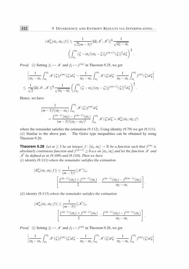
112 9 DIVERGENCE AND ENTROPY RESULTS VIA INTERPOLATING. . .
|R2m(1,2; f )| ≤ 1√
2(m−3)![( ˆK , ˆK )]
12
1√2 −1(∫ 2
1
( −1)(2 − )[ f (m+1)( )]2d) 1
2
.
Proof. (i) Setting f1 �→ K and f2 �→ f (m) in Theorem 9.25, we get∣∣∣∣ 12−1
∫ 2
1
K ( ) f (m)( )d − 12 −1
∫ 2
1
K ( )d · 12 −1
∫ 2
1
f (m)( )d∣∣∣∣
≤ 1√2[(K ,K )]
12
1√2−1
(∫ 2
1
( −1)(2 − )[ f (m+1)( )]2d) 1
2
.
Hence, we have
1(m−3)!(2−1)
∫ 2
1
K ( ) f (m)d
=f (m−1)(2)− f (m−1)(1)
(m−3)!(2−1)2
∫ 2
1
K ( )d +R1m(1,2; f )
where the remainder satisfies the estimation (9.112). Using identity (9.79) we get (9.111).(ii) Similar to the above part. The Gruss type inequalities can be obtained by usingTheorem 9.26.
Theorem 9.28 Let m ≥ 3 be an integer, f : [1,2] → R be a function such that f (m) isabsolutely continuous function and f (m+1) ≥ 0 a.e on [1,2] and let the function K and
ˆK be defined as in (9.109) and (9.110). Then we have(i) identity (9.111) where the remainder satisfies the estimation
|R1m(1,2; f )| ≤ 1
(m−3)!||K ′||[
f (m−1)(2)+ f (m−1)(1)2
− f (m−1)(2)− f 8(m−1)(1)2 −1
].
(ii) identity (9.113) where the remainder satisfies the estimation
|R1m(1,2; f )| ≤ 1
(m−3)!|| ˆK ||[
f (m−1)(2)+ f (m−1)(1)2
− f (m−1)(2)− f (m−1)(1)2 −1
].
Proof. (i) Setting f1 �→ K and f2 �→ f (m) in Theorem 9.26, we get∣∣∣∣ 12−1
∫ 2
1
K ( ) f (m)( )d − 12 −1
∫ 2
1
K ( )d · 12 −1
∫ 2
1
f (m)( )d∣∣∣∣

9.7 BOUNDS FOR THE IDENTITIES RELATED TO GENERALIZATION. . . 113
≤ 12||K ′|| 1
2 −1
∫ 2
1
( −1)(2 − )[ f (m+1)( )]2d . (9.114)
Since ∫ 21
( −1)(2 − )[ f (m+1)( )]2d =∫ 21
[2 −1−2] f m( )d
= (2 −1)[ f (m−1)(2)+ f (m−1)(1)]−2( f (m−1)(2)− f (m−1)(1)), (9.115)
using (9.79), (9.114) and (9.115), we have (9.114).(ii) Similar to above part.
Theorem 9.29 Let f : [1,2] → R be a function such that f (m−1) is absolutely con-tinuous, let x1, . . . ,xn ∈ [1,2], p1, . . . , pn ∈ (0,) be such that n
i=1 pi = 1. Also, letF21 , Gk(k = 1,2,3,4) and i(i = 1,2) are the same as defined in (9.70), (9.72)-(9.75) and
(9.1)-(9.2) respectively. Moreover, assume (p,q) such that 1 ≤ p,q,≤ , 1p + 1
q = 1 (pair
of conjugate exponent). Let | f (m)|p : [1,2] → R be Riemann integrable function. Then(i) for k = 1,3,4, we have∣∣∣∣∣i( f )−
∫ 2
1
[(m−2)
(f ′(2)− f ′(2)
2 −1
)+
12 −1
m−3
=1
(m−2−
)(
f (+1)(2)(w−2)− f (+1)(2)(w−2))]
i(Gk(·,w))dw
∣∣∣∣∣≤ 1
(2 −1)(m−3)!|| f (m)||p
(∫ 2
1
∣∣∣∣∫ 2
1
i(Gk(·,w))(w− )m−3F21 ( ,w)dw
∣∣∣∣q) 1q
,
i = 1,2. (9.116)
(ii) for k = 2, we have∣∣∣∣i( f )−∫ 2
1
[(−1)(m−2)
(f ′(2)− f ′(2)
2 −1
)+
12−1
m−3
=1
(m−2−
)( f (+1)(2)(w−2)− f (+1)(2)(w−2))
]i(G2(·,w))dw
∣∣∣∣≤ (−1)
(2 −1)(m−3)!|| f (m)||p
(∫ 2
1
∣∣∣∣∫ 2
1
i(G2(·,w))(w− )m−3F21 ( ,w)dw
∣∣∣∣q) 1q
,
i = 1,2. (9.117)
Proof. It can be proved similarly as Theorem 3.5 in [29].
Remark 9.5 We can construct the non-negative functional by taking the differences of(9.79) and (9.80). By using the idea of Section 4 and Section 5 of [28], we can constructnew class of n-exponential convexity. A new class of monotonic Cauchy means can beconstructed by using the related mean value theorem.

114 9 DIVERGENCE AND ENTROPY RESULTS VIA INTERPOLATING. . .
Remark 9.6 Following the similar way as above we can find the bounds related to thegeneralized f-divergence, Shannon and Renyi type inequalities. Further by using the gen-eralized f-divergence, Shannon and Renyi we can construct the results related to Gruss andOwstrowski type inequalities.
Remark 9.7 Analogous to the results presented in this chapter by using different inter-polating polynomials we may use inequalities (2.1), (2.27), (2.30) and (2.50) to presentrelated results.

Chapter10Integral form of Popoviciu’sInequality for ConvexFunctions
This chapter contains a new integral form of Popoviciu’s inequality. We construct newrefinement for the integral Jensen’s inequality. Also a new class of quasi-arithmetic meansalong with their monotonicity property is given. These results are published in paper (see[61]).
10.1 Integral form of Popoviciu’s Inequality
First consider some hypotheses which we use in our work given as follow.(H1) Let (X ,E ,) be a probability space, suppose p1, . . . , pn ∈ (0,) such thatn
i=1 pi = 1.(H2) Let h : X → I ⊂ R be an integrable function.(H3) Let g be a convex function on interval I, suppose such that the composition g ◦ h isintegrable.Let m ≥ 2 be a fixed integer. The -algebra in Xk generated by the projection mappingprl : Xm → X (l = 1, . . . ,m)
prl(x1, . . . ,xm) := xl (10.1)
115

116 10 INTEGRAL FORM OF POPOVICIU’S INEQUALITY FOR CONVEX FUNCTIONS
is denoted by E k. And m is defined as the product measure on E , this measure is uniquely( is -finite) specified by
m(B1× . . .×Bm) := (B1) . . .(Bk), Bl ∈ E , l = 1, . . . ,m. (10.2)
Theorem 10.1 Assume (H1)-(H3), then the following inequalities hold.
(i)
1
Cn−1m−1
1≤i1<...<im≤n
(m
j=1
pi j
) ∫Xm
g
⎛⎜⎜⎝mj=1
pi j h(xi j )
mj=1
pi j
⎞⎟⎟⎠dm(xi1 , . . . ,xim)
≤ n−mn−1
n
i=1
pi
∫X
g(h(xi))d(xi)
+m−1n−1
∫Xn
g
(n
i=1
pih(xi)
)dn(xi1 , . . . ,xin).
(ii)
1
Cn−1m−1
1≤i1<...<im≤n
(m
j=1
pi j
) ∫Xm
g
⎛⎜⎜⎝mj=1
pi j h(xi j )
mj=1
pi j
⎞⎟⎟⎠dm(xi1 , . . . ,xim)
≤n
i=1
pi
∫X
g(h(xi))d(xi).
Proof. (i) On integrating the inequality (1.24) over Xn and replacing xi j by h(xi j ), wehave
1
Cn−1m−1
1≤i1<...<im≤n
(m
j=1
pi j
)∫Xn
g
⎛⎜⎜⎝mj=1
pi j h(xi j)
mj=1
pi j
⎞⎟⎟⎠dn(xi1 , . . . ,xin)
≤ n−mn−1
n
i=1
pi
∫Xn
g(h(xi))dn(xi1 , . . . ,xin)
+m−1n−1
∫Xn
g
(n
i=1
pih(xi)
)dn(xi1 , . . . ,xin).

10.1 INTEGRAL FORM OF POPOVICIU’S INEQUALITY 117
On simplification we have
1
Cn−1m−1
1≤i1<...<im≤n
(m
j=1
pi j
) ∫Xm
g
⎛⎜⎜⎝mj=1
pi jh(xi j )
mj=1
pi j
⎞⎟⎟⎠dm(xi1 , . . . ,xim)
×∫X
d(xim+1) . . .∫X
d(xin)
≤ n−mn−1
n
i=1
pi
∫X
g ◦ h(xi)d(xi)×∫X
d(xi1) . . .∫X
d(xim)∫X
d(xim+1) . . .∫X
d(xin)
+m−1n−1
∫Xn
g
(n
i=1
pih(xi)
)dn(xi1 , . . . ,xin).
This gives
1
Cn−1m−1
1≤i1<...<im≤n
(m
j=1
pi j
) ∫Xm
g
⎛⎜⎜⎝mj=1
pi jh(xi j )
mj=1
pi j
⎞⎟⎟⎠dm(xi1 , . . . ,xim)
≤ n−mn−1
n
i=1
pi
∫X
g(h(xi))d(xi)
+m−1n−1
∫Xn
g
(n
i=1
pih(xi)
)dn(xi1 , . . . ,xin)
(ii) Applying discrete Jensen’s inequality to the last term of inequality given in (i) and onsolving, we have
1
Cn−1m−1
1≤i1<...<im≤n
(m
j=1
pi j
) ∫Xm
g
⎛⎜⎜⎝mj=1
pi jh(xi j )
mj=1
pi j
⎞⎟⎟⎠dm(xi1 , . . . ,xim)
≤ n−mn−1
n
i=1
pi
∫X
g(h(xi))d(xi)
+m−1n−1
(p1
∫Xn
g(h(x1))dn(xi1 , . . . ,xin)+ . . .+ pn
∫Xn
g(h(xn))dn(xi1 , . . . ,xin)
),
this gives

118 10 INTEGRAL FORM OF POPOVICIU’S INEQUALITY FOR CONVEX FUNCTIONS
1
Cn−1m−1
1≤i1<...<im≤n
(m
j=1
pi j
) ∫Xm
g
⎛⎜⎜⎝mj=1
pi j h(xi j)
mj=1
pi j
⎞⎟⎟⎠dm(xi1 , . . . ,xim)
≤n
i=1
pi
∫X
g(h(xi))d(xi).
10.2 New Refinement of the Integral form ofJensen’s Inequality
Under the hypothesis (H1), (H2) and (H3), define the function Hm(t) on [0,1] given by
Hm(t) =1
Cn−1m−1
1≤i1<...<im≤n
(m
j=1
pi j
)
×∫Xm
g
⎛⎜⎜⎝t
mj=1
pi j h(xi j)
mj=1
pi j
+(1− t)∫X
hd
⎞⎟⎟⎠dm(xi1 , . . . ,xim) (10.3)
Theorem 10.2 Assume (H1)-(H3), then
(i) Hm is convex.
(ii) mint∈[0,1]
Hm(t) = Hm(0) = g
(∫X
hd)
(iii) maxt∈[0,1]
Hm(t) = Hm(1)
(iv) Hm is increasing.
Proof. (i) Suppose , ∈ [0,1] with + = 1 and u,v∈ [0,1], then from (10.3) we have
Hm(u+v) =1
Cn−1m−1
1≤i1<...<im≤n
(m
j=1
pi j
)
×∫Xm
g
⎛⎜⎜⎝(u+v)
mj=1
pi j h(xi j)
mj=1
pi j
+(+ −u−v)∫X
hd
⎞⎟⎟⎠dm(xi1 , . . . ,xim).

10.2 NEW REFINEMENT OF THE INTEGRAL FORM OF JENSEN’S INEQUALITY 119
On simplification we have
Hm(u+v) =1
Cn−1m−1
1≤i1<...<im≤n
(m
j=1
pi j
)
×∫Xm
g
(
⎛⎜⎜⎝u
mj=1
pi j h(xi j )
mj=1
pi j
+(1−u)∫X
hd
⎞⎟⎟⎠+
⎛⎜⎜⎝v
mj=1
pi jh(xi j )
mj=1
pi j
+(1− v)∫X
hd
⎞⎟⎟⎠)dm(xi1 , . . . ,xim).
By convexity of g, we have
Hm(u+v)≤ 1
Cn−1m−1
1≤i1<...<im≤n
(m
j=1
pi j
)
×∫
Xm
g
⎛⎜⎜⎝u
mj=1
pi j h(xi j)
mj=1
pi j
+(1−u)∫X
gd
⎞⎟⎟⎠dm(xi1 , . . . ,xim)+
1
Cn−1m−1
1≤i1<...<im≤n
(m
j=1
pi j
) ∫Xm
g
⎛⎜⎜⎝v
mj=1
pi j h(xi j)
mj=1
pi j
+(1− v)∫X
hd
⎞⎟⎟⎠dm(xi1 , . . . ,xim),
that isHm(u+v)≤ Hm(u)+Hm(v).
Therefore Hm is convex function.(ii) Integral from of Jensen’s inequality yields
Hm(t) ≥ 1
Cn−1m−1
1≤i1<...<im≤n
(m
j=1
pi j
)
×g
⎛⎜⎜⎝∫Xm
⎛⎜⎜⎝t
mj=1
pi j h(xi j )
mj=1
pi j
+(1− t)∫X
gd
⎞⎟⎟⎠dm(xi1 , . . . ,xim)
⎞⎟⎟⎠or
Hm(t) ≥ 1
Cn−1m−1
1≤i1<...<im≤n
(m
j=1
pi j
)g(I) (10.4)

120 10 INTEGRAL FORM OF POPOVICIU’S INEQUALITY FOR CONVEX FUNCTIONS
where
I =∫
Xm
⎛⎜⎜⎝t
mj=1
pi j h(xi j)
mj=1
pi j
+(1− t)∫X
gd
⎞⎟⎟⎠dm(xi1 , . . . ,xim)
= t∫
Xm
mj=1
pi jh(xi j )
mj=1
pi j
dm(xi1 , . . . ,xim)+ (1− t)∫
Xm
⎛⎝∫X
gd
⎞⎠dm(xi1 , . . . ,xim)
=t
mj=1
pi j
m
i=1
pi
∫X
gd+(1− t)∫X
gd
=∫X
gd
so from (10.4), we have
Hm(t) ≥ 1
Cn−1m−1
1≤i1<...<im≤n
(m
j=1
pi j
)g
⎛⎝∫X
gd
⎞⎠ = Hm(0), ∀ t ∈ [0,1].
(iii)
Hm(t) = Hm(1.t +(1− t)0) ≤ tHm(1)+ (1− t)Hm(0)≤ tHm(1)+ (1− t)Hm(1)= Hm(1), ∀ t ∈ [0,1].
(iv) Since Hm(t) is convex and Hm(t)≥ Hm(0)(t ∈ [0,1]), therefore for 0 ≤ t1 < t2 ≤ 1, wehave
Hm(t2)−Hm(t1)t2− t1
≥ Hm(t2)−Hm(0)t2
≥ 0,
so
Hm(t2) ≥ Hm(t1).
Theorem 10.3 Assume (H1), (H2) and (H3), then
g
⎛⎝∫X
hd
⎞⎠ ≤ Hm(t) ≤ Hm(1) ≤∫X
g ◦ hd . (10.5)

10.3 NEW QUASI-ARITHMETIC MEANS 121
Proof. Using (ii) and (iii) of Theorem 10.2 we get first two inequalities, and for the lastinequality
Hm(1) =1
Cn−1m−1
1≤i1<...<im≤n
(m
j=1
pi j
)×
∫Xm
g
⎛⎜⎜⎝mj=1
pi jh(xi j )
mj=1
pi j
⎞⎟⎟⎠dm(xi1 , . . . ,xim).
Using discrete Jensen’s inequality, we have
Hm(1) ≤ 1
Cn−1m−1
1≤i1<...<im≤n
(m
j=1
pi j
)×
mj=1
pi j
mj=1
pi j
∫Xm
g(h(xi j)
)dm(xi1 , . . . ,xim),
this gives
Hm(1) ≤∫X
g ◦ hd .
Remark 10.1 A refinement similar to (10.5) of integral form of Jensen’s inequality isproved in Proposition 7 of [49].
10.3 New Quasi-Arithmetic Means
Now we introduce some new quasi arithmetic means. First we assume the following con-ditions:(H4) Let h : X → I, where I ⊂ R be an interval, is measurable.(H5) Let and be two real valued, continuous and strictly monotone functions definedon interval I.
Definition 10.1 Assume (H1), (H4) and (H5).For t ∈ [0,1] we define the class of quasi-arithmetic means given by
M ,(t,g,) := −1(
1
Cn−1m−1
1≤i1<...<im≤n
(m
j=1
pi j
)
×∫
Xm
◦−1
⎛⎜⎜⎝t
mj=1
pi j (g(xi j ))
mj=1
pi j
+(1− t)∫X
(g)d
⎞⎟⎟⎠dm(xi1 , . . . ,xim))
(10.6)
where the integrals are supposed to exist.

122 10 INTEGRAL FORM OF POPOVICIU’S INEQUALITY FOR CONVEX FUNCTIONS
Assume (H6), let be a real valued, continuous and strictly monotone function definedon interval I such that the composition ◦ h is integrable on X , and M(h,) is the quasi-arithmetic mean defined in (2.16).
Theorem 10.4 Assume (H1),(H4), (H5) and assume that ◦ h and ◦ h are integrableon X.(i) If ◦−1 is convex with is increasing or ◦−1 is concave with is decreasing,then
M (h,) ≤ M , (t,h,) ≤ M(h,), (10.7)
holds for all t ∈ [0,1].(ii) If ◦−1 is convex with is decreasing or ◦−1 is concave with is increasing,then
M (h,) ≥ M , (t,h,) ≥ M(h,), (10.8)
holds for all t ∈ [0,1].
Proof. (i) Using pair of functions ◦−1 and (h) ( (I) is an interval) in Theorem 10.3,we have
◦−1
⎛⎝∫X
(h)d
⎞⎠ ≤ 1
Cn−1m−1
1≤i1<...<im≤n
(m
j=1
pi j
)
×∫Xm
◦−1
⎛⎜⎜⎝t
mj=1
pi j (h(xi j ))
mj=1
pi j
+(1− t)∫X
(h)d
⎞⎟⎟⎠dm(xi1 , . . . ,xim)
≤ 1
Cn−1m−1
1≤i1<...<im≤n
(m
j=1
pi j
) ∫Xm
◦−1
⎛⎜⎜⎝mj=1
pi j (h)
mj=1
pi j
⎞⎟⎟⎠dm(xi1 , . . . ,xim)
Using the discrete Jensen inequality on the larger side of last inequality we get
◦−1
⎛⎝∫X
(h)d
⎞⎠ ≤ 1
Cn−1m−1
1≤i1<...<im≤n
(m
j=1
pi j
)
×∫Xm
◦−1
⎛⎜⎜⎝t
mj=1
pi j (h(xi j ))
mj=1
pi j
+(1− t)∫X
(h)d
⎞⎟⎟⎠dm(xi1 , . . . ,xim)
≤∫X
(h)d
On taking −1 on both sides we have (10.7).(ii) Similarly using the pair of functions − ◦ −1 and (h) in Theorem 1.14, where ◦−1 is concave. On taking −1 we have (10.8).

Chapter11Refinement of Jensen’sInequality for 3-convexFunctions
We use (1.14) and establish the inequalities for classes of functions K a1 (I) and K a
2 (I), asit was done for convex functions. We also improve these inequalities. These results can befound in [62].
11.1 Refinement of Jensen’s Inequality for 3-convexFunctions at a Point
In [25], I. A. Baloch et al. introduced the new classes of functions that are K a1 (I) and
K a2 (I) given in the following definition.
Definition 11.1 Let f : I → R and a ∈ I◦ (I◦ denotes the interior of I). Consider theclasses
K a1 (I) :=
{f : there exists a real number B such that f (x)− B
2x2is concave on
I∩ (−,a]and convex onI∩ [a,)}(11.1)
123

124 11 REFINEMENT OF JENSEN’S INEQUALITY FOR 3-CONVEX FUNCTIONS
and
K a2 (I) :=
{f : there exists a real number B such that f (x)− B
2x2is convex on
I∩ (−,a]and concave onI∩ [a,)} .
(11.2)
The function f ∈ K a1 (I) is called 3-convex function at the point a. The function f ∈
K a2 (I)) is called 3-concave function at the point a.
They also showed that the K a1 (I)(K a
2 (I)) is larger class of functions than the class of all3-convex (3-concave) functions in the following result (see [25], Theorem 2.4).
Theorem 11.1 If g∈K a1 (I)(g ∈K a
2 (I)) for every a∈ I, then g is 3-convex (3-concave).
In [25], I. A. Baloch et al. gave the Levinson inequality for the classes K a1 (I) and
K a2 (I).
Theorem 11.2 Let I = [, ] be an interval. Consider x = (x1, . . . ,xn) ∈ [, ]n andy = (y1, . . . ,ys) ∈ [, ]s. Also let there exist a ∈ I such that
maxi
xi ≤ a ≤ minj
y j.
Suppose p = (p1, . . . , pn) ∈ (0,)n, q = (q1, . . . ,qs)s ∈ (0,)s such thatnj=1
p j =si=1
qi = 1
and
Am,r(Im,x,p, id2)−Am,k(Im,x,p, id2) =
Am,r(Im,y,q, id2)−Am,k(Im,y,q, id2). (11.3)
If f ∈ K a1 (I), then
Am,r(Im,x,p, f )−Am,k(x,p, f ) ≤ Am,r(y,q, f )−Am,k(y,q, f ) (11.4)
holds for Am,r defined in (1.13).
Proof. Since H1(x) := f (x)− B2 x2 is concave on I∩ [,a], therefore from Remark 9.3, we
have
0 ≥ Am,r(x,p,H1)−Am,k(x,p,H1)
= Am,r(x,p, f )−Am,k(x,p, f )− B2
[Am,r(x,p, id2)
− Am,k(x,p, id2)]. (11.5)
As H2(y) := f (y)− B2 y2 is convex on [a, ], therefore from Remark 9.3, we get
0 ≤ Am,r(y,p,H2)−Am,k(y,p,H2)

11.1 REFINEMENT OF JENSEN’S INEQUALITY FOR 3-CONVEX FUNCTIONS. . . 125
= Am,r(y,p, f )−Am,k(y,p, f )− B2
[Am,r(y,p, id2)
− Am,k(y,p, id2)]. (11.6)
From (11.5) and (11.6), we have
Am,r(x,p, f )−Am,k(x,p, f )− B2
[Am,r(x,p, id2)−Am,k(x,p, id2)
]≤ Am,r(y,p, f )−Am,k(y,p, f )− B
2
[Am,r(y,p, id2)−Am,k(y,p, id2)
].
Using the assumption (11.3), we get (11.4).
Corollary 11.1 Let I = [0,2a] be an interval, x = (x1, . . . ,xn) ∈ [0,a]n, y = (y1, . . . ,ym) ∈[a,2a]m and p = (p1, . . . , pn) be positive n-tuple such that
nj=1
p j = 1, also let
x1 + y1 = . . . = xn + yn = 2a.
If f ∈ K a1 (I), then the inequality (11.4) holds for n = m and p = q.
Proof. Note that
id2
⎛⎜⎜⎜⎝kj=1
pi j yi j
kj=1
pi j
⎞⎟⎟⎟⎠ = id2
⎛⎜⎜⎜⎝kj=1
pi j (c− xi j)
kj=1
pi j
⎞⎟⎟⎟⎠ (11.7)
= c2−2c
kj=1
pi j xi j
kj=1
pi j
+
⎛⎜⎜⎜⎝kj=1
pi j xi j
kj=1
pi j
⎞⎟⎟⎟⎠2
. (11.8)
We can observe that
Am,r(x,p, id2)−Am,k(x,p, id2) = Am,r(y,p, id2)−Am,k(y,p, id2).
Following the same steps as in Theorem 11.2, we get (11.4).
Remark 11.1 Using (11.5) and (11.6) from proof of Theorem 11.2, we have
Am,r(x,p, f ) − Am,k(x,p, f ) ≤ B2
[Am,r(x,p, id2) − Am,k(x,p, id2)
](11.9)
and

126 11 REFINEMENT OF JENSEN’S INEQUALITY FOR 3-CONVEX FUNCTIONS
B2
[Am,r(y,p, id2) − Am,k(y,p, id2)
]≤ Am,r(y,p, f ) − Am,k(y,p, f ). (11.10)
Using (11.9) and (11.10), we have the refinement of (11.4) given by
Am,r(x,p, f )−Am,k(x,p, f ) ≤ B2
[Am,r(x,p, id2)−Am,k(x,p, id2)
](
=B2
[Am,r(y,p, id2)−Am,k(y,p, id2)
])≤ Am,r(y,p, f )−Am,k(y,p, f ).
The next result is the generalization of Theorem 11.2, with weaker assumptions on (11.3).
Theorem 11.3 Let I = [, ] be an interval, x = (x1, . . . ,xn) ∈ [, ]n, y = (y1, . . . ,ys) ∈[, ]s with
maxi
xi ≤ minj
y j. (11.11)
Also let p = (p1, . . . , pn) ∈ (0,)n, q = (q1, . . . ,qs) ∈ (0,)s such thatnj=1
p j =si=1
qi = 1
and f ∈ K a1 (I) for some a ∈ [maxxi,miny j]. Then if
(i)f ′′−(maxxi) ≥ 0
andAm,r(x,p, id2)−Am,k(x,p, id2) ≤ Am,r(y,q, id2)−Am,k(y,q, id2)
(ii)f ′′+(miny j) ≤ 0
andAm,r(x,p, id2)−Am,k(x,p, id2) ≥ Am,r(y,q, id2)−Am,k(y,q, id2)
(iii) f ′′−(maxxi) < 0 < f ′′+(miny j) and f is 3-convex,
then (11.4) holds.
Proof. Since f ∈ K a1 [, ] for some a ∈ [maxxi,maxy j], therefore there exists a constant
B such that H1(x) := f (x)− B2 x2, is concave on [,a], such that for x1, . . . ,xn ∈ I∩ [,a],
we have
0 ≥ Am,r(x,p,H1)−Am,k(x,p,H1),
that is
0 ≥ Am,r(x,p, f )−Am,k(x,p, f )− B2
[Am,r(x,p, id2)
− Am,k(x,p, id2)]. (11.12)

11.1 REFINEMENT OF JENSEN’S INEQUALITY FOR 3-CONVEX FUNCTIONS. . . 127
Also H2(y) := f (y)− B2 y2 is convex on [a, ], for y1, . . . ,ys ∈ [a, ], we have
0 ≤ Am,r(y,p,H2)−Am,k(y,p,H2),
that is
0 ≥ Am,r(y,p, f )−Am,k(y,p, f )− B2
[Am,r(y,p, id2)
− Am,k(y,p, id2)]. (11.13)
From (11.12) and (11.13), we have
Am,r(x,p, f )−Am,k(x,p, f )− B2
[Am,r(x,p, id2)−Am,k(x,p, id2)
]≤ Am,r(y,p, f )−Am,k(y,p, f )− B
2
[Am,r(y,p, id2)−Am,k(y,p, id2)
].
So
B2
[Am,r(y,p, id2)−Am,k(y,p, id2)−Am,r(x,p, id2)−Am,k(x,p, id2)
]≤ Am,r(y,p, f )−Am,k(y,p, f )−Am,r(x,p, f )−Am,k(x,p, f ). (11.14)
Now due to concavity of H1 and convexity of H2 for every distinct point x j ∈ [,maxxi]and y j ∈ [minyi, ], j = 1,2,3, we have
[x1, x2, x3, f ] ≤ B ≤ [y1, y2, y3, f ]. (11.15)
Letting x j ↗ maxxi and y j ↘ miny j, we get the inequalities if derivatives exist
f ′′−(maxxi) ≤ B ≤ f ′′+(minyi). (11.16)
Since from assumption (a), f ′′(maxxi) ≥ 0, therefore B ≥ 0, so using the assumption[Am,r(y,p, id2)−Am,k(y,p, id2)−Am,r(x,p, id2)−Am,k(x,p, id2)
] ≥ 0,
the expression
B2
[Am,r(y,p, id2)−Am,k(y,p, id2)−Am,r(x,p, id2)−Am,k(x,p, id2)
]is non-negative and on using it on left side of (11.14) we have the result (11.4). And simi-larly for assumption (b), the inequality f ′′+(miny j) ≤ 0 gives B ≤ 0, so the expression withassumption of (b) is also non-negative, this gives the result (11.4). Under the assumptionof (c), f ′′− and f ′′+ are both left and right continuous respectively and both are nondecreas-ing with f ′′− ≤ f ′′+, so their exists a point a ∈ [maxxi,miny j] such that f ∈ K a
1 [, ] withconstant B = 0, and thus we have the inequality (11.4).

128 11 REFINEMENT OF JENSEN’S INEQUALITY FOR 3-CONVEX FUNCTIONS
Remark 11.2 From the proof of Theorem 11.3, we have
Am,r(x,p, f )−Am,k(x,p, f ) ≤ B2
[Am,r(x,p, id2)−Am,k(x,p, id2)
]and
Am,r(y,p, f )−Am,k(y,p, f ) ≥ B2
[Am,r(y,p, id2)−Am,k(y,p, id2)
].
In Theorem 11.3, B is positive, negative and zero for the assumptions (a), (b) and (c)respectively as discussed in proof. Therefore, we have the better improvement of (11.4)than (11.11) given as
Am,r(x,p, f )−Am,k(x,p, f ) ≤ B2
[Am,r(x,p, id2)−Am,k(x,p, id2)
]≤ B
2
[Am,r(y,p, id2)−Am,k(y,p, id2)
] ≤ Am,r(y,p, f )−Am,k(y,p, f ).
If the assumptions of Theorem 11.2 with f ∈ K a2 [, ], the reverse of inequality (11.4)
holds. The generalization of this result is proven in the following result.
Theorem 11.4 Let I = [, ]⊂R be an interval, x= (x1, . . . ,xn)∈ [, ]n, y = (y1, . . . ,ys)∈[, ]s with
maxi
xi ≤ minj
y j. (11.17)
Also let p = (p1, . . . , pn) ∈ (0,)n, q = (q1, . . . ,qs) ∈ (0,)s such thatnj=1
p j = 1 =si=1
qi
and f ∈ K a2 (I) for some a ∈ [maxxi,miny j]. Then if
(i)f ′′−(maxxi) ≤ 0
andAm,r(x,p, id2)−Am,k(x,p, id2) ≤ Am,r(y,q, id2)−Am,k(y,q, id2)
(ii)f ′′+(miny j) ≥ 0
andAm,r(x,p, id2)−Am,k(x,p, id2) ≥ Am,r(y,q, id2)−Am,k(y,q, id2)
(iii) f ′′−(maxxi) < 0 < f ′′+(miny j) and f is 3-concave,
then the inequality
Am,r(x,p, f )−Am,k(x,p, f ) ≥ Am,r(y,q, f )−Am,k(y,q, f ) (11.18)
holds.

11.1 REFINEMENT OF JENSEN’S INEQUALITY FOR 3-CONVEX FUNCTIONS. . . 129
Proof. Since f ∈ K a2 [, ] for some a ∈ [maxxi,maxy j], therefore there exists a constant
B such that H1(x) = f (x)− B2 x2, is convex on I ∩ (−,a], such that for x1, . . . ,xn ∈ I ∩
(−,a], we have
0 ≤ Am,r(x,p,H1)−Am,k(x,p,H1),
that is
0 ≤ Am,r(x,p, f )−Am,k(x,p, f )− C2
[Am,r(x,p, id2)
− Am,k(x,p, id2)]. (11.19)
Also H2(y) = f (y)− B2 y2 is concave on I∩ [a,), for y1, . . . ,ys ∈ [a,), we have
0 ≥ Am,r(y,p,H2)−Am,k(y,p,H2),
that is
0 ≥ Am,r(y,p, f )−Am,k(y,p, f )− B2
[Am,r(y,p, id2)
− Am,k(y,p, id2)]. (11.20)
From (11.19) and (11.20), we have
Am,r(x,p, f )−Am,k(x,p, f )− B2
[Am,r(x,p, id2)−Am,k(x,p, id2)
]≥ Am,r(y,p, f )−Am,k(y,p, f )− B
2
[Am,r(y,p, id2)−Am,k(y,p, id2)
].
So
B2
[Am,r(y,p, id2)−Am,k(y,p, id2)−Am,r(x,p, id2)−Am,k(x,p, id2)
]≥ Am,r(y,p, f )−Am,k(y,p, f )−Am,r(x,p, f )−Am,k(x,p, f ). (11.21)
Now due to convexity of H1 and concavity of H2 for every distinct point x j ∈ [,maxxi]and y j ∈ [minyi, ], j = 1,2,3, we have
[x1, x2, x3, f ] ≥ B ≥ [y1, y2, y3, f ]. (11.22)
Letting x j ↗ maxxi and y j ↘ miny j, we get the inequalities if derivatives exist
f ′′−(maxxi) ≥ B ≥ f ′′+(minyi). (11.23)
Since from assumption (a), f ′′(maxxi) ≤ 0, therefore B ≥ 0, using the assumption[Am,r(y,p, id2)−Am,k(y,p, id2)−Am,r(x,p, id2)−Am,k(x,p, id2)
] ≥ 0

130 11 REFINEMENT OF JENSEN’S INEQUALITY FOR 3-CONVEX FUNCTIONS
we have
B2
[Am,r(y,p, id2)−Am,k(y,p, id2)−Am,r(x,p, id2)−Am,k(x,p, id2)
]is negative and on using it on left side of (11.21) we have the result (11.4). And similarlyfor assumption (b), the inequality f ′′+(miny j) ≥ 0 gives B > 0, so the expression withassumption of (b) is also positive, this gives the result (11.4). Under the assumption of (c),f ′′− and f ′′+ are left and right continuous respectively and both are decreasing with f ′′− ≥ f ′′+,so there exists a point a∈ [maxxi,miny j] such that f ∈K a
1 [, ] with constant B = 0, andthus we have the inequality (11.18).
Remark 11.3 In Theorem 11.4, B is negative or positive or zero under the assumption(i),(ii) and (iii) respectively as discussed earlier in the proof of the Theorem 11.4. There-fore we get the improvement of (11.18) as follows.
Am,r(x,p, f )−Am,k(x,p, f ) ≥ Am,r(x,p, id2)−Am,k(x,p, id2)
≥ Am,r(y,q, id2)−Am,k(y,q, id2) ≥ Am,r(y,q, f )−Am,k(y,q, f ).
Remark 11.4 Theorem 11.2, Remark 11.1, Theorem 11.3, Remark 11.2 and Theorem11.4 are also valid for the differences given in (9.1) and (9.2) for r = 1, . . . ,m and 1 ≤ r <k ≤ m respectively.
Bibliography
[1] S. Abramovich, M. Klaricic Bakula, M. Matic and J. Pecaric, A variant of Jensen-Steffensen’s inequality and quasi-arithmetic means, J. Math. Anal. Appl., 307(2005), 370–386.
[2] M. Adil Khan, D. Pecaric, J. Pecaric, New refinement of the Jensen inequality as-sociated to certain functions with applications, J. Inequal. Appl., (2020) Article ID76, 11 pages.
[3] M. Adil Khan, D. Pecaric, J. Pecaric, A new refinement of the Jensen inequality withapplications in information theory, Bull. Malays. Math. Sci. Soc., (accepted).
[4] M. Adil Khan, D. Pecaric, J. Pecaric, Refined Jensen-Steffensen’s inequality, sub-mitted.
[5] M. Adil Khan, J. Pecaric, New refinements of the Jensen-Mercer inequality associ-ated to positive n-tuples, submitted.
[6] M. Adil Khan, J. Pecaric, Refinement of the Jensen inequality for convex functionsof several variables with applications, submitted.
[7] M. Adil Khan, J. Pecaric, Y.-M. Chu, Refinements of Jessen’s and McShane’s in-equalities with applications, submitted.
[8] M. Adil Khan, J. Pecaric, A refinement of the Jensen operator inequality associatedto n-tuple with applications, submitted.
[9] M. Adil Khan, Z. M. Al-sahwi and Y.-M. Chu, New estimations for Shannon andZipf-Mandelbrot entropies, Entropy., 20(608) (2018), 1–10.
[10] M. Adil Khan, M. Hanif, Z. A, Khan, K. Ahmad and Y.-M. Chu, Association ofJensen inequality for s-convex function, J. Inequal. Appl., 2019, Article ID 162, 14pages.
[11] M. Adil Khan, J. Khan, and J. Pecaric, Generalization of Jensen’s and Jensen-Steffensen’s inequalities by generalized majorization theorem, J. Math. Inequal.,11(4) (2017), 1049–1074.
[12] M. Adil Khan, D. Pecaric, J. Pecaric, On Zipf-Mandelbrot entropy, J. Comput. Appl.Math., 346 (2019), 192–204.
[13] M. Adil Khan, D. Pecaric and J. Pecaric, Bounds for Shannon and Zipf-Mandelbrotentropies, Math. Methods Appl. Sci., 40(18) (2017), 7316–7322.
131

132 11 BIBLIOGRAPHY
[14] M. Adil Khan, S. Zaheer Ullah and Y.-M. Chu, The concept of coordinate stronglyconvex functions and related inequalities, Rev. R. Acad. Cienc. Exactas Fıs. Nat.Ser. A Mat. RACSAM., 113 (2019), 2235–2251.
[15] R. P. Agarwal and P. J. Y. Wong, Error inequalities in polynomial interpolation andtheir applications, Kluwer Academic Publishers, Dordrecht/Boston/London (1993).
[16] A. A. Aljinovic, J. Pecaric and A. Vukelic, On some Ostrowski type inequalitiesvia Montgomery identity and Taylor’s formula II, Tamkang J. Math., 36(4) (2005),279–301.
[17] A. A. Aljinovic and J. Pecaric, On some Ostrowski type inequalities via Montgomeryidentity and Taylor’s formula, Tamkang J. Math., 36(3) (2005), 199–218.
[18] G. Anderson and Y. Ge, The size distribution of Chinese cities, Regional Scienceand Urban Economics, 35(6) (2005), 756–776.
[19] F. Auerbach, Das Gesetz der Bevolkerungskonzentration, Petermanns Geographis-che Mitteilungen, 59 (1913), 74–76.
[20] M. K. Bakula and K. Nikodem, Converse Jensen inequality for strongly convexset-valued maps, J. Math. Inequal., 12(2) (2018), 545–550.
[21] E. Beck, Uber Ungleichungen von der Form f (M (x;);M (y;)) ≥M( f (x;y);), Univ. Beograd. Publ. Elektrotehn. Fak. Ser. Mat. Fiz., 320–328(1970), 1–14.
[22] P. Beesack, On the Green’s function of an N-point boundary value problem, PacificJ. Math., 12(3) (1962), 801–812.
[23] D. Black and V. Henderson, Urban evolution in the USA, J. Econ. Geography., 3(4)(2003), 343–372.
[24] M. Bosker, S. Brakman, H. Garretsen and M. Schramm, A century of shocks: theevolution of the German city size distribution, 1925–1999, Regional Science andUrban Economics, 38(4) (2008), 330–347.
[25] I. Brnetic, C. E. M. Pearce and J. Pecaric, Refinements of Jensen’s inequality,Tamkang J. Math., 31 (2000), 63–69.
[26] P. S. Bullen, Handbook of means and their inequalities, KluwerAcademicPublisher,(2003), pp. 537.
[27] P. S. Bullen, D. S. Mitrinovic and P. M. Vasic, Means and their inequalities, KluwerAcademic Publisher, (1988).
[28] S. I. Butt, K. A. Khan and J. Pecaric, Popoviciu Type Inequalities via Green Func-tion and Generalized Montgomery Identity, Math. Inequal. Appl., 18(4) (2015),1519–1538.
[29] S. I. Butt, K. A. Khan and J. Pecaric, Generalization of Popoviciu inequality forhigher order convex function via Taylor’s polynomial, Acta Univ. Apulensis Math.Inform, 42 (2015), 181–200.
[30] S. I. Butt, K. A. Khan and J. Pecaric, Popoviciu type inequalities via Hermite’spolynomial, Math. Inequal. Appl., 19(4) (2016), 1309–1318.

11.1 BIBLIOGRAPHY 133
[31] S. I. Butt, N. Mehmood and J. Pecaric, New generalizations of Popoviciu type in-equalities via new green functions and Fink’s identity, Transactions of A. RazmadzeMathematical Institute, 171(3) (2017), 293–303.
[32] S. I. Butt and J. Pecaric, Popoviciu’s Inequality For N-convex Functions, Lap Lam-bert Academic Publishing, (2016).
[33] S. I. Butt and J. Pecaric, Weighted Popoviciu type inequalities via generalized Mont-gomery identities, Rad Hrvat. Akad. Znan. Umjet. Mat. Znan., 19 (2015), 69–89.
[34] P. Cerone and S. S. Dragomir, Some new Ostrowski-type bounds for the Cebysevfunctional and applications, J. Math. Inequal., 8(1) (2014), 159–170.
[35] D. Choi, M. Krnic and J. Pecaric, More accurate classes of Jensen-type inequali-ties for convex and operator convex functions, Math. Inequal. Appl., 21(2) (2018),301–321.
[36] I. Csiszar, Information measures: a critical survey, In: Tans. 7th Prague Conf. onInfo. Th., Statist. Decis. Funct., Random Process and 8th European Meeting ofStatist., Academia Prague., B (1978), 73–86.
[37] I. Csiszar, Information-type measures of difference of probability distributions andindirect observations, Stud. Sci. Math. Hungar., 2 (1967), 299–318.
[38] V. Culjak, B. Ivankovic and J. Pecaric, On Jensen–Mcshane’s inequality, Period.Math. Hungar., 58(2) (2009), 139–154.
[39] A. P. Dempster, N. M. Laird and D. B. Rubin, Maximum Likelihood from IncompleteData via the EM Algorithm, J. R. Stat. Soc. Ser. B Stat. Methodol., (1977), 1–38.
[40] S. S. Dragomir and C. E. M. Pearce, Selected topics on Hermite-Hadamard inequal-ities and applications, Victoria University, 2000.
[41] A. M. Fink, Bounds on the deviation of a function from its averages, CzechoslovakMath. J., 42(2) (1992), 289–310.
[42] T. Furuta, J. M. Hot, J. Pecaric and Y. Seo, Mond-Pecaric Method in OperatorInequalities, Element, Zagreb, (2005).
[43] T. Furuta and J. Pecaric, An operator inequality associated with the operator con-cavity of operator entropy a loga−1, Math. Inequal. Appl., 6(3) (2003), 531–543.
[44] A. L. Gibbs, On Choosing and boundary probability metrics, Int. Stat. Rev. 70(2002), 419–435.
[45] L. Horvath, K. A. Khan and J. Pecaric, Cyclic refinements of the discrete and integralform of Jensen’s inequality with applications, Analysis., 36(4) (2016), 253–262.
[46] L. Horvath, K. A. Khan and J. Pecaric, Refinements of Holder and Minkowskiinequalities with weights, Proc. A. Razmadze Math. Inst., 158 (2012), 33–56.
[47] L. Horvath, K. A. Khan and J. Pecaric, Combinatorial improvements of Jensen’sinequality / Classical and new refinements of Jensen’s inequality with applications,Monographs in inequalities 8, Element, Zagreb, (2014), pp. 229.
[48] L.Horvath, K.A.Khan and J. Pecaric,Refinement of Jensen’s inequality for operatorconvex functions, Adv. Inequal. Appl., 2014 (2014), 1–17.
134 11 BIBLIOGRAPHY
[49] L. Horvath and J. Pecaric, Refinement of the classical Jensen’s inequality comingfrom refinement of the discrete Jensen’s inequality, Adv. Inequal. Appl., 2015, Arti-cle ID 8, 323–328.
[50] L. Horvath and J. Pecaric, A refinement of discrete Jensen’s inequality, Math. In-equal. Appl., 14 (2011), 777–791.
[51] L. Horvath, D. Pecaric and J. Pecaric, Estimations of f and Renyi divergences byusing a cyclic refinement of the Jensen’s inequality, Bull. Malays. Math. Sci. Soc.,42 (2019), 933–946.
[52] L. Horvath, D. Pecaric and J. Pecaric, Estimations of f -and Renyi divergences byusing a cyclic refinement of the Jensen’s inequality, Bull. Malays. Math. Sci. Soc.,(2017), 1–14.
[53] J. M. Hot, J. Pecaric and Y. Seo, Order among quasi-arithmetic means of positiveoperators, Math. Rep., 14(64) (2012), 71–86.
[54] J. M. Hot and Y. Seo, An interpolation of Jensen’s inequality and its converses withapplications to quasi-arithmetic mean inequalities, J. Math. Inequal., 12(2) (2018),303–313.
[55] Y. M. Ioannides and H. G. Overman, Zipf’s law for cities: an empirical examination,Regional science and urban economics, 33(2) (2003), 127–137.
[56] I. Iscan, New refinements for integral and sum forms of Holder inequality, J. Inequal.Appl., 2019, Article ID 304, 11 pages.
[57] B. Jessen, Bemrkninger om konvekse Funktioner og Uligheder imellem Mid-delvrdier, I, Matematisk Tidsskrift B, 2 (1931), 17–28.
[58] J. Khan, M. Adil Khan and J. Pecaric, On Jensen’s type inequalities via generalizedmajorization Inequalities, Filomat., 32(16) (2018), 5719–5733.
[59] K. A. Khan, T. Niaz, D. Pecaric and J. Pecaric, Estimation of different entropies viaLidstone polynomial using Jensen type functionals, Arabian J. Math., (2018), 1–19.
[60] K. A. Khan, T. Niaz, D. Pecaric and J. Pecaric, Refinement of Jensen’s inequalityand estimation of f-and Renyi divergence via Montgomery identity, J. Inequal.Appl.,2018(1) (2018), 22 pages.
[61] K. A. Khan, T. Niaz and J. Pecaric, Integral Form of Popoviciu Inequality for ConvexFunction, Proceeding of Pakistan academy of sciences: A. Phys. Comput. Sci., 53(3)(2016), 339–348.
[62] K. A. Khan, T. Niaz and J. Pecaric, On Refinement of Jensen’s type Inequality for3-convex function, Turkish Journal of Inequalities, 4(1), (2020).
[63] K. A. Khan, T. Niaz, D. Pecaric, and J. Pecaric, Estimation of different entropies viaAbel Gontscharoff Green functions and Fink’s identity using Jensen type functionals,Arab J. Math. Sci., (2018), DOI 10.1016/j.ajmsc.2018.12.002.
[64] K. A. Khan, T. Niaz, D. Pecaric and J. Pecaric, Estimation of different entropiesvia Hermite interpolating polynomial using Jensen type functionals, The journal ofAnalysis (accepted).

11.1 BIBLIOGRAPHY 135
[65] S. Kullback, Information theory and statistics, Courier Corporation., (1997).
[66] S. Kullback and R. A. Leibler, On information and sufficiency, The annals of math-ematical statistics, 22(1) (1951), 79–86.
[67] N. Latif, D. Pecaric and J. Pecaric, Majorization, useful Csiszar divergence anduseful Zipf-Mandelbrot law, Open Math., 16 (2018), 1357–1373.
[68] A. Y. Levin, Some problems bearing on the oscillation of solution of liear differentialequations, Soviet Math. Dokl., 4 (1963), 121–124.
[69] F. Leise and I. Vajda, Convex Statistical Distance (Teubner-Text Zur Mathemmatik),Teubner, Leipzig, 95 (1987).
[70] N. Lovricevic, D, Pecaric and J. Pecaric, Zipf-Mandelbrot law, f-divergences andthe Jensen-type interpolating inequalities, J. Inequal. Appl., 36(1) (2018), 20 pages.
[71] G. Lu, New refinements of Jensen’s inequality and entropy upper bounds, J. Math.Inequal., 12(2) (2018), 403–421.
[72] D. Y. Manin, Mandelbrot’s Model for Zipf’s Law: Can Mandelbrot’s Model explainZipf’s law for language, J. Quant. Linguist., 16(3) (2009), 274–285.
[73] B. Mandelbrot, Information Theory and Psycholinguistics: A Theory of Words Fre-quencies, In Reading in Mathematical Social Scence. (ed.) P. Lazafeld, N. Henry.Cambridge MA, MIT Press, (1966).
[74] M. Matic, C. E. Pearce and J. Pecaric, Shannon’s and related inequalities in in-formation theory, In Survey on Classical Inequalities. Springer, Dordrecht, (2000),127–164.
[75] D. S. Mitrinovic, J. Pecaric and A. M. Fink, Classical and New Inequalities inAnalysis, Kluwer Academic Publisher, (1993).
[76] R. Mikic, D. Pecaric and J. Pecaric, Inequalities of the Jensen and Edmundson-Lah-Ribaric type for 3-convex functions with applications, J. Math. Inequal., 12(3)(2018), 677–692.
[77] A. McD. Mercer, A variant of Jensen’s inequality, JIPAM 4 (2003), Article 73.
[78] E. J. McShane, Jensen’s inequality, Bull. Amer. Math. Soc., 43(8) (1937), 521–527.
[79] M. A. Montemurro, Beyond the Zipf-Mandelbrot law in quantitative linguistics,(2001) URL: arXiv:cond-mat/0104066v2 (22.2.2017.)
[80] D. Mouillot and A. Lepretre, Introduction of relative abundance distribution (RAD)indices, estimated from the rank-frequency diagrams (RFD), to assess changes incommunity diversity, Environ. Monitoring Assess., 63(2), (2000), 279–295.
[81] H. R. Moradi, M. E. Omidvar, M. Adil Khan and K. Nikodem, Around Jensen’sinequality for strongly convex functions, Aequationes Math., 92(1) (2018), 25–37.
[82] T. Niaz, K. A. Khan, D. Pecaric and J. Pecaric, Estimation of different entropies viaTaylor one point and Taylor two points interpolations using Jensen type functionals,Int. J. Anal. Appl., 17(5) (2019), 686–710.

136 11 BIBLIOGRAPHY
[83] T. Niaz, K. A. Khan and J. Pecaric, On generalization of refinement of Jensen’sinequality using Fink’s identity and Abel-Gontscharoff Green function, J. Inequal.Appl., 2017(1) (2017), 12 pages.
[84] J. Pecaric, Remark on an inequality of S. Gabler, J. Math. Anal. Appl., 184(1)(1994), 19-21.
[85] J. Pecaric, K. A. Khan and I. Peric, Generalization of Popoviciu type inequalities forsymmetric means generated by convex functions, J. Math. Comput. Sci., 4(6) (2014),1091.
[86] J. Pecaric and J. Peric, New improvement of the converse Jensen inequality, Math.Inequal. Appl., 21(1) (2018), 217–234.
[87] J. Pecaric, F. Proschan, Y. L. Tong, Convex Functions, Partial Orderings and Statis-tical Applications, Academic Press, New York, (1992).
[88] J. Pecaric and V. Volenec, Interpolation of the Jensen inequality with some appli-cations, Osterreich. Akad. Wiss. Math.-Natur. Kl Sonderdruck Sitzungsber, 197(1988), 463–476.
[89] A. Renyi, On measure of information and entropy, In: Proceeding of the FourthBerkely Symposium on Mathematics, Statistics and Probability, (1960), 547–561.
[90] K. T. Rosen and M. Resnick, The size distribution of cities: an examination of thePareto law and primacy, J. Urban Econ., 8(2) (1980), 165–186.
[91] M. Sababheh, Improved Jensen’s inequality, Math. Inequal. Appl., 20(2) (2017),389–403.
[92] I. Sason, S. Verdu, f -divergence inequalities, IEEE Trans. Inf. Theory., 62 (2016),5973–6006.
[93] C. E. Shannon, A mathematical theory of communication, Bell Syst. Tech. J., 27(1948), 379–423, 623–656.
[94] Z. K. Silagadze, Citations and the Zipf-Mandelbrot Law, Complex Syst., 11 (1997),487–499.
[95] K. T. Soo, Zipf’s Law for cities: a cross-country investigation, Regional science andurban Economics, 35(3) (2005), 239-263.
[96] J. F. Steffensen, On certain inequalities and methods of approximation, J. Inst.Actuaries., 51 (1919), 274–297.
[97] Y.-Q. Song, M. Adil Khan, S. Zaheer Ullah and Y.-M. Chu, Integral inequalities forstrongly convex functions, J. Funct. Spaces., 2018, Article ID 6595921, 8 pages.
[98] I. Vajda, Theory of Statistical Inference and Information, Kluwer, Dordrecht, (1989).
[99] D. V. Widder, Completely convex function and Lidstone series, Trans. Am. Math.Soc. 51 (1942), 387–398.
[100] G. K. Zipf, Human behaviour and the principle of least-effort, Cambridge MA edn.Reading: Addison-Wesley, (1949).

Index
Abel-Gontscharoff polynomial, 103Lagrange polynomial, 94
Bhattacharyya coefficient, 27
Cebysev functional, 110Convex function
— in Jensen sense, 2— J-convex, 2— mid-convex, 2
convex function, 2Csiszar-divergence
— integral form, 20
divided difference, 10
Green function, 94, 101, 103, 107
Hellinger distance, 28Hermite basis, 94Hermite polynomial, 93higher order convex function, 10
— n-concave, 10— n-convex functions, 10
integral power mean, 18isotonic functional, 56
Jeffrey’s distance, 27Jensen Steffensen Inequality
— discrete form, 3— integral version, 3
Jensen’s inequality, 2— discrete version, 2— integral form, 3
Jessen’s inequality, 56
Kullback-Leibler divergence, 12— integral form, 20
Lidstone polynomial, 101
McShane’s inequality, 56mean
— arithmetic, 40— geometric, 40— harmonic, 40
Montgomery identity, 90
operator convex function, 67
Peano kernel, 91Popoviciu’s inequality, 115power mean
— discrete, 40— for isotonic functionals, 57
power means, 8
quasi-arithmetic mean— integral form, 19— discrete form, 9— for isotonic functionals, 58— integral form, 46— q-mean, 46
Renyi divergence, 12Renyi entropy, 12
Taylor formula, 106Triangular discrimination, 28
variational distance, 21— discrete form, 27
Zipf’s law, 13Zipf-Mandelbrot law, 13
137

Zagreb, June 2020