Chapter 14

Some error-correcting codes andtheir applications

J. D. Key1

14.1 Introduction

In this chapter we describe three types of error-correcting linear codes that havebeen used in major applications, viz. photographs from spacecraft (first order Reed-Muller codes), compact discs (Reed-Solomon codes), and computer memories (ex-tended binary Hamming codes).

Error-correcting codes were first developed in the 1940s following a theorem ofClaude Shannon [14] that showed that almost error-free communication could beobtained over a noisy channel. The message to be communicated is first “encoded”,i.e. turned into a codeword, by adding “redundancy”. The codeword is then sentthrough the channel and the received message is “decoded” by the receiver intoa message resembling, as closely as possible, the original message. The degree ofresemblance will depend on how good the code is in relation to the channel.

Such codes have been used to great effect in some important applications, andwe will describe here the codes that are used in three of these applications, showinghow they can be constructed and how they can be used:

• Computer memories [11]: the codes used are extended binary Hammingcodes, the latter being perfect single-error-correcting;

• Photographs from spacecraft: the codes initially used were first-orderReed-Muller codes, which can be constructed as the orthogonal extended Ham-ming codes; later the binary extended Golay code was used;

• Compact discs [7]: the codes used are Reed-Solomon codes, constructedusing certain finite fields of large prime-power order.

1Chapter 14 of “Applied Mathematical Modeling: A Multidisciplinary Approach”, D. R. Shierand K. T. Wallenius (Eds.), Chapman & Hall/CRC Press, Boca Raton, FL, 1999

1

After an introductory section on the necessary background to coding theory,including some of the effective encoding and decoding methods, we will describe howthe codes can be used in each of these applications, and give a simple descriptionhow each of these classes of codes can be constructed. We will not include details ofthe implementation of the codes, nor of the mathematical background to the theory;the reader is encouraged to consult the papers and books in the bibliography forthis. Those readers who are familiar with the elementary concepts in coding theoryshould pass immediately on to the applications, and refer back to Section 14.2 whennecessary. The final section contains some simple exercises and some projects forfurther study.

14.2 Background coding theory

More detailed accounts of error-correcting codes can be found in: Hill [6], Pless [13],MacWilliams and Sloane [10], van Lint [9], and Assmus and Key [1, Chapter 2].See also Peterson [12] for an early article written from the engineers’ point of view.Proofs of all the results quoted here can be found in any of these texts; our summaryhere follows [1].

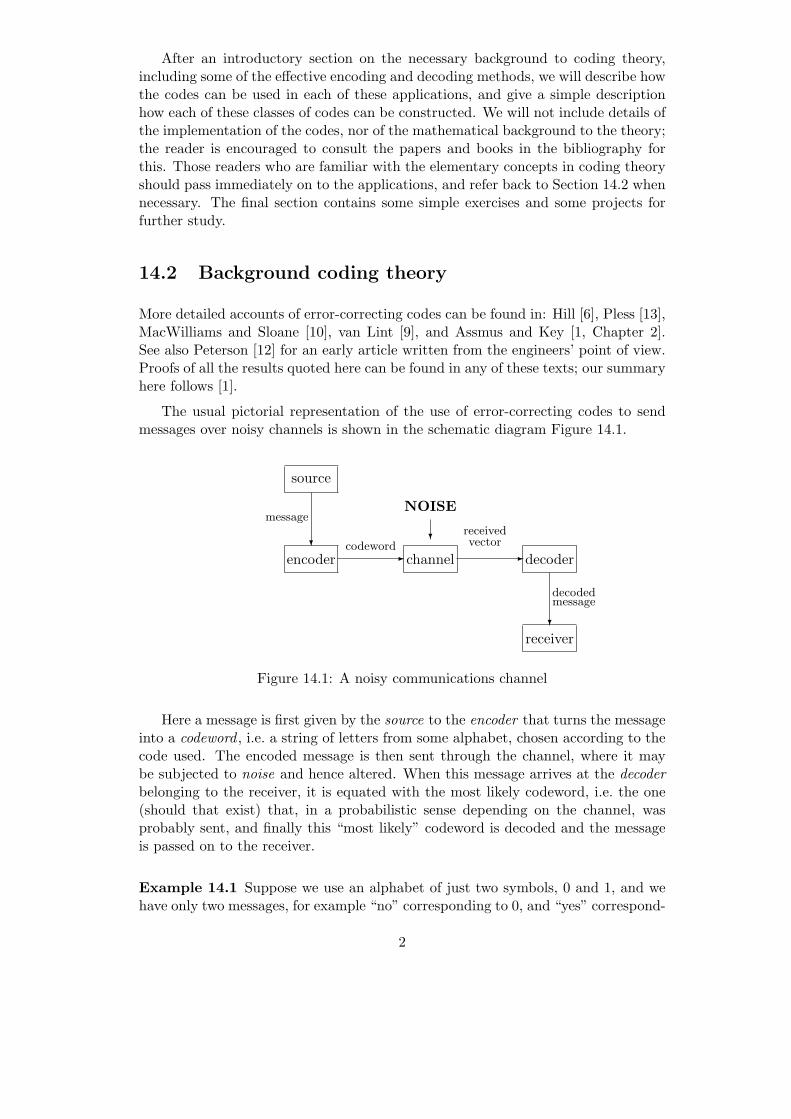
The usual pictorial representation of the use of error-correcting codes to sendmessages over noisy channels is shown in the schematic diagram Figure 14.1.

source

?

message

encoder -codeword

channel

NOISE

?

-

receivedvector

decoder

?

decodedmessage

receiver

Figure 14.1: A noisy communications channel

Here a message is first given by the source to the encoder that turns the messageinto a codeword , i.e. a string of letters from some alphabet, chosen according to thecode used. The encoded message is then sent through the channel, where it maybe subjected to noise and hence altered. When this message arrives at the decoderbelonging to the receiver, it is equated with the most likely codeword, i.e. the one(should that exist) that, in a probabilistic sense depending on the channel, wasprobably sent, and finally this “most likely” codeword is decoded and the messageis passed on to the receiver.

Example 14.1 Suppose we use an alphabet of just two symbols, 0 and 1, and wehave only two messages, for example “no” corresponding to 0, and “yes” correspond-

2

ing to 1. We wish to send the message “no”, and we add redundancy by simplyrepeating the message five times. Thus we encode the message as the codeword(00000). The channel might interfere with the message and could change it to, say,(10100). The decoder assesses the message and decides that of the two possiblecodewords, i.e. (00000) and (11111), the former is the more likely, and hence themessage is decoded, correctly, as “no”.

We have made several assumptions here: for example we have assumed that theprobability of an error at any position in the word is less than 1

2 , that each codewordis equally likely to be sent, and that the receiver is aware of the code used.

Definition 14.1 Let F be a finite set, or alphabet, of q elements. A q-arycode C is a set of finite sequences of symbols of F , called codewords and writtenx1x2 . . . xn, or (x1, x2, . . . , xn), where xi ∈ F for i = 1, . . . , n. If all the sequenceshave the same length n, then C is a block code of block length n.

The code used in the example above is a block code, called the repetition codeof length 5: it can be generalized to length n and to any alphabet of size q, andhence will have q codewords of the form xx · · ·x, where x ∈ F .

Given an alphabet F , it will be convenient, and also consistent with terminologyfor cartesian products of sets and for vector spaces when F is a field, to denote theset of all sequences of length n of elements of F by Fn and to call these sequencesvectors, referring to the member of F in the i th position as the coordinate at i. Weuse either notation, x1x2 · · ·xn or (x1, x2, . . . , xn), for the vectors. A code over F ofblock length n is thus any subset of Fn.

The formal process in the reasoning of the simple example given above uses theconcept of the distance between codewords.

Definition 14.2 Let v = (v1, v2, . . . , vn) and w = (w1, w2, . . . , wn) be two vectors inFn. The Hamming distance, d(v, w), between v and w is the number of coordinateplaces in which they differ:

d(v, w) = |{i|vi 6= wi}|.

We will usually refer to the Hamming distance as simply the distance betweentwo vectors. It is simple to prove that the Hamming distance defines a metric onFn, i.e.

(1) d(v, w) = 0 if and only if v = w;

(2) d(v, w) = d(w, v) for all v, w ∈ Fn;

(3) d(u, w) ≤ d(u, v) + d(v, w) for all u, v, w ∈ Fn.

Nearest-neighbor decoding picks the codeword v′ nearest (in terms of Ham-ming distance) to the received vector, should such a vector be uniquely determined.This method maximizes the decoder’s likelihood of correcting errors — provided

3

that each symbol has the same probability (less than 12) of being received in error

and each symbol of the alphabet is equally likely to occur. A channel with thesetwo properties is called a symmetric q-ary channel.

Definition 14.3 The minimum distance d(C) of a code C is the smallest of thedistances between distinct codewords; i.e.

d(C) = min{d(v, w)|v, w ∈ C, v 6= w}.

For the repetition code of length 5 given in Example 14.1 this distance is 5.

The following simple result is very easily proved and shows the vital importanceof this concept for codes used in symmetric channels.

Theorem 14.1 If d(C) = d then C can detect up to d − 1 errors or correct up tob(d− 1)/2c errors.

(Here bnc denotes the floor function of n.) Thus in Example 14.1 up to fourerrors can be detected or up to two errors can be corrected.

If C is a code of block length n having M codewords and minimum distanced, then we say that C is an (n, M, d) q-ary code, where |F | = q. We will referto n as the length of the code rather than the block length. Thus the code inExample 14.1 is a (5, 2, 5) 2-ary (binary) code.

From the above discussion, we see that for a good (n, M, d) code C, i.e. one thatdetects or corrects many errors, we need d to be large. However we also prefer n tobe small (for fast transmission) and M to be large (for a large number of messages).These are clearly conflicting aims, since for a q-ary code, M ≤ qn. In fact there aremany bounds connecting these three parameters, one of the simplest of which is theSingleton bound (see, for example, [1, Theorem 2.1.2]):

M ≤ qn−d+1. (14.1)

Another bound, usually better than the Singleton bound, is the sphere-packingbound.

Definition 14.4 Let F be any alphabet and suppose u ∈ Fn. For any integerr ≥ 0, the sphere of radius r with center u is the set of vectors Sr(u) = {v|v ∈Fn, d(u, v) ≤ r}.

Let C be an (n, M, d) code. Then the spheres of radius ρ = b(d − 1)/2c withcenter in C do not overlap, i.e. they form M pairwise disjoint subsets of Fn. Theinteger ρ is called the packing radius of C. Hence we have the sphere-packingbound: if C is an (n, M, d) q-ary code of packing radius ρ, then

M

(1 + (q − 1)n + (q − 1)2

(n

2

)+ · · ·+ (q − 1)ρ

(n

ρ

))≤ qn. (14.2)

4

The covering radius of a code is defined to be the smallest integer R such thatspheres of radius R with their centers at the codewords cover all the words of Fn. Ifthe covering radius R is equal to the packing radius ρ, the code is called a perfectρ-error-correcting code. Thus perfect codes are those for which equality holdsin (14.2)

The binary (i.e. |F | = 2) repetition codes of odd length n are trivial perfect(n−1)/2-error-correcting codes; the infinite class of binary perfect 1-error-correctingcodes with n = 2m − 1 and hence M = 2n−m was discovered by Hamming [4] andgeneralized to the q-ary case by Golay.

A code C over the finite field F = Fq of prime-power order q, of length n islinear if C is a subspace of V = Fn. If dim(C) = k and d(C) = d, then we write[n, k, d ] or [n, k, d ]qfor the q-ary code C; if the minimum distance is not specified wesimply write [n, k]. The information rate is k/n and the redundancy is n− k.

Thus a q-ary linear code is any subspace of a finite-dimensional vector spaceover a finite field Fq, but with reference to a particular basis. The standard basisfor Fn, as the space of n-tuples, has a natural ordering through the numbers 1 to n,and this coincides with the spatial layout of a codeword as a sequence of alphabetletters sent over a channel. To avoid ordering the basis we may take V = FX , theset of functions from X to F , where X is any set of size n. Then a linear code isany subspace of V .

For any vector v = (v1, v2, . . . , vn) ∈ V = Fn, let S = {i | vi 6= 0}; then Sis called the support of v, written Supp(v), and the weight of v, wt(v), is |S|.The minimum weight of a code is the minimum of the weights of the non-zerocodewords, and for linear codes is easily seen to be equal to d(C).

For linear [n, k, d ] q-ary codes the Singleton bound and the Sphere-packingbound become the following:

Singleton bound: d ≤ n− k + 1;

sphere-packing bound:∑ρ

i=0(q − 1)i(n

i

)≤ qn−k.

A code for which equality holds in the Singleton bound is called an MDS (maximumdistance separable) code. The Reed-Solomon codes (see Section 14.5.2) are MDScodes.

Definition 14.5 Two linear codes in Fn are equivalent if each can be obtainedfrom the other by permuting the coordinate positions in Fn and multiplying eachcoordinate by a non-zero field element. The codes will be said to be isomorphic ifa permutation of the coordinate positions suffices to take one to the other.

In terms of the distinguished basis that is present when discussing codes, codeequivalence is obtained by reordering the basis and multiplying each of the basiselements by a non-zero scalar. Thus the codes C and C ′ are equivalent if there is alinear transformation of the ambient space Fn, given by a monomial matrix (onenon-zero entry in each row and column) in the standard basis, that carries C ontoC ′. When the codes are isomorphic, a permutation matrix can be found with this

5

property. When q = 2, the two concepts are identical. Clearly equivalent linearcodes must have the same parameters [n, k, d ].

If C is a q-ary [n, k] code, a generator matrix for C is a k × n array obtainedfrom any k linearly independent vectors of C.

Via elementary row operations, a generator matrix G for C can be brought intoreduced row echelon form and still generate C, and then, by permuting columns, itcan be brought into a standard form

G′ = [Ik|A] (14.3)

where this is now a generator matrix for an equivalent (in fact, isomorphic) code.Here A is a k × (n− k) matrix over F .

Now we come to another important way of describing a linear code, viz.through its orthogonal or dual. For this we need an inner product defined onour space; it is the standard inner product: for v, w ∈ Fn, v = (v1, v2, . . . , vn),w = (w1, w2, . . . , wn), we write the inner product of v and w as (v, w) where

(v, w) =n∑

i=1

viwi. (14.4)

Definition 14.6 Let C be a q-ary [n, k] code. The orthogonal code (or dualcode) is denoted by C⊥ and is given by

C⊥ = {v ∈ Fn|(v, c) = 0 for all c ∈ C}.

We call C self-orthogonal if C ⊆ C⊥ and self-dual if C = C⊥.

From elementary linear algebra we have

dim(C) + dim(C⊥) = n (14.5)

since C⊥ is simply the null space of a generator matrix for C. Taking G to be agenerator matrix for C, a generator matrix H for C⊥ satisfies GHt = 0, i.e. c ∈ Cif and only if cHt = 0, or, equivalently, Hct = 0. Any generator matrix H for C⊥ iscalled a parity-check or check matrix for C. If G is written in the standard form

[Ik|A],

thenH = [−At|In−k] (14.6)

is a check matrix for the code with generator matrix G.

In Example 14.1, which is a linear [5, 1, 5]2 code, we have generator matrix

G = [1, 1, 1, 1, 1],

already in standard form, and thus

H =

1 1 0 0 01 0 1 0 01 0 0 1 01 0 0 0 1

6

as a check matrix.

A generator matrix in standard form simplifies encoding: suppose data con-sisting of qk messages are to be encoded by adding redundancy using the code Cwith generator matrix G. First identify the data with the vectors in F k, whereF = Fq. Then for u ∈ F k, encode u by forming uG. If u = (u1, u2, . . . , uk)and G has rows R1, R2, . . . , Rk, where each Ri is in Fn, then uG =

∑i uiRi =

(x1, x2, . . . , xk, xk+1, . . . , xn) ∈ Fn, which is now encoded. But when G is in stan-dard form, the encoding takes the simpler form

u 7→ (u1, u2, . . . , uk, xk+1, . . . , xn),

and here the u1, . . . , uk are the message or information symbols, and the last n− kentries are the check symbols, and represent the redundancy.

In general it is not possible to say anything about the minimum weight of C⊥

knowing only the minimum weight of C but, of course, either a generator matrix ora check matrix gives complete information about both C and C⊥. In particular, acheck matrix for C determines the minimum weight of C in a useful way:

Theorem 14.2 Let H be a check matrix for an [n, k, d ] code C. Then every choiceof d− 1 or fewer columns of H forms a linearly independent set. Moreover if everyd−1 or fewer columns of a check matrix for a code C are linearly independent, thenthe code has minimum weight at least d.

Notice that in terms of generator matrices, two codes C and C ′ with generatormatrices G and G′ are equivalent if and only if there exist a non-singular matrixM and a monomial matrix N such that MGN = G′, with isomorphism if N is apermutation matrix and equality if N = In, n being the block length of the codes.

Example 14.2 The smallest non-trivial Hamming code (see Section 14.3.2) is a[7,4,3] binary code, which is a perfect single-error-correcting code. It can be givenby the generator matrix G in standard form [I4|A] where

A =

1 1 10 1 11 0 11 1 0

.

Thus a check matrix will be

H =

1 0 1 1 1 0 01 1 0 1 0 1 01 1 1 0 0 0 1

.

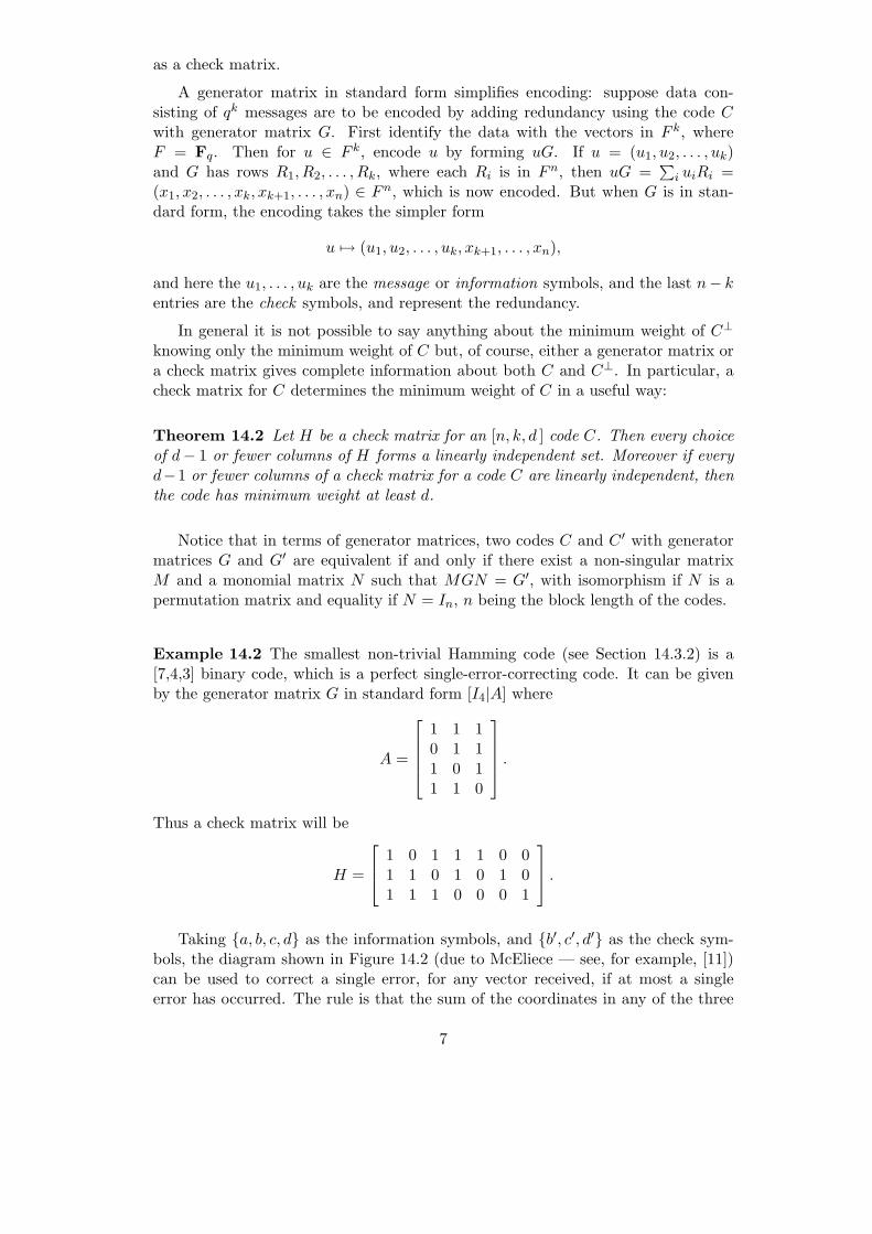
Taking {a, b, c, d} as the information symbols, and {b′, c′, d′} as the check sym-bols, the diagram shown in Figure 14.2 (due to McEliece — see, for example, [11])can be used to correct a single error, for any vector received, if at most a singleerror has occurred. The rule is that the sum of the coordinates in any of the three

7

&%'$

&%'$&%

'$c

d

ba

b′ c′

d′

Figure 14.2: The Hamming code H3

circles must be 0, which constitute the “parity checks” as seen from the matrix Habove. Thus, for example, if the vector 1011111 is received, checking the parity inthe three circles shows that an error occurred at the information symbol b, so thatthe error is corrected, yielding 1111111.

A general method of decoding for linear codes is a method, due to Slepian [15],that uses nearest-neighbor decoding and is called standard-array decoding. Theerror vector is defined to be e = w− v, where v is the codeword sent and w is thereceived vector. Given the received vector we wish to determine the error vector.We look for that coset of the subgroup C in Fn that contains w and observe thatthe possible error vectors are just the members of this coset. The strategy is thus tolook for a vector e of minimum weight in the coset w + C, and decode as v = w− e.A vector of minimum weight in a coset is called a coset leader; of course it mightnot be unique, but it will be in the event that its weight is at most ρ, where ρ isthe packing radius, and this will always happen when at most ρ errors occurredduring transmission. It should be noted that there may be a unique coset leadereven when the weight of that leader is greater than ρ and thus a complete analysisof the probability of success of nearest-neighbor decoding will involve analyzing theweight distribution of all the cosets of C; in the engineering literature this is knownas “decoding beyond the minimum distance”. Use of a parity-check matrix H for Cto calculate the syndrome, viz.

synd(w) = wHt, (14.7)

of the received vector w assists this decoding method, the syndrome being constantover a coset and equal to the zero vector when a codeword has been received.

Definition 14.7 Let C be a q-ary [n, k, d ] code. Define the extended code C to bethe code of length n + 1 in Fn+1 of all vectors c for c ∈ C where, if c = (c1, . . . , cn),then

c =

(c1, . . . , cn,−

n∑i=1

ci

).

This is called adding an overall parity check, for we see that if v =(v1, . . . , vn+1) then v ∈ C satisfies

∑vi = 0. If C has generator matrix G and

check matrix H, then C has generator matrix G and check matrix H, where G isobtained from G by adding an (n+1)th column such that the sum of the columns ofG is the zero column, and H is obtained from H by attaching an (n−k+1)th row and(n+1)th column onto H, the row being all 1’s and the column being (0, 0, . . . , 0, 1)t.If C is binary with d odd, then C will be an [n + 1, k, d + 1] code.

8

Example 14.3 Extending the [7, 4, 3] binary Hamming code gives an [8, 4, 4] binarycode, which is self-dual.

An inverse process to extending an [n, k, d ] code is that of puncturing, whichis achieved by simply deleting a coordinate, thus producing a linear code of lengthn− 1. The dimension will be k or k − 1, clearly, but in the great majority of casesthe dimension will remain k; the minimum weight may change in either way, butunless the minimum weight of the original code is 1, the minimum weight of thepunctured code will be either d− 1 or d and in the great majority of cases d− 1.

Another way to obtain new codes is by shortening: given an [n, k, d] q-ary codeC, for any integer r ≤ k, we take the subspace C ′ of all codewords having 0 in a fixedset of r coordinate positions, and then remove those coordinate positions to obtaina code of length n − r. For example, if G is a generator matrix for C in standardform, shortening by the first coordinate will clearly produce an [n−1, k−1, d′] code,where d′ ≥ d. In this way we obtain [n− r, k − r, d′] codes. This techinique is usedin Section 14.5.

14.3 Computer memories and Hamming codes

14.3.1 Introduction

Before going on to defining the actual codes, we describe briefly how the memorychips are designed, and how codes may be used, and why they are needed. A fulleraccount of the use of error-correcting codes in computer memories may be found inthe article [11].

The memories of computers are built from silicon chips. Although any one ofthese chips is reliable, when many thousands are combined in a memory, some mightfail. The use of an error-correcting code can mean that a failed chip will be detectedand the error corrected. The errors in a chip might occur in the following way: amemory chip is a square array of data-storage cells, for example a 64K chip, whereK = 210. The 64K chip stores 64K = 216 = 65, 536 bits, i.e. binary digits, of data.Alternatively, there are 256K = 218 and one-megabit (220 bits) chips. In the 64Kchip the data-storage cells are arranged in a 28× 28 array, where each cell stores a 0or a 1. Each cell can be accessed individually, and has an “address” correspondingto the row and column coordinates, usually numbered from 0 to 255. The largestaddress is in position (255, 255) = (28 − 1, 28 − 1); the binary representation of 255is 11111111, a sequence of eight bits, and thus the row and column addresses fora 64K require eight bits each, i.e. 16 in all. A 256K chip has 29 = 512 rows andcolumns and thus requires 18 bits to address a cell, and a one-megabit chip requires20.

The 0’s or 1’s stored in a memory chip are represented by the presence or absenceof negative electric charges at sites in the silicon crystal whose electrical propertiesmake them potential wells for negative charge. When a 0 is to be stored in a cellthe potential well at the site is filled with electrons; when a 1 is to be stored thewell is emptied. The cell is read by measuring its negative charge; if the charge is

9

higher than a certain value it is read to be a 0, otherwise a 1.

Clearly, if a potential well lost its charge it would be read incorrectly. Errors dooccur: hard errors occur when the chip itself is damaged; soft errors occur whenthe chip itself is not damaged but alpha particle bombardment occurs and changesthe charge in a cell. The latter is a common cause of error and cannot be avoided.

An error-correcting code is used to correct such errors in the following way:suppose we have a one megabyte memory consisting of 128 64K chips. In such amemory the chips are arranged in four rows of 32 chips each; each chip contains216 memory cells, so the memory has a total of 223 cells. The data are divided intowords of 32 bits each, and each word consists of the contents of one memory cell ineach of the 32 chips in one row. In order to correct errors, a further seven chips areadded to each of the four rows, making 156 chips. Each row has now 39 chips, theseven extra bit being the parity bits, and are reserved for error-correction. The codeactually employed is the binary extended Hamming code of length 64, i.e. a [64, 57, 4]binary code. Such a code will actually protect 57 bits of data, but designers of thecodes use only 32 bits.

We now describe how the (binary) Hamming codes are defined.

14.3.2 Hamming codes

These codes were first fully described by Golay [3] and Hamming [4, 5] althoughthe [7, 4] binary code had already appeared in Shannon’s fundamental paper. Theyprovide an infinite class of perfect codes. We need here only the binary case, whichwas the one considered by Hamming. Consider a binary code C with check matrixH: the transposed syndrome, Hyt, of a received vector y is, in the binary case,simply the sum of those columns of H where the errors occurred. To design asingle-error-correcting code we want H not to have any zero columns, since errorsin that position would not be detected; similarly, we want H not to have any equalcolumns, for then errors in those positions would be indistinguishable. If such anH has r rows, n columns and is of rank r, then it will be a check matrix for asingle-error-correcting [n, n − r] code. Thus, to maximize the dimension, n shouldbe chosen as large as possible. The number of distinct non-zero r-tuples availablefor columns is 2r − 1. We take for H the r× (2r − 1) binary matrix whose columnsare all the distinct non-zero r-tuples.

Definition 14.8 The binary Hamming code of length 2r−1 is the code Hr that hasfor check matrix the r × (2r − 1) matrix H of all non-zero r-tuples over F2.

Theorem 14.3 The binary code Hr is a [2r − 1, 2r − 1− r, 3] perfect single-error-correcting code for all r ≥ 2.

Example 14.4 (1) If r = 2 then

H =

[1 0 10 1 1

]

10

and H2 is a [3, 1, 3] code, which is simply the binary repetition code of length3.

(2) If r = 3, H3 is a [7, 4, 3] binary code, with check matrix

H =

1 0 1 0 1 0 10 1 1 0 0 1 10 0 0 1 1 1 1

.

Decoding a binary Hamming code is very easy. We first arrange the columnsof H, a check matrix for Hr, so that the j th column represents the binary repre-sentation (transposed) of the integer j. Now we decode as follows. Suppose thevector y is received. We first find the syndrome, synd(y) = yHt. If synd(y) = 0,then decode as y, since then y ∈ Hr. If synd(y) 6= 0, then, assuming one error hasoccurred, it must have occurred at the j th position where the vector (synd(y))t isthe binary representation of the integer j. Thus decode y to y + ej , where ej is thevector of length n = 2r − 1 with 0 in every position except the j th, where it has a1. The examples given here use this ordering, but notice that the ordering of theentries in the transposed m-tuple representing a number is read from left to right.Thus, [1011] (transposed) represents 1 + 0 + 4 + 8 = 13 rather than the customary1 + 2 + 0 + 8 = 11.

If we form the extended binary Hamming code Hr, we obtain a [2r, 2r − 1− r, 4]code which is still single-error-correcting, but which is capable of simultaneouslydetecting two errors. This code is useful for incomplete decoding : see Hill [6].

Example 14.5 Let C = H3, with check matrix H obtained as described above (seeafter Definition 14.7):

H =

1 0 1 0 1 0 1 00 1 1 0 0 1 1 00 0 0 1 1 1 1 01 1 1 1 1 1 1 1

,

and generator matrix

G =

1 1 1 0 0 0 0 11 0 0 1 1 0 0 10 1 0 1 0 1 0 11 1 0 1 0 0 1 0

.

The data set (1, 0, 1, 0) is encoded as (1, 0, 1, 0)G = (1, 0, 1, 1, 0, 1, 0, 0). If a singleerror occurs at the i th position, then the received vector y will have (synd(y))t thei th column of H and decoding can be performed. However, if two errors occur, atthe i th and j th positions, the (synd(y))t will be the sum of the i th and j th columnsof H, and thus will have 0 as the last entry. Decocoding will thus not take place.

Definition 14.9 The orthogonal code H⊥r of Hr is called the binary simplex code

and is denoted by Sr.

11

The simplex code Sr clearly has length 2r − 1 and dimension r. The generatormatrix is H. It follows that Sr consists of the zero vector and 2r − 1 vectors ofweight 2r−1, so that it is a [2r − 1, r, 2r−1] binary code. Any two codewords areat Hamming distance 2r−1 and, if the codewords are placed at the vertices of aunit cube in 2r − 1 dimensions, they form a simplex. Now from elementary codingtheory (see Section 2) we know that a check matrix for Hr is H with a column ofzeros attached, and then a further row with all entries equal to 1: the code spannedby this matrix, i.e. Hr

⊥, is a [2r, r + 1, 2r−1] binary code, and is also a first-order

Reed-Muller code, denoted by R(1, r). It can correct 2r−2 − 1 errors.

Finally now, looking back at the application to computer memories, the codeused is H6, a [64, 57, 4] binary code. A check matrix can easily be constructed inthe manner described above. The code will now correct any single error that occursin the way described above, and will simultaneously detect any two errors.

14.4 Photographs in space and Reed-Muller codes

14.4.1 Introduction

Photographs of the planet Mars were first taken by the Mariner series of spacecraft inthe ’60s and early ’70s and the first-order Reed-Muller code of length 32 was used toobtain good quality photographs. The original black and white photographs takenby the earlier Mariners were broken down into 200 × 200 picture elements. Eachelement was assigned a binary 6-tuple representing one of 64 possible brightnesslevels from, say, 000000 for white to 111111 for black. Later this division was madefiner by using 700× 832 elements, and the quality was increased by encoding the 6-tuples using the [32, 6, 16] binary 7-error correcting Reed-Muller code R(1, 5) in theway described in Section 14.2. When color photographs were taken, the same codewas used simply by using the same photograph through different colored filters. Inthe Voyager series after the late ’70s the binary extended Golay code G24, a [24, 12, 8]code, was used in the color photography.

Later on in the Voyager series of spacecraft a different type of codes, viz. con-volutional Reed-Solomon codes, was used: see [17]. We describe the Reed-Solomoncodes in Section 14.5.2.

14.4.2 First-order Reed-Muller codes

A full account of the Reed-Muller codes, which are all binary codes, can be foundin [10] or [1, Chapter 5]. We describe here simply a way to construct the [32, 6, 16]code used for space photography, although in fact we can be more general sincewe already have the construction from the extended Hamming codes. Thus wehave the first-order Reed-Muller code R(1,m) of length 2m is the code Hm

⊥, i.e.

the orthogonal of the extended binary Hamming code. It is, as discussed above, a[2m,m+1, 2m−1] binary (2m−2−1)-error-correcting code. A 6×32 generator matrixG for R(1, 5) may thus be constructed as follows: first form a 5×31 matrix G0 withcolumns the binary representation of each number between 1 and 31 as a column

12

of length 5; then adjoin a column with all entries zero, and finally add a sixth rowwith all entries equal to 1. Thus

G0 =

1 0 1 · · · 0 10 1 1 · · · 1 10 0 0 · · · 1 10 0 0 · · · 1 10 0 0 · · · 1 1

and

G =

0

G0...0

1 1 1 · · · 1

.

14.4.3 The binary Golay codes

There are many ways to arrive at the perfect Golay [23, 12, 7] binary 3-error-correcting code G23 and its extension, the [24, 12, 8] binary Golay code G24 thatwas used in the Voyager spacecraft. We will give a generator matrix, as Golayoriginally did in [3]. That the code generated by this matrix has the specified prop-erties can be verified very easily, or by consulting any of the references given inSection 14.2, for example [6, Chapter 9].

A generator matrix over F2 for G24 is

G = [I12|B], (14.8)

where I12 is the 12× 12 identity matrix and B is a 12× 12 matrix given by

B =

0 1 · · · 11... A1

, (14.9)

where A is an 11 × 11 matrix of 0’s and 1’s defined in the following way: considerthe finite field F11 of order 11, i.e. the eleven remainders modulo 11. The first rowof A is labelled by these eleven remainders in order, starting with 0, and placing anentry 1 in the ith position if i is a square modulo 11, and a 0 otherwise. The squaresmodulo 11 are {0, 1, 3, 4, 5, 9}, and thus the first row of A is

[1 1 0 1 1 1 0 0 0 1 0

].

13

For the remaining rows of A simply cycle this row to the left ten times, to obtain

A =

1 1 0 1 1 1 0 0 0 1 01 0 1 1 1 0 0 0 1 0 10 1 1 1 0 0 0 1 0 1 11 1 1 0 0 0 1 0 1 1 01 1 0 0 0 1 0 1 1 0 11 0 0 0 1 0 1 1 0 1 10 0 0 1 0 1 1 0 1 1 10 0 1 0 1 1 0 1 1 1 00 1 0 1 1 0 1 1 1 0 01 0 1 1 0 1 1 1 0 0 00 1 1 0 1 1 1 0 0 0 1

. (14.10)

(This construction is quite general in fact and leads to a class of Hadamardmatrices and also to the quadratic residue codes: see [1, Chapters 2,7] for furtherdetails.) An effective decoding algorithm for G24 is given in [16, Chapter 4].

The perfect binary Golay code G23 may be obtained from G24 by deleting anycoordinate.

14.5 Compact discs and Reed-Solomon codes

14.5.1 Introduction

A full account of the use of Reed-Solomon codes for error-correction in compactdiscs is given in [7], [16, Chapter 7] or [17].

Sound is stored on a compact disc by dividing it up into small parts and rep-resenting these parts by binary data, just as pictures are divided up, as describedin Section 14.4. A compact disc is made by sampling sound waves 44,100 times persecond, the amplitude measured and assigned a value between 1 and 216 − 1, givenas a binary 16-tuple. In fact, two samples are taken, one for the left and one for theright channel. Each binary 16-tuple is taken to represent two field elements fromthe Galois field of 28 elements, F28 , and thus each sample produces four symbolsfrom F28 .

For error-correction the information is broken up into segments called frames,where each frame holds 24 data symbols. The code used for error-correction is aCross Interleaved Reed-Solomon code (CIRC) obtained by a process called “cross-interleaving” of two shortened Reed-Solomon codes, as described below. The 24symbols from F28 from six samples are used as information symbols in a (short-ened) Reed-Solomon [28, 24, 5] code C1 over F28 . Another shortened Reed-Solomon[32, 28, 5] code C2 also over F28 is then used in the interleaving process, which hasfour additional parity-check symbols. See [7, 16, 17] for a detailed description ofthis process.

As a result of this interleaving process of error-correction, flaws such as scratcheson a disc, producing a train of errors called an “error burst”, can be corrected.

14

We describe now the basic Reed-Solomon class of codes.

14.5.2 Reed-Solomon codes

The Reed-Solomon codes are a class of cyclic q-ary codes of length n dividing q − 1that satisfy the Singleton bound, and are thus also MDS codes (see Section 14.2). Itwould take too long to describe general cyclic codes, but we will nevertheless definethese codes as being cyclic and illustrate immediately how a generator matrix anda check matrix may be found.

Let F = Fq and let n|(q − 1). Then F has elements of order n, and we let β besuch an element. Pick any number δ such that 2 ≤ δ ≤ n, and take any number asuch that 0 ≤ a ≤ q − 2. Then the polynomial

g(X) = (X − β1+a)(X − β2+a)(X − β3+a) . . . (X − βδ−1+a) (14.11)

is the generator polynomial of an [n, n − δ + 1, δ] code over F , a Reed-Solomoncode. In the special case when n = q−1 the code is a primitive Reed-Solomon code.We obtain a generator polynomial for the code by first expanding the polynomialg(X) to obtain, writing d = δ (since δ is indeed the minimum weight),

g(X) = g0 + g1X + · · ·+ gd−2Xd−2 + Xd−1 (14.12)

where gi ∈ F for each i. A generator matrix can then be shown to be

G =

g0 g1 g2 . . . gd−1 1 0 . . . 00 g0 g1 . . . gd−2 gd−1 1 . . . 0...

.... . .

......

......

. . ....

0 . . . . . . g0 . . . . . . gd−2 gd−1 1

. (14.13)

The general theory of BCH codes (see [1, Chapter 2]) immediately gives a checkmatrix

H =

1 β β2 . . . β(n−1)

1 β2 β4 . . . β2(n−1)

......

......

1 βd−1 β2(d−1) . . . β(n−1)(d−1)

, (14.14)

taking here a = 0. This is a convenient generator matrix for the orthogonal code(which is also a Reed-Solomon code) with a rather simple encoding rule: the dataset (a1, a2, . . . , ad−1) is encoded as (a(1), a(β), a(β2), . . . , a(βn−1)) where

a(X) = a1X + a2X2 . . . ad−1X

d−1.

The theory (see [1, Chapter 2]) also tells us that the reciprocal polynomial ofh(X) = (Xn − 1)/g(X), i.e. h(X) = Xn−d+1h(X−1), is a generator polynomial forthe orthogonal code, so another check matrix may be obtained for this in the sameway as we did for the code with g(X) as generator polynomial. A more convenientmethod for the purposes here is to reduce G to standard form and then simply usethe formula shown in Equation (14.6).

15

Example 14.6 Let q = 11 and n = 5. Then we can take β = 4 as this has orderprecisely 5, and let a = 0 and δ = 3. Then

g(X) = (X − β)(X − β2) = (X − 4)(X − 5) = 9 + 2X + X2

so that

G =

9 2 1 0 00 9 2 1 00 0 9 2 1

.

Since (X5 − 1) = (X − 1)(X − 4)(X − 5)(X − 9)(X − 3), (X5 − 1)/g(X) = (X −1)(X − 3)(X − 9) and the orthogonal code has generator polynomial

h(X) = X3(X−1 − 1)(X−1 − 3)(X−1 − 9) = 1 + 9X + 6X2 + 6X3,

so that a check matrix is

H =

[1 9 6 6 00 1 9 6 6

].

Alternatively, the check matrix can be obtained from Equation (14.14), giving

H ′ =

[1 4 5 9 31 5 3 4 9

],

which is of course row-equivalent to H.

The codes used are actually shortened Reed-Solomon codes (see Section 14.2).The easiest way to describe these codes is to have a generator matrix of the originalReed-Solomon code C in standard form, which is possible without even havingto take an isomorphic code in this case, due to the Reed-Solomon codes havingthe property of being MDS codes. Thus a generator matrix can be row reducedto standard form, without the need of column operations. (Sometimes it is moreconvenient to use the standard form for the orthogonal code rather, and thus havethe generator matrix in the form [A|Ik].) If now C, an [n, k, d] q-ary code withn− k = d− 1, is to be shortened in the first r places to obtain a code C ′ of lengthn − r, we obtain a generator matrix G′ for C ′ also in standard form by simplydeleting the first r rows and columns of G. If H is the check matrix in standardform for G, then the check matrix in standard form for G′ is H ′ obtained from Hby deleting the first r columns. It is easy to see that the MDS properties of theoriginal code show that C ′ is also MDS and is an [n− r, k− r, d] q-ary code, and, ofcourse, n− r = k − r + d− 1.

The finite field used in the codes used for compact discs is the field F = F28 oforder 28. This can be constructed as the set of all polynomials over the field F2 ofdegree at most 7, i.e.

F = {a0 + a1X + a2X2 + a3X

3 + a4X4 + a5X

5 + a6X6 + a7X

7 : ai ∈ F2}.

Addition of these polynomials is just the standard addition, as is multiplication,except that multiplication is carried out modulo the polynomial

1 + X2 + X3 + X4 + X8. (14.15)

16

Thus X8 = 1 + X2 + X3 + X3 and all other powers of X are reduced to be at most7, using this rule. The elements of F = F28 are thus effectively 8-tuples of binarydigits, and this is how they are treated for the application.

The length of the Reed-Solomon codes over F are divisors of 28 − 1 = 255 =3× 5× 17. The code actually used is the shortened primitive one, i.e. the shortened[255, 251, 5] code over F , with certain information symbols set to zero. Then if ω isa primitive element for the field (i.e. an element of multiplicative order 255), we takeβ = ω. Since we want minimum distance 5, we take k = n − 4 = 251, and shortento length 28 for C1 and to length 32 for C2. The original Reed-Solomon of length255 would be the same for the two codes, and would have generator polynomial

g(X) = (X − ω)(X − ω2)(X − ω3)(X − ω4) = ω10 + ω81X + ω251X2 + ω76X3 + X4.

The powers of ω are then given as binary 8-tuples: for example,

ω10 = ω2 + ω4 + ω5 + ω6 = (0, 0, 1, 0, 1, 1, 1, 0),

andω251 = ω3 + ω4 + ω6 + ω7 = (0, 0, 0, 1, 1, 0, 1, 1),

as can be computed using, for example, the computer package Magma [2].

For further details of the properties of finite fields, the reader might consult [8].

14.6 Conclusion

We have been brief in this outline of the use of well-known mathematical construc-tions in important practical examples, and have not included full details of theimplementation of the codes. The reader is urged to consult the bibliography in-cluded here for a full and detailed description of the usage. We hope merely to havegiven some idea as to the nature of the codes, and where they are applied.

The exercises included in the next section should be accessible using the defi-nitions described in this chapter. They are mostly quite elementary. The projectsdescribed are open problems whose solution might prove to have rather importantapplications; some computational results might first be done to make the questionsmore precise, in particular in the case of Project 2. Magma [2] is a good computa-tional tool to use for this type of problem.

14.7 Exercises and projects

EXERCISES

1. Prove Theorem 14.1.

2. If C is a code of packing radius ρ, show that the spheres with radius ρ andcenters the codewords of C do not intersect. Hence deduce the sphere packingbound, Equation 14.2.

17

3. Prove Theorem 14.2.

4. Let C be a binary code with generator matrix

G =

[1 0 1 1 01 1 0 1 1

].

Show that d(C) = 3 and construct a check matrix for C. If a vector y =(0, 1, 1, 1, 1) were received, what would you correct it to?

5. State the Singleton bound and the sphere packing bound for an (n, M, d) q-ary code. Compare these to find the best bound for M for a (10,M, 5) binarycode.

6. A linear code C is self-orthogonal if C ⊆ C⊥. Let C be a binary code. Showthat

(a) if C is self-orthogonal then every codeword has even weight;

(b) if every codeword of C has weight divisible by 4 then C is self-orthogonal;

(c) if C is self-orthogonal and generated by a set of vectors of weight divisibleby 4, then every codeword has weight divisible by 4 (i.e. C is doubly-even).

7. Let C be a linear code with check matrix H and covering radius r. Show thatr is the maximum weight of a coset leader for C, and that r is the smallestnumber s such that every syndrome is a linear combination of s or fewercolumns of H.

8. Prove from Definition 14.8 that Hr is a [2r − 1, 2r − 1 − r, 3] perfect binarycode.

9. Use the diagram shown in Figure 14.2 to decode the received vectors 1101101and 1001011.

10. Write down a check matrix for H4, writing the columns so that the jth columnis the binary representation of the number j. Use the method described onpage 11 to decode

∑10i=1 ei and

∑5j=1 e2j−1, where ei is the vector of length 15

with an entry 1 in the ith position, and zeros elsewhere.

11. Show that a binary [23, 12, 7] code is perfect, 3-error-correcting.

12. In the matrix A of Equation (14.10) show that the sum of the first row withany other row has weight 6, and hence that the sum of any distinct two rowsof A has weight 6. What can then be said for the sum of any two rows of B?

13. If C is an [n, k, d] code with generator matrix G in standard form, show thatshortening of C by the first r coordinate positions, where r ≤ k, produces an[n− r, k − r, d′] code C ′ where d′ ≥ d. (Hint: look at the check matrix for C ′

and use Theorem 14.2.) Show that it is possible for d′ > d by constructing anexample.

18

14. Construct a primitive [6, 4, 3] Reed-Solomon code C over F7 using the primitiveelement 3. Form a shortened code of length 4 and determine its minimumdistance.

Extend C to C (see Definition 14.7). Is C also MDS? Give generator matricesfor C and (C)⊥.

15. Construct the Reed-Solomon code of length 16 and minimum distance 5 bygiving its generator polynomial and a check matrix.

PROJECTS

1. Let C be a Hamming code Hr. Is it possible to construct a generator matrixG for C such that every row of G has exactly three non-zero entries, andevery column of G has at most three non-zero entries?

2. Is it possible, in general, to construct a basis of minimum weight vectors forother Hamming and Reed-Muller codes?

19

20

Bibliography

[1] E. F. Assmus, Jr. and J. D. Key. Designs and their Codes. Cambridge Tracts inMathematics, Vol. 103. Cambridge University Press, Cambridge, 1992 (Secondprinting with corrections, 1993).

[2] Wieb Bosma and John Cannon. Handbook of Magma Functions. Departmentof Mathematics, University of Sydney, November 1994.

[3] Marcel J. E. Golay. Notes on digital coding. Proc. IRE, 37:657, 1949.

[4] R. W. Hamming. Error detecting and error correcting codes. Bell System Tech.J., 29:147–160, 1950.

[5] Richard W. Hamming. Coding and Information Theory. Prentice Hall, Engle-wood Cliffs, N.J., 1980.

[6] Raymond Hill. A First Course in Coding Theory. Oxford Applied Mathematicsand Computing Science Series. Oxford University Press, Oxford, 1986.

[7] H. Hoeve, J. Timmermans, and L. B. Vries. Error correction and concealmentin the compact disc system. Philips Tech. Rev., 40:166–172, 1982.

[8] Rudolf Lidl and Harald Niederreiter. Introduction to Finite Fields and theirApplications. Cambridge University Press, Cambridge, 1986.

[9] J. H. van Lint. Introduction to Coding Theory. Graduate Texts in Mathemat-ics 86. Springer-Verlag, New York, 1982.

[10] F. J. MacWilliams and N. J. A. Sloane. The Theory of Error-Correcting Codes.North-Holland, Amsterdam, 1983.

[11] Robert J. McEliece. The reliability of computer memories. Scientific American,252:2–7, 1985.

[12] W. Wesley Peterson. Error-correcting codes. Scientific American, 206:96–108,1962.

[13] Vera Pless. The Theory of Error Correcting Codes. Wiley Interscience Seriesin Discrete Mathematics and Optimization. John Wiley and Sons, New York,1989 (Second Edition.

[14] C. E. Shannon. A mathematical theory of communication. Bell System Tech.J., 27:379–423,623–656, 1948.

21

[15] David Slepian. Some further theory of group codes. Bell System Tech. J.,39:1219–1252, 1960.

[16] Scott A. Vanstone and Paul C. van Oorschot. An Introduction to Error Cor-recting Codes with Applications. Kluwer Academic Publishers, 1992.

[17] Stephen B. Wicker and Vijay K. Bhargava (Editors). Reed-Solomon Codes andtheir Applications. IEEE Press, 1994.

April 22, 2003

22