SOME CRITICAL IMPLEMENTATION ISSUES INITERATIVE ROBUST CONTROL DESIGN

S. Bittanti ∗ M.C. Campi ∗∗ S. Garatti ∗

∗ Dipartimento di Elettronica ed Informazione - Politecnico diMilano, Piazza Leonardo da Vinci 32, 20133 Milano, Italy -

{bittanti,sgaratti}@elet.polimi.it∗∗ Dipartimento di Elettronica per l’Automazione - University of

Brescia,Via Branze 38, 25123 Brescia, Italy -campi@ing.unibs.it

Abstract: Iterative control is an efficient methodology for the design of highly-performingcontrollers. In this paper, we discuss many implementation issues of a new iterativescheme which explicitly accounts for the presence of uncertainty. The developed iter-ative enables one to improve quickly the performance through subsequent steps, whilepreserving the robust stability of the closed-loop system.

Keywords: Iterative methods, robustness, closed-loop identification, Montecarlo method,randomized algorithms

1. INTRODUCTION

The standard paradigm in control design is to work outa suitable controller once a model of the plant is given.When the model cannot be derived from physicalconsiderations, one typically resorts to identificationmethods.In the context of system identification, the one-shotidentification strategy (i.e. the model is first identi-fied and the controller is then designed based on theobtained model) may suffer from drawbacks in caseof high levels of uncertainty, especially for the dif-ficulties inherent in the a-priori selection of a modelclass (see (Gevers, 2000) and (Van den Hof andSchrama, 1995)).In recent years, a great deal of attention has beendevoted to iterative (identification and control) tech-niques. Here, the design is performed with a se-quence of intertwined closed-loop identification andcontrol steps, so as to progressively bring into lightthe plant dynamics and correspondingly improve thecontrol system performance (see (Gevers, 2000), (Leeet al., 1995) and (Van den Hof and Schrama, 1995)).

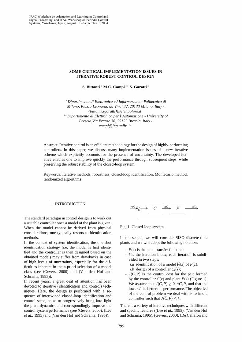
PC y(t)r(t) u(t)+

-

Fig. 1. Closed-loop system.

In the sequel, we will consider SISO discrete-timeplants and we will adopt the following notation:

- P(z) is the plant transfer function;- i is the iteration index; each iteration is subdi-

vided in two steps:i.a identification of a model Pi(z) of P(z);i.b design of a controller Ci(z);

- J(C,P) is the control cost for the pair formedby the controller C(z) and plant P(z) (Figure 1).We assume that J(C,P) ≥ 0, ∀C,P, and that thelower J the better the performance. The objectiveof the control problem we deal with is to find acontroller such that J(C,P) ≤ k.

There is a variety of iterative techniques with differentand specific features ((Lee et al., 1995), (Van den Hofand Schrama, 1995), (Gevers, 2000), (De Callafon and

IFAC Workshop on Adaptation and Learning in Control andSignal Processing, and IFAC Workshop on Periodic ControlSystems, Yokohama, Japan, August 30 – September 1, 2004

795

Van den Hof, 1997)). In the well known “windsurfer"approach ((Lee et al., 1995)) step i.b is split into anumber of sub-steps: namely, starting from the modelidentified at step i.a, the controller is progressivelytuned so as to enlarge the closed-loop bandwidth andat any sub-steps the designed controller is tested onthe real plant to avoid reaching the instability limit.In principle, this is a wise cautious procedure sincein the first iterations the identified model is still ratherunreliable. When it is likely that a further increment inthe bandwidth may lead to instability, one proceeds tothe new iteration i+1 so as to improve the knowledgeon the plant dynamics thanks to a new identificationphase exploiting the data measured from the closed-loop system consisting of {Ci(z),P(z)}, where Ci(z) isthe last controller obtained at the end of the previousiteration. Unfortunately, this way of proceeding mayrequire a number of intermediate steps and a rela-tively long design phase with many experiments onthe real plant. The cautiousness of this approach is afeature shared by other standard iterative schemes (see(Anderson et al., 1998) and (Bitmead et al., 1997)).As discussed in (De Callafon and Van den Hof, 1997)and (Bittanti et al., 2002), a way of alleviating thedrawbacks stemming from the cautiousness of theabove approaches is to resort to robust iterative con-trol techniques, i.e. iterative schemes which explicitlyaccount for the presence of uncertainty in the controldesign phase. Along this robust line, point i.a is splitin two sub-points, and the whole identification-controlprocedure becomes:

i.a from the data collected in closed-loopi.a.1 estimate the nominal model;i.a.2 estimate the model uncertainty;

i.b design the best possible robust controller Ci(z)according to the existing level of uncertainty.Connect it to the plant as in Figure 1;

i.c check the result:i.c.1 if J(Ci,P) ≤ k, then stop.i.c.2 else, put i = i+1 and go to step i.a.

The algorithm is initialized by connecting the plantwith an initial controller C0(z). Typically, due to theuncertainty in the model plant, the performance ofsuch initial control system is poor.The idea behind points i.a and i.b above can be ex-plained as follows. At iteration i, a sensible selectionof the controller has to meet two different and con-trasting objectives:

- on the one hand, the controller has to be cautiousto avoid a possible destabilization of the controlsystem;

- on the other hand, it should not be overconser-vative, otherwise the corresponding performanceimprovement is not significant.

The robust controller design performs in a single stepthe best compromise between the above two objectivesaccording to the present level of uncertainty. In thisway, the achieved performance rapidly improves from

one iteration to the next, while preserving the robuststability of the closed-loop system. This is contrastwith standard iterative schemes, where neglecting un-certainty has the consequence of requiring the splittingof the control design step into a number of sub-steps,with corresponding experimental over-effort.

The iterative algorithm outlined above describes theessential idea of iterative robust control at a generallevel. However, to fill the gap between the generalidea and the real application, one has to decide howto perform the identification and the model qualityestimation (step i.a), and also which kind of robustcontrol method has to be used (step i.b).These points do not seem to be well clarified in the ex-isting literature, though it is apparent that addressingthem is of paramount importance for the success ofthe iterative algorithm. The main goal of this paper isto explicitly discuss the above issues so as to providea complete iterative robust control scheme.Precisely, the estimation of the nominal model andmodel uncertainty in step i.a is discussed in Section 2,while in Section 3 our robust control approach, basedon an average cost criterion, is presented. Then, thecomplete iterative scheme is presented in Section 4,and a simulation example is finally given in Section 5.

2. THE IDENTIFICATION AND UNCERTAINTYESTIMATION STEP

For the identification of the nominal model (step i.a.1)we consider standard Prediction Error Methods (PEM)as well as Instrumental Variable (IV) identification(see (Ljung, 1999)). The uncertainty evaluation is per-formed by means of the corresponding asymptotic the-ory. As it is well known ((Ljung, 1999)), in the asymp-totic theory the uncertainty is assessed through a prob-ability density fi(ϑ) ( fi : Θ → R, where ϑ ∈ Θ ⊆ R

n

is a vector parameterizing the model class) describingthe likelihood that the model corresponding to ϑ is thetrue system. Under weak assumptions, this probabilitydensity is Gaussian with mean and variance which canbe estimated from the available data.Although all these methods are well known in the lit-erature, in the present framework some care is needed.

First of all, let us notice that for the success of theiterative procedure it is usually advisable to considerdifferent classes of models for the two steps i.a.1and i.a.2. The reason for this lies in the fact that thenominal model and the uncertainty description playdifferent roles in the subsequent control design stepi.b (see also Section 3 where step i.b is discussed).Indeed, the nominal model is used to design a nominalcontroller and therefore a class of low order models isadvisable to obtained low complexity controllers. Theuncertainty description, instead, is used to detune theprevious controller parameters so as to meet a robuststability requirement. It is clear that in this secondphase it is important to use a full order model class soas to capture all the uncertainty in the nominal model.

796

In the sequel, we will denote by Mλ , λ ∈ Λ ⊂ Rm,

the parametric class of low order models, whereasM(z, λi) will denote the nominal model identified atiteration i. Finally, Pϑ , ϑ ∈ Θ ⊂ R

n, will be the full-order model class used for model quality assessment.

Before proceeding, one should be also aware that thechoice of the model class Pϑ is critical since, forcertain classes of models and in condition of poor ex-citation, the asymptotic theory of system identificationmay lead to completely unreliable results. Indeed, asshown in (Garatti et al., 2004), the estimated densitymay be extremely peaky so suggesting that uncertaintyis restricted, and nevertheless the real plant dynamicsis located far from the peak. Note that poor excitationconditions are likely to occur in iterative control since,during the first iterations, the controller is cautiousand therefore the bandwidth is limited. According tothe discussion in (Garatti et al., 2004) and (Garatti etal., 2003), the above problem can be avoided using IVidentification. When resorting to PEM methods, thenthe class of models Pϑ has to be carefully chosen,see (Garatti et al., 2004) and (Garatti et al., 2003) formotivations and more detailed explanation.

3. THE ROBUST CONTROLLER DESIGN STEP

The objective of this section is to describe how theinformation supplied by step i.a (i.e. M(z, λi) andfi(ϑ)) can be used to design the “best possible” robustcontroller Ci(z) in step i.b.Here, we consider a two-steps design method:

1. Design a nominal controller Ci(z) based on thenominal model M(z, λi).

2. Detune the nominal controller parameters ac-cording to the existing level of uncertainty so asto meet a robust stability requirement.

These two points are now discussed in turn.The nominal controller is typically obtained by mini-mizing the control cost J(C(z),M(z, λi)) with respectto C(z). The result of nominal controller design isusually a high performing controller, which, however,is also very sensitive to model inaccuracy.The detuning of the nominal controller is obtainedthrough a detuning filter H(z,γ), γ ∈ Γ ⊆ R

l , whichhas to be used in connection with Ci(z), so obtainingthe controller Ci(z) = H(z,γ) · Ci(z). By varying γ , itis possible to incorporate robustness in the nominalcontroller so as to make Ci(z) suited to stabilize theplant, even though the latter is different from the nom-inal model. The price of the detuning is typically adegradation of the nominal performance.As is obvious the value of γ for the current iterationhas to be chosen according to the existing level ofuncertainty as described by fi(ϑ). In this work,wepropose an average robust approach for such a selec-tion.Suppose that the control cost J(C,P) takes on quitelarge values when the pair (C,P) generates an unstable

closed-loop system (i.e. the instability is penalized byJ(C,P)). Then, the average cost criterion c(γ) is builtas follows:

c(γ) =∫

ΘJ(γ,ϑ) fi(ϑ)dϑ = EΘ[J(γ,ϑ)],

where J(γ,ϑ) is a shorthand for J(C(z,γ),P(z,ϑ)). Inthis way, the performance index J(γ,ϑ) is weightedaccording to the likelihood of ϑ given by fi(ϑ), sothat c(γ) measures the average performance of C(z,γ)for the existing uncertainty.The optimal average robust controller C(z,γo) is thenfound by minimizing c(γ), i.e.

γo = argminγ∈Γ

c(γ). (1)

Remark 1. To find the controller parameters, onecould of course resort to worst-case robust controlmethods as well. In our experience, however, averagerobust control performs better in iterative control ap-plications. The reason is that the worst-case philos-ophy may result in over-conservative controllers andthis slow down the performance improvement throughiterations.

The average robust controller 1 can be computed ata low effort by means of the so-called randomizedalgorithms (see e.g. (Vidyasagar, 2001) and (Campiand Prandini, 2003)). For the sake of completeness,a short resume of the results useful in the iterativecontrol context is provided in the following.

Randomized algorithmsThe randomized algorithms are Montecarlo-like meth-ods that compute an approximation of the averagerobust controller 1, where the level of approximationcan be a-priori specified.Let

{γ1, . . . ,γp

}be p samples of Γ. We search for the

best controller parameter among{

γ1, . . . ,γp}

, ratherthan over the entire feasible set Γ. In other words,

γo = arg minγ∈{γ1,...,γp}

c(γ),

is computed in place of γo. We suppose that thesamples

{γ1, . . . ,γp

}are drawn in such a way to

densely cover the feasible set Γ.In order to compute γo, an empirical counterpart of theaverage cost c(γ) is used. Precisely, define

c(γ) =1q

q

∑k=1

J(γ,ϑk),

where ϑk’s are q parameter vectors independentlyextracted from Θ according to the probability densityfi(ϑ), and let

γ = arg minγ∈{γ1,...,γp}

c(γ).

As it is obvious γ = γo in general. Nevertheless, thedifference c(γo)−c(γ) (i.e. the difference between theideal average optimal performance and the actual one)can be made arbitrarily small by a suitable selectionof q, as precisely stated in the following theorem (see(Vidyasagar, 2001) and (Campi and Prandini, 2003)).

797

Theorem 1. Fix two real numbers ε > 0 and δ > 0 andassume that J(γ,ϑ) ∈ [0,1], ∀γ,θ .If q > (2ε2)−1 ln(2p/δ ) then, c(γ) ≤ c(γo)+2ε witha probability greater than or equal to 1−δ .

Remark 2. The condition J(γ,ϑ) ∈ [0,1] can in gen-eral be fulfilled by suitably re-scaling the control cost.

Remark 3. Note that, in contrast to standard non-random numerical method, q does not depend eitheron the smoothness of J(γ,ϑ) or on the size n of thespace in which Θ is embedded. This allows in generalto keep the computational effort of randomized algo-rithms small.

Remark 4. Before proceeding, one should be alsoaware of the fact that, in order to explore the entirecontroller set, p, the number of samples

{γ1, . . . ,γp

},

must increase exponentially with l, the dimensionalityof the controller parameter space. In this way, p be-comes very large even for relatively small values ofl (curse of dimensionality) and correspondingly, thecomputational burden of the algorithm for the searchof the best controller becomes rapidly intractable.However, in contrast to what happened for Θ, the di-mensionality of Γ is not required to be large. Rather, aswe will see in Section 5, in many cases l = 1 suffices,so that this problem automatically disappears.

4. A COMPLETE ITERATIVE ROBUSTCONTROLLER DESIGN SCHEME

By complementing the algorithm described in Sec-tion (1) with all the points discussed in previous sec-tions, we obtain the following iterative robust algo-rithm.

Step 0: an initial controller C0(z) is connected in feed-back with the plant. Choose the model class Mλ alongwith the model class Pϑ . Choose also the detuning fil-ter H(z,γ), γ ∈ Γ. Sample Γ with

{γ1, . . . ,γp

}. Select

ε and δ . Let q > 12ε2 ln 2p

δ . Set i = 1;

i.a from the data collected in closed-loopi.a.1 identify a low-order model M(z, λi) in Mλ ;i.a.2 estimate the probability density fi(ϑ) over

the high order class of models Pϑ ;i.b design Ci(z) based on M(z, λi). Extract ϑ i

k, k =1 . . .q according to fi(ϑ) and let

γ i = arg minγ∈{γ1,...,γp}

1q

q

∑k=1

J(γ,ϑ ik).

Set Ci(z) = H(z,γ i)Ci(z). Connect it to the plant;i.c check the result:

i.c.1 if J(Ci,P) ≤ k, then stop.i.c.2 else, put i = i+1 and go to step i.a.

5. APPLICATION EXAMPLE

In this section an application example of the iterativealgorithm outlined in Section 4 is presented. The pre-

sented example has been chosen for its simplicity inorder to focus on some issues of the new iterative con-troller design schemes rather than on technical details.Many implementation features discussed herein are ofgeneral interest.

The plant descriptionWe consider the well known Grenoble transmissionsystem presented in (Landau et al., 1995). This systemis constituted by three pulleys connected by two elas-tic belts as shown in Figure 2, and its transfer function

u(t) y(t)

Fig. 2. The Grenoble transmission system.

is given by:

P(z) =0.033z+0.054

z4 −2.85z3 +3.72z2 −2.65z+0.87.

Such transfer function is characterized by two pairsof complex conjugate stable poles, giving rise to tworesonant peaks. A zero outside the unit circle (nonminimum phase system) is also present.In the simulations, the system output is corrupted byan additive noise d(t). Namely:

y(t) = P(z)u(t)+d(t), (2)

where

d(t) =z−2

z−0.9e(t), e(t) = WGN(0,0.0025)

(WGN = White Gaussian Noise). Note that d(t) is ahigh-correlated stochastic noise as it is typical of manyreal applications. Moreover, the noise level is quitehigh (the variance of d(t) turns out to be 0.02).The system is initially connected with the controller

C0(z) = 0.05 · z4 −2.85z3 +3.72z2 −2.65z+0.870.08z4 −0.03z−0.05

,

which results in a stable but slow closed-loop system.

Identification and uncertainty estimationThe nominal model M(z, λi) of reduced complexity isidentified, at each iteration i, through the followingclass of ARMAX(4,2,4) models:

Mλ ={

y(t) =B(z,λ )A(z,λ )

u(t)+C(z,λ )A(z,λ )

η(t)},

where η(t) =WN(0,σ2) and λ is the vector of A,B,Ccoefficients.

As for the estimation of fi(ϑ), two different high-order model class P1

ϑ and P2ϑ are considered.

The first is a full-order Box-Jenkins model class:

P1ϑ =

{y(t) = G(z,ϑ)u(t)+H(z,ϑ)ξ (t)

},

798

where ξ (t) = WN(0,µ2) and ϑ is the vector of thenumerator and denominator polynomial coefficients ofG and H. The probability density f 1

i (ϑ) is evaluatedby resorting to the asymptotic theory of PredictionError Methods.According to (Garatti et al., 2004) the evaluationof the uncertainty can be unreliable for Box-Jenkinsmodel classes. P1

ϑ has been introduced here to merelyshow that the reliability problem of the asymptotictheory can be severe in iterative control, if Pϑ is notchosen with care (see Section 2).The second model class which has been used to esti-mate the model uncertainty is as follows:

P2ϑ =

{y(t) = P(z,ϑ)u(t)+ v(t)

},

where v(t) is a noise process and P(z,ϑ) is parame-terized through Finite Impulse Response (FIR) filters,i.e. P(z,ϑ) = ϑ1z−1 +ϑ2z−2 + . . .+ϑnz−n.In this case, the identification is performed throughthe Instrumental Variable method, and the probabilitydensity f 2

i (ϑ) is evaluated by resorting to the asymp-totic theory of IV techniques as well.P2

ϑ is advisable in the iterative robust control for thefollowing reasons:

1. The asymptotic theory does not suffer from prob-lems of reliability in this case ((Garatti et al.,2003)).

2. High order FIR models are well suited to providea full description of the true plant since thenumber n of parameters necessary to describeP(z) can be determined in real applications bysimply inspecting the impulse plant response.

For the Grenoble transmission system, a FIR modelwith 50 parameters has been selected in order to cap-ture the entire dynamics of the plant. As we havealready noticed, considering models with many pa-rameters does not adversely affect the randomized al-gorithms (see Section 3).

Nominal controller and detuningThe nominal controller Ci(z) of simple structureis obtained through the nominal identified modelM(z, λi) = B(z, λi)/A(z, λi) according to the deadbeatcontrol method:

Ci(z) =A(z, λi)

B(1, λi)zk −B(z, λi),

where k is equal to the order of A(z, λi). Ci(z) leadsto the following complementary sensitivity functionwhen it is connected with M(z, λi):

Fi(z) =Bi(z, λi)

Bi(1, λi)zk.

As a detuning filter H(z,γ), a simple proportionalaction has been used H(z,γ) = γ , γ ∈ [0,1].The idea is that through γ it is possible to decrease thecrossover frequency of the loop function γCi(z)P(z),so that the controller robustness is increased.

The cost criterionThe cost criterion is:

Ji(γ,ϑ) =

⎧⎨⎩

1, if (γ,ϑ) is unstable

0.5Ji(γ,ϑ)

1+ Ji(γ,ϑ), otherwise

where (γ,ϑ) denotes the closed-loop system of Ri(z,γ)and P(z,ϑ) and

Ji(γ,ϑ) =

∥∥∥∥∥ Ci(γ)P(ϑ)1+Ci(γ)P(ϑ)

− Fi

∥∥∥∥∥2

.

Note that J takes value in [0,1].

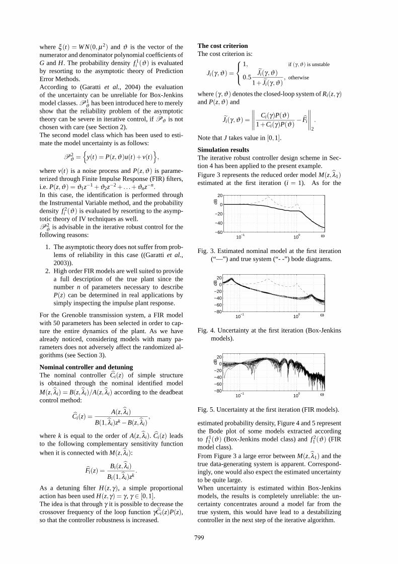
Simulation resultsThe iterative robust controller design scheme in Sec-tion 4 has been applied to the present example.Figure 3 represents the reduced order model M(z, λ1)estimated at the first iteration (i = 1). As for the

10−1

100

−60

−40

−20

0

20

ω

dB

Fig. 3. Estimated nominal model at the first iteration(“—”) and true system (“- -”) bode diagrams.

10−1

100

−80

−60

−40

−20

0

20

ω

dB

Fig. 4. Uncertainty at the first iteration (Box-Jenkinsmodels).

10−1

100

−80

−60

−40

−20

0

20

ω

dB

Fig. 5. Uncertainty at the first iteration (FIR models).

estimated probability density, Figure 4 and 5 representthe Bode plot of some models extracted accordingto f 1

1 (ϑ) (Box-Jenkins model class) and f 21 (ϑ) (FIR

model class).From Figure 3 a large error between M(z, λ1) and thetrue data-generating system is apparent. Correspond-ingly, one would also expect the estimated uncertaintyto be quite large.When uncertainty is estimated within Box-Jenkinsmodels, the results is completely unreliable: the un-certainty concentrates around a model far from thetrue system, this would have lead to a destabilizingcontroller in the next step of the iterative algorithm.

799

When instead FIR models are used, the uncertainty iscorrectly estimated (in fact, it is very scattered aroundthe true system) so that it has been possible to performthe subsequent controller design step. In fact, the ran-domized algorithms have been applied with ε = 0.1and δ = 0.01 while the parameter set of feasible con-trollers Γ = [0,1] has been sampled in p = 30 points.The resulting number q of models extracted accordingto the probability density f 2

1 (ϑ) was 435.The controller obtained at the first iteration is char-acterized by a detuning parameter γ1 equal to 0.06.Its small value indicates a conservative choice whichis justified by the high level of uncertainty. The step-response of the obtained closed-loop system is de-picted in Figure 8.Carrying on the iterative procedure the identified nom-inal model becomes a more and more accurate de-scription of the real plant (Figure 6), and, correspond-

10−1

100

−60

−40

−20

0

20

ω

dB

Fig. 6. Estimated nominal models at iterations i = 2(“—”) and i = 3 (“- -”).

10−1

100

−80

−60

−40

−20

0

20

ω

dB

Fig. 7. Uncertainty at the third iteration (i = 3).

ingly, uncertainty tends to concentrate around the truesystem (see e.g. Figure 7). This leads to the selectionof γ i’s as indicated in Figure 9.As it appears the control performance rapidly im-proves through iterations, preserving always the ro-bust stability (see Figure 8). Figure 10 represents theempirical average cost c(γ i) through iterations.

0 5 10 15 20 25 300

0.2

0.4

0.6

0.8

1

i=3,4

i=2

i=1

Fig. 8. Step response of the closed loop – i = 1, . . . ,4.

6. ACKNOWLEDGEMENTS

Paper supported by the MIUR National ResearchProject “Innovative Techniques for Identification andAdaptive Control of Industrial Systems”, and partiallysupported by CNR-IEIIT

1 2 3 4 50

0.2

0.4

0.6

0.8

1

Fig. 9. γ i at each iteration.

1 2 3 4 50

0.05

0.1

0.15

0.2

0.25

Fig. 10. c(γ i) plotted for each iterations.

REFERENCES

Anderson, B.D.O., X. Bombois, M. Gevers and C. Kulcsàr (1998).Caution in iterative modeling and control design. IFAC Work-shop on Adaptive Control and Signal Processing (Glasgow,UK), 13–19.

Bitmead, R.R., M.Gevers and A.G. Partanen (1997). Introducingcaution in iterative controller design. 11th IFAC Symposiumon System Identification (Fukuoka, Japan), 1701–1706.

Bittanti, S., M.C. Campi and S. Garatti (2002). An iterative con-troller design scheme based on average robust control. 15thWorld IFAC Congress (Barcelona, Spain).

Campi, M.C. and M. Prandini (2003). Randomized algorithms forthe synthesis of cautious adaptive controllers. Systems &Control Letters 49, 21–36.

De Callafon, R.A. and P.M.J. Van den Hof (1997). Suboptimalfeedback control by a scheme of iterative identification andcontrol design. Mathematical Modelling of System 3, 77–101.

Garatti, S., M.C. Campi and S. Bittanti (2003). On the assessment ofthe model quality through the asymptotic theory for an instru-mental variable setting. 42nd IEEE Conference on Decisionand Control (Hawaii, USA), 6015-6020.

Garatti, S., M.C. Campi and S. Bittanti (2004). Assessing the qualityof identified models trough the asymptotic theory - when isthe result reliable? Automatica – to appear (August 2004).

Gevers, M. (2000). A decade of progress in iterative control design:from theory to practice. IFAC Symposium on Advanced Con-trol of Chemical Processes (Pisa, Italy), 677–694.

Landau, I.D., D. Rey, A. Karimi, A. Voda and A. Franco (1995). Aflexible transmission system as a benchmark for robust digitalcontrol. European Journal of Control - special issue.

Lee, W.S., B.D.O. Anderson, I.M.Y. Mareels and R.L. Kosut (1995).On some key issues in the windsurfer approach to adaptiverobust control. Automatica 31, 1619–1636.

Ljung, L. (1999). System Identification: Theory for the User.Prentice-Hall. Upper Saddle River, NJ.

Van den Hof, P.M.J. and R.J.P. Schrama (1995). Identification andcontrol - closed-loop issues. Automatica 31, 1751–1770.

Vidyasagar, M. (2001). Randomized algorithms for robust con-

troller synthesis using statistical learning theory. Automatica

37, 1515–1528.

800