solving systems of linear equations on the cell processor using cholesky factorization

Solving Systems of Linear Equations on theCELL Processor Using Cholesky Factorization

Jakub Kurzak, Member, IEEE, Alfredo Buttari, and Jack Dongarra, Fellow, IEEE

Abstract—The Sony/Toshiba/IBM (STI) CELL processor introduces pioneering solutions in processor architecture. At the same time,

it presents new challenges for the development of numerical algorithms. One is the effective exploitation of the differential between the

speed of single- and double-precision arithmetic; the other is the efficient parallelization between the short-vector Single-Instruction,

Multiple-Data (SIMD) cores. The first challenge is addressed by utilizing the well-known technique of iterative refinement for the

solution of a dense symmetric positive definite system of linear equations, resulting in a mixed-precision algorithm, which delivers

double-precision accuracy while performing the bulk of the work in single precision. The main contribution of this paper lies in

addressing the second challenge by successful thread-level parallelization, exploiting fine-grained task granularity and a lightweight

decentralized synchronization. The implementation of the computationally intensive sections gets within 90 percent of the peak

floating-point performance, while the implementation of the memory-intensive sections reaches within 90 percent of the peak memory

bandwidth. On a single CELL processor, the algorithm achieves more than 170 Gflops when solving a symmetric positive definite

system of linear equations in single precision and more than 150 Gflops when delivering the result in double-precision accuracy.

Index Terms—Parallel algorithms, numerical linear algebra, CELL broadband engine.

Ç

1 MOTIVATION

IN numerical computing, there is a fundamental perfor-mance advantage in using the single-precision floating-

point data format over the double-precision data format,due to the more compact representation, thanks to whichtwice the number of single-precision data elements can bestored at each stage of the memory hierarchy. Short-vectorSingle-Instruction, Multiple-Data (SIMD) processing pro-vides yet more potential for performance gains from usingsingle-precision arithmetic over double precision. Since thegoal is to process the entire vector in a single operation, thecomputation throughput can be doubled when the datarepresentation is halved. Unfortunately, the accuracy of thesolution is also halved.

Most of the processor architectures available today have

been at some point augmented with short-vector SIMD

extensions. Examples include

. Streaming SIMD Extensions (SSE) for the AMD andIntel lines of processors,

. PowerPC Velocity Engine/AltiVec/VMX,

. Sparc Visual Instruction Set (VIS),

. Alpha Motion Video Instructions (MVI),

. PA-RISC Multimedia Acceleration eXtensions (MAX),

. MIPS-3D Application Specific Extensions (ASP) andDigital Media Extensions (MDMX), and

. ARM NEON.

The different architectures exhibit big differences in theircapabilities. The vector size is either 64 bits or, morecommonly, 128 bits. The register file size ranges from just afew to as many as 128 registers. Some extensions onlysupport integer types, others also operate on single-precision floating-point numbers, and yet others alsoprocess double-precision values.

Today, the Synergistic Processing Element (SPE) of theSony/Toshiba/IBM (STI) CELL processor [1], [2], [3] canprobably be considered the state of the art in short-vectorSIMD processing. Possessing 128-byte-long registers and afully pipelined, fused add-multiply instruction, it iscapable of completing eight single-precision floating-pointoperations each clock cycle, which, combined with the sizeof the register file of 128 registers, delivers close-to-peakperformance on many common workloads. At the sametime, built with multimedia and embedded applications inmind, the current incarnation of the CELL architecturedoes not implement double-precision arithmetic on parwith single-precision performance, which makes theprocessor a very attractive target for exploring mixed-precision approaches.

Another important phenomenon in recent years hasbeen the gradual shift of focus in processor architecturefrom aggressive exploitation of instruction-level parallelismtoward thread-level parallelism, resulting in the introduc-tion of chips with multiple processing units commonlyreferred to as multicore processors. The new architecturesdeliver the much desired improvement in performanceand, at the same time, challenge the scalability of existingalgorithms and force the programmers to seek moreparallelism by going to much finer levels of problemgranularity. In linear algebra, it enforces the departurefrom the model relying on parallelism encapsulated at thelevel of BLAS and shifts to more flexible methods ofscheduling work.

IEEE TRANSACTIONS ON PARALLEL AND DISTRIBUTED SYSTEMS, VOL. 19, NO. 9, SEPTEMBER 2008 1175

. The authors are with the Department of Electrical Engineering andComputer Science, University of Tennessee, 1122 Volunteer Blvd Ste413 Claxton, Knoxville, TN 37996-3450.E-mail: {kurzak, buttari, dongarra}@cs.utk.edu.

Manuscript received 10 May 2007; revised 23 Oct. 2007; accepted 8 Nov.2007; published online 28 Nov. 2007.Recommended for acceptance by T. Davis.For information on obtaining reprints of this article, please send e-mail to:[email protected], and reference IEEECS Log Number TPDS-2007-05-0150.Digital Object Identifier no. 10.1109/TPDS.2007.70813.

1045-9219/08/$25.00 � 2008 IEEE Published by the IEEE Computer Society

Authorized licensed use limited to: IEEE Xplore. Downloaded on April 21, 2009 at 15:20 from IEEE Xplore. Restrictions apply.

2 RELATED WORK

Iterative refinement is a well-known method for improvingthe solution of a linear system of equations of the formAx ¼ b. Typically, a dense system of linear equations issolved by applying a factorization to the coefficient matrix,followed by a back solve. Due to round-off errors, thesolution carries an error related to the condition number ofthe coefficient matrix. In order to improve the computedsolution, an iterative refinement process can be applied,which produces a correction to the computed solution ateach iteration. In principle, the algorithm can produce asolution correct to the working precision.

Iterative refinement is a fairly well-understood conceptand was analyzed by Wilkinson [4], Moler [5], and Stewart[6]. Higham gives error bounds for both single- and double-precision iterative refinement algorithms, where the entirealgorithm is implemented with the same precision (single ordouble, respectively) [7]. He also gives error bounds insingle-precision arithmetic, with refinement performed indouble-precision arithmetic. An error analysis for the casedescribed in this work, where the factorization is performedin single precision and the refinement in double precision, isgiven by Langou et al. [8].

The authors of this work have previously presented aninitial implementation of the mixed-precision algorithm forthe general nonsymmetric case using LU factorization on theCELL processors. Although respectable performance num-bers were presented, both the factorization and the refine-ment steps relied on rather classic parallelization approaches.Also, a somewhat general discussion of algorithmic andimplementation details was presented. This work extends theprevious presentation by introducing a novel scheme for theparallelization of the computational components of thealgorithm and also describes in much more detail theimplementation of both computationally intensive andmemory-intensive operations.

Although the thread-level parallelization of the Choleskyfactorizations presented here is quite unique, due to theunique nature of the CELL processor, many of the conceptsare not new. Seminal work in the area of parallel densematrix factorizations was done by Agarwal and Gustavson[9], [10].

3 ALGORITHM

The standard approach to solving symmetric positivedefinite systems of linear equations is to use theCholesky factorization. The Cholesky factorization of areal symmetric positive definite matrix A has the formA ¼ LLT , where L is a real lower triangular matrix withpositive diagonal elements. The system is solved byfirst solving Ly ¼ b (forward substitution) and then solvingLTx ¼ y (backward substitution). In order to improve theaccuracy of the computed solution, an iterative refinementprocess is applied, which produces a correction to thecomputed solution, x.

The mixed-precision iterative refinement algorithmusing Cholesky factorization is outlined in Algorithm 1.The factorization A ¼ LLT (line 2) and the solution of thetriangular systems Ly ¼ b and LTx ¼ y (lines 3 and 8) are

computed using single-precision arithmetic. The residualcalculation (line 6) and the update of the solution (line 10)are computed using double-precision arithmetic and theoriginal double-precision coefficients. The most computa-tionally expensive operations, including the factorization ofthe coefficient matrix A and the forward and backwardsubstitution, are performed using single-precision arith-metic, and they take advantage of the single-precisionspeed. The only operations executed in double precision arethe residual calculation and the update of the solution.

Algorithm 1. Solution of a symmetric positive definite

system of linear equations using mixed-precision iterativerefinement based on Cholesky factorization.

1: Að32Þ, bð32Þ A, b

2: Lð32Þ, LTð32Þ SPOTRFaðAð32ÞÞ

3: xð1Þð32Þ SPOTRSb Lð32Þ; L

Tð32Þ; bð32Þ

� �

4: xð1Þ xð1Þð32Þ

5: repeat

6: rðiÞ b�AxðiÞ7: r

ðiÞð32Þ rðiÞ

8: zðiÞð32Þ SPOTRSb Lð32Þ; L

Tð32Þ; r

ðiÞð32Þ

� �

9: zðiÞ zðiÞð32Þ

10: xðiþ1Þ xðiÞ þ zðiÞ11: until xðiÞ is accurate enough

aLAPACK name for Cholesky factorizationbLAPACK name for symmetric forward/backward

substitution

A 64-bit representation is used in all cases where a 32-bit

representation is not indicated by a subscript.

It can be observed that all operations of Oðn3Þ complexityare handled in single precision, and all operations per-formed in double precision are of at most Oðn2Þ complexity.The coefficient matrix A is converted to single precision forthe Cholesky factorization. At the same time, the originalmatrix in double precision is preserved for the residualcalculation.

The algorithm described above and shown in Algorithm 1is available in the LAPACK 3.1 library and implemented bythe routine DSGESV.

4 IMPLEMENTATION

4.1 Essential Hardware Features

An extensive hardware overview would be beyond thescope of this publication. Vast amounts of information arepublicly available for both experienced programmers [11]and newcomers to the field [12], [13]. It is assumed that thereader has some familiarity with the architecture. Here, thefeatures that have the most influence on the implementationpresented are mentioned.

The CELL is a multicore chip that includes nine differentprocessing elements. One core, the POWER Processing Ele-ment (PPE), represents a standard processor design imple-menting the PowerPC instruction set. The remaining eightcores, the SPEs, are short-vector SIMD engines with bigregister files of 128 128-bit vector registers and 256 Kbytes oflocal memory, referred to as local store (LS).

1176 IEEE TRANSACTIONS ON PARALLEL AND DISTRIBUTED SYSTEMS, VOL. 19, NO. 9, SEPTEMBER 2008


Although standard C code can be compiled for theexecution on the SPEs, the SPEs do not execute scalar codeefficiently. For efficient execution, the code has to bevectorized in the SIMD sense, by using C language vectorextensions (intrinsics) or by using assembly code. Thesystem’s main memory is accessible to the PPE through L1and L2 caches and to the SPEs through DMA enginesassociated with them. The SPEs can only execute the coderesiding in the LS and can only operate on the data in theLS. All data has to be transferred in and out of LS viaDMA transfers.

The theoretical computing power of a single SPE is25.6 Gflops in single precision and roughly 1.8 Gflops indouble precision. The floating-point arithmetic follows theIEEE format, with double-precision operations complyingnumerically with the standard and single precision provid-ing only rounding toward zero. The theoretical commu-nication speed for a single SPE is 25.6 Gbytes/s. Thetheoretical peak bandwidth of the main memory is25.6 Gbytes/s as well (shared by the PPE and all SPEs).

The size of the register file and the size of the LS dictatethe size of the elementary operation subject to scheduling tothe SPEs. The ratio of computing power to the memorybandwidth dictates the overall problem decomposition forparallel execution.

4.2 Factorization

A few varieties of Cholesky factorization are known, inparticular the right-looking variant and the left-lookingvariant [14]. It has also been pointed out that those variantsare borders of a continuous spectrum of possible executionpaths [15].

Generally, the left-looking factorization is preferred forseveral reasons. During the factorization, most time is spentcalculating a matrix-matrix product. In the case of the right-looking factorization, this product involves a triangularmatrix. In the case of the left-looking factorization, thisproduct only involves rectangular matrices. It is generallymore efficient to implement a matrix-matrix product forrectangular matrices, and it is easier to balance the load inparallel execution. The implementation presented here is

derived from the left-looking formulation of the Choleskyfactorization, which follows the implementation of theLAPACK routine SPOTRF.

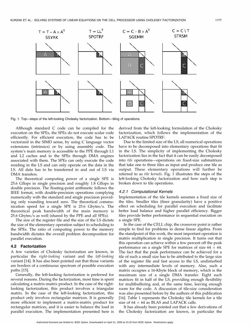
Due to the limited size of the LS, all numerical operationshave to be decomposed into elementary operations that fitin the LS. The simplicity of implementing the Choleskyfactorization lies in the fact that it can be easily decomposedinto tile operations—operations on fixed-size submatricesthat take one to three tiles as input and produce one tile asoutput. These elementary operations will further bereferred to as tile kernels. Fig. 1 illustrates the steps of theleft-looking Cholesky factorization and how each step isbroken down to tile operations.

4.2.1 Computational Kernels

Implementation of the tile kernels assumes a fixed size ofthe tiles. Smaller tiles (finer granularity) have a positiveeffect on scheduling for parallel execution and facilitatebetter load balance and higher parallel efficiency. Biggertiles provide better performance in sequential execution ona single SPE.

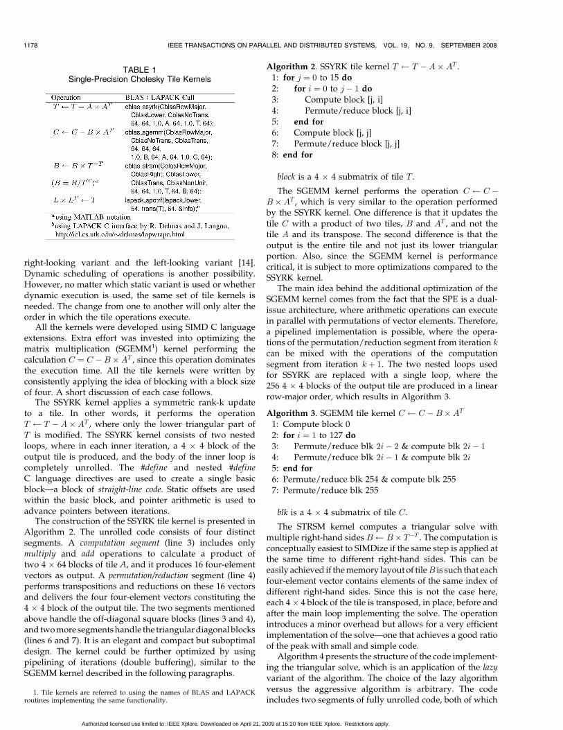
In the case of the CELL chip, the crossover point is rathersimple to find for problems in dense linear algebra. Fromthe standpoint of this work, the most important operation ismatrix multiplication in single precision. It turns out thatthis operation can achieve within a few percent off the peakperformance on a single SPE for matrices of size 64 � 64.The fact that the peak performance can be achieved for atile of such a small size has to be attributed to the large sizeof the register file and fast access to the LS, undisturbedwith any intermediate levels of memory. Also, such amatrix occupies a 16-Kbyte block of memory, which is themaximum size of a single DMA transfer. Eight suchmatrices fit in half of the LS, providing enough flexibilityfor multibuffering and, at the same time, leaving enoughroom for the code. A discussion of tile-size considerationwas also presented before by the authors of this publication[16]. Table 1 represents the Cholesky tile kernels for a tilesize of 64 � 64 as BLAS and LAPACK calls.

It has already been pointed out that a few derivations ofthe Cholesky factorization are known, in particular the

KURZAK ET AL.: SOLVING SYSTEMS OF LINEAR EQUATIONS ON THE CELL PROCESSOR USING CHOLESKY FACTORIZATION 1177

Fig. 1. Top—steps of the left-looking Cholesky factorization. Bottom—tiling of operations.


right-looking variant and the left-looking variant [14].Dynamic scheduling of operations is another possibility.However, no matter which static variant is used or whetherdynamic execution is used, the same set of tile kernels isneeded. The change from one to another will only alter theorder in which the tile operations execute.

All the kernels were developed using SIMD C languageextensions. Extra effort was invested into optimizing thematrix multiplication (SGEMM1) kernel performing thecalculation C ¼ C �B�AT , since this operation dominatesthe execution time. All the tile kernels were written byconsistently applying the idea of blocking with a block sizeof four. A short discussion of each case follows.

The SSYRK kernel applies a symmetric rank-k updateto a tile. In other words, it performs the operationT T �A�AT , where only the lower triangular part ofT is modified. The SSYRK kernel consists of two nestedloops, where in each inner iteration, a 4 � 4 block of theoutput tile is produced, and the body of the inner loop iscompletely unrolled. The #define and nested #defineC language directives are used to create a single basicblock—a block of straight-line code. Static offsets are usedwithin the basic block, and pointer arithmetic is used toadvance pointers between iterations.

The construction of the SSYRK tile kernel is presented inAlgorithm 2. The unrolled code consists of four distinctsegments. A computation segment (line 3) includes onlymultiply and add operations to calculate a product oftwo 4 � 64 blocks of tile A, and it produces 16 four-elementvectors as output. A permutation/reduction segment (line 4)performs transpositions and reductions on these 16 vectorsand delivers the four four-element vectors constituting the4 � 4 block of the output tile. The two segments mentionedabove handle the off-diagonal square blocks (lines 3 and 4),and two more segments handle the triangular diagonal blocks(lines 6 and 7). It is an elegant and compact but suboptimaldesign. The kernel could be further optimized by usingpipelining of iterations (double buffering), similar to theSGEMM kernel described in the following paragraphs.

Algorithm 2. SSYRK tile kernel T T �A�AT .1: for j ¼ 0 to 15 do

2: for i ¼ 0 to j� 1 do

3: Compute block [j, i]

4: Permute/reduce block [j, i]

5: end for

6: Compute block [j, j]

7: Permute/reduce block [j, j]

8: end for

block is a 4 � 4 submatrix of tile T .

The SGEMM kernel performs the operation C C �B�AT , which is very similar to the operation performedby the SSYRK kernel. One difference is that it updates thetile C with a product of two tiles, B and AT , and not thetile A and its transpose. The second difference is that theoutput is the entire tile and not just its lower triangularportion. Also, since the SGEMM kernel is performancecritical, it is subject to more optimizations compared to theSSYRK kernel.

The main idea behind the additional optimization of theSGEMM kernel comes from the fact that the SPE is a dual-issue architecture, where arithmetic operations can executein parallel with permutations of vector elements. Therefore,a pipelined implementation is possible, where the opera-tions of the permutation/reduction segment from iteration kcan be mixed with the operations of the computationsegment from iteration kþ 1. The two nested loops usedfor SSYRK are replaced with a single loop, where the256 4 � 4 blocks of the output tile are produced in a linearrow-major order, which results in Algorithm 3.

Algorithm 3. SGEMM tile kernel C C �B�AT

1: Compute block 0

2: for i ¼ 1 to 127 do

3: Permute/reduce blk 2i� 2 & compute blk 2i� 1

4: Permute/reduce blk 2i� 1 & compute blk 2i

5: end for

6: Permute/reduce blk 254 & compute blk 255

7: Permute/reduce blk 255

blk is a 4 � 4 submatrix of tile C.

The STRSM kernel computes a triangular solve withmultiple right-hand sides B B� T�T . The computation isconceptually easiest to SIMDize if the same step is applied atthe same time to different right-hand sides. This can beeasily achieved if the memory layout of tileB is such that eachfour-element vector contains elements of the same index ofdifferent right-hand sides. Since this is not the case here,each 4� 4 block of the tile is transposed, in place, before andafter the main loop implementing the solve. The operationintroduces a minor overhead but allows for a very efficientimplementation of the solve—one that achieves a good ratioof the peak with small and simple code.

Algorithm 4 presents the structure of the code implement-ing the triangular solve, which is an application of the lazyvariant of the algorithm. The choice of the lazy algorithmversus the aggressive algorithm is arbitrary. The codeincludes two segments of fully unrolled code, both of which


TABLE 1Single-Precision Cholesky Tile Kernels

1. Tile kernels are referred to using the names of BLAS and LAPACKroutines implementing the same functionality.


operate on 64 � 4 blocks of data. The outer loop segment

(line 5) produces a 64 � 4 block j of the solution. The inner

loop segment (line 3) applies the update of step i to block j.

Algorithm 4. STRSM tile kernel B B� T�T .1: for j ¼ 0 to 15 do

2: for i ¼ 0 to j� 1 do

3: Apply block i toward block j

4: end for

5: Solve block j

6: end for

block is a 64 � 4 submatrix of tile B.

The SPOTRF kernel computes the Cholesky factorization,T L� LT , of a 64 � 64 tile. This is the lazy variant of thealgorithm, more commonly referred to as the left-lookingfactorization, where updates to the trailing submatrix do notimmediately follow panel factorization. Instead, updatesare applied to a panel right before the factorization ofthat panel.

It could be expected that this kernel is implemented usingLevel-2 BLAS operations, as this is the usual way ofimplementing panel factorizations. Such a solution would,however, lead to the code being difficult to SIMDize andyield very poor performance. Instead, the implementation ofthis routine is simply an application of the idea of blockingwith a block size equal to the SIMD vector size of four.Algorithm 5 presents the structure of the SPOTRF tile kernel.

Algorithm 5. SPOTRF tile kernel T L� LT .

1: for k ¼ 0 to 15 do

2: for i ¼ 0 to k� 1 do

3: SSYRK (apply block [k, i] to block [k, k])4: end for

5: SPOTF2 (factorize block [k, k])

6: for j ¼ k to 15 do

7: for i ¼ 0 to k� 1 do

8: SGEMM (apply block [j, i] to block [j, k])

9: end for

10: end for

11: for j ¼ k to 15 do

12: STRSM (apply block [k, k] to block [j, k])

13: end for

14: end for

block is a 4 � 4 submatrix of tile T .

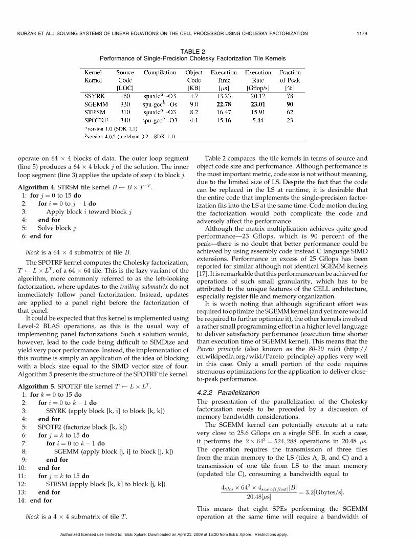
Table 2 compares the tile kernels in terms of source andobject code size and performance. Although performance isthe most important metric, code size is not without meaning,due to the limited size of LS. Despite the fact that the codecan be replaced in the LS at runtime, it is desirable thatthe entire code that implements the single-precision factor-ization fits into the LS at the same time. Code motion duringthe factorization would both complicate the code andadversely affect the performance.

Although the matrix multiplication achieves quite goodperformance—23 Gflops, which is 90 percent of thepeak—there is no doubt that better performance could beachieved by using assembly code instead C language SIMDextensions. Performance in excess of 25 Gflops has beenreported for similar although not identical SGEMM kernels[17]. It is remarkable that this performance can be achieved foroperations of such small granularity, which has to beattributed to the unique features of the CELL architecture,especially register file and memory organization.

It is worth noting that although significant effort wasrequired to optimize the SGEMM kernel (and yet more wouldbe required to further optimize it), the other kernels involveda rather small programming effort in a higher level languageto deliver satisfactory performance (execution time shorterthan execution time of SGEMM kernel). This means that thePareto principle (also known as the 80-20 rule) (http://en.wikipedia.org/wiki/Pareto_principle) applies very wellin this case. Only a small portion of the code requiresstrenuous optimizations for the application to deliver close-to-peak performance.

4.2.2 Parallelization

The presentation of the parallelization of the Choleskyfactorization needs to be preceded by a discussion ofmemory bandwidth considerations.

The SGEMM kernel can potentially execute at a rate

very close to 25.6 Gflops on a single SPE. In such a case,

it performs the 2� 643 ¼ 524; 288 operations in 20.48 �s.

The operation requires the transmission of three tiles

from the main memory to the LS (tiles A, B, and C) and a

transmission of one tile from LS to the main memory

(updated tile C), consuming a bandwidth equal to

4tiles � 642 � 4size ofðfloatÞ½B�20:48½�s� ¼ 3:2½Gbytes=s�:

This means that eight SPEs performing the SGEMMoperation at the same time will require a bandwidth of


TABLE 2Performance of Single-Precision Cholesky Factorization Tile Kernels


8� 3:2 Gbytes=s ¼ 25:6 Gbytes=s, which is the theoreticalpeak main memory bandwidth.

It has been shown that arithmetic can execute almost at thetheoretical peak rate on the SPE. At the same time, it wouldnot be realistic to expect the theoretical peak bandwidthfrom the memory system. By the same token, data reuse hasto be introduced into the algorithm to decrease the load onthe main memory. A straightforward solution is to introduce1D processing, where each SPE processes one row of tiles ofthe coefficient matrix at a time.

Please see Fig. 1 for the following discussion. In theSSYRK part, one SPE applies a row of tiles A to the diagonaltile T , followed by the SPOTRF operation (factorization) ofthe tile T . Tile T only needs to be read in at the beginning ofthis step and written back at the end. The only transferstaking place in between are reads of tiles A. Similarly, in theSGEMM part, one SPE applies a row of tiles A and a row oftiles B to tile C, followed by the STRSM operation(triangular solve) on tile C using the diagonal triangulartile T . Tile C only needs to be read in at the beginning of thisstep and written back at the end. Tile T only needs to beread in right before the triangular solve. The only transferstaking place in between are reads of tiles A and B. Suchwork partitioning approximately halves the load on thememory system.

It may also be noted that 1D processing is a naturalmatch for the left-looking factorization. In the right-lookingfactorization, the update to the trailing submatrix can easilybe partitioned in two dimensions. However, in the case ofthe left-looking factorization, 2D partitioning would not befeasible due to the write dependency on the panel blocks(tiles T and C).

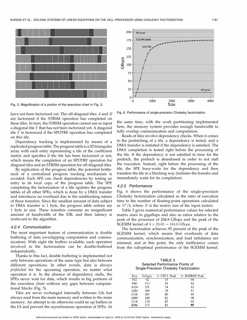
One-dimensional partitioning introduces a load balan-cing problem. With work being distributed by block rows,in each step of the factorization, a number of processors aregoing to be idle, which are equal to the number of block

rows factorized in a particular step modulo the number ofprocessors. Fig. 3 shows three consecutive steps on afactorization with the processors being occupied and idle inthese steps. Such behavior is going to put a harsh upperbound on achievable performance.

It can be observed, however, that at each step of thefactorization, a substantial amount of work can be sched-uled, to the otherwise idle processors, from the upcomingsteps of the factorization. The only operations that cannot bescheduled at a given point in time are those that involvepanels that have not been factorized yet. This situation isillustrated in Fig. 4. Of course, this kind of processingrequires dependency tracking in two dimensions, but sinceall operations proceed at the granularity of tiles, this doesnot pose a problem.

In the implementation presented here, all SPEs follow astatic schedule, presented in Fig. 4, with cyclic distributionof work from the steps of the factorization. In this case, astatic schedule works well, due to the fact that theperformance of the SPEs is very deterministic (unaffectedby any nondeterministic phenomena like cache misses).This way, the potential bottleneck of a centralized schedul-ing mechanism is avoided.

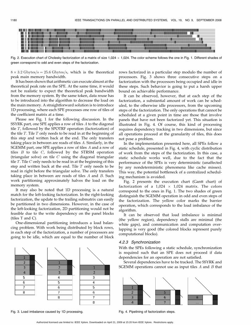
Fig. 2 presents the execution chart (Gantt chart) offactorization of a 1,024 � 1,024 matrix. The colorscorrespond to the ones in Fig. 1. The two shades of greendistinguish the SGEMM operation in odd and even steps ofthe factorization. The yellow color marks the barrieroperation, which corresponds to the load imbalance of thealgorithm.

It can be observed that load imbalance is minimal(the yellow region), dependency stalls are minimal (thewhite gaps), and communication and computation over-lapping is very good (the colored blocks represent purelycomputational blocks).

4.2.3 Synchronization

With the SPEs following a static schedule, synchronizationis required such that an SPE does not proceed if datadependencies for an operation are not satisfied.

Several dependencies have to be tracked. The SSYRK andSGEMM operations cannot use as input tiles A and B that


Fig. 2. Execution chart of Cholesky factorization of a matrix of size 1,024 � 1,024. The color scheme follows the one in Fig. 1. Different shades of

green correspond to odd and even steps of the factorization.

Fig. 3. Load imbalance caused by 1D processing. Fig. 4. Pipelining of factorization steps.


have not been factorized yet. The off-diagonal tiles A and Bare factorized if the STRSM operation has completed onthese tiles. In turn, the STRSM operation cannot use as inputa diagonal tile T that has not been factorized yet. A diagonaltile T is factorized if the SPOTRF operation has completedon this tile.

Dependency tracking is implemented by means of areplicated progress table. The progress table is a 2D triangulararray with each entry representing a tile of the coefficientmatrix and specifies if the tile has been factorized or not,which means the completion of an SPOTRF operation fordiagonal tiles and an STRSM operation for off-diagonal tiles.

By replication of the progress table, the potential bottle-neck of a centralized progress tracking mechanism isavoided. Each SPE can check dependencies by testing anentry in its local copy of the progress table. The SPEcompleting the factorization of a tile updates the progresstables of all other SPEs, which is done by a DMA transferand introduces no overhead due to the nonblocking natureof these transfers. Since the smallest amount of data subjectto DMA transfer is 1 byte, the progress table entries are1 byte in size. These transfers consume an insignificantamount of bandwidth of the EIB, and their latency isirrelevant to the algorithm.

4.2.4 Communication

The most important feature of communication is doublebuffering of data (overlapping computation and commu-nication). With eight tile buffers available, each operationinvolved in the factorization can be double-bufferedindependently.

Thanks to this fact, double buffering is implemented notonly between operations of the same type but also betweendifferent operations. In other words, data is alwaysprefetched for the upcoming operation, no matter whatoperation it is. In the absence of dependency stalls, theSPEs never wait for data, which results in big portions ofthe execution chart without any gaps between computa-tional blocks (Fig. 5).

Tiles are never exchanged internally between LSs butalways read from the main memory and written to the mainmemory. An attempt to do otherwise could tie up buffers inthe LS and prevent the asynchronous operation of SPEs. At

the same time, with the work partitioning implementedhere, the memory system provides enough bandwidth tofully overlap communication and computation.

Reads of tiles involve dependency checks. When it comesto the prefetching of a tile, a dependency is tested, and aDMA transfer is initiated if the dependency is satisfied. TheDMA completion is tested right before the processing ofthe tile. If the dependency is not satisfied in time for theprefetch, the prefetch is abandoned in order to not stallthe execution. Instead, right before the processing of thetile, the SPE busy-waits for the dependency and thentransfers the tile in a blocking way (initiates the transfer andimmediately waits for its completion).

4.2.5 Performance

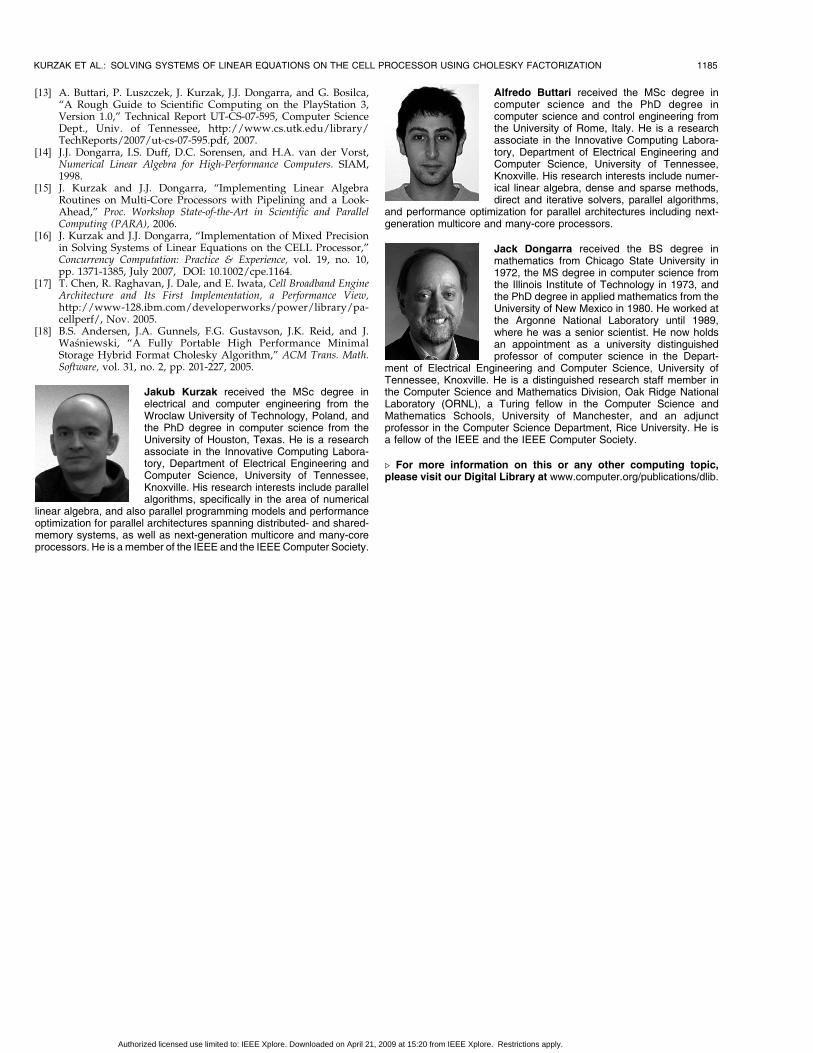
Fig. 6 shows the performance of the single-precisionCholesky factorization calculated as the ratio of executiontime to the number of floating-point operations calculatedas N3=3, where N is the matrix size of the input matrix.

Table 3 gives numerical performance values for selectedmatrix sizes in gigaflops and also as ratios relative to thepeak of the processor of 204.8 Gflops and the peak of theSGEMM kernel of 8� 23:01 ¼ 184:8 Gflops.

The factorization achieves 95 percent of the peak of theSGEMM kernel, which means that overheads of datacommunication, synchronization, and load imbalance areminimal, and at this point, the only inefficiency comesfrom the suboptimal performance of the SGEMM kernel.


Fig. 5. Magnification of a portion of the execution chart in Fig. 2.

Fig. 6. Performance of single-precision Cholesky factorization.

TABLE 3Selected Performance Points of

Single-Precision Cholesky Factorization


Hopefully, in the future, the kernel will be fully optimized,perhaps using hand-coded assembly.

4.3 Refinement

The two most expensive operations of the refinement arethe back solve (Algorithm 1, steps 3 and 8) and residualcalculation (Algorithm 1, step 6).

The back solve consists of two triangular solves invol-ving the entire coefficient matrix and a single right-hand side(BLAS STRSV operation). The residual calculation is adouble-precision matrix-vector product using a symmetricmatrix (BLAS DSYMV operation).

Both operations are BLAS Level-2 operations and, onmost processors, would be strictly memory bound. TheSTRSV operation actually is a perfect example of a strictlymemory-bound operation on the CELL processor. How-ever, the DSYMV operation is on the borderline of beingmemory bound versus computationally bound due to thevery high speed of the memory system versus the relativelylow performance of the double-precision arithmetic.

4.3.1 Triangular Solve

The triangular solve is a perfect example of a memory-bound workload, where the memory access rate sets theupper limit on achievable performance. The STRSV per-forms approximately two floating-point operations per eachdata element of 4 bytes, which means that the peak memorybandwidth of 25.6 Gbytes/s allows for at most

25:6 Gbytes=s� 2ops=float=4bytes=float ¼ 12:8 Gflop=s;

which is only 1/16 or 0.625 percent of the single-precisionfloating-point peak of the processor. Owing to this fact, thegoal of implementing memory-bound operations is to getclose to the peak memory bandwidth, unlike for computa-tionally bound operations, where the goal is to get close tothe floating-point peak. This task should be readilyachievable, given that a single SPE possesses as muchbandwidth as the main memory.

Practice shows, however, that a single SPE is not capableof generating enough traffic to fully exploit the bandwidth,and a few SPEs solving the problem in parallel should beused. Efficient parallel implementation of the STRSVoperation has to pursue two goals: continuous generationof traffic in order to saturate the memory system andaggressive pursuit of the algorithmic critical path in orderto avoid dependency stalls. A related question is the desiredlevel of parallelism—the optimal number of processing

elements used. Since the triangular solve is rich independencies, increasing the number of SPEs increasesthe number of execution stalls caused by interprocessordependencies. Obviously, there is a crossover point, a sweetspot, for the number of SPEs used for the operation.

Same as other routines in the code, the STRSV operationprocesses the coefficient matrix by 64 � 64 tiles. Triangularsolve is performed on the diagonal tiles, and a matrix-vectorproduct (SGEMV equivalent) is performed on the off-diagonal tiles. Processing of the diagonal tiles constitutesthe critical path in the algorithm. One SPE is solely devoted tothe processing of the diagonal tiles, while the goal of theothers is to saturate the memory system with processing ofthe off-diagonal tiles. The number of SPEs used to process theoff-diagonal tiles is a function of a few parameters. Theefficiency of the computational kernels used is one of thefactors. In this case, the number four turned out to deliver thebest results, with one SPE pursuing the critical path and threeothers fulfilling the task of memory saturation. Fig. 7 presentsthe distribution of work in the triangular solve routines.

The solve is done in place. The unknown/solution vectoris read in its entirety by each SPE to its LS at the beginningand returned to the main memory at the end. As thecomputation proceeds, updated pieces of the vector areexchanged internally by means of direct LS-to-LS commu-nication. At the end, SPE 0 possesses the full solution vectorand writes it back to the main memory. Synchronization isimplemented analogously to the synchronization in thefactorization and is based on the replicated triangularprogress table (the same data structure is reused).

Fig. 8 shows the performance, in terms of gigabytes persecond, of the two triangular solve routines required in thesolution/refinement step of the algorithm. The two routinesperform slightly differently due to the different perfor-mance of their computational kernels. The figure showsclearly that the goal of saturating the memory system isachieved quite well. Performance as high as 23.77 Gbytes/sis obtained, which is 93 percent of the peak.

4.3.2 Matrix-Vector Product

For most hardware platforms the matrix-vector productwould be a memory-bound operation, the same as the


Fig. 7. Distribution of work in the triangular solve routine.

Fig. 8. Performance of the triangular solve routines.


triangular solve. On the CELL processor, however, due tothe relative slowness of the double-precision arithmetic, theoperation is on the border of being memory bound andcomputationally bound. Even with the use of all eight SPEs,saturation of the memory is harder than in the case of theSTRSV routine.

The DSYMV routine also operates on tiles. Here,however, the double-precision representation of the coeffi-cient matrix is used with a tile size of 32 � 32 such that anentire tile can also be transferred with a single DMArequest. The input vector is only read in once, at thebeginning, in its entirety, and the output vector is writtenback after the computation is completed. Since the inputmatrix is symmetric, only the lower portion is accessed, andimplicit transposition is used to reflect the effect of theupper portion—each tile is read in only once but applied tothe output vector twice (with and without transposition).

Since load balance is a very important aspect of theimplementation, work is split among SPEs very evenly byapplying the partitioning reflected in Fig. 9. Such workdistribution causes multiple write dependencies on theoutput vector, and in order to let each SPE proceed withoutstalls, the output vector is replicated on each SPE, and themultiplication is followed by a reduction step. Thereduction is also performed in parallel by all SPEs andintroduces a very small overhead, compensated by thebenefits of very good load balance.

Fig. 10 shows the performance, in terms of gigabytes persecond, of the double-precision symmetric matrix-vectorproduct routine. A performance of 20.93 Gbytes/s isachieved, which is 82 percent of the peak. Although theDSYMV routine represents a Level-2 BLAS operation and isparallelized among all SPEs, it is still computationallybound. Perhaps, its computational components could befurther optimized. Nevertheless, at this point, the deliveredlevel of performance is considered satisfactory.

5 LIMITATIONS

The implementation presented here should be considered aproof-of-concept prototype with the purpose of establishingan upper bound on the performance achievable for mixed-precision dense linear algebra algorithms on the CELLprocessor. As such, it has a number of limitations. Onlysystems that are multiples of 64 in size are accepted, whichmeans that the cost of solving a system of size 65 � 65 isequal to the cost of solving a system of size 128 � 128. Also,only systems with a single right-hand side are supported.

There are no tests for overflow during conversions fromdouble to single precision. There is no test for the positivedefinite property during the single-precision factorizationstep, so it is up to the user to guarantee this attribute. Themaximum size of the coefficient matrix is set to 4,096,which makes it possible to fit the progress table in each LS.This also makes it possible to fit the entire unknown/solution vector in each LS, which facilitates internal LS-to-LS communication and is very beneficial for performance.The current implementation is wasteful in its use of themain memory. The entire coefficient matrix is storedexplicitly without taking advantage of its symmetry, inboth single-precision representation and double-precisionrepresentation, an issue that can be resolved by usingspecialized storage formats [18].

6 RESULTS AND DISCUSSION

Fig. 11 compares the performance of a single-precisionfactorization (SPOTRF), the solution of the system in singleprecision (SPOSV), and the solution of the system in doubleprecision by using factorization in single precision anditerative refinement to double precision (DSPOSV). Theseresults were obtained on an IBM CELL blade using one ofthe two available CELL processors. Huge memory pages(16 Mbytes) were used for improved performance [16]. Theperformance is calculated as the ratio of the execution timeto the number of floating-point operations, which is set inall cases to N3=3. In all cases, well-conditioned inputmatrices were used, resulting in two steps of refinementdelivering accuracy equal to or higher than the onedelivered by the purely double-precision algorithm.

At the maximum size of 4,096, the factorization achieves175 Gflops, and the system solution runs at the relative speedof 171 Gflops. At the same time, the solution in doubleprecision using the refinement technique delivers therelative performance of 156 Gflops, which is an overheadof less than 9 percent compared to the solution of the systemin single precision. It can also be pointed outthat by using themixed-precision algorithm, double-precision results aredelivered at a speed more than 10 times greater than thedouble-precision peak of the processor.


Fig. 9. Distribution of work in the matrix-vector product routine.

Fig. 10. Performance of the matrix-vector product routine.


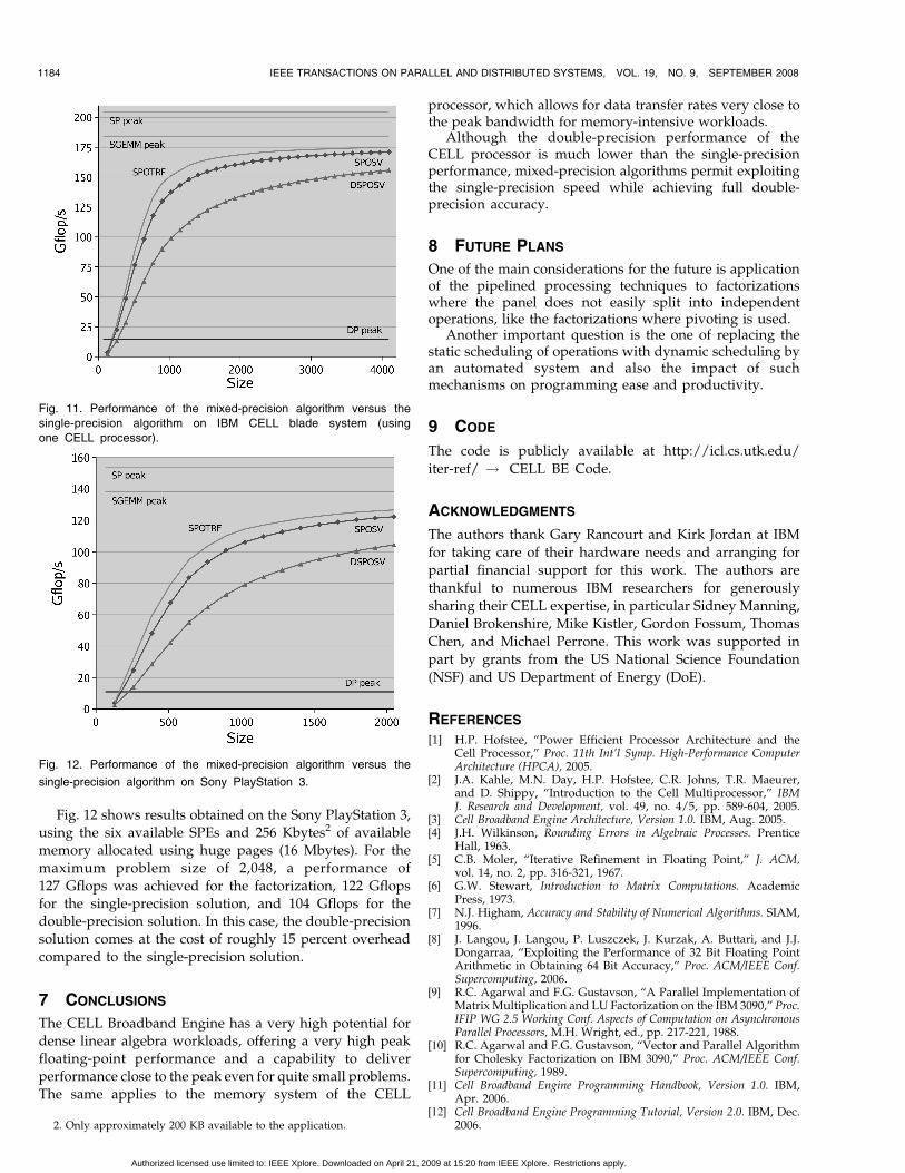
Fig. 12 shows results obtained on the Sony PlayStation 3,

using the six available SPEs and 256 Kbytes2 of available

memory allocated using huge pages (16 Mbytes). For the

maximum problem size of 2,048, a performance of

127 Gflops was achieved for the factorization, 122 Gflops

for the single-precision solution, and 104 Gflops for the

double-precision solution. In this case, the double-precision

solution comes at the cost of roughly 15 percent overhead

compared to the single-precision solution.

7 CONCLUSIONS

The CELL Broadband Engine has a very high potential for

dense linear algebra workloads, offering a very high peak

floating-point performance and a capability to deliver

performance close to the peak even for quite small problems.

The same applies to the memory system of the CELL

processor, which allows for data transfer rates very close tothe peak bandwidth for memory-intensive workloads.

Although the double-precision performance of theCELL processor is much lower than the single-precisionperformance, mixed-precision algorithms permit exploitingthe single-precision speed while achieving full double-precision accuracy.

8 FUTURE PLANS

One of the main considerations for the future is applicationof the pipelined processing techniques to factorizationswhere the panel does not easily split into independentoperations, like the factorizations where pivoting is used.

Another important question is the one of replacing thestatic scheduling of operations with dynamic scheduling byan automated system and also the impact of suchmechanisms on programming ease and productivity.

9 CODE

The code is publicly available at http://icl.cs.utk.edu/

iter-ref/ ! CELL BE Code.

ACKNOWLEDGMENTS

The authors thank Gary Rancourt and Kirk Jordan at IBM

for taking care of their hardware needs and arranging for

partial financial support for this work. The authors are

thankful to numerous IBM researchers for generously

sharing their CELL expertise, in particular Sidney Manning,

Daniel Brokenshire, Mike Kistler, Gordon Fossum, Thomas

Chen, and Michael Perrone. This work was supported in

part by grants from the US National Science Foundation

(NSF) and US Department of Energy (DoE).

REFERENCES

[1] H.P. Hofstee, “Power Efficient Processor Architecture and theCell Processor,” Proc. 11th Int’l Symp. High-Performance ComputerArchitecture (HPCA), 2005.

[2] J.A. Kahle, M.N. Day, H.P. Hofstee, C.R. Johns, T.R. Maeurer,and D. Shippy, “Introduction to the Cell Multiprocessor,” IBMJ. Research and Development, vol. 49, no. 4/5, pp. 589-604, 2005.

[3] Cell Broadband Engine Architecture, Version 1.0. IBM, Aug. 2005.[4] J.H. Wilkinson, Rounding Errors in Algebraic Processes. Prentice

Hall, 1963.[5] C.B. Moler, “Iterative Refinement in Floating Point,” J. ACM,

vol. 14, no. 2, pp. 316-321, 1967.[6] G.W. Stewart, Introduction to Matrix Computations. Academic

Press, 1973.[7] N.J. Higham, Accuracy and Stability of Numerical Algorithms. SIAM,

1996.[8] J. Langou, J. Langou, P. Luszczek, J. Kurzak, A. Buttari, and J.J.

Dongarraa, “Exploiting the Performance of 32 Bit Floating PointArithmetic in Obtaining 64 Bit Accuracy,” Proc. ACM/IEEE Conf.Supercomputing, 2006.

[9] R.C. Agarwal and F.G. Gustavson, “A Parallel Implementation ofMatrix Multiplication and LU Factorization on the IBM 3090,” Proc.IFIP WG 2.5 Working Conf. Aspects of Computation on AsynchronousParallel Processors, M.H. Wright, ed., pp. 217-221, 1988.

[10] R.C. Agarwal and F.G. Gustavson, “Vector and Parallel Algorithmfor Cholesky Factorization on IBM 3090,” Proc. ACM/IEEE Conf.Supercomputing, 1989.

[11] Cell Broadband Engine Programming Handbook, Version 1.0. IBM,Apr. 2006.

[12] Cell Broadband Engine Programming Tutorial, Version 2.0. IBM, Dec.2006.


Fig. 11. Performance of the mixed-precision algorithm versus the

single-precision algorithm on IBM CELL blade system (using

one CELL processor).

2. Only approximately 200 KB available to the application.

Fig. 12. Performance of the mixed-precision algorithm versus the

single-precision algorithm on Sony PlayStation 3.


[13] A. Buttari, P. Luszczek, J. Kurzak, J.J. Dongarra, and G. Bosilca,“A Rough Guide to Scientific Computing on the PlayStation 3,Version 1.0,” Technical Report UT-CS-07-595, Computer ScienceDept., Univ. of Tennessee, http://www.cs.utk.edu/library/TechReports/2007/ut-cs-07-595.pdf, 2007.

[14] J.J. Dongarra, I.S. Duff, D.C. Sorensen, and H.A. van der Vorst,Numerical Linear Algebra for High-Performance Computers. SIAM,1998.

[15] J. Kurzak and J.J. Dongarra, “Implementing Linear AlgebraRoutines on Multi-Core Processors with Pipelining and a Look-Ahead,” Proc. Workshop State-of-the-Art in Scientific and ParallelComputing (PARA), 2006.

[16] J. Kurzak and J.J. Dongarra, “Implementation of Mixed Precisionin Solving Systems of Linear Equations on the CELL Processor,”Concurrency Computation: Practice & Experience, vol. 19, no. 10,pp. 1371-1385, July 2007, DOI: 10.1002/cpe.1164.

[17] T. Chen, R. Raghavan, J. Dale, and E. Iwata, Cell Broadband EngineArchitecture and Its First Implementation, a Performance View,http://www-128.ibm.com/developerworks/power/library/pa-cellperf/, Nov. 2005.

[18] B.S. Andersen, J.A. Gunnels, F.G. Gustavson, J.K. Reid, and J.Wa�sniewski, “A Fully Portable High Performance MinimalStorage Hybrid Format Cholesky Algorithm,” ACM Trans. Math.Software, vol. 31, no. 2, pp. 201-227, 2005.

Jakub Kurzak received the MSc degree inelectrical and computer engineering from theWroclaw University of Technology, Poland, andthe PhD degree in computer science from theUniversity of Houston, Texas. He is a researchassociate in the Innovative Computing Labora-tory, Department of Electrical Engineering andComputer Science, University of Tennessee,Knoxville. His research interests include parallelalgorithms, specifically in the area of numerical

linear algebra, and also parallel programming models and performanceoptimization for parallel architectures spanning distributed- and shared-memory systems, as well as next-generation multicore and many-coreprocessors. He is a member of the IEEE and the IEEE Computer Society.

Alfredo Buttari received the MSc degree incomputer science and the PhD degree incomputer science and control engineering fromthe University of Rome, Italy. He is a researchassociate in the Innovative Computing Labora-tory, Department of Electrical Engineering andComputer Science, University of Tennessee,Knoxville. His research interests include numer-ical linear algebra, dense and sparse methods,direct and iterative solvers, parallel algorithms,

and performance optimization for parallel architectures including next-generation multicore and many-core processors.

Jack Dongarra received the BS degree inmathematics from Chicago State University in1972, the MS degree in computer science fromthe Illinois Institute of Technology in 1973, andthe PhD degree in applied mathematics from theUniversity of New Mexico in 1980. He worked atthe Argonne National Laboratory until 1989,where he was a senior scientist. He now holdsan appointment as a university distinguishedprofessor of computer science in the Depart-

ment of Electrical Engineering and Computer Science, University ofTennessee, Knoxville. He is a distinguished research staff member inthe Computer Science and Mathematics Division, Oak Ridge NationalLaboratory (ORNL), a Turing fellow in the Computer Science andMathematics Schools, University of Manchester, and an adjunctprofessor in the Computer Science Department, Rice University. He isa fellow of the IEEE and the IEEE Computer Society.

. For more information on this or any other computing topic,please visit our Digital Library at www.computer.org/publications/dlib.



solving systems of linear equations on the cell processor using cholesky factorization

Documents