Solving priority inversion  in assembly machines for discrete semiconductors 

Master thesis Laura Nij Bijvank 0213934 Research number 637 

 August 2010   

   

2  

   

3  

Abstract Priority inversion can lead to a performance drop and lead to machines that come to a halt or even break down. Priority inversion can occur when threads of a concurrent program have to share data. Such a concurrent program runs on the assembly machines developed by ITEC, the Industrial Technology and Engineering Centre of the company NXP Semiconductors. In this thesis we examine the problem of priority inversion at ITEC. We investigate what causes priority inversion and which protocols for a solution are available. The choice of one protocol is justified by measurements. We describe the implementation the people at ITEC made and make some improvements to this implementation. Finally the proper use of the protocol is analyzed. 

4  

   

5  

Acknowledgements I would like to thank Wiljan Derks for his supervision at NXP. Thanks also go to prof. dr. Jozef Hooman for his supervision of the project and his detailed feedback. I would also like to thank prof. dr. Frits Vaandrager for helping me finding a project and being my second supervisor. Finally I would like to thank everyone who supported me during my research and writing.    

6  

 

7  

TABLE OF CONTENTS 

1  Introduction ......................................................................................................................................... 11 1.1  Problem statement ...................................................................................................................... 11 1.2  Research questions ..................................................................................................................... 11 1.3  Approach ..................................................................................................................................... 12 

2  Working environment at NXP ............................................................................................................. 13 2.1  NXP Semiconductors ................................................................................................................... 13 2.2  ITEC .............................................................................................................................................. 13 2.2.1  Die bonding ......................................................................................................................... 14 2.2.2  Wire bonding ....................................................................................................................... 14 2.2.3  Moulding ............................................................................................................................. 15 2.2.4  Testing ................................................................................................................................. 15 2.2.5  Quad .................................................................................................................................... 16 

2.3  Real‐Time Systems ....................................................................................................................... 16 2.3.1  Types of real‐time systems .................................................................................................. 16 2.3.2  Concurrency ........................................................................................................................ 17 

2.4  Symmetric multiprocessor system .............................................................................................. 17 2.5  Windows XP ................................................................................................................................. 18 2.5.1  Kernel .................................................................................................................................. 18 2.5.2  Windows API ....................................................................................................................... 18 2.5.3  Windows and real‐time processing ..................................................................................... 18 

2.6  Ada ............................................................................................................................................... 19 2.6.1  History of Ada ...................................................................................................................... 19 2.6.2  Ada core and annexes ......................................................................................................... 20 2.6.3  The Ravenscar Profile .......................................................................................................... 20 2.6.4  GNAT .................................................................................................................................... 20 

3  The Ada Language ............................................................................................................................... 23 3.1  Program Units .............................................................................................................................. 23 3.1.1  Packages .............................................................................................................................. 23 3.1.2  Subprograms ....................................................................................................................... 24 3.1.3  Generic units ....................................................................................................................... 24 3.1.4  Task units ............................................................................................................................. 25 3.1.5  Protected units .................................................................................................................... 26 

3.2  Loops ........................................................................................................................................... 26 3.3  Types............................................................................................................................................ 27 3.3.1  Subtypes .............................................................................................................................. 27 3.3.2  Private types ........................................................................................................................ 27 3.3.3  Limited types ....................................................................................................................... 28 3.3.4  Tagged types ........................................................................................................................ 28 

8  

3.3.5  Access types ........................................................................................................................ 29 3.3.6  Arrays ................................................................................................................................... 30 3.3.7  Records ................................................................................................................................ 31 

3.4  Pragmas ....................................................................................................................................... 31 3.4.1  Restrictions .......................................................................................................................... 32 3.4.2  Import .................................................................................................................................. 32 3.4.3  Suppress .............................................................................................................................. 32 3.4.4  Inline .................................................................................................................................... 32 

4  Scheduling ........................................................................................................................................... 34 4.1  Objects ......................................................................................................................................... 34 4.1.1  Programs, processes and threads ....................................................................................... 34 4.1.2  Tasks .................................................................................................................................... 34 4.1.3  Jobs ...................................................................................................................................... 35 

4.2  Executing threads ........................................................................................................................ 35 4.3  Priorities ...................................................................................................................................... 35 4.3.1  Rate Monotonic Scheduling ................................................................................................ 36 4.3.2  Earliest Deadline First .......................................................................................................... 36 

4.4  Windows ...................................................................................................................................... 37 4.4.1  Priority levels ....................................................................................................................... 37 4.4.2  Scheduler ............................................................................................................................. 39 

4.5  Ada ............................................................................................................................................... 40 4.5.1  Priorities .............................................................................................................................. 40 

5  Data Sharing ........................................................................................................................................ 42 5.1  Mutual exclusion ......................................................................................................................... 42 5.2  Interlocked operations ................................................................................................................ 42 5.3  Spinlocks ...................................................................................................................................... 43 5.4  Windows mechanisms ................................................................................................................. 43 5.4.1  Semaphore .......................................................................................................................... 43 5.4.2  Mutex .................................................................................................................................. 44 5.4.3  Critical section objects ......................................................................................................... 44 5.4.4  Handles and Objects ............................................................................................................ 44 

5.5  Ada mechanisms .......................................................................................................................... 45 5.5.1  Atomic variables .................................................................................................................. 45 5.5.2  Volatile objects .................................................................................................................... 46 5.5.3  Rendezvous ......................................................................................................................... 46 5.5.4  Protected Objects ................................................................................................................ 47 

6  Priority Inheritance Protocols ............................................................................................................. 48 6.1  Basic priority inheritance protocol (PIP) ..................................................................................... 49 6.2  Deadlock and multiple blocking .................................................................................................. 50 6.3  Priority Ceiling Protocol (PCP) ..................................................................................................... 50 6.4  Multiprocessor Priority Ceiling Protocol (MPCP) ........................................................................ 52 6.5  Immediate Ceiling Priority Protocol (ICPP) .................................................................................. 52 

9  

6.6  Other protocols ........................................................................................................................... 53 7  ITEC priority inheritance ...................................................................................................................... 54 7.1  Two types of mutexes ................................................................................................................. 54 7.2  Interlocked operations ................................................................................................................ 56 7.3  Basic mutexes .............................................................................................................................. 57 7.3.1  Lock_Mutex ......................................................................................................................... 58 7.3.2  Unlock_Mutex ..................................................................................................................... 59 7.3.3  Is_Locked ............................................................................................................................. 59 7.3.4  Close .................................................................................................................................... 60 

7.4  Priority inheritance mutexes ....................................................................................................... 60 7.4.1  Task Data ............................................................................................................................. 60 7.4.2  Lock_Mutex ......................................................................................................................... 62 7.4.3  Unlock_Mutex ..................................................................................................................... 66 7.4.4  Is_Locked ............................................................................................................................. 67 7.4.5  Close .................................................................................................................................... 67 

7.5  General subprograms .................................................................................................................. 68 7.5.1  Delete .................................................................................................................................. 68 7.5.2  Get_Base_Priority ................................................................................................................ 68 7.5.3  Set_Base_Priority ................................................................................................................ 68 

8  Protocol Choice ................................................................................................................................... 70 8.1  Evaluation of the priority inheritance protocols ......................................................................... 70 8.2  About measuring ......................................................................................................................... 70 8.2.1  Hardware ............................................................................................................................. 71 8.2.2  Ada.Calendar.Time .............................................................................................................. 71 8.2.3  Ada.Real_Time.Time ............................................................................................................ 72 8.2.4  Scope ................................................................................................................................... 73 8.2.5  HighRes_Timing.Time .......................................................................................................... 74 

8.3  Counting priority raises ............................................................................................................... 74 8.4  Duration of setting priority .......................................................................................................... 75 8.5  Context switching ........................................................................................................................ 76 8.5.1  Delay .................................................................................................................................... 77 8.5.2  Sleep .................................................................................................................................... 77 8.5.3  Suspension object ................................................................................................................ 77 8.5.4  Hold ..................................................................................................................................... 77 8.5.5  Measuring ............................................................................................................................ 77 

8.6  Conclusion ................................................................................................................................... 80 9  Improvements ..................................................................................................................................... 83 9.1  Crashes ........................................................................................................................................ 83 9.2  Try_Lock_Mutex .......................................................................................................................... 83 9.3  Task Data ..................................................................................................................................... 84 9.4  Interlocked functions................................................................................................................... 86 

10  Performance measurements ........................................................................................................... 89 

10  

10.1  Collision and Raise count ............................................................................................................. 89 10.2  Speed of Windows functions ....................................................................................................... 90 10.3  Mutex performance .................................................................................................................... 91 

11  Analysis ............................................................................................................................................ 93 11.1  Critical section duration .............................................................................................................. 93 11.2  Undesirable raises ....................................................................................................................... 97 

12  Conclusions ...................................................................................................................................... 99 12.1  Answers ....................................................................................................................................... 99 12.2  Future research ......................................................................................................................... 100 12.2.1  Ada runtime locks .............................................................................................................. 100 12.2.2  Correctness ........................................................................................................................ 100 12.2.3  Get more insight into priority inheritance ........................................................................ 100 12.2.4  Reduce the number of locks .............................................................................................. 100 

References ................................................................................................................................................. 102  

11  

1 INTRODUCTION 

NXP is a company creating semiconductors, system solutions and software for a wide range of electronic devices [1]. ITEC (Industrial Technology and Engineering Centre) is a division of NXP which develops and supplies processes and equipment for the production of the discrete semiconductors (transistors, diodes). The control of this equipment highly depends on real‐time software. The ITEC software group makes this embedded software for the equipment made by ITEC [2]. The control of this equipment is realized on a system with a standard processor with hyper threading or a dual or quad core processor. The Windows XP operating system is used. More about NXP, ITEC and the system used can be found in chapter 2. The ITEC software group mainly uses the Ada programming language [3]. The main Ada language constructs are described in chapter 3. The Ada Runtime System (section 2.6.4.2) is used to execute Ada programs. 

1.1 Problem statement The applications built for the equipment made by ITEC have about 30‐100 threads. Due to this large amount of threads, it is not always clear whether an implementation meets all time constraints. Threads are executed according to their priorities, but it is known that priority inversions occur. This means a high priority task has to wait for a lower priority task. This typically leads to a performance drop; machines may come to a halt or even break down. Reducing or eliminating priority inversion results in improved stability and performance. A well known solution to priority inversion is priority inheritance [4]. Unfortunately, priority inheritance is neither built‐in in windows XP nor in Ada. People at ITEC tried to implement priority inheritance in their own software. But this appeared not to be multiprocessor safe, leading to crashes with some complex applications. Additionally, the current ITEC solution has to avoid locks in the Ada runtime. These central locks do not use priority inheritance, which causes more priority inversion. To avoid this, the current implementation has to work around these runtime locks. To really take care of the priority inversion problem, the central locks in Ada runtime should also work with priority inheritance.  This leads us to the central question of this thesis: How can we avoid priority inversion in the systems of ITEC? 

1.2 Research questions In this thesis, we address the problem statement mentioned above using six research questions: 

1. What causes priority inversion in general? 2. What are solutions to priority inversion problems in literature? 3. How did ITEC implement a solution to priority inversion? 

a. Can the problem with the crashes be solved? 4. Which priority inversion solution would be the best applicable at ITEC? 5. How can we let the Ada runtime work with priority inheritance? 

12  

1.3 Approach We present our approach on each of the research questions and list where the results can be found. We start in chapter 2 by examining our working environment at NXP and the ITEC department. We investigate real‐time [5] and symmetric multiprocessor systems [6], Windows [7] and Ada [8][9]. An overview of the Ada language [3] is described this in chapter 3.  Question 1: Priority inversion has to do with the combination of scheduling and data sharing. Therefore we examine scheduling, described in chapter 4. This includes scheduling objects, thread dispatching, priorities and how some common algorithms handle these. Furthermore we investigate how Windows and Ada handle scheduling. Data sharing is presented in chapter 5. First we describe the concept of mutual exclusion and some general mechanisms for this. Subsequently how Windows and Ada handle save sharing of data. Question 2:  We will describe different priority inheritance protocols in chapter 6.  The most notable of these are the basic priority inheritance protocol [4], the priority ceiling protocol [4] and the immediate ceiling priority protocol [5]. Question 3: We study the ITEC implementation of priority inheritance and present an overview in chapter 7. During this study we also identified a potential cause for the crashes and propose a solution. Question 4: The best solution for the priority inversion problem has to be easy usable in the current Ada framework and suitable in our case. In chapter 8 we will derive which protocol from chapter 6 could be used best. Furthermore, the current software in use at ITEC executes thousands of locks per second. So we have to avoid getting a very time consuming mechanism, otherwise it has consequences for the performance. Therefore we will measure the performance of the protocol implementation in chapter 9. To solve and avoid problems in the future, we try in chapter 10 to get more insight into the problem of priority inversion. Question 5: If we want to get priority inheritance in the Ada runtime, we have to make sure we use the best protocol. Therefore we use the protocol selected at the previous question. Furthermore, in chapter 9 we make a step towards getting the priority inheritance implementation suitable for integration in the Ada runtime.     

13  

Figure 2: Wafer 

Figure 1: Product of NXP 

2 WORKING ENVIRONMENT AT NXP 

In this chapter some background information is given about the environment we are working in at NXP. First we describe in section 2.1 what the company NXP is doing and in section 2.2 we go in more detail for the ITEC department. Next we describe some properties of the systems developed at ITEC. We will see what real‐time systems (section 2.3) and SMP systems (section 2.4) are and learn about the operating system (section 2.4) and programming language (section 2.6) used. 

2.1 NXP Semiconductors  NXP is a leading semiconductor company founded by Philips. Philips Semiconductors Nijmegen was established in 1953. With a staff of five, the new site began producing diodes and low‐frequency transistors [10]. Nowadays the company has about 29,000 employees working in more than 30 countries. NXP creates semiconductors (Figure 1), system solutions and software for a wide range of electronic devices [1]. Semiconductors are electric components like integrated circuits (ICs), also called chips, and discrete semiconductors, like transistors and diodes. Semiconductors are made of semiconductor materials such as silicon. Over 27 per cent of the earth’s surface consists of silicon oxide, sand. If the oxide is removed, silicon is left. This is turned into wafers (Figure 2) by firms such as the Wacker Company in Germany. A wafer is a thin slice of semiconductor material, in this case silicon. More than twenty thousand grains of sand, that is about 1.44 kilograms, are needed to make a wafer of 20 cm across and a weight of 53 grams. 

The wafers are given a photosensitive coating. Each type of product has its own particular set of masks. The mask determines which parts of the IC’s on the wafer will be exposed and which will not. The exposed parts are removed with the help of an etching fluid, so that an impression of the mask is left in the coating. This etching process creates windows in the coating. These windows can then be used, for example, to shoot ions into 

the underlying silicon. The areas concerned will then be positively or negatively charged, depending on whether the ion implanter has shot positive or negative ions into them. The windows can also be used to remove layers locally. This process is repeated 24 times, one for each mask. An IC thus consists of 24 different layers of masks. This way a pattern is created for the connections in the semiconductor. Next the wafer is electric tested. When too few parts of the wafer are working, the whole wafer is discarded. After this the wafer is sawed in little pieces called the dies. To produce manageable end products, these dies have to be bonded to a metal plate, connected to metal strips to communicate with the outside world, and mould into a plastic housing. This is done in Asia [10]. 

2.2 ITEC ITEC is the Industrial Technology and Engineering Centre of NXP. ITEC develops the assembly machines for discrete semiconductors. These machines put the dies into manageable end products. Each machine 

14  

Figure 6: Wafer  Figure 5: Lead frame 

carries out its own task. Together they form a BIM (Breakthrough In Manufacturing) line (Figure 4). In the next sections we will describe each machine separately. 

2.2.1 Die bonding The Automatic Die Attach (ADAT) is a machine (Figure 3) at the beginning of the production line. It picks up the dies from the wafer and attaches them to a lead frame. This is called die bonding. In Figure 6 we see a wafer in an Adat machine, about half the dies is already done. In Figure 5 we see a lead frame. Each square contains a future transistor where to a die is attached.  

2.2.2 Wire bonding The die is connected to the central pin of the metal for the transistor. The other 2 pins have to be connected with little wires. This is done by the Phicom (Figure 7), a wire bond machine that bonds gold or aluminum wires from the die to the remaining pins of the lead frame. Figure 8 shows the three pins of the transistor connected with the wires.  

Figure 3: Adat‐3Figure 4: Bim line 

15  

   

2.2.3 Moulding After the steps mentioned before, all the connections are made, but the product is still a little fragile. Therefore they are moulded in plastic. This is done by a Multiplunger (Figure 9).  

 

2.2.4 Testing The parset (Figure 11) is a system that tests devices to check whether they meet the electrical specification. 

Figure 9: Multiplunger 

Figure 8: Wires Figure 7: Phicom 

16  

 Figure 10: Transistor 

2.2.5 Quad Finally the Quad cuts the products out of the lead frame. The metal legs are bend; the product finally looks like Figure 10. At the end the results of the measurements are marked on the product. Next the products are ready for distribution.  

2.3 Real­Time Systems The systems developed at ITEC are real‐time systems. In real‐time systems, computers have sensor input devices and control output devices [7]. These systems have to respond to those input stimuli, and the passage of time, within a finite and specified time interval. The correct operation of the system depends not only on the results that are delivered, but also on when they are delivered. Process control, manufacturing support, command and control are all example application areas where real‐time systems have a major role [5]. 

2.3.1 Types of real­time systems It is common to distinguish between hard and soft real‐time systems. Hard real‐time systems are those where it is vital that responses occur within a specified deadline. A failure of a component of the system to meet its timing deadline can result in an unacceptable failure of the whole system [11]. Soft real‐time systems are those where response times are important, but the system will still function correctly if deadlines are occasionally missed. Soft systems can be distinguished from interactive ones in which there are no explicit deadlines. For example, the flight control system of an aircraft is a hard real‐time system because a missed deadline could lead to a catastrophic situation, whereas a data acquisition system for a process control application is soft, as it may be defined to sample an input sensor at regular intervals but to tolerate some delays occasionally. A text editor is an example of an interactive system. Here performance is still important; however the occasional poor response will not impact on the overall 

Figure 11: Parset 

17  

system’s performance. Many systems are not entirely hard or soft, but will have both hard and soft real‐time and interactive components [5]. In some areas additional properties of real‐time systems are important. Safety, when they must protect human life and health, and the environment (for example, train or aircraft control systems). Security when they must protect things, including information (for example, banking systems and military networks). Reliability or availability, when they must ensure the continuity of essential system functions (for example, health monitoring systems). To be dependable in such applications, these systems need to be free from flaws, sound in construction and robust. These systems are called high‐integrity systems [12]. Not for all real‐time systems these properties are equally important.  

2.3.2 Concurrency Real‐time systems are often embedded in a larger engineering system. Therefore they have to deal with the parallelism that exists in the real‐world that they are monitoring and controlling. Because of this real‐time systems are often running a concurrent program. Two processes are said to be executing in parallel if at any instant they are both executing. Two processes are said to be concurrent if they have the potential for executing in parallel. A concurrent program is thus one that has more than one thread of control. Execution of this program will, if processors are available, run each of these threads of control in parallel. Otherwise, the threads will be interleaved [13]. A correct concurrent program will produce the same result, whether it is run on a multiprocessor system or on a time‐shared single processor, though the multiprocessor system will (if everything is all right) be significantly faster [8]. 

2.4 Symmetric multiprocessor system Symmetric multiprocessing (SMP) refers to a computer hardware architecture with multiple processors. These processors share the same main memory and I/O facilities, interconnected by a communications bus or other internal connection scheme. All processors can perform the same functions, such as execute threads and handle interrupt, therefore it is called symmetric. When there are N processors, there can be a maximum of N threads be executed at the same time. The operating system of an SMP schedules processes or threads across all of the processors and takes care of synchronization among processors, providing a single‐system appearance to the user. When a thread is rescheduled, it can be executing on a different processor than the last time that it was running [6]. A multi‐core processor is a processing system composed of two or more independent cores. A dual‐core processor contains two cores, and a quad‐core processor contains four cores. The cores can be integrated onto a single die, or they may be multiple dies in a single physical chip package.[14] Dual‐core should not be confused with Core 2. Core 2 is a brand encompassing a range of Intel's consumer 64‐bit x86‐64 single‐, dual‐, and quad‐core CPUs based on the Intel Core microarchitecture [14]. So a core 2 processor does not necessary mean there are two cores. Not all single processor application will run without problems on multiprocessor systems. Problems may be encountered when assumptions are made which are valid only on single‐processor systems. For example, code that assumes that higher priority threads run without interference from lower priority 

18  

threads may fail on multiprocessor systems [15]. So when designing a multiprocessor application, care has to be taken about the validity of such assumptions. 

2.5 Windows XP Windows XP is used as operating system for the systems developed at ITEC. Therefore in this section we will describe Windows in particular. An operating system is a program that controls the execution of application programs and acts as an interface between applications and the computer hardware. Because of this interface a computer is more convenient to use for a user. An operating system manages the computer system resources and allows it to be used in an efficient manner. And an operating system should be constructed such that new system functions can be added without interfering with existing services [6]. Windows XP was released in 2001. It is based on the Windows NT kernel and architecture, unlike the 9x versions (including ME). A detailed description of the Windows architecture can be found in the book Microsoft Windows Internals [7].  

2.5.1 Kernel A kernel of an operating system contains the important system functions. This includes process management, memory management, I/O management and support functions. The processor can execute in two modes, user mode and kernel mode. In the kernel mode, the software has complete control of the processor and all its instructions, registers and memory.  In user mode the operating system and key operating system tables, such as process control blocks are protected from interference by user programs [6]. When a user application makes a system service call, they make a switch from user mode to kernel mode. For example a Windows Mutex (5.4.1) encapsulates a kernel dispatcher object. When the mutex is used, a switch to kernel mode is made. The operating system executes the corresponding instructions and switches back to user mode before returning control back to the user thread [7]. 

2.5.2 Windows API An Application Programming Interface (API) is a set of calling conventions by which an application accesses operating system or other services.  The Windows application programming interface (Windows API) is the system programming interface to the Microsoft Windows operating system family. Each operating system implements a different subset of the Windows API. Prior to the introduction of 64‐bit versions of Windows, the programming interface to the 32‐bit version of the Windows operating systems was called the Win32 API, to distinguish it from the original 16‐bit Windows API, which was the programming interface to the original 16‐bit versions of Windows. The name Windows API more accurately reflects its roots in 16‐bit Windows and its support on 64‐bit Windows [7]. We will see more see more of the Windows API functions in the next chapters. 

2.5.3 Windows and real­time processing For real‐time operating systems, it is important to respond to external events, to have a good system for priorities and scheduling, a system for synchronization of processes and threads and to have deterministic response times. In Windows not all these aspects are equally well present. 

19  

Under Windows, processing in a device driver will proceed to completion without any interruptions, unless a higher level‐interrupt occurs. This means that the responsiveness of the system is directly related to how quickly a device driver exits its interrupt routine. This is a reason why the interrupt latency is hard to define for Windows. Windows places the responsibility of responsiveness on the device drivers. So in the end the system’s devices and device drivers determine the worst‐case delay and not the OS. This only becomes a problem when of‐the‐shelf hardware is used where it is not know how long the Interrupt service routine (ISR) will take. When this is not known, it cannot be guaranteed the system will not miss important deadlines [7] [16]. Windows does have a set of objects to synchronize between processes and threads (see 5.4). The use of these objects can however cause priority inversion. Windows XP does not implement priority inheritance, or something else to avoid priority inversion.  So when using windows XP, we have to solve the priority inversion problems ourselves.  Windows is a general‐purpose operating system that has the capability to provide very fast response times, but is not as deterministic as a hard real‐time system. It is however good enough to meet the requirements of a soft real‐time operating system [17][18]. 

2.6 Ada The ITEC software group mainly uses Ada as programming language. Ada gives stable applications because of its built‐in protection mechanisms. The built‐in tasking and synchronize mechanisms in Ada are convenient for machine control [19]. 

2.6.1 History of Ada The Ada language was developed at the request of the US Department of Defense (DoD), which was concerned by the number of different programming languages for mission‐critical systems in the 1970s. Each military project had to acquire and maintain a development environment and to get software engineers to support these systems throughout decades of deployment. Choosing a standard language would significantly simplify and reduce the cost of these logistical tasks. In 1975 a High Order Language Working Group was formed which job it was to find or create a programming language suitable for all the DoD’s requirements. A survey of existing languages showed that none would be suitable, so it was decided to develop a new language. Requests for proposals were issued and the competition was won by a team led by Jean Ichbiah. The language was named after Ada Lovelace (1815–1852), who is often credited as being the first computer programmer [20].  The language was published as an ANSI/MIL standard in 1983 and as an ISO standard in 1987. There were several unique aspects of the development of Ada. First, the language was developed to satisfy a formal set of requirements. This ensured that from the beginning the language included the necessary features for its intended applications. Second, the language proposal was published for scientific review before it was fully implemented and used in applications. Many mistakes in the design were corrected before they became entrenched by widespread use. And third, the standard was finalized early in the history of the language, and facilities were established to validate compilers against the standard. Adherence to the standard is especially important for training, software reuse and host/target development and testing [8]. 

20  

A decade later, a second round of language design was performed by a team led by S. Tucker Taft. This design followed the same principles as the previous one: proposals by the design team were published and critiqued, and finally accepted as an international standard in 1995. This language is called Ada 95 to distinguish it from the previous version called Ada 83. Ada 95 had a number of significant changes from its predecessor [5]. The Ada Joint Project Office of the US Department of Defense was closed in 1998 and Ada no longer has any connection to the government. The Ada Resource Association composed of commercial companies who develop tools for Ada promotes the use of the language. Standardization of the language continues under the procedures of the International Organization for Standardization. The Ada Working Group (ISO/IEC JTC 1/SC 22/WG 9) has continued to work on interpreting, refining and extending the Ada language. In 2001, the standard was updated with Technical Corrigendum 1, reflecting clarifications to the Ada 95 language standard. Subsequent work led to the publication of Amendment 1 containing modifications to the language; this version of the language is called Ada 2005 and the updated standard was published in 2007[8]. The changes from Ada 95 to Ada 2005 are much less extensive than those made in the transition from Ada 83 to Ada 95, but there are some key extra facilities, especially in the areas of real‐time programming [5]. Though Ada was originally intended for military systems, it is now used for a wide variety of real‐time and critical systems.  

2.6.2 Ada core and annexes Ada is organized into a core and several annexes [21]. The core contains the definitions of all language constructs and is required for all Ada implementations. The core includes the definition of concurrency in the form of tasks (See 3.1.4) and protected objects (See 5.5.4). The core does not define a notion of priority, nor of priority‐based queuing or scheduling. These are in Ada’s Real‐Time Systems Annex. There are a number of domain‐specific annexes. These annexes define additional facilities, but never new syntax. A compiler need not support all the annexes but it must support the core language [5]. The Real‐Time systems Annex supports deterministic tasking via fixed‐priority, preemptive scheduling. Therefore it defines additional semantics and facilities, integrated priority‐based interrupt handling, and run‐time library behavior to support this. Priority inheritance in the form of the immediate ceiling priority protocol (ICPP) is included to limit blocking [22].  

2.6.3 The Ravenscar Profile The Ravenscar Profile is a tasking subset for real‐time and high‐integrity applications. The Ravenscar Profile is standardized in Ada 2005. [22] It meets the requirements for determinism, schedulability analysis and memory‐boundedness of hard real‐time high integrity systems. To meet these requirements, it restricts the use of the standard Ada tasking model. Because of these restrictions and because the systems developed by ITEC are not high integrity systems, the Ravenscar profile is not used by ITEC. 

2.6.4 GNAT For compiling and running Ada programs, GNAT (GNU NYU Ada Translator) is used. GNAT is developed and supported by the AdaCore Company. GNAT is a front‐end and runtime system for Ada. It implements all of the annexes for the Ada language [23]. The constructs we will use in this thesis can be from the 

21  

core as well as from the annexes. GNAT includes an Ada front‐end compiler, the GCC code generator, the binder, linker, and run‐time library (GNARL). All of these components, except for the code generator, are written in Ada, and are target‐independent. In Figure 12 the structure of GNAT can be seen. 

  Figure 12: GNAT structure [9] 

2.6.4.1 Compiler The GNAT compiler consists of an Ada front‐end and a GCC back‐end. The interface between the front‐end and the GCC back‐end is a tree transducer, which translates the language‐specific intermediate representation produced by the Ada front‐end into the language‐independent tree language that GCC expects [24]. The front‐end comprises five phases, as can be seen in Figure 13. These phases communicate by means of a rather compact Abstract Syntax Tree (AST).   

 Figure 13: GNAT compiler stages 

The Scanner starts with a lexical analysis of the input file and generates the associated Tokens. The Parser performs a syntactic analysis of the tokens and creates the Abstract Syntax Tree. The Semantic Analyzer performs name and type resolution, it resolves all the possible ambiguities of the source code, decorates the AST with various semantic attributes, and as by‐product performs all static legality checks 

22  

on the program. After that, the Expander expands high level AST nodes (nodes representing tasks, protected objects, etc.) into nodes which call to Ada Run‐Time library routines. (Multi‐tasking constructs are generally implemented by a combination of high‐level source code transformations and calls to Ada Run‐Time Library [25]). Most of the expander activity results in the construction of additional AST fragments. Given that code generation requires that such fragments carry all semantic attributes, every expansion activity must be followed by additional semantic processing on the generated tree. At the end of this process the GIGI (GNAT to GNU transformation) phase transforms the AST into a tree understandable by the GCC backend. This phase is an interface between the GNAT front‐end and the GCC back‐end [26]. The GCC backend is the code generator. 

2.6.4.2 Runtime system A runtime system (RTS) is a collection of software, designed to support the execution of computer programs written in some computer language. It implements primitive language features and may provide software services such as subroutines and libraries for common operations, implementation of programming language commands, type checking and debugging. The RTS typically deals with details of the interface between the program and the operating system such as system calls, program start‐up and termination, and memory management [14]. The Ada Runtime system consists of two parts, GNARL and GNULL [9]. In Figure 14 we can see these parts between the OS and the Ada program.  

Ada program 

GNARL 

GNULL 

Operating System 

Hardware 

Figure 14: Runtime components 

GNARL is the GNAT Runtime Layer.  GNARL is platform and OS independent. High level language constructs, including tasking, are translated by the expander into calls to this library. GNULL is the GNAT Low‐level Library. It provides a standard interface to services provided by the operating system, making the GNARL independent of the particular host [23] [9]. 

23  

3 THE ADA LANGUAGE 

In this thesis, we use the ITEC case for analyzing and explaining the problem of priority inversion. The Ada language is used at ITEC as programming language. Therefore in this thesis, it is used a lot. So for understanding, basic knowledge of the Ada language is needed. In this chapter we explain the main language constructs, along with some things will encounter further onwards. We will not explain the whole language, only the things we need a good understanding of, or are significant different in other languages. More complete resources for the Ada language are the book Ada for Software Engineers [8] and the Ada Reference Manual (ARM) [3]. From these is also the most information in the next sections. 

3.1 Program Units An Ada program contains of one or more program units. A program unit can be a package, a subprogram, a task unit, a protected unit or a generic unit. Most Ada programs are basically a set of a large number of packages, with one procedure used as the main procedure to start the Ada program. Program units normally consist of a declaration and a body. The declaration defines the interface for the program unit. It contains information that will be visible to other program units. The declaration of a program unit is also referred to as the specification. The body of a program unit contains implementation details that need not be visible to other program units. The declaration and body of a program unit are often stored in separate files.  In the next sections, we will explain what the different program units are. 

3.1.1 Packages The package is a basic unit for defining a collection of logically related entities in an Ada program [27]. For example the declaration of a mutex package could look like: 

package Mutexes is subtype Mutex is Integer; function Create_Mutex return Mutex; procedure Lock_Mutex (Mutex_Id : Mutex); procedure Unlock_Mutex (Mutex_Id : Mutex); end Mutexes;

Some packages do not have a body if they do not have implementation details. They could be, for example, just a collection of constants. When a program unit needs to use a package, it must contain a with‐clause for that package. A with‐clause is the reserved word with, followed by the package name. So when we want to use the Mutexes package, we can write: 

with Mutexes;

We can now use for example the Creat_Mutex function: 

M : Mutexes.Mutex := Mutexes.Create_Mutex;

A use‐clause, the reserved word use followed by the package name, makes the visible declarations in the package directly visible. So when we write: 

24  

with Mutexes; use Mutexes;

We can just call the Create_Mutex function like the declaration where in this program unit. 

M : Mutex := Create_Mutex;

A package specification can be divided into two parts: a visible part and a private part. Declarations in the visible part of the specification can be used outside the package, those in the private part cannot. An entity declared in the private part of a package is visible only within the declarative region of the package itself. 

3.1.2 Subprograms A subprogram can be either a function or a procedure. A procedure is just a subprogram; it is used to reuse some part of the program, possible with different parameters. A function returns a value, generally based on the input parameters. A procedure can however also produce a result; this result can be returned via an out parameter. In Ada there are three parameter modes. The parameter mode conveys the direction of information transfer of the actual parameter.  The in mode means the parameter is only input to the subprogram. This is the default if no mode is specified. With the out mode, the parameter has to be a variable. When a subprogram is left, the value of variable in the formal parameter becomes the value of the variable in the actual parameter. An out parameter is used to pass data from the subprogram to the calling program. The last mode is in out, this means the parameter is both input and output to the procedure. Functions may only have in parameters.  A function can do the same as a procedure with an out parameter, but functions are generally more easy and faster to use. However in the code at ITEC we often find out parameters because some of the old code was automatically converted to Ada code. These parameter modes do not define the parameter passing mechanisms, so whether they are passed by copy (value) or by reference. Elementary types (reals, integers, etc) are passed by copy. Some other specified types are passed by reference (See §6.2 of the ARM [3]). For other types it is unspecified whether the parameter is passed by copy or by reference and is implementation dependent. So care has to be taken to not write a procedure whose effect depends on whether the parameters are passed by copy or by reference. Like all program units, a subprogram can consist of a declaration and a body. The declaration of a subprogram is often found in the declaration of the package and the body of the subprogram in the body of the package. A subprogram is not required to have a separate declaration. If a subprogram has a body but no declaration, the body of a subprogram can serve as its own declaration. 

3.1.3 Generic units Generic units enable the parameterization of data structures and algorithms by parameterizing packages and subprograms. A generic unit is a template from which instances can be created at compile‐time by supplying actual parameters, which can be types, subprograms or even other generic units. The creation of an instance, called instantiation, is done at compile time. The compiler enforces type checking on the generic unit, and verifies that the actual parameters used in the instantiation match the formal parameters of the generic unit. Let’s for example take the implementation of the interlocked function (explained in 7.2). We want to work this function with Integers and pointers to integers (Pinteger) as well as with pointers to task data 

25  

(Ptask_Data) and pointers to Ptask_Data (Pptask_Data). Because the implementation of the function will be the same for Integers and Ptask_Data, we can use a generic function. For this we first define a generic type Data and the pointer to Data. Next we define the function to work on this Data. 

generic type Data is private; type Pdata is access Data; function InterlockedCompareExchange (Dest : Pdata; Xchg : Data; Compare : Data) return Data; function InterlockedCompareExchange (Dest : Pdata; Xchg : Data; Compare : Data) return Data is Result : Data; begin -- Here goes the implementation of InterlockedCompareExchange return Result; end InterlockedCompareExchange; pragma Inline_Always (InterlockedCompareExchange);

The implementation of InterlockedCompareExchange is not relevant at this point. The pragma will be explained in section 3.4.4 Next we can easily define the two functions. The generic function is instantiated twice, once with Ptask_Data and Pptask_Data and once with Integer and Pinteger. 

function LockedCompEx is new InterlockedCompareExchange (Ptask_Data, Pptask_Data); function LockedCompEx is new InterlockedCompareExchange (Integer, Pinteger);

When we want to use the interlocked function, we just call the function LockedCompEx, with the right parameters. 

3.1.4 Task units A task in Ada is like a subprogram because it can have data declarations, a sequence of statements and exception handlers. The difference is that a thread of control is associated with each task. The thread is implemented using a data structure containing pointers to the task’s current instruction and to local memory such as a stack segment. If each task is assigned a processor, the processors will execute the instructions of the tasks simultaneously. A scheduler will assign processors to tasks according to some scheduling algorithm. We will see more about scheduling tasks in chapter 4. Tasks are activated immediately after the begin of the subprogram where the task is declared. This subprogram must wait for al it tasks to terminate before it can terminate itself. Task units and protected units are not compilation units, they must be declared within a compilation unit such as a subprogram or a package. However, a task or protected body can be separately compiled as a subunit. An example of a task: 

with Ada.Text_IO; use Ada.Text_IO; procedure Tasking is

26  

task LinePutter; task body LinePutter is begin for N in 1 .. 100 loop Put_Line ("This is example line " & Integer'Image (N)); end loop; end LinePutter; begin -- Here the task will start running null; end Tasking;

3.1.5 Protected units A protected unit can be either a single object, or a type that can be used to declare objects. A protected unit protects the data it encapsulates against mutual access and the accompanying problems. Syntactically, a protected unit is like a package, with a declaration divided into a visible part and a private part, and a body. The difference between a protected unit and a package is that the subprograms of a package can be called concurrently from multiple tasks, possibly leading to race conditions. The operations of a protected unit are mutually exclusive (see section 5.1), meaning that only one will be executed at a time. A protected unit cannot contain type declarations, the data types used can be declared in the enclosing program unit. The components of a protected unit, that is the data to be protected, have to be declared in the private part of the protected unit, while operations such as entries can be declared anywhere in the protected unit declaration. A protected type contains data that tasks can access only through the protected operations. There are three kinds of protected operations [27]: 1. Protected functions, which provide read‐only access to the internal data. Multiple tasks may 

simultaneously call a protected function, provided that no procedure or entry has access to the protected object. 

2. Protected procedures, which provide exclusive read‐write access to the internal data. When one task is running a protected procedure, no other task can interact with the protected type. 

3. Protected entries, which are just like protected procedures except that they add a "barrier". A barrier is some Boolean expression that must become true before the caller may proceed. The barrier would usually depend on some internal data value protected by the protected type. If the barrier is not true when the caller makes a request, the caller is placed in a queue to wait until the barrier becomes true. There is a separate entry queue for each entry of a given protected object. In the meantime another task can perform a protected operation on the object. 

Completing a protected operation corresponds to releasing the associated execution resource. Since the executing of a protected operation can potentially change the value of a barrier, the barriers are reevaluated upon completion, so that if one of them is now open, its entry queue can be serviced. 

3.2 Loops Just like in other programming languages, a loop is used to execute a sequence of statements repeatedly, zero or more times. In Ada, the sequence of statements to be executed repeatedly is put between loop and end loop. The loop is in theory executed for an infinite amount of times. An exit statement can be used to exit a loop. 

27  

loop Idx := Idx + 1; if not P_Table (Idx).In_Use then Po := P_Table (Idx); exit; end if; exit when Idx = Last_Idx; end loop;

A loop can have name to identify it. Several nested loops can be exited by an exit statement that names the outer loop. An exit statement without a name applies to the innermost enclosing loop [23]. A loop also could have an iteration scheme. This is while condition or for identifier in subtype_definition. The loop parameter of a for loop cannot be updated in the loop. The for loop is just automatically executed for each value of the subtype defined. For example, we have an array (see 3.3.6) P.Raised and an integer P.Raised_Last indicating how many items are in the array. We can use a for loop to search for a specific item in the array and update the array. 

for I in 1 .. P.Raised_Last loop if P.Raised (I).Lock /= Mutex (L) then Prio := Integer'Max (Prio, P.Raised (I).Prio); Last := Last + 1; P.Raised (Last) := P.Raised (I); end if; end loop;

3.3 Types Ada has a rich and complex type system. And the Ada language provides type checking. A value of one type cannot be assigned to a variable of another type. The advantage of type checking is there are less logic and runtime errors in the software. A type is characterized by a set of values and a set of primitive operations which implement the fundamental aspects of its semantics [3]. Some types are predefined by the language, but you can also define types yourself. In the next sections we will describe some composite predefined types and some properties that types can have. Types can have attributes. Attributes are predefined values or functions associated with each type. These attributes are defined with each type. A list of all attributes is given in Annex K of the ARM [3]. 

3.3.1 Subtypes A subtype of a given type is a combination of a type, a constraint on the values of the type, and certain attributes specific to the subtype. The set of values of a subtype consists of the values of its type that satisfy the constraints. For example Boolean can be defined as a subtype of Integer. 

3.3.2 Private types Within the visible part of a package specification a private type can be declared. For a private type, only the predefined operations assignment, equality and inequality can standard be used. All other operations must be declared explicitly. A private type must be completely declared in the private part of the same package. Within the package body all operations permitted by the full type declaration are available. For example the type Mutex_Root is declared private in the visible part of the mutex package: 

type Mutex_Root is abstract tagged limited private;

28  

In the private part of the same package specification we find that Mutex_Root is actually a record type: 

type Mutex_Root is abstract tagged limited null record;

This way from outside this package the components of the record cannot be accessed or altered. 

3.3.3 Limited types A limited type is a type for which copying is not allowed. This means the predefined assignment statement (:=) cannot be used and there are no predefined equality operators (= and /=) for the type [8][23]. This can be useful for data structures such as a queue for which there is no real need for these standard operations because they are not meaningful or ambiguous. The equality operators can however be explicitly declared to have the right meaning for a specific data structure. 

3.3.4 Tagged types Tagged types are types that can have parents or children. Children inherit all the operations of the parents. Inherited operations can be overridden with new definitions of those operations and new operations can be added. This way, new types can be defined as extensions of existing types. For example, the type Mutex_Root is declared tagged: 

type Mutex_Root is abstract tagged limited null record;

In the package body we can declare different extensions of this tagged type. In this case we declare a basic mutex and one with priority inheritance: 

type Mutex_Basic is new Mutex_Root with record Lock : Integer; -- Lock flag Waiters : Integer; -- Amount of threads waiting Sem : HANDLE; -- Semaphore for thread signaling end record; type Mutex_Prio is new Mutex_Root with record Lock : Ptask_Data; -- Lock flag Waiters : Integer; -- Amount of threads waiting Sem : HANDLE; -- Semaphore for thread signaling end record;

Abstract tagged types are types that will not be used directly to create objects, but will be extended by different types in different ways. For an abstract type, also abstract subprograms can be declared. When a type descends from an abstract type with abstract subprograms, all the subprograms have to be defined [27]. The Mutex_Root was an abstract tagged type, so we declare abstract subprograms for it in the package specification: 

package Mutex is type Mutex_Root is abstract tagged limited private; type Mutex is access all Mutex_Root'Class; procedure Lock_Mutex (L : access Mutex_Root) is abstract; procedure Unlock_Mutex (L : access Mutex_Root) is abstract; private type Mutex_Root is abstract tagged limited null record; end Mutex;

29  

In the package body we define the actual subprograms for Mutex_Basic (see 7.3.1 and 7.3.2) and Mutex_Prio (see 7.4.2 and 7.4.3). 

3.3.5 Access types It is often very useful to have a variable that, instead of storing a value, stores a reference to some other object. Such variables are called access variables in Ada, and are essentially equivalent to pointers or references in other languages. To create such variables, first a type for it has to be created. These types are called access types.  

type Object_Desc; type P_Object_Desc is access Object_Desc;

In some cases you want to work with the object being accessed instead of just the access variable. In that case, you use the suffix ".all". An access value with ".all" after it refers to what it accesses, not the access variable itself [27]. 

Pobj1 : P_Object_Desc; Obj1 : Object_Desc; Pobj1.all := Obj1;

When copying access objects, a difference has to be made between deep and shallow copies. With a deep copy the content of the objects is copied, but the access variables still access different objects (with the same contents now). 

Pobj1.all := Pobj2.all;

With a shallow copy the access variable is copied, so the two variables will access the same object. 

Pobj1 := Pobj2;

Access types are divided into pool‐specific access types and general access types. The values of pool‐specific access types can designate only the elements of their associated storage pool. The values of general access types can designate the elements of any storage pool, as well as aliased objects created by declarations rather than allocators, and aliased subcomponents of other objects. With the keyword aliased an object becomes aliased. When an object is aliased, the attribute Access can be used to create an access variable of the object. This attribute can only be used for objects that are aliased, usually done by including the keyword in the declaration of the object. Other ways are in the GRM [23], §3.10. 

Stat : aliased Integer;

The reserved word all indicates a general access‐to‐variable type. They can be used to create pointers to already declared objects. 

type Pinteger is access all Integer; Status : Pinteger; Status := Stat’Access;

Status contains a pointer to Stat. It is created by using the attribute Access of the Stat object. The explicit declaration of the aliased variable is a warning to the programmer that there might be more ways of accessing the variable, namely the variable name itself (Stat) and the .all component of the 

30  

access type (Status.all). It is also an indication to the compiler that optimization techniques such as storing the value of the variable in a register may not be appropriate [8]. New objects can be created with the new keyword. For example we have a record type Task_Data: 

type Task_Data is record Thread : Finalized_Handle; -- Handle to thread Baseprio : Integer; -- Base priority of thread Prio : Unsigned_32; -- Current priority + Gen Raised : Raised_Lock_Array (1 .. 5); Raised_Last : Integer; end record;

And an access type to this record: 

type Ptask_Data is access all Task_Data;

Next we can create a variable of the access type and instantiate it with a new Task_Data object: 

R : Ptask_Data := new Task_Data'(Thread => <>, Baseprio => 0, Prio => 0, Raised => (others => (null, 0)), Raised_Last => 0);

3.3.6 Arrays An array is a composite type. In an array definition the number of dimensions, their types and the subtype of the component are declared. Let us for example examine the Raised_Lock_Array: 

type Raised_Lock_Array is array (Positive range <>) of Raised_Lock;

We declare a new type called Raised_Lock_Array. Objects of this type are arrays with components of the type Raised_Lock. Positive is a subtype of Integer containing only the positive values. The bounds of the array are not part of the type definition, this is indicated by range <>. This implies different objects of this type do not need to have the same bounds. When we create an object of this type, we have to supply the bounds. 

Raised : Raised_Lock_Array (1 .. 5);

So Raised is of type Raised_Lock_Array with length five. When the array has to be initialized, an array aggregate can be used. Often used is others, to give every component of the array the same value. 

Raised => (others => (null, 0))

In our case the components of the array are of the type Raised_Lock, which is a record (see 3.3.7) of a Mutex (which is actually an access variable) and an Integer for the priority of the raise. So we initialize each of the five components of the array with the value (null, 0). Ada uses rounded parentheses rather than square brackets to denote an indexed component. Since this way the syntax of getting an indexed component is the same as that of a function call, it can easily be exchanged without otherwise having to modify the program. 

31  

For arrays four attributes are defined relating to their indices. The attribute ‘First gives the first index of the array and ‘Last the last index [28]. ‘Range gives the range ‘First .. ‘Last and ‘Length the number of components in the array. 

3.3.7 Records A record object is a composite object consisting of named components. The difference between an array and a record is that a record can have components of different types, whereas all the components of an array are of the same type. 

type Raised_Lock is record Lock : Mutex; -- Mutex that caused the raise Prio : Integer; -- prio for that raise end record;

If the record type has no components, its component list can be defined by the reserved word null. A record definition of null record is equivalent to a record with null as component list [23].

type Mutex_Root is abstract tagged limited null record;

A record representation clause specifies the storage representation of records and record extensions. record_representation_clause ::=  

for first_subtype_local_name use record [mod_clause] { component_local_name at position range first_bit .. last_bit;} end record;

Each position, first_bit, and last_bit is expected to be of an integer type. For example: 

type Combined_Prio_Type is record Prio : Integer range -2 ** 15 .. 2 ** 15 - 1; Gen : Unsigned_16; end record; for Combined_Prio_Type use record Prio at 0 range 0 .. 15; Gen at 2 range 0 .. 15; end record; for Combined_Prio_Type'Size use 32;

The representation attribute ‘Size denotes that the type Combined_Prio_Type is to be represented in thirty two bits. The representation clause denotes that the Prio is stored in the first sixteen and Gen in the last sixteen bits. Selection of a record component is done using the dotted notation. 

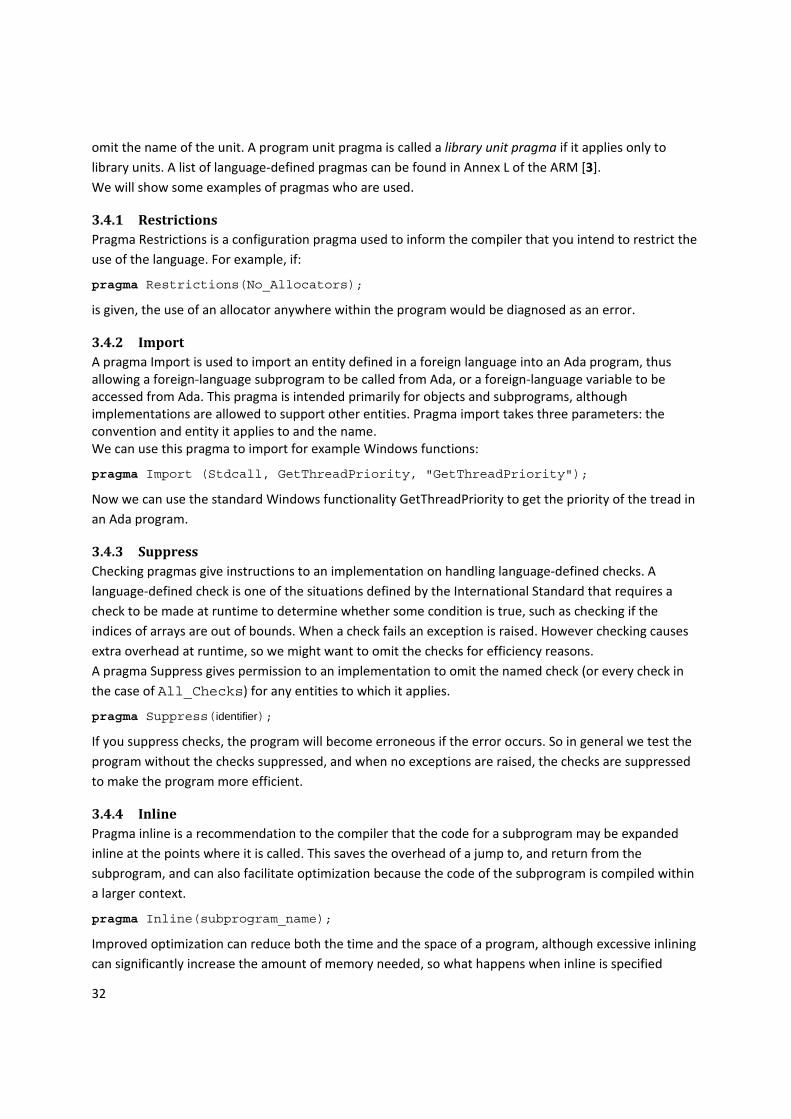
3.4 Pragmas Pragmas are directives to the compiler. Special rules apply to the placement of certain pragmas. Configuration pragmas apply to an entire program. The pragma declaration is itself a compilation unit, which is normally the first unit that is compiled.  A program unit pragma applies only to a single program unit. Such pragmas can be placed either within the unit they apply to or after the unit. If the pragma is the first entity within a unit, you can sometimes 

32  

omit the name of the unit. A program unit pragma is called a library unit pragma if it applies only to library units. A list of language‐defined pragmas can be found in Annex L of the ARM [3].  We will show some examples of pragmas who are used. 

3.4.1 Restrictions Pragma Restrictions is a configuration pragma used to inform the compiler that you intend to restrict the use of the language. For example, if: 

pragma Restrictions(No_Allocators);

is given, the use of an allocator anywhere within the program would be diagnosed as an error. 

3.4.2 Import A pragma Import is used to import an entity defined in a foreign language into an Ada program, thus allowing a foreign‐language subprogram to be called from Ada, or a foreign‐language variable to be accessed from Ada. This pragma is intended primarily for objects and subprograms, although implementations are allowed to support other entities. Pragma import takes three parameters: the convention and entity it applies to and the name. We can use this pragma to import for example Windows functions: 

pragma Import (Stdcall, GetThreadPriority, "GetThreadPriority");

Now we can use the standard Windows functionality GetThreadPriority to get the priority of the tread in an Ada program. 

3.4.3 Suppress Checking pragmas give instructions to an implementation on handling language‐defined checks. A language‐defined check is one of the situations defined by the International Standard that requires a check to be made at runtime to determine whether some condition is true, such as checking if the indices of arrays are out of bounds. When a check fails an exception is raised. However checking causes extra overhead at runtime, so we might want to omit the checks for efficiency reasons. A pragma Suppress gives permission to an implementation to omit the named check (or every check in the case of All_Checks) for any entities to which it applies. 

pragma Suppress(identifier);

If you suppress checks, the program will become erroneous if the error occurs. So in general we test the program without the checks suppressed, and when no exceptions are raised, the checks are suppressed to make the program more efficient. 

3.4.4 Inline Pragma inline is a recommendation to the compiler that the code for a subprogram may be expanded inline at the points where it is called. This saves the overhead of a jump to, and return from the subprogram, and can also facilitate optimization because the code of the subprogram is compiled within a larger context. 

pragma Inline(subprogram_name);

Improved optimization can reduce both the time and the space of a program, although excessive inlining can significantly increase the amount of memory needed, so what happens when inline is specified 

33  

should be measured. Some compilers can turn inlining on and off by using a compiler switch and some compilers performs inlining automatically. We have a compiler switch ‘‐gnatn’ for gcc who activates inlining for all subprograms for which pragma inline is specified. The use of inlining can better be deferred until late in the development of a program. The reason is that recompilation of a package body containing an inlined subprogram may require recompilation of every unit that depends on the package specification, even if the subprogram body was not modified. Pragma Inline_Always is an additional defined pragma defined by GNAT. Pragma Inline_Always is similar 

to pragma Inline except that inlining is not subject to the use of option `-gnatn' and the inlining happens regardless of whether this option is used [23]. 

pragma Inline_Always (subprogram_name);

 

34  

4 SCHEDULING 

The applications build for the equipment made by ITEC have about 30‐100 threads. When more than one thread is ready to run at the same time, some kind of scheduling is needed. In this chapter we describe the concepts related to scheduling. In section 4.1 we will look at the objects which can be scheduled. Section 4.2 presents some general points about scheduling threads and section 4.3 about priorities. Sections 4.4 and 4.5 describe how Windows and Ada handle scheduling. 

4.1 Objects When talking about scheduling, we have different concepts used for slightly different purposes. We have programs and processes, threads, tasks and jobs. In this section we will explain what these mean and how we use them. 

4.1.1 Programs, processes and threads A program is a static sequence of instructions, whereas a process is a container for a set of resources used when executing the instance of the program. A process is a collection of one or more threads and associated system resources (such as memory containing code and data, open files, and devices). For instance, in Windows a newly created process is started with a single thread which can create additional threads [15]. A thread is the entity within a process that is allocated processor time and scheduled for execution [7]. A thread includes a processor context (this includes the program counter and stack pointer) and its own data area for a stack (to enable subroutine branching). A thread executes sequentially and is interruptible so that the processor can turn to another thread [29]. Multithreading refers to the ability of an operating system to support multiple threads of execution within a single process. By breaking a single application into multiple threads, the programmer improves the modularity of the application and has more control over the timing of application‐related events [6]. 

4.1.2 Tasks In Ada each task is mapped on an underlying kernel thread [23]. The advantage of mapping each task to an underlying thread is among other things that the scheduler of the operating system can be used to schedule the Ada tasks. Mostly, the terms thread and task are used interchangeable. A task can have a deadline, a ready time, a processing time, resource requirements, a priority and a period [6]. The deadline of a task is an upper bound on the start or completion time of the task after it became ready to execute. Although a deadline can indicate a start or completion time, most of the times it is used to specify the completion time.  Tasks can be classified into four basic levels of criticality according to the importance of meeting its deadline. A hard deadline task is one that must meet its deadline. The failure of such a task to meet its deadline may result in an unacceptable failure at the system level. Firm and soft deadline tasks are tasks that must meet their deadline under normal conditions. An occasional missed deadline can be tolerated without causing system failure, but may result in degraded system performance. For a firm deadline task there is no value in completing it after its deadline. For soft deadline tasks it is valuable to complete it 

35  

after its deadline. A non‐critical task has no strict deadline. Such a task is typically a background task that performs activities such as system logging. Failure of a non‐critical task does not endanger the performance of the system [11]. At the ITEC machines there are only a couple of tasks with hard deadlines. Tasks can be periodic or aperiodic. A periodic task becomes ready to execute periodically after a specified amount of time. An aperiodic task becomes ready to execute after a certain event occurs [6]. On the ITEC machines there are both periodic and aperiodic tasks. 

4.1.3 Jobs In the description of priority inheritance protocols, often the term ‘job’ is used. A job is a sequence of instructions that will continuously use the processor until its completion if it is executing alone on the processor. So a job will not suspend it selves, this effect can be accommodated by defining two or more jobs. So a periodic task is a sequence of the same type of job occurring at regular intervals [30]. Therefore a job can be an entire task, or just a part of the task. In this thesis we however do not make explicit difference between periodic and sporadic tasks. A task can become ready because of a timing event or some other event. Because of that, we only use the notion of task and not of job. 

4.2 Executing threads A thread can be in various execution states. A thread is ready when it is waiting to execute. When a thread is actually being executed, it is said to be running. At one processor only one thread can be running at a time. A thread is waiting when it is not ready to execute, for instance, because it is waiting for some synchronization or time event to happen. This state is also called suspended or blocked [5]. A switch between different threads is called a context switch. The machine state associated with the current running thread is saved, another thread’s state is loaded and the new thread is started for execution. At which point a context switch can take place and which task will be scheduled next, depends on the scheduling policy in use. The process by which one ready thread is selected for execution on a processor is called dispatching [3]. There are two general categories of decision modes of when a context switch can be performed, nonpreemptive and preemptive. In the case of nonpreemptive, once a task is running, it continues to execute until it terminates or it blocks itself. In the preemptive case, the currently running task may be preempted by the scheduler. The tasks running on the ITEC machines can be preempted. Normally the functional correctness of a concurrent program should not depend on the exact order in which tasks are executed. But a real‐time program has requirements related to timing that can dictate the order in which events must occur and be handled. Real‐time scheduling is therefore concerned with controlling the order of execution of tasks [5].   

4.3 Priorities The priority of a task is a value that indicates a degree of urgency of that task. It is often used as the basis for resolving competing demands of tasks for resources. Whenever tasks compete for processor time or other resources, the resources are allocated to the task with the highest priority value [3]. With a preemptive decision mode, the scheduler ensures that the highest priority ready task is always executing. If a task with a priority higher than the currently running task becomes ready, the scheduler will perform a context switch, to enable the higher priority task to execute [11].  

36  

Priorities can be assigned by the developer on beforehand, or can be assigned through analyzing the system by an algorithm. At ITEC the priority of the tasks is determined in advance, following the categorization in Table 1. Logging tasks have a low priority and control tasks have a high priority. All tasks are in the same process, which has to be real‐time. So the priorities of the tasks are all in the real‐time priority class of windows XP (see section 4.4.1).  Priority level 

Task category 

2  Motion planning 

1  Other important tasks 

0  Control tasks 

‐1  CPU intensive tasks 

‐2  Visual ITEC Table 1: ITEC priority levels 

Priorities can be assigned statically or dynamically. With static or fixed priority approaches, the priority of a task is not changed at runtime by the scheduler.  Usually a schedulability analysis of the system is performed and the results of this analysis are used to assign priorities to the tasks. With dynamic priority scheduling, the priorities of the tasks may change during the execution of the system. When the resource requirements are known, processor load for example, it is possible to analyze a program and decide if it will meet all its timing requirements. Two widely used methods for scheduling and analysis of real‐time systems are Rate Monotonic scheduling and Earliest Deadline First. With these algorithms the total processor utilization can be computed on beforehand, and when this is below a certain upper bound, the algorithm guarantees that all tasks are scheduled such that they all meet their deadlines [6].  

4.3.1 Rate Monotonic Scheduling Rate Monotonic (RM) scheduling can be used for periodic tasks. This algorithm assigns fixed priorities to tasks on the basis of their periods. The highest‐priority task is the one with the shortest period. And the lowest priority task is the one with the longest period. The rate of a task is the inverse of the period of a task. So the priority of the tasks is a monotonically increasing function of their rates [6]. 

4.3.2 Earliest Deadline First The Earliest Deadline First (EDF) algorithm is a dynamic priority scheduling algorithm. With EDF the task which is closest to its deadline is scheduled. When a collection of tasks does not use more than 100% of the processor time, EDF leads to a correct schedule on a preemptive uniprocessor. Therefore it is an optimal scheduling algorithm. However EDF does not take priorities into account. So when the collection of tasks cannot be scheduled because the total utilization is more than 100%, the set of tasks that will miss deadlines is unpredictable. This is in contrast to fixed priority scheduling algorithms like RMS where the low‐priority tasks will miss their deadlines, which gives fewer problems. 

37  

4.4 Windows Windows implements a preemptive scheduler with a flexible system of priority levels. We will first discuss the priority levels in section 4.4.1. In section 4.4.2 we will describe how Windows schedules the threads. 

4.4.1 Priority levels There are separate kernel and application priorities. Application priorities are organized into two classes: real‐time and variable. In Figure 15 these application priority levels are shown together with the kernel priority levels. 

In the variable priority class, a thread’s priority begins at some initial assigned value and may be temporarily raised during the thread’s lifetime. However it can never be raised to the real‐time priority class. This raising is sometimes done by the scheduler to prevent starvation. In the real‐time priority class, all threads have a fixed priority that will not be changed automatically by the system [29]. We can however change the priority of a thread by calling the windows API function SetThreadPriority.  The priority of each thread is determined by the priority class of its process and the priority level of the thread within the priority class of its process. These two criteria are combined to form the base priority of a thread. There are six priority classes for processes: REALTIME_PRIORITY_CLASS (24), HIGH_PRIORITY_CLASS (13), ABOVE_NORMAL_PRIORITY_CLASS (10), NORMAL_PRIORITY_CLASS (8), BELOW_NORMAL_PRIORITY_CLASS (6) or IDLE_PRIORITY_CLASS (4). The SetPriorityClass function sets the priority class for a process. The GetPriorityClass function can be used to determine the current priority class of a process [15]. The priority class of a process determines the base priority of the threads belonging to that process. 

DIRQL HardwareInterrupts

IRQL SoftwareInterrupts

Real‐TimeLevels 

VariableLevels

Application 

Kernel 

High 

 

Interprocessor Interrupt 

Clock 

Device Interrupt 

… 

Device Interrupt 

DISPATCH_LEVEL 

APC_LEVEL 31 

… 16 

15 

… 

1 

0 

Figure 15: Windows priority levels

38  

Within each priority class are seven priority levels for threads: THREAD_PRIORITY_IDLE (‐15), THREAD_PRIORITY_LOWEST (‐2), THREAD_PRIORITY_BELOW_NORMAL (‐1), THREAD_PRIORITY_NORMAL (0), THREAD_PRIORITY_ABOVE_NORMAL (+1), THREAD_PRIORITY_HIGHEST (+2) and THREAD_PRIORITY_TIME_CRITICAL (+15). The numbers between brackets indicate the relative priority of the thread to the priority class of the process. When threads are created they have the priority THREAD_PRIORITY_NORMAL, which means it is the base priority of the process class. In Figure 16 the relation between priority classes, thread priorities and the actual priorities used for scheduling can be seen.  Priority class  REALTIME  HIGH  ABOVE 

NORMAL NORMAL BELOW 

NORMAL IDLE

Scheduling Priority 

31  TIME CRITICAL           

26  HIGHEST           

25  ABOVE NORMAL           

24  NORMAL           

23  BELOW NORMAL           

22  LOWEST           

16  IDLE           

15    TIME CRITICAL HIGHEST 

TIME CRITICAL  TIME CRITICAL  TIME CRITICAL  TIME CRITICAL 

14    ABOVE NORMAL        

13    NORMAL         

12    BELOW NORMAL HIGHEST       

11    LOWEST  ABOVE NORMAL      

10      NORMAL  HIGHEST     

9      BELOW_NORMAL ABOVE NORMAL    

8      LOWEST  NORMAL  HIGHEST   

7        BELOW NORMAL ABOVE NORMAL   

6        LOWEST  NORMAL  HIGHEST 

5          BELOW NORMAL  ABOVE NORMAL

4          LOWEST  NORMAL 

3            BELOW NORMAL

2            LOWEST 

1    IDLE  IDLE  IDLE  IDLE  IDLE 

0             

Figure 16: Windows thread priorities 

The SetThreadPriority function can be used to change the priority value of a thread, but it has to stay in between THREAD_PRIORITY_IDLE and THREAD_PRIORITY_TIME_CRITICAL of the priority class of the process. For example, a thread belonging to a process in the normal priority class cannot get a priority of thirteen. 

39  

4.4.2 Scheduler Scheduling decisions are made based on the current priority of the thread [7]. The system treats all threads with the same priority as equal. All of the active threads at a given priority level are in a round‐robin queue (See Figure 17). With Round Robin Scheduling, each task is given a time quantum. When a task is being executed, this time is used. When the task is out of time, it is placed at the end of the ready queue, and the next ready thread is selected. This technique is also known as time slicing, because each process is given a slice of time before being preempted [6].    

 Figure 17: Windows Thread Dispatching Priorities [29] 

The system first assigns time slices to all threads with the highest priority. If none of these threads are ready to run, the system assigns time slices to all threads with the next highest priority. If a higher‐priority thread becomes available to run, the system stops executing the lower‐priority thread, puts it back at the front of its priority ready queue, and assigns a full time slice to the higher‐priority thread [15]. 

40  

However, it is not entirely clear whether this also holds for threads in the real‐time class. A number of sources [6][29][31] state that windows uses a round‐robin system, but it is not made explicit that this also applies to the real‐time class. However we know that high priority threads get precedence to low priority threads, we just do not know for certain how threads of the same priority are scheduled. So we should not depend on a certain scheduling policy within priority levels. 

4.5 Ada In Ada the task dispatching policy can be set with the pragma Task_Dispatching_Policy. According to Annex D of the ARM [3] there are four dispatching policies available: FIFO_Within_Priorities, Non_Preemptive_FIFO_Within_Priorities, Round_Robin_Within_Priorities and EDF_Across_Priorities. The term “Within priorities” indicates that the policy is used when more than one task has the same priority to determine which task will run first. Policy EDF_Across_Priorities always schedules the task which is closest to its deadline first, regardless of its priority. However, since the GNAT implementation just maps the Ada tasks to Windows threads, the windows scheduler is used and the mentioned Ada dispatching policies are not available. 

4.5.1 Priorities According to the Real‐Time Systems Annex of Ada, at least 30 priority values and one interrupt priority are required [3]. GNAT defines 31 priorities, ranging from 0 up to and including 30 and an interrupt priority with value 31. When no priority is specified for a task, a default priority is used with a value of 15. 

subtype Any_Priority is Integer range 0 .. 31; subtype Priority is Any_Priority range 0 .. 30; subtype Interrupt_Priority is Any_Priority range 31 .. 31; Default_Priority : constant Priority := 15;

The Ada task priorities map onto the underlying thread priorities. But because there are only seven priority levels available in Windows NT and sixteen in Windows 2000/XP (the variable or the real‐time priority classes of Figure 17), compression is used for the mapping. These priorities and the mapping can be found in the file system.ads of the GNAT run‐time components: 

type Priorities_Mapping is array (Any_Priority) of Integer; Underlying_Priorities : constant Priorities_Mapping := (Priority'First .. Default_Priority - 8 => -15, Default_Priority - 7 => -7, Default_Priority - 6 => -6, Default_Priority - 5 => -5, Default_Priority - 4 => -4, Default_Priority - 3 => -3, Default_Priority - 2 => -2, Default_Priority - 1 => -1, Default_Priority => 0, Default_Priority + 1 => 1, Default_Priority + 2 => 2, Default_Priority + 3 => 3, Default_Priority + 4 => 4, Default_Priority + 5 => 5, Default_Priority + 6 ..

41  

Priority'Last => 6, Interrupt_Priority => 15);

This mapping means that the Ada priorities 0 until 7 are mapped to Windows priority ‐15 (IDLE, that is 1 or 16 depending on the priority class of the process). Ada priorities 8 until 14 are mapped to the Windows priorities ‐7 until ‐1. The Default_Priority of 15 is mapped to Windows priority 0 (NORMAL). Ada priorities 16 until 20 are mapped to Windows priority 1 until 5. Ada priorities 20 until 30 are mapped to Windows priority 6. And the Interrupt_Priority (31) is mapped to windows priority 15. These mapping priority are the Windows thread priorities relative to the priority class of the process. For example, an Ada priority of 17 for a task from a process in the real‐time priority class is mapped to a windows thread priority of 2. The real‐time priority class means a base priority of 24, with the additional 2 it becomes a scheduling priority of 26. In Ada a task’s initial priority is set by including a pragma (See 3.4) in its specification: 

pragma Priority(expression);

A Priority pragma can be used within a task definition (3.1.4), a protected definition (3.1.5), or the declarative part of the subprogram body of the main subprogram. 

task TaskA is pragma Priority(System.Default_Priority + 1);

end TaskA;

If a task‐type definition contains such a pragma, then all tasks of that type will have the same priority unless a discriminant is used (Entries will be explained in 5.5.3.): 

task type Servers(Task_Priority : System.Priority) is entry Service1(...); entry Service2(...); pragma Priority(Task_Priority);

end Servers;

The initial base priority of a task in the absence of a pragma is the base priority of the task that creates it at the time of creation. If there is no pragma Priority in the main subprogram, the initial base priority of the environment task is the default priority of the system. After a task is created, its base priority can be changed only by a call to Dynamic_Priorities.Set_Priority [3].  

42  

5 DATA SHARING 

In Ada, if several tasks are declared within a subprogram or package, they can all read and write variables declared previously in the enclosing declarative region. Such variables are called shared variables. Similarly, sharing of variables can occur if a subprogram that reads or writes a global variable is called by several tasks. Shared variables can be found in all kind of programs, not just in Ada programs. Normally, sharing variables should be avoided, because they can introduce all kind of consistency problems. But sometimes shared variables are used for communication between tasks, and cannot be left out for the correct working of the program. At these points some kind of technique should be used to guarantee the consistency of the shared variables. In the next section we will first see what is meant by mutual exclusion. Then interlocked operations 5.2 and spinlocks (5.3) are discussed. Windows and Ada both contain mechanisms that can be used for communication between tasks and correct sharing of variables. We will discuss these at the end of the chapter (5.4 and 5.5). 

5.1 Mutual exclusion Mutual exclusion is the guarantee that one, and only one, thread can access a particular resource at a time. Mutual exclusion is necessary when a resource does not lend itself to shared access or when sharing would result in an unpredictable outcome. For instance, while one thread is writing to a file, updating a database, or modifying a shared variable, no other thread can be allowed to access the same resource [7]. Sections of code that access a non‐sharable resource are called critical sections. Critical sections can be protected from concurrent access by locking a synchronization object, like a mutex (see 5.4.1), at the beginning of the section and unlocking it at the end [32]. A possible way to achieve mutual exclusion is to disallow that a task in a critical section is pre‐empted. Then no other task can access the shared resource before the first task is finished with its critical section. This method does not work for multiprocessor systems, because tasks can run in parallel without the need for preemption, still allowing more than one task accessing the same variable at the same time. So we need another way to achieve mutual exclusion. 

5.2 Interlocked operations Interlocked functions provide a simple mechanism for synchronizing access to a variable that is shared by multiple threads. They rely on hardware support for multiprocessor‐safe manipulating integer values and performing comparisons. For example the x86 assembly instruction lock xadd locks the multiprocessor bus before it executes the xadd instruction (adding the two operands and storing the result in the destination operand). This way another thread that also wants to use this variable is prevented from accessing the same memory address and will not be able to modify the variable between the read of the original value and the write of sum value [7]. The Windows API also contains support for interlocked functions. This includes functions as InterlockedDecrement, InterlockedIncrement, InterlockedExchange, InterlockedExchangePointer, 

43  

InterlockedCompareExchange, InterlockedCompareExchangePointer, InterlockedAnd, InterlockedOr and InterlockedXor. Furthermore there are some functions that are specifically designed for 64‐bit systems. These functions use the assembly instructions of the system. The InterlockedDecrement function, for example, uses the x86 instruction lock xadd through adding minus one. More information on specific functions can be found on the Microsoft Developer Network [15]. The threads of different processes can use these functions if the variable is in shared memory, to prevent synchronization problems. These functions can also be used to build more complex synchronization objects like mutexes as we will see in chapter 7. The interlocked functions can execute extremely quickly because no transition from user mode to kernel mode is needed [31]. 

5.3 Spinlocks A spinlock is a locking primitive associated with a global data structure. Before entering a critical section, the spinlock must be acquired. If the spinlock is not free, the thread keeps trying to acquire the lock until it succeeds. The spinlock gets its name from the fact that the processor keeps "spinning" until the thread gets the lock. On many architectures, spinlocks are implemented with a hardware‐supported test‐and‐set operation, which tests the value of a lock variable and acquires the lock in one atomic instruction. Testing and acquiring the lock in one instruction prevents a second thread from grabbing the lock between the time when the first thread tests the variable and the time when it acquires the lock. A spinlock should be used with care, minimizing the number of instructions executing while holding a spinlock, because another thread may be busy waiting for it [7]. The use of spinlocks should be avoided on uniprocessor systems, because when one thread is keeping the processor busy, waiting for the resource, the thread keeping the resource does not get time to release it. 

5.4 Windows mechanisms Windows provides some mechanisms that threads can use to synchronize access to a resource. The user‐visible synchronization objects acquire their synchronization capabilities from dispatcher objects. Dispatcher objects are kernel objects added to the executive for synchronization. When a user application uses such a synchronization object, a switch to kernel mode is made. The operating system executes the corresponding instructions and switches back to user mode before returning control back to the user thread [7]. We will discuss some of these synchronization objects in the next sections. 

5.4.1 Semaphore  A Windows semaphore object is a synchronization object that maintains a count between zero and a specified maximum value. It is a counter that regulates the number of threads that can use a resource. The count is decremented each time a thread obtains access to the semaphore and incremented each time a thread releases the semaphore. The state of a semaphore is signaled when its count is greater than zero and nonsignaled when its count is zero. When the count reaches zero, additional threads have to wait until another thread releases the semaphore and sets the state to signaled [15]. Semaphore objects may be shared by threads in multiple processes [29]. 

44  

5.4.2 Mutex Mutex is an abbreviation of mutual exclusion. A mutex object is used to provide mutually exclusive access to a resource, allowing only one thread object at a time to gain access. A thread that needs the resource must lock the mutex before using the resource. After using the resource, the mutex is unlocked to allow another thread access to the resource. A Windows mutex object functions as a binary semaphore. The owning thread or another tread can release the mutex. When the mutex object is released, only one thread can now acquire the mutex. Mutexes, like semaphores, can be used to synchronize threads running in different processes, unlike critical section objects (see 5.4.3) which can only be used for threads in the same process [29]. 

5.4.3 Critical section objects The Windows API contains a Critical Section Object. Critical sections provide a synchronization mechanism similar to that of mutex objects. The difference is that critical sections can be used only by the threads of a single process and they are much faster and efficient for mutual‐exclusion synchronization, especially on multiprocessor systems. This is caused by the way critical sections are implemented. On multiprocessor systems, the thread will attempt to acquire a spinlock (see 5.3) before performing a wait operation on a semaphore that is associated with the critical section. If the critical section becomes free during the spin operation, the calling thread avoids the wait operation. An advantage of a critical section compared to a mutex object is that if there is no contention, then no transition made to kernel mode is made. Effectively the spinlock optimizes for the case where the thread that currently owns the critical section is executing on another processor. On single‐processor systems, no spinning is done [15] [29]. A process can declare a variable of type CRITICAL_SECTION. Before this variable can be used, some thread of the process must initialize it by calling the InitializeCriticalSection function. After the variable is created, a thread can call the EnterCriticalSection function to request ownership of the critical section. This has to be done before executing any section of code that accesses a protected resource. This way mutually exclusive access to that shared resource is provided. The EnterCriticalSection function waits for ownership of the specified critical section object. The function returns when the calling thread is granted ownership. After a thread has ownership of a critical section, it can make additional calls to EnterCriticalSection without blocking its execution. This prevents a thread from deadlocking itself while waiting for a critical section that it already owns. Besides the EnterCriticalSection function, there is also a TryEnterCriticalSection. This function attempts to enter a critical section without blocking. If the call is successful, the calling thread takes ownership of the critical section. If it is unsuccessful, it is not going to wait. When a thread has finished executing the protected code, it uses the LeaveCriticalSection function to release the ownership of the critical section, enabling another thread to become owner and access the protected resource. The thread must call LeaveCriticalSection once for each time that it entered the critical section. If a thread terminates while it still has ownership of a critical section, the state of the critical section is undefined. 

5.4.4 Handles and Objects A Windows object is a data structure that represents a system resource, such as a file, graphic image, thread, semaphore or mutex. An application cannot directly access object data or the system resource 

45  

that an object represents. Instead, an application must obtain an object handle [15]. A handle is a unique identifier assigned to an entry in a table inside the kernel. In this table are all the different objects that the kernel is responsible for. This table is maintained by Windows itself. If you want an entry out of the table, you need to give Windows the handle value [33]. A handle to the object is obtained when the object is created. For example the function CreateMutex returns a handle to a newly created mutex. The DuplicateHandle function duplicates an object handle. The duplicate refers to the same object as the original handle. DuplicateHandle ensures that the reference count is increased when a handle is duplicated. So that when a handle is passed to another thread, the object will not be destroyed until both threads have closed the handle. When a process uses the GetCurrentProcess function or a thread uses the GetCurrentThread function to get a handle to itself, it is a pseudo handle. It can be used to access the object, but it is not maintained in the kernel table. The DuplicateHandle function converts it to a real process or thread handle. The CloseHandle function closes an open object handle. It should be used when you are finished with the object. CloseHandle invalidates the specified object handle, decrements the object’s handle count and performs object retention checks. The documentation [15] for the functions that creates a specific object indicate exactly what happens after the handle is closed. After the last handle to an object is closed, the object is removed from the system. Closing a handle to a thread or process does not terminate the associated thread or process or remove it. To remove a thread or process object, you must terminate the thread or process and then close all handles to it [15]. 

5.5 Ada mechanisms In Ada, there are three main constructs for writing good concurrent programs [8]: 

• Rendezvous for direct task‐to‐task synchronous communication. • Protected objects for asynchronous sharing of resources. • Direct use of shared variables.  

Atomic variables (5.5.1) and volatile objects (5.5.2) are used for direct use of shared variables. Protected objects will be described in section 5.5.4 and rendezvous in 5.5.3. 

5.5.1 Atomic variables One of the problems of concurrent access to shared variables is when the variable is not atomic. This is likely if more than one memory word is needed to store the variable, such as with high‐precision floating point numbers and with arrays of records. Suppose that a task updates one word of a two‐word variable and then it is preempted by another task that updates both words of the same variable. When the first task is resumed, it will update the second word, leaving the variable with a mixture of two values. Normally, the variables should be encapsulated in protected objects or tasks. But if efficiency is important, the direct use of shared variables can be required. We may want to read and update shared variables without the overhead of rendezvous or protected actions but also without the problems of accessing them concurrently [8]. In Ada, two actions can be sequential when they are, for example, part of the execution of the same task. Two actions on the same (shared) object can be erroneous unless the actions are sequential. 

46  

We can use the pragma Atomic to specify that an object is atomic. For an atomic object all reads and updates of the object as a whole are indivisible. If two actions are the read or update of the same atomic object, the two actions are sequential [3].   Not all objects can be accessed atomically. When an object cannot be accessed atomically, we will have to use other means to ensure that the object contains a consistent value. 

5.5.2 Volatile objects Another problem with shared variables is when code generators make assumptions that may not be valid in the presence of concurrency. For example when updating a variable and then using it again in an operation. In between the variable could stay in the register without being written to memory. But meanwhile another task can use the old value from memory. In Ada we can use pragma Volatile to prevent this. For a volatile object all reads and updates of the object as a whole are performed directly to memory. Volatile can be used on a compound object that cannot be accessed atomically, but it does not make the object atomic [8]. Every atomic type or object is also defined to be volatile [3]. 

5.5.3 Rendezvous Rendezvous is the primary communication mechanism of tasks in Ada83, when protected objects did not yet exist. Tasks can communicate synchronously when using task entries. An entry is declared in the task declaration. Another task can call this entry. The calling task and the called task must execute a rendezvous at an accept statement. The first party to reach the rendezvous point must wait until the second party arrives. During a rendezvous the sequence of statements in the accept statement is executed. After a rendezvous, the two tasks continue their execution independently. As an example, consider the following Ada program 

with Ada.Text_IO; use Ada.Text_IO; procedure Rendezvous is task A is entry Synchronize; end A; task body A is begin Put_Line ("Task A doing something before synchronizing"); accept Synchronize do Put_Line ("Synchronized"); end Synchronize; Put_Line ("Task A doing something after synchronizing"); end A; task B; task body B is begin Put_Line ("Task B doing something before synchronizing"); A.Synchronize; Put_Line ("Task B doing something after synchronizing"); end B; begin null; end Rendezvous;

When executed this program might output: 

47  

Task B doing something before synchronizing Task A doing something before synchronizing Synchronized Task B doing something after synchronizing Task A doing something after synchronizing

The order of the A and B actions before and after synchronization depends on how the tasks are scheduled.  Because Ada 83 only supports the notion of a task, active entities, but also all control entities were encoded in tasks. To protect a shared resource, a server task is created. When a task wants to access the shared resource, it calls an entry of the server task. Once the task has synchronized with the sever task, it can access the shared resource. 

5.5.4 Protected Objects Ada 95 introduced a new abstraction for resource entities, who do not need a thread of control themselves, namely the protected type. An object of such a type can control access to the data it protects but does not have a thread of control. Protected objects are passive and just “sit there”, waiting till their entries and subprograms are called. The use of protected objects for resources is much more efficient than the use of tasks, because much less context switches are needed. Thus resources should be coded as protected objects, with tasks being used for active objects and servers [5].  The difference between a protected unit and a package is that the subprograms of a package can be called concurrently from multiple tasks, possibly leading to race conditions. The operations of a protected unit are mutually exclusive, meaning that only one will be executed at a time [8]. Tasks can only access the data of the protected object through a protected operation.    

48  

6 PRIORITY INHERITANCE PROTOCOLS 

When a low‐priority task has locked a synchronization object, for example a mutex, which is also needed by a higher priority task, in that case, the higher priority task cannot access the resource and therefore has to enter the wait state. The high‐priority task is kept from executing by a low‐priority task that is running. The order of execution has been subverted with respect to the priorities of the task. Therefore this is called priority inversion [5]. The lower‐priority task is said to block the higher‐priority task. Unbounded priority inversion occurs when the lower‐priority task cannot finish its critical section as fast as possible because it is preempted by some medium priority tasks. The execution time of these tasks can be unboundedly long, while in the meantime the high priority task is still waiting for the low‐priority task to unlock the mutex. An example of this is shown in Figure 18.       

  Running       Attempts to lock M   

           

TH  Ready             

  Waiting        

  Running            

           

TM  Ready             

  Waiting            

  Running Locks M  Preempted       

 

Critical section        

TL  Ready             

  Waiting          

Figure 18: Priority inversion 

Priority inversion cannot be entirely removed as the integrity of the protected data must be ensured [5]. But priority inversion can be bounded. A possible solution for unbounded priority inversion is to disallow that a task in a critical section is pre‐empted. This way the critical section is executed as fast as possible. This solution is only appropriate for very short critical sections, because it prevents high priority tasks from running immediately when ready. Especially in time critical systems, it is important for high priority tasks to be scheduled fast.  It also needlessly blocks tasks which do not need to access the shared data structure currently in use [30]. The same problems arise when critical sections are always executed on the highest priority level. More suitable to solve the unbounded priority inversion problem is the use of some sort of priority inheritance protocol. Under a priority inheritance protocol tasks do not always execute at their normal assigned priority. Priority inheritance allows a task to execute with an enhanced priority if it is blocking (or could block) a higher‐priority task [5]. It inherits the priority of the higher‐priority task. A task can only 

49  

block another task while executing in a critical section. After exiting its critical section, the task returns to its original priority level [32]. There are different priority inheritance protocols. These protocols mainly differ on when the priority of a task is raised and when a task may lock a mutex. Furthermore, some protocols also solve some other problems. In this chapter we present a number of these protocols. 

6.1 Basic priority inheritance protocol (PIP) For the basic priority inheritance protocol most things are the same as just using mutexes without priority inheritance. A task TK can preempt another task TL if task Tk is ready and its priority is higher than the priority at which task TL is executing. When a task TH is currently running and it wants to enter a critical section, it must first lock a mutex guarding the critical section. When the mutex is not locked, task TH will lock it and enter its critical section. When this mutex was already locked, say by task TL, task TH has to wait and is now blocked by TL. If TH‘s priority is higher than that of TL, TL inherits the priority of TH. When TL exits its critical section, the mutex will be unlocked and TL resumes execution at the priority it had at the point of entry into the critical section. Next, a higher priority task waiting for the mutex can pre‐empty the execution of TL and lock the mutex. In Figure 19 we see the example from Figure 18, but now with PIP applied. The high priority task still has to wait until the low priority task is finished with the mutex, but is not interfered anymore by medium priority tasks. 

  Running      Attempts to lock M Locks M           Critical 

Section 

 

TH  Ready               

  Waiting              

  Running              

             

TM  Ready              

  Waiting  

             

  Running  Locks M  Preempted Priority raised Unlocks M   Critical 

section 

    Critical Section 

   

TL  Ready              

  Waiting  

             

Figure 19: Preventing unbounded priority inversion with the basic priority inheritance protocol 

Priority inheritance is transitive. So if TH is blocked by TM and TM is blocked by TL, TL inherits the priority of TH via TM. The operations of priority inheritance and of the resumption of the original priority must be indivisible. This is to maintain consistency of the internal data structures used for the inherited priority.  With priority inheritance, a low priority task can only block a higher priority task in two situations. The first is when the low priority task has locked the mutex and the high priority task want to lock it. This is called direct blocking. This kind of blocking is needed to ensure the consistency of the shared data the mutex protects. Second, when a low priority task TL has inherited a high priority from a high priority task TH which it blocks, TL can block a medium priority task TM. This is called push‐through blocking. It is needed to avoid task TH being indirectly preempted by the medium priority task.  

50  

The basic priority inheritance protocol bounds the priority inversion, because a high priority task can only be blocked by a lower priority task for at most the duration of the critical section. For Ada, only Ceiling Locking (see 6.5) is required by the Real‐Time Systems Annex, but an implementation may define other locking policies. So GNAT has included PIP as an implementation‐defined locking policy named Inheritance_Locking. It can be used by including: 

pragma Locking_Policy (Inheritance_Locking);

On targets that support this policy, locking is implemented with the priority inheritance protocol [23]. Windows does not support priority inheritance, so this locking policy is not implemented for Windows. 

6.2 Deadlock and multiple blocking The basic priority inheritance protocol does not solve two other problems, namely the possibility of deadlocks and multiple blockings. Deadlock can occur when tasks need multiple resources at the same time. For example (see Figure 20) when task TL locks mutex M1 and also needs mutex M2, but before it can do that it is preempted by a higher priority task TH. Task TH locks M2 and also needs M1, but cannot lock it because it is already locked by task TL. Task TL now inherits the higher priority of task TH but it cannot lock M2 because that one is still locked by task TH, thus a deadlock has arisen. [30]  

  Running     Locks M2 Attempts to lock M1    

             

TH  Ready         Deadlock    

  Waiting              

  Running Locks M1  Preempted  Priority raised  Attempts to lock M2  

 

          

TL  Ready            Deadlock  

  Waiting              

Figure 20: Example of deadlock with the basic priority inheritance protocol 

Multiple blocking can occur when a task needs two or more mutexes which all are already locked by other tasks. The task is now multiple blocked and has to wait until all of these tasks are done with all those mutexes.  

6.3 Priority Ceiling Protocol (PCP) The goal of the priority ceiling protocol is to avoid, in addition to priority inversion, deadlocks and multiple blocking [4]. Under the priority ceiling protocol, each mutex will be given a ceiling priority. This ceiling priority is the highest priority of all tasks that use this mutex. When a task T tries to lock a mutex that is not yet locked, it only succeeds if the priority of task T is higher than the priority ceiling of all the mutexes currently locked by tasks other than task T. When this is not the case, task T has to wait and is said to be blocked by the task currently holding the lock of the mutex with the highest priority ceiling. When a task blocks higher priority tasks, when holding a lock on a mutex, the task inherits the highest priority of the tasks it blocks [30]. 

51  

With this protocol deadlock is prevented. In Figure 21 we see the same example from Figure 20, but now with PCP. TL locks mutex M1 and also needs mutex M2. Before it can do this, it is preempted by higher priority task TH which wants to lock M2 and successively M1. Now the priority ceiling of M1 is at least equal to the priority of TH. So task TH is now refused the lock on M2, because the priority of TH is not higher than the priority ceiling of all mutexes currently locked, in this case M1 which is locked by TL. TH is blocked by TL, so TL inherits the priority of TH and TL can resume trying to lock M2 which is not already locked by TH, so deadlock is prevented.  

  Running     Attempts to lock M2 Locks M2  Locks M1   

             

TH  Ready            

  Waiting              

  Running Locks M1  Preempted  Priority raised  Locks M2 Unlocks M2 Unlocks M1   

 

            

TL  Ready               

  Waiting              

Figure 21: Example of deadlock prevention with the priority ceiling protocol 

Multiple blocking is prevented because a higher priority task only has to wait for at most one lower priority task. For example consider a high priority task TH which needs mutexes M1 en M2. So the priority of both mutexes is at least as high as the priority of TH.  Suppose task TL has locked M2 and is preempted by task TM which wants to lock M1. Because the priority of TM is not higher than the priority ceiling of the currently locked mutexes, which is at least as high as the priority of task TH, task TM is refused the lock on M1. The priority of TL is raised to the priority of TM. When TH now wants to lock M1 and M2 it only has to wait for M2, which takes only the duration of one critical section [4]. With the priority ceiling protocol there is also direct blocking and push‐through blocking as with the basic priority inheritance protocol. However a new kind of blocking is introduced, called the ceiling blocking. This blocking occurs when a task is blocked when it tries to lock a not yet locked mutex, but the priority of the task is not higher than the current highest priority ceiling of locked mutexes. Ceiling blocking is needed to avoid deadlock and multiple blocking, but can sometimes create unnecessary blocking. This extra blocking is justified by the improvement of the worst case blocking because multiple blocking is avoided. There are some more drawbacks with using the priority ceiling protocol. The implementation has to keep track of a list of mutexes to check whether or not the priority of the current task is higher than the priority ceilings of all locked mutexes. All this checking creates some additional overhead at the locking procedure. Furthermore the protocol can be unnecessarily restrictive by not letting a task lock a mutex only because another mutex has a very high ceiling, even when no other high priority task needs the mutex at the moment. 

52  

6.4 Multiprocessor Priority Ceiling Protocol (MPCP) With multiple processors, a fourth kind of blocking  is  introduced, called remote blocking. For example, consider a task TL which is running on a processor and locks a mutex M. On a second processor task TH is running. On the first processor TL is preempted by task TM, which does not need M. TH also wants to lock M, but has to wait because TL still has it locked. TH is now said to be remotely blocked by TM. When a task has  to  wait  for  the  execution  of  a  task  of  any  priority  assigned  to  another  processor,  it  is  said  to experience remote blocking [30].  In the above example, when priority inheritance is used, TL will inherit the priority of TH which is higher than the priority of TM. In that case the mutex is released as fast as possible, so the higher priority task TH can be executed sooner. However  not  in  all  cases  priority  inheritance  can  solve  the  problems  with  remote  blocking.  Let  us consider the following example  [30]: Suppose that task TH1, TH2 TM are bound to processor P2 and that task  TL  is bound  to processor P1.  TM has  currently  locked mutex M,  and  TL  also wants  to  lock M.  TH1 preempts TM on processor P2. Now TL will be blocked, waiting  for TM to unlock M, until TH1 completes. Thus the blocking time of TL will continue until arriving higher priority tasks on P2, such as TH1 and TH2, complete execution. When TH1 and TH2 are periodic tasks, the blocking duration of TL can be arbitrarily long, despite of TL running on a dedicated processor. In this case even using priority inheritance does not change anything in the blocking duration of TL.  To solve the problem in the last example, a new synchronization protocol for multiple processor systems has been developed, the Multiprocessor Priority Ceiling Protocol (MPCP). The goal of this protocol  is to bound the remote blocking duration of a task as a function of the duration of critical sections of other tasks and not as a function of the duration of executing non‐critical section code. So the situation where a task T has to be blocked on one processor while another task executes on another processor outside a critical section preventing T from being unblocked is forbidden.  With MPCP  a distinction  is made between  local  and  global  critical  sections. A  full description of how MPCP exactly works can be found in the book Synchronization in Real‐Time Systems [30].  

6.5 Immediate Ceiling Priority Protocol (ICPP) The Immediate Ceiling Priority Protocol (ICPP) is the priority ceiling locking protocol supported by the real‐time systems annex of Ada for the protected objects. ICPP is known as Priority Protect Protocol in POSIX and Priority Ceiling Emulation in Real‐Time Java [22]. As with the priority ceiling protocol, first a ceiling priority is defined for each protected object. The priority ceiling of a protected object is the maximum priority of the task that can call that object. Whenever a task executes within a protected object, it does so with the ceiling priority of that protected object [5]. Whether it would block another task or not, does not matter. An example of tasks locking a mutex with ICPP can be found in Figure 22. The difference with PCP (Figure 21) is that the priority of TL is raised as soon as it locks M, instead of at the point where TH needs M. The advantage of this protocol is that no advanced checking, as with the priority ceiling protocol, has to be done when a task want to use a protected object. The disadvantage is that every time a protected object is executed, the priority of the calling task has to be raised, which costs extra overhead. Also tasks often execute at a raised priority when it is not really needed, causing the system of priorities not be a good reflection of the importance of the tasks anymore. 

53  

  Running      Locks M Unlocks M        

Critical Section    

TH  Ready              

  Waiting              

  Running Locks M, priority raised  Unlocks M, preempted  

 

Critical section  

    

TL  Ready              

  Waiting  

             

Figure 22: Example of the immediate ceiling priority protocol 

ICPP is part of the Real‐Time Systems Annex of Ada. It can be used when tasks are using protected objects. In order to make use of the ICPP, an Ada program must include the following pragma: 

pragma Locking_Policy (Ceiling_Locking);

An implementation may define other locking policies (such as the inheritance locking by GNAT). However, only Ceiling Locking is required by the Real‐Time Systems Annex [5]. Although ICPP is supported in the real‐time systems annex, it is just like the inheritance locking not implemented in GNAT for Windows. 

6.6 Other protocols There are some more sophisticated priority inheritance protocols [34], among these are: 

• The Stack Resource Policy [35] and the multiprocessor version, the Multiprocessor Stack Resource Policy [36] . With these protocols a task which needs a shared resource will be already blocked at the point where it wants to preempt another task and the resource is already in use.  

• The priority limit protocol [4] introduces a priority floor, next to the priority ceiling. This eliminates the ceiling blocking of the priority ceiling protocol. 

• The Optimal Mutex Policy is said to be optimal in that it minimizes the blocking encountered by a job to the duration of execution of a single critical section, but an implementation may be expensive [32]. This is because at every attempt to lock a mutex three complicated conditions have to be checked, it has to meet one of these conditions to lock the mutex. With PCP only the first one of these three conditions is checked, what results in more blocking than necessary. The advantage of the Optimal Mutex Policy is that the priority of a task is only raised when really necessary. 

    

54  

7 ITEC PRIORITY INHERITANCE 

Because neither Windows nor the GNAT implementation of Ada for Windows includes any priority inheritance, ITEC decided to implement priority inheritance themselves. With the knowledge of their application, they decided that the basic priority inheritance protocol was the best suited. In chapter 8 we will validate this choice. In the literature we do not find very much on how to implement priority inheritance from scratch. For example, [30] assumes there are already basic locking primitives which use priority inheritance on which the priority inheritance mutexes can be build. Other implementations are implementing priority inheritance for a RTOS and are changing things in the kernel, which is something we cannot (and will not) do for the Windows kernel.  In this chapter we discuss the implementation of priority inheritance by ITEC. In the next section we explain why there are two different types of mutexes. To ensure the mutual exclusion, interlocked operations are used as basic locking primitives on whom the mutexes are build. These are described in section 7.2. In section 7.3 we first describe the basic mutexes; the mutexes with priority inheritance are described in section 7.4. In section 7.5 some general subprograms are described. 

7.1 Two types of mutexes Before we look at how ITEC implemented priority inheritance, we describe what an implementation has to do. First of all, when a high priority task wants to lock a locked mutex, we want to change the priority of the task that has locked the mutex. This action has to be done atomic or indivisible. Otherwise, when two or more tasks try to raise the priority of a task at the same time, consistency problems can arise. The same applies when a mutex is unlocked and the priority has to be set back. Second we have to keep track of which mutex caused which priority raise, because when a mutex is unlocked the priority has to be set back to the right priority level. This is something not taken into account in [30], they assume mutexes cause raises in the same order as in which they are locked, which is not true in general. In section 7.4 we will see how the priority level is determined where to return to when the original priority is resumed. First, for priority inheritance to work correctly, locking of a mutex has to be implemented in a way that makes sure no other task does something with the priority of the task in the time the priority is changed. Mutexes can be used to ensure mutual exclusion for the priority level, but of course it cannot be the same mutexes we want to implement. We could use other synchronization objects for mutual exclusion. In Table 2 we have some performance measurements of the Protected Object from Ada and the Critical Section, Mutex and Semaphore Object from Windows.  

Object  Pentium4  E8400 

Protected Object  88  44

Mutex object  1657  590

Semaphore Object  938  419

Critical Section  68  26Table 2: Speed of synchronization objects in ns 

55  

The protected objects from Ada cannot be used in this case. This is because we are trying to make a general mutex with priority inheritance that could be used in the runtime and therefore by the protected objects. Therefore the mutexes cannot be based upon the protected objects. A Windows mutex or semaphore object could be used, but these are too slow to make a good performing mutex implementation.  We could use the Critical Sections from Windows, these are fast enough. Critical sections are basically a spinlock combined with a semaphore. This mechanism we can also implement ourselves. The advantage of that is that we can adjust it to our needs and tread it as basic mutexes which do not have priority inheritance. This is convenient when priority inheritance is not appropriate to use. Therefore these basic mutexes are implemented by ITEC. They can be used both for when a mutex without priority inheritance is needed and for protecting the priorities of task when implementing priority inheritance. The basic mutexes and the mutexes that have priority inheritance implemented (we therefore call them priority inheritance mutexes), together are called the new mutexes, in contrast with the old mutexes used before priority inheritance was implemented. In this chapter we present the implementation of the new mutexes. A mutex (that can be a basic or a priority inheritance mutex) is an access type (see section 3.3.5). 

type Mutex is access all Mutex_Root'Class;

Mutex is an access to all things belonging to the class of Mutex_Root, which is defined as: 

type Mutex_Root is abstract tagged limited null record;

Mutex_Root is a record type, that is abstract, other types can be derived from it, the standard operations (:=, =,  /=) cannot be used on it and it has no components yet.  Mutex_Root is a tagged type (section 3.3.4); therefore we can define child types for it. These are Mutex_Basic (section 7.3) and Mutex_Prio (section 7.4). A Mutex is a type that is an access to anything of type Mutex_Root. In this case being either a Mutex_Basic or a Mutex_Prio. As a consequence, when creating a Mutex, a Mutex_Basic or Mutex_Prio has to be created. This is done in de following way: 

procedure Create_Mutex (L : out Mutex; Inherit_Prio : Boolean := True) is begin if Inherit_Prio then L := new Mutex_Prio' (null, 0, CreateSemaphoreA (Null_Address, 0, 1, Null_Address)); else L := new Mutex_Basic' (0, 0, CreateSemaphoreA (Null_Address, 0, 1, Null_Address)); end if; end Create_Mutex;

The two different mutexes can be created, depending on the value of Inherit_Prio, one which will use priority inheritance and one without. The standard value is True, which means any usage of old mutexes leads when substituted for this new package to mutexes with priority inheritance. 

56  

7.2 Interlocked operations For the basic locking primitives, the assembly interlocked functions are used. The Windows API also contains Interlocked functions (see section 5.2), but these are not used because they are not as fast as direct use of assembly (we will measure their speed in section 9.4) and they cannot be used on a 64bit architecture. Asm is a procedure from the package System.Machine_Code, which provides machine code support. This procedure provides a mechanism of including machine instructions in a subprogram [23]. The assembly function used is cmpxchgl (Compare and Exchange). This function has three input parameters: compare, dest, and Xchg. It compares the compare value with the current value of the destination. If they are the same, the Xchg value is put at the destination. The function returns the original value of the destination. This could be used when the old value that now can have been overwritten is still needed. The cmpxchgl is combined with a lock instruction. This assures multiprocessor safety.  With the assembly instruction, an InterlockedCompareExchange function can be made. An InterlockedCompareExchange function for integers is needed, as well as for Ptask_Data (see section 7.3 and 7.4 respectively), therefore a generic type Data is used as well as a pointer Pdata. 

generic type Data is private; type Pdata is access Data; function InterlockedCompareExchange (Dest : Pdata; Xchg : Data; Compare : Data) return Data is Result : Data; begin Asm ("lock; cmpxchgl %2,(%1)", Data'Asm_Output ("=a", Result), (Pdata'Asm_Input ("r", Dest), Data'Asm_Input ("r", Xchg), Data'Asm_Input ("0", Compare)), Volatile => True); return Result; end InterlockedCompareExchange; pragma Inline_Always (InterlockedCompareExchange);

We can next instantiate the generic function with the desired parameters and create this way two new instances of the function. 

type Pptask_Data is access Ptask_Data; function LockedCompEx is new InterlockedCompareExchange (Ptask_Data, Pptask_Data); function LockedCompEx is new InterlockedCompareExchange (Integer, Pinteger);

Besides the compare and exchange function, we also need increment and decrement interlocked procedure. The assembly function used for this is xaddl (Exchange and Add). This function has two 

57  

input parameters: incr and dest. It just adds the incr value to the destination value and returns the result. The lock again locks the bus, to assure multiprocessor safety. 

function InterlockedExchangeAdd (Dest : Pinteger; Incr : Integer) return Integer is Result : Integer; begin Asm ("lock; xaddl %0,(%1)", Integer'Asm_Output ("=r", Result), (Pinteger'Asm_Input ("r", Dest), Integer'Asm_Input ("0", Incr)), Volatile => True); return Result; end InterlockedExchangeAdd;

With the InterlockedExchangeAdd we can make an InterlockedIncrement and InterlockedDecrement procedure. The InterlockedIncrement and ‐Decrement procedures are only used to increment and decrement the number of tasks waiting for a mutex. The number of waiters is an integer, so these procedures only need to work on integers. For the decrement procedure a negative value is added. The xaddl function puts the incremented value at the destination location and also returns it as a result. Because the destination location is a parameter, it is already know by the caller of this function. Therefore the result does not need to be returned, the caller can read it from the destination. 

procedure InterlockedIncrement (Dest : Pinteger) is Result : Integer; begin Result := InterlockedExchangeAdd (Dest, 1); end InterlockedIncrement; procedure InterlockedDecrement (Dest : Pinteger) is Result : Integer; begin Result := InterlockedExchangeAdd (Dest, -1); end InterlockedDecrement;

The assembly instruction have some disadvantages, therefore we substituted them for compiler intrisics when we made improvements to the implementation. This is done in section 9.4. The interface of the functions and procedures we use for the implementation of the mutexes will however stay the same. 

7.3 Basic mutexes We will first look at the mutexes called basic mutexes that are without priority inheritance. A basic mutex is a new type based on Mutex_Root. So it is, as is Mutex_Root, a record. The components are Lock, Waiters and Sem. Lock is the lock flag, to indicate whether or not the mutex is currently locked. Waiters is the amount of threads waiting to lock this mutex, when it is currently locked. Sem is a Windows Semaphore. It is used to signal a waiting thread to try to lock the mutex when the mutex is being unlocked.    

58  

type Mutex_Basic is new Mutex_Root with record Lock : Integer; -- Lock flag Waiters : Integer; -- Amount of threads waiting Sem : Unsigned_32; -- Semaphore for thread signaling end record;

The semaphore is only used when the mutex was already locked. When the mutex is free, the semaphore will not be used. Most of the times mutexes are free (we have checked this in section 10.1). Therefore the lacking speed of the semaphore will be less a problem. We want the mutexes to act as fast as possible when there is no contention. In conflicting situations of mutex usage a little overhead is less a problem. As we saw in the mutex creation procedure, Lock and Waiters are initialized with 0, and Sem with a newly created Semaphore (see section 5.4.1). The lock flag is only an integer with value 0 or 1, so in the mutex is not kept which task has currently locked the mutex. For this mutex type, three procedures and a function are defined. 

procedure Lock_Mutex (L : access Mutex_Basic); procedure Unlock_Mutex (L : access Mutex_Basic); function Is_Locked (L : access Mutex_Basic) return Boolean; procedure Close (L : access Mutex_Basic);

We will look at each of these function and procedures in turn. 

7.3.1 Lock_Mutex We will first investigate the lock procedure. This procedure is called when a task want to lock a mutex. The task does not know whether or not the mutex is already locked, so this procedure has to take care of that. First an InterLockedCompareExchange (See 7.2) is done with the lock flag of the Mutex. When the mutex was not locked, the lock flag is set to 1 by the InterLockedCompareExchange and the procedure returns. The task has now locked the mutex. When the mutex was already locked, the current task has to wait. This is done by incrementing the number of waiters currently waiting with the InterlockedIncrement procedure. In between the time the task has checked whether or not the mutex was locked, and finishing the increment of the number of waiters, the task holding the mutex locked could already have unlocked the mutex, because it was running on a different processor (core) or a context switch has taken place. Therefore, next is checked if the mutex is still locked. If this is the case, the task waits for the semaphore to be signaled. This is done by the task that holds the mutex locked; it signals the semaphore when it unlocks the mutex (see section 7.3.2). When the semaphore is signaled, one of the tasks that was waiting and is the first running, can acquire the lock of the mutex, this task decrements the number of waiters by one, because it does not have to wait anymore now, and can execute its critical section. 

procedure Lock_Mutex (L : access Mutex_Basic) is pragma Suppress (All_Checks); Org : Integer; begin Org := LockedCompEx (L.Lock'Unrestricted_Access, 1, 0); if Org = 0 then return; end if;

59  

InterlockedIncrement (L.Waiters'Unrestricted_Access); while LockedCompEx (L.Lock'Unrestricted_Access, 1, 0) /= 0 loop if WaitForSingleObject (L.Sem) /= WAIT_OBJECT_0 then raise Program_Error; end if; end loop; InterlockedDecrement (L.Waiters'Unrestricted_Access); end Lock_Mutex;

The reason that a task does not directly wait for the semaphore, but first checks whether or not the mutex is locked, is because a semaphore has to go via the windows kernel and thus is not so fast, that we can see in Table 2. With the current implementation, in the case the mutex was not locked, no wait for the semaphore is done, and it does not have to go via the windows kernel, which makes it a lot faster. 

7.3.2 Unlock_Mutex When we have a lock procedure, we also need an unlock procedure. With the Unlock_Mutex, first is tried to set the lock flag back from 1 to 0 with an InterLockedCompareExchange. If the original flag was not 1, the mutex was not locked and something has gone wrong, because you should not try to unlock a mutex which was not locked. When everything was going right, the mutex is unlocked. Now if there are other tasks waiting for this mutex, a signal is sent with ReleaseSemaphore, to let them know the lock is free. 

procedure Unlock_Mutex (L : access Mutex_Basic) is pragma Suppress (All_Checks); Org : Integer;or begin Org := LockedCompEx (L.Lock'Unrestricted_Access, 0, 1); if Org /= 1 then raise Mutex_Not_Locked; end if; if L.Waiters > 0 then if ReleaseSemaphore (L.Sem, 1, null) = 0 then null; end if; end if; end Unlock_Mutex;

Because ReleaseSemaphore is a function, something has to be done with the result. This is solved by putting it in an if‐statement. This way it could be checked if the releasing has gone right, but this is not done yet. 

7.3.3 Is_Locked The Is_Locked function just simply checks whether or not the mutex is currently locked by checking the lock flag of the mutex. 

function Is_Locked (L : access Mutex_Basic) return Boolean is begin return L.Lock /= 0; end Is_Locked;

This function is used in the Super_Lock_Locked function (see 7.4.2) to check whether or not the supermutex is locked. 

60  

7.3.4 Close The close Procedure is used to close the handle (5.4.4) to the semaphore when the mutex is no longer needed. 

procedure Close (L : access Mutex_Basic) is begin if CloseHandle (L.Sem) = 0 then raise Program_Error; end if; end Close;

This function just calls the CloseHandle function of Windows and raises an exception if this fails. 

7.4 Priority inheritance mutexes Based on the basic locking mutexes, priority inheritance mutexes are implemented. For this a new type Mutex_Prio is made. These mutexes will have priority inheritance implemented. The difference for the Mutex_Prio type is that this one does not have a simple integer as lock flag, as the Mutex_Basic type had. Instead it has a lock of type Ptask_Data, which is specific for each task. In the next subsection we will look at this type. The Waiters en Sem components serve the same purpose as with the basic mutexes, keeping the amount of tasks waiting for this mutex and the Windows semaphore for thread signaling respectively. 

type Mutex_Prio is new Mutex_Root with record Lock : Ptask_Data; -- Lock flag Waiters : Integer; -- Amount of threads waiting Sem : Unsigned_32; -- Semaphore for thread signaling end record;

For the Mutex_Prio type, the same procedures and functions as for Mutex_Basic are defined.  

procedure Lock_Mutex (L : access Mutex_Prio); procedure Unlock_Mutex (L : access Mutex_Prio); function Is_Locked (L : access Mutex_Prio) return Boolean; procedure Close (L : access Mutex_Prio);

But their implementation differs. We will describe how these function and procedure are implemented in section 7.4.2 until 7.4.5. 

7.4.1 Task Data The Lock of type Ptask_Data in the mutex type represents the Task_Data of the task currently owning the mutex. If Lock is null, no task currently owns the task. Ptask_Data is an access type to all Task_Data. 

type Ptask_Data is access all Task_Data;

Task_Data is a record holding information about the thread. It contains the components Thread, Baseprio, Prio, Raised and Raised_Last. Task_Data contains some task specific data needed to implement priority inheritance. The component ‘Thread’ holds a handle to the thread this Task_Data belongs to. This handle is obtained by duplicating the pseudo handle that is returned by the Windows function GetCurrentThread (see section 5.4.4). The Baseprio is obtained by the function GetThreadPriority. The component “Prio” is used for the current priority of the thread with a generation number to keep track of how often it was changed. In the Raised array we store the mutex that caused a priority raise and the 

61  

priority of the task that was requesting that mutex. Because there are only 5 priority levels (see 4.3), a task can only be raised a maximum of four times. So an array of 5 is big enough to keep track of the raises. Raised_Last is there to keep track of the number of elements in the Raised array. 

type Task_Data is record Thread : Finalized_Handle; -- Handle to thread Baseprio : Integer; -- Base priority of thread Prio : Unsigned_32; -- Current priority + Gen Raised : Raised_Lock_Array (1 .. 5); Raised_Last : Integer; end record; pragma Volatile (Task_Data);

A Task_Data record is created, when a thread tries to lock a mutex for the first time, with the My_Data function: 

function My_Data return Ptask_Data is function To_Ptd is new Ada.Unchecked_Conversion (Integer, Ptask_Data); function To_Int is new Ada.Unchecked_Conversion (Ptask_Data, Integer); V : Integer := TlsGetValue (Tls); begin if V = 0 then declare R : Ptask_Data := Ptask_Data (Reference); begin R.Thread.Handle := Create_Thread_Handle; R.Baseprio := GetThreadPriority (R.Thread.Handle); R.Prio := Combine (0, R.Baseprio); if TlsSetValue (Tls, To_Int (R)) = 0 then raise Program_Error; end if; return R; end; else return To_Ptd (V); end if; end My_Data; pragma Inline_Always (My_Data);

The My_Data function gets a pointer to the Task_Data from the current task from the Thread Local Storage (TLS). If there was not any Task_Data yet, the My_Data function creates it and puts the pointer in the TLS. Thread Local Storage is a facility provided by Windows. TLS enables multiple threads of the same process to use an index allocated by the TlsAlloc function to store and retrieve a value that is local to the thread. This way unique data for each thread can be provided. All threads of a process share its virtual address space. The local variables of a function are unique to each thread that runs the function, but cannot be used globally outside the function by the thread. The static and global variables of a process are shared by all threads of this process, so they are not very suitable for local thread data. With the thread local storage, unique data for each thread can be provided that the process can access using a global index. One thread allocates the index with the TlsAlloc function. Any thread of the process can subsequently 

62  

use this index to store (TlsSetValue) and retrieve (TlsGetValue) values that are local to the thread, because each thread receives its own slot for the index [15]. In Figure 23 is shown how the TLS is related to the threads and process. 

 Figure 23: Thread Local Storage 

With the Thread Local Storage, a pointer to the Task_Data is stored, but the Task_Data itself is not connected to the task yet. The Ada package Task_Attributes provide the facility to associate attributes with tasks:  

generic type Attribute is private; Initial_Value : Attribute;

To use this package we have to parameterize the package with the attribute (Task_Data) and its initial value (the initial value of the record). The parameterized package is called Tattr (for Task attributes): 

package Tattr is new Ada.Task_Attributes (Task_Data, (Thread => <>, Baseprio => 0, Prio => 0, Raised => (others => (null, 0)), Raised_Last => 0)); use Tattr;

When a task terminates, all attributes are automatically finalized. In section 9.3 we improve this implementation by eliminating the use of the package Task_Attributes to make the mutexes easier to integrate into the Ada runtime. 

7.4.2 Lock_Mutex The Lock_Mutex procedure is here again to lock a mutex. But this time it also has to take care of raising the priority if necessary. Because this procedure is a bit long, we will discuss it in parts, intertwined with the procedures and functions called from it. 

63  

First there are a couple more local variables than with the basic mutexes. The first variable P is of type Ptask_Data. This variable is initialized as My_Data, a function as we have seen in the previous subsection. This function gets a pointer to the Task_Data from the current task, or creates it if it does not already exist. The other variables of the Lock_Mutex procedure are not initialized yet. We will see what they do when they are used.  

procedure Lock_Mutex (L : access Mutex_Prio) is pragma Suppress (All_Checks); P : Ptask_Data := My_Data; Orgowner : Ptask_Data; Gen : Unsigned_16; Prio : Integer;

The first part of the procedure still looks almost the same as for the basic mutex. The LockedcompEx function is the same, except now Ptask_Data is used instead of integers. The lock value of the mutex is compared with null, if it is null, it is exchanged with a pointer to the current task data. The original value of the lock variable is assigned to Orgowner. This all is done in one bus lock. If the original value of the lock variable was null, no task was holding the lock, so now the current task is holding the lock and the procedure can return. If the original value of the lock was a pointer to the current task data, something has gone wrong because a task cannot lock the same mutex twice (without releasing in the mean time). 

begin Orgowner := LockedCompEx (L.Lock'Unrestricted_Access, P, null); if Orgowner = null then return; end if; if Orgowner = P then raise Mutex_Already_Locked; end if;

If this also was not the case, some other task has currently locked the mutex, so the current task has to wait and increments the number of currently waiting tasks for this mutex. 

InterlockedIncrement (L.Waiters'Unrestricted_Access);

After this, the priority inheritance part begins. Only if the priority of the task currently holding the mutex is lower than the task wanting the mutex, the priority has to be raised. Else the task just has to wait for the higher priority task to complete his critical section. 

if To_Prio (Orgowner.Prio) < To_Prio (P.Prio) then

We do not have an indivisible system call which locks the mutex and takes care of the priority raising. The priority raising can be implemented, but we have to take care no other task can change priorities in the mean time, or they can get messed up. Because of this, for raising the priority, first a super mutex is locked.

Lock_Super (P);

The super mutex is just a global basic mutex so we do not get a circular implementation of the priority inheritance mutexes, but is executed at a high priority ceiling of two (see Table 1 in section 4.3 about the ITEC priority levels), so it is handled as fast as possible without interference from other tasks. 

Super : Mutex := Create_Mutex (Inherit_Prio => False);

64  

procedure Lock_Super (P : Ptask_Data) is begin if SetThreadPriority (P.Thread.Handle, Prio_Ceiling) = 0 then raise Program_Error; end if; Lock_Mutex (Super); end Lock_Super;

After the super mutex is locked, in the Lock_Mutex procedure is checked if the mutex the task wants to lock is still locked. If the mutex is not locked anymore, the current task can have the mutex, the super mutex can be unlocked (and thereby setting the priority back to its original value) and the procedure can return. 

Orgowner := LockedCompEx (L.Lock'Unrestricted_Access, P, null); if Orgowner = null then Unlock_Super (P); return; end if;

Because the current task is not waiting for the mutex anymore, and we already incremented the number of waiters, at this point the number of waiters has to be decremented. This however was forgotten at this point, introducing a bug. If another task still owns the mutex, we check again if its priority is lower than the current tasks priority. This is because it may be another task owning the mutex than the first time we checked, or the priority may already be raised.  

if To_Prio (Orgowner.Prio) < To_Prio (P.Prio) then

The priority in the Task_Data consists of a standard base priority and a generation number to know if this task caused some priority raising. This task is about to raise the priority of a task, so the generation number has to be incremented. To do this, first the combined priority is split, the generation number is raised and then the elements are combined again. 

Split (P.Prio, Gen, Prio); Gen := Gen + 1; Prio := To_Prio (P.Prio); P.Prio := Combine (Gen, Prio);

 If the value of Raised_Last of the task holding the mutex is not one of the indexes of the Raised array, something has gone wrong. In that case the current task is delayed for a long time for debugging purposes. 

if not (Orgowner.Raised_Last in 0 .. Orgowner.Raised'Last - 1) then delay 1000000.0; end if;

In the Raised array the mutex that caused the raise and the priority of the task requesting the mutex is stored. The combined priority of the task holding the mutex is set to the combined priority of the task requesting the mutex. Now the priority of the task holding the mutex is really raised with the SetThreadPriority function.  

65  

Orgowner.Raised (Orgowner.Raised_Last + 1) := (Mutex (L), Prio); Orgowner.Raised_Last := Orgowner.Raised_Last + 1; Orgowner.Prio := Combine (Gen, Prio); if SetThreadPriority (Orgowner.Thread.Handle, Prio) = 0 then raise Program_Error; end if; end if;

When all this is executed successful, the raising of the priority is done and the global super mutex can be unlocked. 

Unlock_Super (P); end if;

In the Lock_Super procedure the priority of the current task was set to the priority_ceiling, therefore in the unlock procedure it is set back.  

procedure Unlock_Super (P : Ptask_Data) is Uprio : Unsigned_32; Prio : Integer; Gen : Unsigned_16; begin Unlock_Mutex (Super); loop Uprio := P.Prio; Split (Uprio, Gen, Prio); if SetThreadPriority (P.Thread.Handle, Prio) = 0 then raise Program_Error; end if; exit when Uprio = P.Prio; end loop; end Unlock_Super;

Because another task could now raise the priority of the current task, the procedure is only exited when the task has the correct priority. The priority of the task holding the mutex is now raised, but the mutex is still locked, so the current task still has to wait until that task releases the mutex. 

while LockedCompEx (L.Lock'Unrestricted_Access, P, null) /= null loop if WaitForSingleObject (L.Sem) /= WAIT_OBJECT_0 then raise Program_Error; end if; end loop;

When a task unlocks a mutex, it signals the semaphore belonging to that mutex. A task wanting to lock the mutex waits for the semaphore. When the semaphore is signaled, the task knows it can try to lock the mutex. When the task finally locks the mutex, all what is left to do is to decrement the number of waiters. 

InterlockedDecrement (L.Waiters'Unrestricted_Access); end Lock_Mutex;

66  

7.4.3 Unlock_Mutex The priority is raised in the lock procedure. When the task does not need the lock anymore, there is no reason to continue executing at a raised priority. So in the unlock procedure the priority have to be set back to its original value. As with the lock procedure, we will discuss the unlock procedure in parts. The local variables are all but one the same as in the lock procedure. The only new one is “Last” which is used to save a temporary value for the “Raised_Last” variable of the Task_Data. 

procedure Unlock_Mutex (L : access Mutex_Prio) is pragma Suppress (All_Checks); P : Ptask_Data := My_Data; Orgowner : Ptask_Data; Gen : Unsigned_16; Prio : Integer; Last : Integer;

 When the procedure begins, first an InterLockedCompareExchange is done to set the lock back to null. If the original owner of the mutex was not this task, something has gone wrong, as only the task that has locked the mutex is allowed to unlock the mutex, and an exception is raised. If everything is still right, we go on. If there are any tasks waiting for this mutex, the semaphore is released to signal the waiting tasks that the mutex is unlocked. 

begin Orgowner := LockedCompEx (L.Lock'Unrestricted_Access, null, P); if Orgowner /= P then raise Mutex_Not_Locked; end if; if L.Waiters > 0 then if ReleaseSemaphore (L.Sem, 1, null) = 0 then null; end if;

Next the priority of this task has to be lowered if it was raised. If the super lock is currently locked, some other task is altering some task priorities. It could be the priority of this task, even when it is not raised yet; we possibly need to set it back. Also when the priority of this task is already higher than its base priority this is the case. Because again the priorities are going to be adjusted, the super lock has to be locked to ensure only one task is altering priorities at the same time.  

if Super_Lock_Locked or else To_Prio (P.Prio) > P.Baseprio then Lock_Super (P);

Now no other task can alter the priority of this task anymore, because the other task cannot lock the super mutex. Finally whether or not there are some actual raises in the Raised array is checked. 

if P.Raised_Last > 0 then

The priority is going to be altered; therefore the generation number has to be increased. The priority from the Task_Data is split up into its generation number and real priority, and the generation number is increased. 

Split (P.Prio, Gen, Prio); Gen := Gen + 1;

67  

The array of raised priority and mutex combinations is searched for the highest priority that is not a priority raise of the mutex that just unlocked. When there are no other mutexes in the array, or the base priority is higher than the raised priorities, the priority is set back to the base priority. Else the priority is set to that other high priority caused by a raise. The “Raised” array is updated accordingly.  

Prio := P.Baseprio; Last := 0; for I in 1 .. P.Raised_Last loop if P.Raised (I).Lock /= Mutex (L) then Prio := Integer'Max (Prio, P.Raised (I).Prio); Last := Last + 1; P.Raised (Last) := P.Raised (I); end if; end loop; P.Raised_Last := Last; P.Prio := Combine (Gen, Prio);

The just found priority is put into the priority component of the task data record, but the thread priority is not set yet. This is because the super lock is still locked and thus the thread is still executing on a ceiling priority. With unlocking the super mutex (see 7.4.2), the thread priority is set back to the correct priority. After this the Unlock_Mutex procedure is finished. 

end if; Unlock_Super (P); end if; end if; end Unlock_Mutex;

7.4.4 Is_Locked The Is_Locked function just checks again, as with the basic mutexes, whether or not the mutex is currently locked. Because with the priority inheritance mutexes, a pointer to an instance of Task_Data is used as lock flag, the “Lock” component of the mutex is compared with null, instead of 0 as is done with the basic mutexes. 

function Is_Locked (L : access Mutex_Prio) return Boolean is begin return L.Lock /= null; end Is_Locked;

7.4.5 Close The close Procedure is used to close the handle to the semaphore part of the mutex when the mutex is no longer needed. 

procedure Close (L : access Mutex_Prio) is begin if CloseHandle (L.Sem) = 0 then raise Program_Error; end if; end Close;

This procedure just calls the CloseHandle function (See 5.4.4) and raises an exception if this fails. 

68  

7.5 General subprograms In addition to the specific subprograms for the basic and priority inheritance mutexes, there are also some general subprograms. The Delete procedure (7.5.1) works for any object of the Mutex type and the Get (7.5.2) and Set (7.5.3) Base priority subprograms are there to let this functionality work with priority inheritance. 

7.5.1 Delete The Delete procedure deletes a mutex. This procedure works for any object of the Mutex type, which can be either a basic or a priority inheritance mutex.  The Delete procedure can be used when the mutex is no longer needed. This procedure first closes the handle to the semaphore with the call to the appropriate Close procedure and then deallocates the mutex. 

procedure Delete (L : in out Mutex) is procedure Dispose is new Ada.Unchecked_Deallocation (Mutex_Root'Class, Mutex); begin Close (L); Dispose (L); end Delete;

7.5.2 Get_Base_Priority The Get_Base_Priority function gets the base Ada priority (see 4.5.1) of the task. First the priority from the Ptask_Data is fetched. Because this is a priority relative to the normal priority of windows of 0 (see 4.4.1), we have to add the Ada Default_Priority (of 15) to get an Ada priority. 

function Get_Base_Priority return Any_Priority is P : Ptask_Data := My_Data; begin return P.Baseprio + Default_Priority; end Get_Base_Priority;

When we first studied this function it was implemented like this: 

function Get_Base_Priority return Any_Priority is P : Ptask_Data := My_Data; Gen : Unsigned_16; Prio : Integer; begin Split (P.Prio, Gen, Prio); return Prio + Default_Priority; end Get_Base_Priority;

This does not get the base priority but the current priority of the task. 

7.5.3 Set_Base_Priority The Set_Base_Priority procedure can change the base priority of the task. To change the priority, we have to take into account that the priority can be raised already and have to be set back to the right value when the priority is lowered. Because the priority is going to be altered, the super mutex has to be locked to avoid interference from other tasks at the priority level and the generation number is increased to indicate a change. The priority 

69  

in the Task_Data is the thread priority level relative to the process priority class (so a value between ‐2 and 2), the priority of the input parameter of this procedure is an Ada priority level. Therefore to convert, the Ada Default_Priority is subtracted from the input. This is set as the new base priority and will also be the current priority of the task when there is no current priority raise higher than the new priority. To check this, the “Raised” array is checked for priorities higher than the new priority. The highest priority is set in the “Prio” component of the Task_Data. The actual thread priority is not changed until the super mutex is unlocked at the end of the procedure. 

procedure Set_Base_Priority (Prio : Any_Priority) is P : Ptask_Data := My_Data; Gen : Unsigned_16; Prio1 : Integer; begin Lock_Super (P); Split (P.Prio, Gen, Prio1); Gen := Gen + 1; P.Baseprio := Prio - Default_Priority; Prio1 := P.Baseprio; for I in 1 .. P.Raised_Last loop Prio1 := Integer'Max (Prio1, P.Raised (I).Prio); end loop; P.Prio := Combine (Gen, Prio1); Unlock_Super (P); end Set_Base_Priority;

  

70  

8 PROTOCOL CHOICE 

In this chapter we analyze the usability of the different priority inheritance protocols. Certainly if we want to get priority inheritance in the Ada runtime, we have to make sure we use the best protocol. We examine the advantages and disadvantages in section 8.1 and observe we need some measurements before we can conclude which protocol could be used best (section 8.6). For these measurements, we first learn some more about measuring in section 8.2. We measure the amount (section 8.3) and duration (section 8.4) of priority raises and the duration of context switching (section 8.5). 

8.1 Evaluation of the priority inheritance protocols To know which priority inheritance protocol can be used best; we have to consider the advantages and disadvantages of the different protocols. The disadvantage of PIP is that is does not prevent deadlock and multiple blocking. However, deadlock could already occur without a priority inheritance protocol. Since ITEC already used mutexes in their implementation before the implementation of priority inheritance, the necessary arrangements to avoid deadlock are already taken. Furthermore, hardly ever a task needs more than one mutex at a time. So also multiple blocking is not a big problem. The disadvantage of PCP is that it needs advanced checking at lock time and to keep track of a list of mutexes. So when comparing PIP and PCP, PIP is more suitable in our situation because we do not need the priority inheritance protocol to solve problems of deadlock and multiple blocking and PIP is less complicated than PCP. The MPCP protocol was developed because it also counters problems with remote blocking. However problems with remote blocking only arise when tasks are bound to specific processors (or cores). Because we do not bound task to processors, we do not have the problem of remote blocking that standard priority inheritance cannot solve, and therefore do not need MPCP. The advantage of ICPP is that it needs less context switching than PIP. The disadvantage however is that ICPP has additional priority raises. To know which is less bad, we need to measure the time context switching and priority raising takes, and how often they occur. This is described in sections 8.3, 8.4 and 8.5. In section 8.6 we calculate the final conclusion of these measurements. In the next section we will first examine how we can measure. 

8.2 About measuring Before we do the actual measuring, we have to look at how we are going to measure. We have to specify the hardware on which we are going to test (section 8.2.1). For measuring precisely we need some measuring device which does not takes a lot of time to do the measuring. Therefore we have to select the right timing construct. We can distinguish two timing concepts, a point in time and duration of time. These are both part of the Ada packages Ada.Calendar.Time (section 8.2.2) and Ada.Real_Time.Time (section 8.2.3). Time can also be measured with the scope tool (section 8.2.4) which uses yet another timing package, namely HighRes_Timing (section 8.2.5).  

71  

8.2.1 Hardware We have to keep in mind that different hardware has a different performance. So we have to state what hardware we use in order to compare tests. The PC we worked on at ITEC was an Intel Core 2 CPU 6300 1.86GHz. It is not part of an assembly machine, so we cannot use it to measure how often priority inheritance is used. It is useful for doing application independent tests, like getting relative performance values. This is because it is the easiest available machine to test something on. The other machines we can test on are Adat machines (see 2.2.1). One of these uses a Pentium 4, 3GHz processor. The other uses a dual core E8400, 3GHz. Although both have a clock speed of 3GHz, the E8400 is a lot faster. The E8400 has the advantage of being a dual core, but this will only help if running a concurrent program. Not all our tests will be concurrent programs. Nevertheless even when only one core is used the E8400 is still faster. 

8.2.2 Ada.Calendar.Time Points in time are in Ada of the private type Time; durations of time are of the predefined fixed point type Duration. These types are both declared in the package Ada.Calendar. The function Clock returns the current time and consist of a year, month, day and seconds. There are also operations to do arithmetic with Time and Duration. For example two values of Time can be subtracted and will result a Duration value [8]. To measure something, we can use the Ada.Calendar.Time. When starting the measuring, we set the current Clock value to a variable and calculate the difference with the Clock value at the end of the measurement. This difference is the time the things we want to measure took, but could also include the time the calls to Clock take. To know how much influence these calls to the measured time have, we just do two calls to Clock with nothing in between to measure. Ideally the difference between these two Clock calls should be zero, but that is not realistic and therefore not expected. The measurement is done by the following Ada program. 

with Ada.Calendar; use Ada.Calendar; with Ada.Text_IO; use Ada.Text_IO; with Smp; procedure MeasurementTest is Start : Time; Stop : Time; T : Duration; begin Smp.Process_On_Base_Cpu; Smp.Process_Realtime_Class; Start := Clock; Stop := Clock; T := Stop - Start; Put_Line ("Clock takes" & T'Img & " seconds"); end MeasurementTest;

When executed 10 times, the output of this function varies between 673 and 1690 nanoseconds. So for some reason, it is not very stable, and it is not very small. However, when executed in a loop, the times are smaller.   

72  

for I in 1 .. 1000 loop Start := Clock; Stop := Clock; T := T + (Stop - Start); end loop; T := T / 1000;

This gives times between 371 and 511 ns. So the average time over 1000 clock calls is even lower than the lowest single call. This could be caused by caching effect, so that the first assignment of a variable takes longer, and with 1000 calls this is averaged out. To test this, we just measure the second assignment. 

Start := Clock; Stop := Clock; Start := Clock; Stop := Clock; T := Stop - Start;

This gives times between 372 and 466 ns. This is more in line with the average we have seen earlier. But it is still large compared to the things we want to measure. We will see in chapter 9, mutexes only take about 80 ns. Therefore we need more precise measuring. We can use a for loop to average out the clock times. 

Start := Clock; Stop := Clock; Start := Clock; for I in 1 .. 1000 loop null; -- insert here what we want to measure end loop; Stop := Clock; T := Stop - Start; T := T / 1000;

Measured this way the time per iteration of the for loop is zero nanoseconds, which is an acceptable time for doing nothing at all. 

8.2.3 Ada.Real_Time.Time In the package Ada.Real_Time there is also a private type time and a function Clock. However, durations of time are given by the private type Time_Span rather by the type Duration. The type Time from the Ada.Real_Time package has no connection with astronomical or geographical time; instead it is measured from the epoch, an arbitrary point, which might be the time at which the system is switched on. The Real_time clock is a high‐resolution monotonic clock. The Ada.Calendar clock is allowed to have a precision of only 20 ms and recommended to be no less than 100 µs where the Real_Time clock should have a precision of at least 20 µs [8]. We saw however that the calendar clock we use has a better precision than 100 µs, making the real time clock less needed.  When we tried to test the workability of the real time clock, we get odd and inconsistent results. Independent tests seem to influence each other. This way we cannot properly test anything with the real‐time clock. If we want to use this, we first have to figure out how it exactly works. Because we have other means for measuring the time, we have not done this. 

73  

8.2.4 Scope Scope is a debugging tool used at ITEC. With scope an application can use probes. A probe is a circular buffer to store events with their time. An application can put timestamps with boolean or floating point values in the probe. The rdtsc (read time stamp counter) instruction from the processor is used to get the timestamps. Setting a timestamp is very fast. The application that uses scope has a low priority server that allows a client to access the data. A client can connect to this server to get the data and display it graphically. This way the execution of the application is not interfered with less time‐critical monitoring. We can use Scope for measuring by setting a timestamp before and after the function we want to measure. To know whether or not this is a good measuring device, we measure the time between two timestamps with nothing in between. Ideally this has to be zero, but nothing can be executed without taking some time. As we will see, the first timestamp takes longer. So for a better reading, we have to ignore the first timestamp, add a third and fourth timestamp and measure the time between them. 

with Smp; with TimingDiagram_Interface; use TimingDiagram_Interface; procedure ScopeTest is P1 : Probe := Create_Probe ("Task", 10000); begin Start_TimingDiagram_Interface ("Test"); Smp.Process_On_Base_Cpu; Smp.Process_Realtime_Class; SetTimeStamp (P1, True); SetTimeStamp (P1, False); SetTimeStamp (P1, True); SetTimeStamp (P1, False); end ScopeTest;

The Scope result looks like follows. 

 The timestamps take 64 ns. This is a lot less than the Ada.Calendar.Clock took (at least 371 ns), but it is still a lot compared to the things we want to measure, such as the TlsSetValue (see 7.4.1). The solution is to take many measurements in a loop between two timestamps, like we did with the clock, to average out the time the timestamps take.  Our conclusion is that although Scope gives you a nice view of the situation, for some tests the clock is more convenient. 

74  

8.2.5 HighRes_Timing.Time For use with the time stamps of scope, ITEC used their own Timing package, HighRes_Timing. Instead of using this package for a scope signal, we also could use this package directly. The function Time_Stamp makes use of the assembly instruction rdtsc and returns a HighRes_Time that is a private type. 

type HighRes_Time is new Unsigned_64;

Because the rdtsc instruction just returns the processor clock cycles, the current time point has to be converted to (nano) seconds. Because not all processors have the same speed, this conversion has to be calibrated beforehand. We did some measurements and see it has about the same performance as Scope (which is logical because Scope uses HighRes_Timing). The use of HighRes_Time causes a lot less overhead than the use of Ada.Calendar.Time, so it will be more convenient to use. This is especially the case when we cannot use a loop to average out the overhead of the Ada.Calendar clock. 

8.3 Counting priority raises For deciding whether ICPP or PIP can better be used, we have to know how often the priority of tasks is raised. With ICPP the priority is raised to the ceiling priority at each lock of a mutex. With PIP the priority is raised when a task wants to lock a mutex which is already locked by another task and the priority of the task wanting the mutex is higher than the priority of the task having the mutex. We use the mutexes implemented by ITEC for counting the number of raises. These mutexes have PIP already implemented. So counting the number of raises for PIP is easy. To count the number of raises for ICPP, we just count the number of locks, because that is when the priority would be raised under ICPP. To keep track of the number of locks and raises, we use global variables in the package body of the mutexes named Eln.Mutexesnew. 

PrioLockCounter : Integer := 0; PrioRaisedCounter : Integer := 0; CountTimes : Integer := 100000;

The purpose of CountTimes is to state when to output the number of locks and the time. In this case that is after 100000 locks. Right at the start of the procedure Lock_Mutex (L : access Mutex_Prio), we set the following: 

InterlockedIncrement (PrioLockCounter'Unrestricted_Access); if PrioLockCounter mod CountTimes = 0 then Put_Line ("PrioLockCounter counted" & PrioLockCounter'Img & " times raised" & PrioRaisedCounter'Img & " on" & Seconds (Clock)'Img & " seconds"); end if;

And at the point where is decided the priority has to be raised, we do: 

PrioRaisedCounter := PrioRaisedCounter + 1;

Because of these extra instructions, the mutexes become slower, 124 ns versus 86 ns (measured on the E6300). When the mutexes are faster, more tasks can lock a mutex per second, so the real number of locks per second might be higher than the test results show. Furthermore, when the mutexes are faster, a mutex is locked for a lower time by a task, so it will occur less often another task needs the mutex in 

75  

the mean time, which means less priority inversions and less priority raises. So the real number of raises is expected to be lower than the test results shows. The counters are global variables; so they can be accessed by multiple tasks at the same time. Therefore we use the InterlockedIncrement procedure to increment the PrioLockCounter. However, using an InterlockedIncrement instead of just incrementing the value further slows down the mutexes, and we do not expect the PrioRaisedCounter be incremented by multiple tasks at the same time, because a raise is less often executed than a lock. Therefore we do not use the InterlockedIncrement procedure for the PrioRaisedCounter. We executed this test on two Adat machines, so the program we tested for was the Adat program. The computer was executing the program, but the machines were not running, so there were not any dice attached. In Table 3 we can see the average locks per second, the raises per second and the percentage of raises compared to the amount of locks.  

  Pentium4  E8400 

Locks/s  5903  6074

Raises/s  4.4  2.0

Raises/lock  0.07%  0.03%Table 3: Average usage results for Adat 

As we can see, on a faster computer (the E8400), the number of locks is a bit more per second. But the number of raises is less than half, probably because each mutex is locked shorter, leading to fewer collisions. As we can see the amount of raises is a lot less than the amount of locks. Hence, with ICPP we would have a lot more priority raises than with PIP. To know how bad this is, we first have to know the duration of priority raising compared to the duration of context switching. 

8.4 Duration of setting priority For raising the priority and setting it back, we can use one of two functions: 

• The Windows function SetThreadPriority to change the priority of a thread we have a handle to.  

• The Ada Set_Priority function to change the priority of a task, wherefore we need a Task_Id.  We execute each function in a for loop and measure the time with the Clock function of Ada.Calendar to see which one is faster.  

Times : constant Integer := 1000000; -- How many times the tests are executed Unit : constant Integer := 1000000000/Times; -- Unit is nanoseconds function TestWSetPriority return Duration is use Win32.Winbase; Start : Time; P : Win32.INT := 0; Thread : Win32.Winnt.HANDLE := GetCurrentThread; Res : Win32.BOOL; begin Start := Clock; for I in 1 .. Times loop Res := SetThreadPriority (Thread, P); end loop;

76  

return (Clock - Start)*Unit; end TestWSetPriority; function TestASetPriority return Duration is use Ada.Dynamic_Priorities; Start : Time; P : System.Any_Priority := Get_Priority; T : Ada.Task_Identification.Task_Id := Ada.Task_Identification.Current_Task; begin Start := Clock; for I in 1 .. Times loop Set_Priority (P, T); end loop; return (Clock - Start)*Unit; end TestASetPriority;

We executed this test on the two Adat machines as well as on the PC. In Table 4, we find the averages calculated from the results.  

Function  Pentium4  E6300  E8400 

Windows  708  453 249

Ada  1200  960 493Table 4: Speed of SetPriority functions in ns 

As we can see, the Ada function to set the task priority takes longer than the Windows function. Therefore the Windows function is used in the implementation in chapter 7. However both functions take relatively long.  

8.5 Context switching To compare priority inheritance and priority ceiling, we have to know how fast tasks can switch and how many times this is used ‘unnecessary’.  Context switching is not easy to measure. It is difficult to know whether or not you are only measuring the context switch time, or if you are also measuring some other overhead like function calls or other tasks processing between the two threads. It is at least essential to measure on the highest priority level, so the chance on other processing in between is minimized. Furthermore, we have to execute the measurement on a single core processor, because for example when measuring two threads on a dual core processor, each thread can run on its own core and no context switching is needed. To measure context switching, first a context switch has to take place. There are different ways when a context switch takes place, which could influence the time the context switch takes. A context switch can take place when a thread has used its entire time quantum when using time slicing scheduling. Or a context switch can take place when a higher priority thread preempts a lower priority thread. A third possibility is when the thread does not need CPU time anymore. This can be because it is waiting for some synchronization object or just because it calls a sleep or delay or it suspends itself. The Windows API contains a sleep function and Ada contains a delay and some suspension objects. We will look at these in the next subsections. In 8.5.5 we describe the actual measuring of context switching. 

77  

8.5.1 Delay A delay statement is used to block further execution of the task until the specified expiration time is reached. Upon expiration of the delay, the task is unblocked [8]. Values of types Time and Duration are used to specify delays. Delay is an approximate time construct. There is no explicit upper bound given on the actual delay, there is no guarantee that the task is scheduled immediately after the delay expires. The inclusion of it in a task indicates that the task will be delayed by at least the amount specified. The delay cannot be less than that given in the delay statement [5]. 

8.5.2 Sleep The sleep function suspends the execution of the current thread until the time‐out interval elapses. This interval is given in milliseconds. A value of zero causes the thread to relinquish the remainder of its time slice to another ready thread with equal priority. If there are no other threads of equal priority, the thread just continues its execution. As with delay, there is no guarantee the thread will run immediately after the sleep interval elapses [15].  

8.5.3 Suspension object Package Ada.Synchronous_Task_Control, defined in Annex D of the ARM, defines a limited private type Suspension_Object. Together with some subprograms it can be used to implement two‐stage suspension. This means a task indicates that it is about to suspend on an object of the type and then it suspends itself. Another task will eventually release the suspension. The construct is equivalent to a binary semaphore with a queue of size one. A suspension object is a very low‐level, but very efficient construct [8]. 

8.5.4 Hold Just as a task may want to suspend itself with a suspension object, it may need to suspend another task. Package Ada.Asynchronous_Task_Control (Annex D.11) declares the subprogram Hold. This will set another task to be never scheduled again until it is explicitly reset by calling Continue [8]. 

8.5.5 Measuring Because we do not know how long it takes before a thread has used its time quantum for a slice, and it is difficult to preempt a low priority thread in a controlled way without much overhead, we will not measure the context switching in those cases. We could use a synchronization object (a mutex for example) to force a context switch, but the easiest way is to do a sleep or delay call.  The disadvantage of using a sleep or delay is that a processor is not forced to switch between threads when the current task calls sleep or delay. So we have to measure only the times when a switch actually takes place. We could try to measure a context switch with Scope or with the Clock function. The advantage of scope is that we can easily see when a context switch has taken place. For example, consider two tasks, Task1 and Task2. Task1 does the following: 

P1 : Probe := Create_Probe ("Task1", 10000); task body Task1 is begin for I in 1 .. 1000 loop SetTimeStamp (P1, True); SetTimeStamp (P1, False);

78  

Sleep (0); end loop; end Task1;

Task2 does the same, but sets timestamps on a second probe. This way we can visualize the time between the “False” timestamp of one task and the “True” timestamp of the other task. When a task sets a timestamp, that task is executing, therefore execution has to be been switched to that task. When we execute this test we get the following Scope signal: 

 Figure 24: Time between two timestamps of different tasks 

The time between two timestamps of different tasks is not always exactly the same, but it only differs a little bit. We can find times of about 647 ns. So in that time at least a context switch has taken place. We now used the sleep function with a sleep time of zero. When using a delay of zero instead, the times become longer, about 1.776 µs. We want our measurement to be in influenced as little as possible by the used suspension function. Henceforth, we will use sleep instead of delay. We can get more accurate times when using the Clock of the Ada.Calendar package. This is because we can average out the measurement time. The disadvantage is that it is more difficult to get the right measurement, because we cannot see when a context switch has taken place. Let us first start with a simple approach. The first task reads the clock value and sleeps; the second task reads the clock again. For the second task to read the clock, a context switch has to be happened.  

task body Task1 is begin Start := Clock; Sleep (0); end Task1; task body Task2 is begin Stop := Clock; Sleep (0); end Task2;

The time between Start and Stop is about 33 µs this way. But this also includes the time it takes to start task2 from scratch; this is because the only point that can be done is at the sleep in task1 when the clock is already started. Because tasks are immediately activated after the begin statement of the subprogram where the tasks are declared and task1 gets the first executing time. So after the start of task1 we first have to give task2 some time to start. We do this by including an extra sleep at the start of task1.  

79  

task body Task1 is begin Sleep (0); Start := Clock; Sleep (0); end Task1; task body Task2 is begin Stop := Clock; Sleep (0); end Task2;

This test results in a time between 20 and 24 µs, which excludes the time it takes to start the second task from scratch, but still includes the time it takes to assign the value of Clock the first time. To solve this we can do some extra calls to Clock and Sleep to exclude the first time the Clock is read, but because a context switch is not forced, in the mean time we do not know anymore whether or not we are just measuring one context switch, more or none. We could solve this in two ways, which we both try. The first is to keep track of the switches and only measure when a switch has taken place. But this takes some extra overhead. The second method is just measuring a lot of intended switches. We will see with the first method, at almost all point a context switch can occur, it really occurs. So when just measuring a lot of possible switches, the times no switch occurs can be averaged out on the total amount of switches. To keep track of the switches, we use a global integer to put the TaskID of the last task that have taken a turn. When a task notices that TaskID is of the other task, it ‘knows’ a context switch have taken place. It can now add the time since the last task to a global variable total time and add one to the number of switches taken place, which is also a global variable. 

task body Task1 is begin Start := Clock; -- To call Clock the first time Sleep (0); -- To start the second task for I in 1 .. 1000000 loop if TaskID = 2 then TotalTime := TotalTime + (Clock - Start); Switches := Switches + 1; end if; TaskID := 1; Start := Clock; Sleep (0); end loop; end Task1; task body Task2 is begin Start := Clock; -- To call Clock the first time for I in 1 .. 1000000 loop if TaskID = 1 then TotalTime := TotalTime + (Clock - Start); Switches := Switches + 1; end if; TaskID := 2;

80  

Start := Clock; Sleep (0); end loop; end Task2;

This way we measure about 1999991 to 1999993 number of switches in a total time of 2.4 seconds. That makes about 1.2 µs per switch. This method needs a call to Clock for each switch. And as we have seen in 8.2.2, the times between two succeeding calls to Clock is already about 0.4 µs, we do not have a very accurate measurement here. From the 2000000 possible switches, about 1999992 really occur. So next we try again two million possible context switches, but without keeping track of the real switches. This way we only need two calls to the Clock on a large amount of context switches, so we can neglect the time these calls take.  

task body Task1 is begin Start := Clock; -- To call Clock the first time Sleep (0); -- To start the second task Start := Clock; -- To start the Clock for I in 1 .. 1000000 loop Sleep (0); end loop; end Task1; task body Task2 is begin Stop := Clock; -- To call Clock the first time for I in 1 .. 1000000 loop Sleep (0); end loop; Stop := Clock; -- To stop the Clock end Task2;

The time between the start and stop of the clock is about 1.214 seconds. The disadvantage of this method is that we do not know the exact amount of context switches, but at this amount, it does not matter if there actually 1999990 or 2000000 context switches took place; the time per context switch stays about 607 ns. That is only a little lower than the time we measured with the timestamps, those where about 647 ns, so that supports our assumption that most possible context switches actually took place. As we can see, context switching takes a bit longer than priority raising (that took 453 ns on this computer), but we have to take into account how often it is used to know whether or not additional context switches caused by ICPP are unfavorable. 

8.6 Conclusion Given the measurements, we can investigate which one is less bad, the extra context switches of PIP or the extra priority raises of ICPP. We therefore first calculate the time those extra context switches and extra priority raises take per protocol, before we compare them. 

81  

We first calculate the time of the extra context switches. In the case when a low priority task has locked a mutex that is also needed by a high priority task, PIP takes two extra context switches compared to ICPP, as we can see when we compare Figure 25 with Figure 26.  

  Running      Attempts to lock M Locks M             Critical 

Section 

 

TH  Ready              

  Waiting              

  Running Locks M  Preempted Priority raised Unlocks M 

  Critical section 

    Critical Section 

   

TL  Ready               

  Waiting              

Figure 25: Context switching and priority raising with the basic priority inheritance protocol 

 

  Running      Locks M  Unlocks M       

  Critical Section  

TH  Ready              

  Waiting              

  Running Locks M, priority raised  Unlocks M, preempted  

 

Critical section  

    

TL  Ready               

  Waiting              

Figure 26: Context switching and priority raising with the immediate ceiling priority protocol 

In these cases, as shown in Figure 25, the priority is also raised with PIP. In a typical ITEC application priority raises with PIP happen about 2.0 to 4.4 (see Table 3) times per second (depending on the machine). So the two additional context switches per priority raise of PIP add 4.0 to 8.8 context switches per second compared to ICPP. A context switches took about 607 ns (section 8.5.5). When we multiply this, we get 4.0 x 607 = 2428 ns and 8.8 x 607 = 5341.6 ns. So with PIP, per second between 2428 and 5341.6 ns are lost on context switching due to the protocol. Second we calculate the time the extra priority raises of ICPP take. With ICPP the priority is raised each time a mutex is locked and has to be set back when the mutex is unlocked. We have seen in section 8.3 mutexes are locked about 5903 to 6074 times per second. With PIP the priority is only raised 4.4 to 2.0 times per second. To get the extra priority raises, we have to subtract these values. We get 5903 – 4.4 = 5899.6 to 6074 – 2.0 = 6072 times per second the priority is raised more with ICPP compared to PIP. Because for each priority raise, the priority also has to be set back, we get 11799.2 to 12144 extra changes of priority per second. Changing of priority takes about 708 to 249 ns. We again multiply this, obtaining 11799.2 x 708 ≈ 8353834 to 12144 x 249 = 3023856 per second when ICPP would be used. 

82  

Comparing the two values, the extra time of PIP because of the context switches is 2428 to 5341.6 ns and the extra time of ICPP because of the priority changes is 3023856 to 8353834 ns. So the time of PIP because of the extra context switches is a lot less than the time of ICPP because of the extra priority changes. Note that the calculated times are not exact because not all measurements were executed on the same machine. Furthermore only for PIP an actual implementation was tested. When ICPP would be tested, the actual amount of locks per second would be a bit less because of the extra priority changes; less locks means less priority changes per second and the total added amount due to the priority changes would be a bit less. However because of the significant difference between the measured overhead, this is not very important. In addition, it is a disadvantage that the priorities do not reflect the importance of the tasks very well anymore, when priorities are always raised when locking a mutex, as done with ICPP. Concluding we can say PIP is more suitable for use in the implementation of ITEC.  

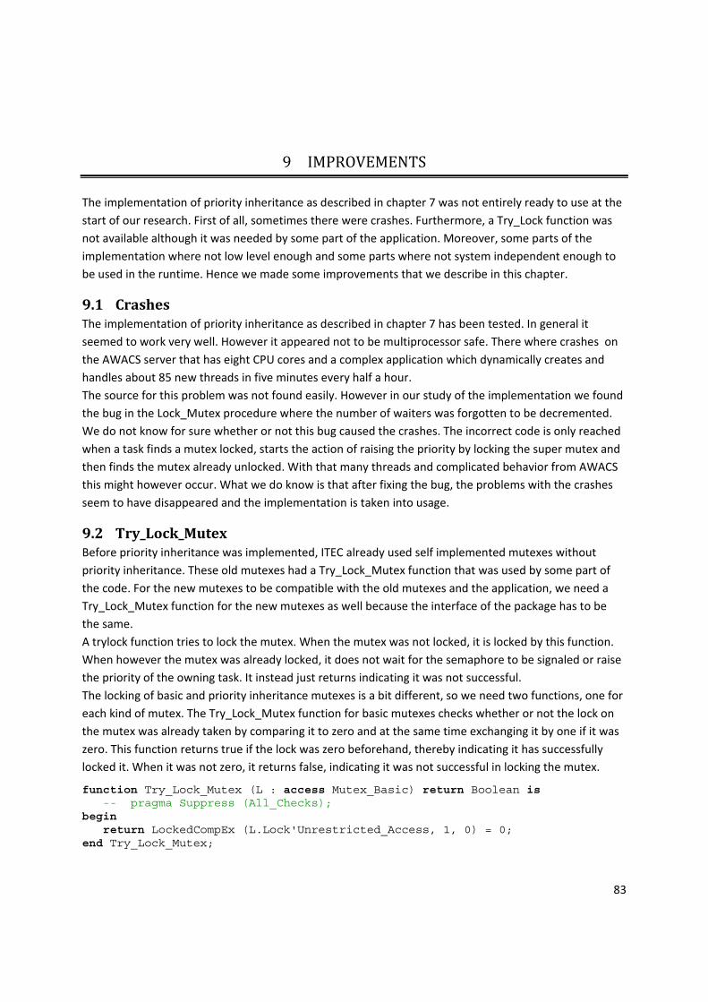
83  

9 IMPROVEMENTS 

The implementation of priority inheritance as described in chapter 7 was not entirely ready to use at the start of our research. First of all, sometimes there were crashes. Furthermore, a Try_Lock function was not available although it was needed by some part of the application. Moreover, some parts of the implementation where not low level enough and some parts where not system independent enough to be used in the runtime. Hence we made some improvements that we describe in this chapter.  

9.1 Crashes The implementation of priority inheritance as described in chapter 7 has been tested. In general it seemed to work very well. However it appeared not to be multiprocessor safe. There where crashes  on the AWACS server that has eight CPU cores and a complex application which dynamically creates and handles about 85 new threads in five minutes every half a hour. The source for this problem was not found easily. However in our study of the implementation we found the bug in the Lock_Mutex procedure where the number of waiters was forgotten to be decremented. We do not know for sure whether or not this bug caused the crashes. The incorrect code is only reached when a task finds a mutex locked, starts the action of raising the priority by locking the super mutex and then finds the mutex already unlocked. With that many threads and complicated behavior from AWACS this might however occur. What we do know is that after fixing the bug, the problems with the crashes seem to have disappeared and the implementation is taken into usage. 

9.2 Try_Lock_Mutex Before priority inheritance was implemented, ITEC already used self implemented mutexes without priority inheritance. These old mutexes had a Try_Lock_Mutex function that was used by some part of the code. For the new mutexes to be compatible with the old mutexes and the application, we need a Try_Lock_Mutex function for the new mutexes as well because the interface of the package has to be the same. A trylock function tries to lock the mutex. When the mutex was not locked, it is locked by this function. When however the mutex was already locked, it does not wait for the semaphore to be signaled or raise the priority of the owning task. It instead just returns indicating it was not successful.  The locking of basic and priority inheritance mutexes is a bit different, so we need two functions, one for each kind of mutex. The Try_Lock_Mutex function for basic mutexes checks whether or not the lock on the mutex was already taken by comparing it to zero and at the same time exchanging it by one if it was zero. This function returns true if the lock was zero beforehand, thereby indicating it has successfully locked it. When it was not zero, it returns false, indicating it was not successful in locking the mutex. 

function Try_Lock_Mutex (L : access Mutex_Basic) return Boolean is -- pragma Suppress (All_Checks); begin return LockedCompEx (L.Lock'Unrestricted_Access, 1, 0) = 0; end Try_Lock_Mutex;

84  

The function for priority inheritance mutexes still has to check whether or not the mutex was already locked by the current task as is done in the Lock_Mutex procedure (7.4.2). Furthermore it cannot exchange the lock simply by one, but has to try to put a pointer to the Task_Data of the current task in it. If the original owner of the mutex was null the function was able to successfully lock the mutex and returns true. If that was not the case it returns false. 

function Try_Lock_Mutex (L : access Mutex_Prio) return Boolean is -- pragma Suppress (All_Checks); P : Ptask_Data := My_Data; Orgowner : Ptask_Data := LockedCompEx (L.Lock'Unrestricted_Access, P, null); begin if Orgowner = P then raise Mutex_Already_Locked; else return Orgowner = null; end if; end Try_Lock_Mutex;

9.3 Task Data In order to use the mutexes as basic locking primitives, they have to be independent of higher structures such as the Task Attributes. So we have to implement another way of keeping track of the task data. We still can use the Task_data type, which is a record, and Ptask_data as a pointer to Task_Data, but not the package Tattr: 

package Tattr is new Ada.Task_Attributes (Task_Data, (Thread => <>, Baseprio => 0, Prio => 0, Raised => (others => (null, 0)), Raised_Last => 0)); use Tattr;

Instead of using the package Ada.Task_attributes, we are going to make a global linked list to keep the Task Data. We call this linked list TaskDataList: 

TaskDataList : aliased Ptask_Data := null;

In the Task_Data type, we add a new component to the record to keep a pointer to the next item in the task data list. 

type Task_Data is record ThreadId : DWORD; Thread : HANDLE; -- Handle to thread Baseprio : Integer; -- Base priority of thread Prio : Unsigned_32; -- Current priority + Gen Raised : Raised_Lock_Array (1 .. 5); Raised_Last : Integer; Next : aliased Ptask_Data; -- next taskdata in linked list end record; pragma Volatile (Task_Data);

Because the TaskDataList is global we want to prevent it from accessing by different tasks at the same time. We cannot use a priority inheritance mutex for this, because we are using the TaskDataList for the priority inheritance mutexes. We can however use a basic mutex to protect the TaskDataList. 

85  

TDLMutex : Mutex := Create_Mutex (Inherit_Prio => False);

In the My_Data function we also have to change some things to work with the task data list. 

function My_Data return Ptask_Data is function To_Ptd is new Ada.Unchecked_Conversion (HANDLE, Ptask_Data); function To_Int is new Ada.Unchecked_Conversion (Ptask_Data, HANDLE); V : HANDLE := TlsGetValue (Tls); begin if V = null then declare R : Ptask_Data := null; begin Lock_Mutex (TDLMutex); Clear_Data; R := new Task_Data'(ThreadId => GetCurrentThreadId, Thread => Create_Thread_Handle, Baseprio => 0, Prio => 0, Raised => (others => (null, 0)), Raised_Last => 0, Next => TaskDataList); TaskDataList := R; Unlock_Mutex (TDLMutex); R.Baseprio := GetThreadPriority (R.Thread); R.Prio := Combine (0, R.Baseprio); if TlsSetValue (Tls, To_Int (R)) = 0 then raise Program_Error; end if; return R; end; else return To_Ptd (V); end if; end My_Data; pragma Inline_Always (My_Data);

First the mutex of the TaskDataList is locked to prevent interference from other tasks. Instead of the following line where the Reference function of the Task Attributes is used. 

R : Ptask_Data := Ptask_Data (Reference);

We now instantiate Ptask_Data with a pointer to a new Task_Data object. 

R := new Task_Data'(ThreadId => GetCurrentThreadId, Thread => Create_Thread_Handle, Baseprio => 0, Prio => 0, Raised => (others => (null, 0)), Raised_Last => 0, Next => TaskDataList);

We put this item in front of the TaskDataList by assigning the original list to “Next”.  And assign the current item to TaskDataList. 

TaskDataList := R;

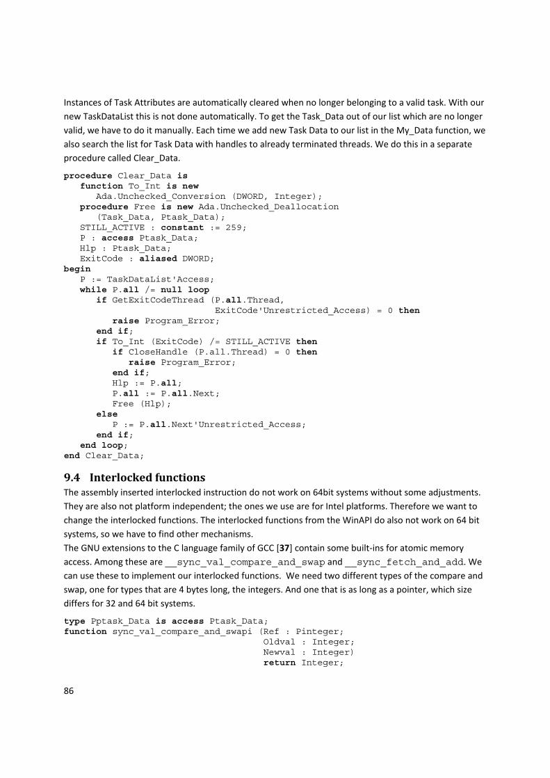
86  

Instances of Task Attributes are automatically cleared when no longer belonging to a valid task. With our new TaskDataList this is not done automatically. To get the Task_Data out of our list which are no longer valid, we have to do it manually. Each time we add new Task Data to our list in the My_Data function, we also search the list for Task Data with handles to already terminated threads. We do this in a separate procedure called Clear_Data. 

procedure Clear_Data is function To_Int is new Ada.Unchecked_Conversion (DWORD, Integer); procedure Free is new Ada.Unchecked_Deallocation (Task_Data, Ptask_Data); STILL_ACTIVE : constant := 259; P : access Ptask_Data; Hlp : Ptask_Data; ExitCode : aliased DWORD; begin P := TaskDataList'Access; while P.all /= null loop if GetExitCodeThread (P.all.Thread, ExitCode'Unrestricted_Access) = 0 then raise Program_Error; end if; if To_Int (ExitCode) /= STILL_ACTIVE then if CloseHandle (P.all.Thread) = 0 then raise Program_Error; end if; Hlp := P.all; P.all := P.all.Next; Free (Hlp); else P := P.all.Next'Unrestricted_Access; end if; end loop; end Clear_Data;

9.4 Interlocked functions The assembly inserted interlocked instruction do not work on 64bit systems without some adjustments. They are also not platform independent; the ones we use are for Intel platforms. Therefore we want to change the interlocked functions. The interlocked functions from the WinAPI do also not work on 64 bit systems, so we have to find other mechanisms.  The GNU extensions to the C language family of GCC [37] contain some built‐ins for atomic memory access. Among these are __sync_val_compare_and_swap and __sync_fetch_and_add. We can use these to implement our interlocked functions.  We need two different types of the compare and swap, one for types that are 4 bytes long, the integers. And one that is as long as a pointer, which size differs for 32 and 64 bit systems.  

type Pptask_Data is access Ptask_Data; function sync_val_compare_and_swapi (Ref : Pinteger; Oldval : Integer; Newval : Integer) return Integer;

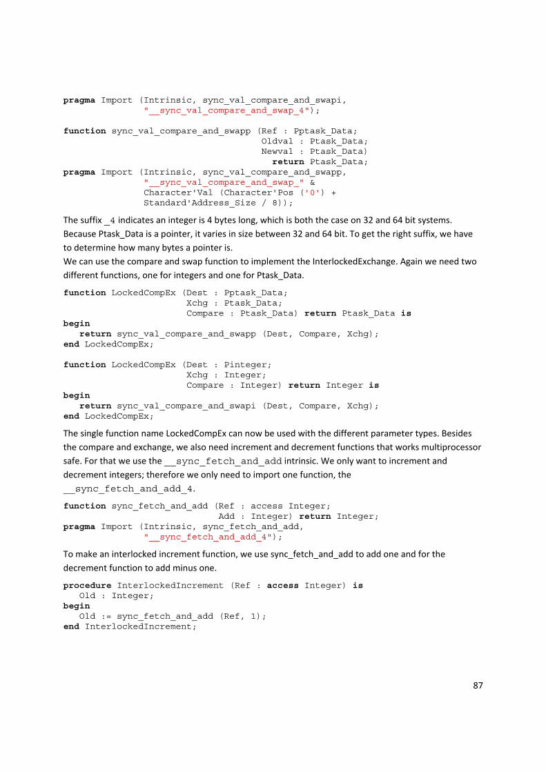
87  

pragma Import (Intrinsic, sync_val_compare_and_swapi, "__sync_val_compare_and_swap_4"); function sync_val_compare_and_swapp (Ref : Pptask_Data; Oldval : Ptask_Data; Newval : Ptask_Data) return Ptask_Data; pragma Import (Intrinsic, sync_val_compare_and_swapp, "__sync_val_compare_and_swap_" & Character'Val (Character'Pos ('0') + Standard'Address_Size / 8));

The suffix _4 indicates an integer is 4 bytes long, which is both the case on 32 and 64 bit systems. Because Ptask_Data is a pointer, it varies in size between 32 and 64 bit. To get the right suffix, we have to determine how many bytes a pointer is. We can use the compare and swap function to implement the InterlockedExchange. Again we need two different functions, one for integers and one for Ptask_Data. 

function LockedCompEx (Dest : Pptask_Data; Xchg : Ptask_Data; Compare : Ptask_Data) return Ptask_Data is begin return sync_val_compare_and_swapp (Dest, Compare, Xchg); end LockedCompEx; function LockedCompEx (Dest : Pinteger; Xchg : Integer; Compare : Integer) return Integer is begin return sync_val_compare_and_swapi (Dest, Compare, Xchg); end LockedCompEx;

The single function name LockedCompEx can now be used with the different parameter types. Besides the compare and exchange, we also need increment and decrement functions that works multiprocessor safe. For that we use the __sync_fetch_and_add intrinsic. We only want to increment and decrement integers; therefore we only need to import one function, the __sync_fetch_and_add_4. 

function sync_fetch_and_add (Ref : access Integer; Add : Integer) return Integer; pragma Import (Intrinsic, sync_fetch_and_add, "__sync_fetch_and_add_4");

To make an interlocked increment function, we use sync_fetch_and_add to add one and for the decrement function to add minus one. 

procedure InterlockedIncrement (Ref : access Integer) is Old : Integer; begin Old := sync_fetch_and_add (Ref, 1); end InterlockedIncrement;

88  

procedure InterlockedDecrement (Ref : access Integer) is Old : Integer; begin Old := sync_fetch_and_add (Ref, -1); end InterlockedDecrement;

To verify our changes of the interlocked functions do not slow down the execution of the mutexes, we measure the execution time of the various interlocked functions. We compare the new interlocked functions with the lock cmpxchgl and lock xaddl assembly insertions that first were used. For comparison we also included the InterlockedCompareExchange and InterlockedIncrement from the Windows API. In Table 5 the results of these measurements can be seen.  

Function  E6300 

lock cmpxchgl  17

__sync_val_compare_and_swap_4  17

InterlockedCompareExchange  29

lock xaddl  15

__sync_fetch_and_add_4  15

InterlockedIncrement  25Table 5: Speed of interlocked functions in ns 

As we can see the assembly insertions and the GCC built‐ins are comparable in speed, where the Windows function are not that fast. So our changes will not slow down the mutexes. 

89  

10 PERFORMANCE MEASUREMENTS 

In this chapter we analyze our improved priority inheritance implementation and perform some measurements on it. In section 10.1 we explain how the mutexes are used. Next we measure the performance of used windows functions (section 10.2). At least the performance of the priority inheritance mutexes (section 10.3) is measured.  

10.1 Collision and Raise count The implementation of the priority inheritance mutexes uses a semaphore for thread signaling. A semaphore cannot be used very fast. However it is only used when a thread encounters a mutex that is already locked.  Furthermore, when priority inheritance occurs, the priority of the thread is raised, which is also not a very fast operation. We have to make sure both these circumstances do not occur very often; else the overall performance will slow down. With increasing usage, the speed becomes more important. Therefore we are going to measure the amount of occurrences of the different circumstances.  When a task wants to lock a mutex which is already locked by another task, there is a collision. When there is a collision and the priority of the task wanting the mutex is higher than the priority of the task having the mutex there is a priority inversion and the priority has to be raised. So there are more collisions than raises and more locks than collisions. We measure each of these things. Therefore we use global variables in the Eln.Mutexesnew package body as we did in section 8.3. 

PrioLockCounter : Integer := 0; CollisionCounter : Integer := 0; InversionCounter : Integer := 0; PrioRaisedCounter : Integer := 0; CountTimes : Integer := 100000;

The purpose of CountTimes is to state when to output the numbers and the time. In this case that is after 100.000 locks. Right at the start of the procedure Lock_Mutex (L : access Mutex_Prio), we printout the counters when necessary. 

if PrioLockCounter mod CountTimes = 0 then Put_Line ("Counted" & PrioLockCounter'Img & " locks," & CollisionCounter'Img & " coll," & InversionCounter'Img & " inv," & PrioRaisedCounter'Img & " raised, on" & Seconds (Clock)'Img & " seconds"); end if; InterlockedIncrement (PrioLockCounter'Unrestricted_Access);

When the task cannot immediately get the lock, because the mutex is already locked, there is a collision, so we increase the collision counter. When there is a collision and the priority of the task wanting the mutex is higher than the priority of the task having the mutex, a priority inversion would occur, so we increase the InversionCounter. The priority has to be raised; this has to be done without interference from other tasks, so a superlock is 

90  

locked. If at this point the mutex is still locked, the priority is actually raised and the PrioRaisedCounter is incremented. In this way, there are more locks than collisions, more collisions than inversions and more inversions than raises. 

InterlockedIncrement (PrioLockCounter'Unrestricted_Access); Orgowner := LockedCompEx (L.Lock'Unrestricted_Access, P, null); if Orgowner = null then return; end if; if Orgowner = P then raise Mutex_Already_Locked; end if; CollisionCounter := CollisionCounter + 1; InterlockedIncrement (L.Waiters'Unrestricted_Access); if To_Prio (Orgowner.Prio) < To_Prio (P.Prio) then InversionCounter := InversionCounter + 1; Lock_Super (P); Orgowner := LockedCompEx (L.Lock'Unrestricted_Access, P, null); if Orgowner = null then Unlock_Super (P); InterlockedDecrement (L.Waiters'Unrestricted_Access); return; end if; if To_Prio (Orgowner.Prio) < To_Prio (P.Prio) then PrioRaisedCounter := PrioRaisedCounter + 1;

Because of the extra instructions in the lock procedure, the mutexes become slower, 124 ns versus 86 ns (measured on the E6300). Because of this, the real number (without the counting) of locks per second might be higher and the number of raises to be lower than the test results shows. The counters are global variables, so they can be accessed by multiple tasks at the same time. To avoid problems with this, we use an InterlockedIncrement to increment the PrioLockCounter. However using interlocked functions further slows down the mutexes and we do not expect the other counters be incremented by multiple tasks at the same time, so we do not use an InterlockedIncrement on these counters. We executed this test on an Adat machine. The machine was running, but was not producing anything. In Table 6 we can see the average locks per second, the raises per second and the percentage of raises compared to the amount of locks. 

  Locks/s  Coll/s  Inv/s  Raises/s Coll/lock  Raise/lock  Inv/Coll  Raise/Coll 

E8400  6014  391  2.7  2.4 6.49% 0.04% 0.67%  0.59%Table 6: Average usage results for Adat 

As we can see, only 0.59 percent of the situation where a mutex finds a mutex already locked, results in a priority raise. In addition in 6.49 percent of the cases there is a collision and it might be needed to use the semaphore. Together with the high amount of locks per second, this supports the point that locking an unoccupied mutex should be performed fast, whether some extra overhead for raising the priority when necessary or using a semaphore is less a problem because it does relatively not occur that often. 

10.2 Speed of Windows functions In section 8.3 we measured how many times a mutex is locked per second, resulting in about 5903 locks per second on the Pentium 4 and about 6074 locks per second for the E8400. As we have seen, on a 

91  

faster computer the number of locks is a bit more per second, but the number of raises is less than half. So additional speed can avoid some priority raises. The longer a mutex object is in use, the higher the chance is that another task needs it in the mean time. So a slow mutex object can introduce more priority inversion. Therefore we want the mutexes to perform as fast as possible. In section 8.4 we measured the duration of the Windows SetPriority function. The test result showed that this function takes relatively long. To know how much time the Windows functions add to the duration of the implementation, we do some performance tests on the functions that are used. The TlsAlloc function allocates an index in the Thread Local Storage (described and used in section 7.4.1) and the TlsFree function frees the index. The TlsSetValue stores a value in the Thread Local Storage for an allocated index value and with the TlsGetValue function the stored value can be retrieved. The SetPriority function is used to change the priority value of a thread. The DuplicateHandle function duplicates an object handle and can convert a pseudo handle of a thread to a real thread handle (handles and objects are described in section 5.4.4; DuplicateHandle is used in section 7.4.1). We measure the times these functions take in the same way we did with measuring the duration of setting the priority in section 8.4. The averages of the concerning Windows functions can be found in Table 7.  

Function  Pentium4 E8400 

TlsAlloc  218 118

TlsFree  936 388

TlsSetValue  8 5

TlsGetValue  6 3

SetPriority  708 249

DuplicateHandle  806 254Table 7: Speed of windows functions in ns 

As we can see, the TlsAlloc and TlsFree functions are not as fast as the TlsSetValue and TlsGetvalue functions. This does not cause much of a problem because only TlsAlloc has to be used once, to get a storage location in the Thread Local Storage for a pointer to the Task Data. The DuplicateHandle function is used once for each task. What is used most is the SetPriority function to change the priority of a thread. This function is taking relatively long, that is why we only want to change the priority if it is necessary.  

10.3 Mutex performance We want to know if the use of priority inheritance in the mutexes does not unnecessary slow down the application. Therefore we want to test the performance of the mutexes. To do this, we compare them with other available synchronization objects. We have some different synchronization objects on different levels. We have the old, newbasic and newprio mutexes implemented by ITEC in Ada, the Protected Objects from Ada, and the Critical Section, Mutex and Semaphore objects from the Windows API. The Rendezvous from Ada is not an object and the projected objects where added to Ada95 because they are much faster than the Rendezvous, so we will not consider the Rendezvous for the comparison.  

92  

For all these synchronization objects we do a lock+unlock operation (ITEC mutexes), enter+leave (Critical Section), wait+release (Mutex and Semaphore) or just enter the object (protected object) to measure the performance of the object. In all this cases the object was not locked yet, which is the case most of the time as we have seen in section 10.1.   

Object  Pentium4  E8400 

OldMutex  80  44

NewMutexBasic  74  38

NewMutexPrio  85  48

Protected Object  88  44

Critical Section  68  26

Mutex object  1657  590

Semaphore Object  938  419Table 8: Speed of synchronization objects in ns 

The test results are not exact measurements, it varies a bit between tests, but we can at least make the relative speed of the synchronization objects visible. As we can see in Table 8, the ITEC new mutexes are comparable in speed to the protected object and critical section. The Windows mutex and semaphore objects take a lot more time. When we look more closely with a couple more measurements, we find (Table 9) that this performance difference is mainly due to the time WaitForSingleObject takes, as opposite to the time LockedcompEx takes which is used in the new mutexes.  

Function  Pentium4  E8400 

WaitForSingleObject  872  308

LockedcompEx  27  8Table 9: Speed in ns 

These test results show that the performance of the mutexes with priority inheritance will not be a problem.  

93  

11 ANALYSIS 

A system that schedules threads based on their priority levels has to make sure the thread with the highest priority is scheduled as fast as possible. The function of a mutex is to protect a shared resource for as long as it takes for the thread holding the resource to finish with it, even with priority inheritance. A high priority task could still be blocked by a low priority task holding a resource [4]. Priority inheritance does not solve all priority inversion problems. Furthermore, priority inheritance is not always the best solution [38]. Especially when it messes up the system of priority levels too much. To solve and avoid problems in the future, we try to get more insight into the priority inversion problem in this chapter. In section 11.1  we check how long mutexes are being kept locked. In section 11.2 we check if the priority system stays more or less intact. 

11.1 Critical section duration We saw in section 10.3 that the mutexes can be locked and unlocked very fast. But we also want to know how long a task holds a mutex, that is, how long a critical section takes. With the priority ceiling protocol, long critical sections would introduce some serious problems, because that means a lot of executing on the highest priority levels, which messes up the priority system very bad. But also without the problems of the priority ceiling protocol, we do not want long critical sections because it would mean more collisions. To test whether or not the critical sections take long, we are going to measure the time between a lock and unlock call of a mutex. If we use the Ada.Calendar.Clock for measuring the lock time of mutexes, it adds about 400 ns for each call to the Clock function. This would add significantly to the duration of locking and unlocking a mutex. Therefore we are going to try to use the HighRes_Time used for scope to measure the lock time, which takes less time. There are about six thousand locks per second; therefore we do not want the duration of each individual mutex lock, which would be unmanageable. We are only really interested in the shortest, longest and average lock time. So that is what we keep count of. 

MinDuration : Duration := Duration'Large; MaxDuration : Duration := 0.0; TotalDuration : Duration := 0.0; Amount : Integer := 0; -- Amount of csdurations added to total CountTimes : Integer := 100000; -- After so many locks it is printed

We add we add a variable Locktime to the mutex to keep track of when the mutex started being locked. 

type Mutex_Prio is new Mutex_Root with record Lock : Ptask_Data; -- Lock flag Waiters : Integer; -- Amount of threads waiting Sem : HANDLE; -- Semaphore for thread signaling LockTime : HighRes_Time; -- Timepoint when the mutex is locked last time end record;

94  

When the mutex is locked, but before the Lock_Mutex procedure returns, we start the clock for the mutex. 

Orgowner := LockedCompEx (L.Lock'Unrestricted_Access, P, null); if Orgowner = null then L.LockTime := Time_Stamp; -- start measuring locktime return; end if;

Also when a task first has to wait for the mutex, but finally can lock it, the LockTime clock has to be started. 

while LockedCompEx (L.Lock'Unrestricted_Access, P, null) /= null loop if WaitForSingleObject (L.Sem) /= WAIT_OBJECT_0 then raise Program_Error; end if; end loop; InterlockedDecrement (L.Waiters'Unrestricted_Access); L.LockTime := Time_Stamp; -- start measuring locktime end Lock_Mutex;

Because we only want to measure the time a task is in its critical section, and not the time it takes to lock and unlock included, we want to stop the time as soon as the task starts unlocking the mutex. 

Orgowner := LockedCompEx (L.Lock'Unrestricted_Access, null, P); Stop := Time_Stamp; Start := L.LockTime;

Because we want as little as possible influence on the time it takes to lock or unlock a mutex, we do all the administration at the end of the unlock function, when the mutex is already unlocked.  

LockDuration := To_Duration (Stop - Start); TotalDuration := TotalDuration + LockDuration; Amount := Amount + 1; if LockDuration < MinDuration then MinDuration := LockDuration; end if; if LockDuration > MaxDuration then MaxDuration := LockDuration; end if;

After a certain amount of mutex usages, we want to output the average, maximum and minimum lock time and we reset these values. 

if Amount mod CountTimes = 0 then Avg := TotalDuration / Amount; Put_Line ("On average locks last" & Avg'Img & ", max was" & MaxDuration'Img & ", min was" & MinDuration'Img); Amount := 0; TotalDuration := 0.0; MinDuration := Duration'Large; MaxDuration := 0.0; end if; end Unlock_Mutex;

95  

Because of these additional instructions, the time it takes for a task to lock or unlock a mutex will take a bit longer. The use of the HighRes_Time still makes the mutexes slower. We test the time of the measuring mutexes with the following function. 

function TestNewMutexMeasure return Duration is use Eln.MutexesMeasure; M : Mutex := Create_Mutex (Inherit_Prio => True); Start : HighRes_Time; Stop : HighRes_Time; begin Start := Time_Stamp; for I in 1 .. Times loop Lock_Mutex (M); Unlock_Mutex (M); end loop; Stop := Time_Stamp; return To_Duration (Stop - Start) / Times * Unit; end TestNewMutexMeasure;

We execute this test on the E6300. This gives the results showed below. The first ten lines are the output of the measuring mutexes; the last line is the result of the above test function. 

On average locks last 0.000000071, max was 0.000016975, min was 0.000000068 On average locks last 0.000000072, max was 0.000012927, min was 0.000000068 On average locks last 0.000000072, max was 0.000010579, min was 0.000000068 On average locks last 0.000000072, max was 0.000009714, min was 0.000000068 On average locks last 0.000000072, max was 0.000009014, min was 0.000000068 On average locks last 0.000000071, max was 0.000011884, min was 0.000000068 On average locks last 0.000000071, max was 0.000011971, min was 0.000000068 On average locks last 0.000000072, max was 0.000013987, min was 0.000000068 On average locks last 0.000000071, max was 0.000011738, min was 0.000000068 On average locks last 0.000000072, max was 0.000010504, min was 0.000000068 MeasureMutexes takes 221.000000000 ns

We see a fluctuation in the maximum time a mutex is locked, although theoretical all times should be the same and minimal because we do not do anything between the lock and unlock of the mutex in this test case. We also see a difference between the times measured by the mutex itself; this is about 72 ns, and the time measured by the surrounding program, that is about 221 ns. This is caused by the administration of the times, after the mutex is unlocked, but before the procedure returns. The most of the added time comes from the To_Duration function, which adds about 65 ns to the unlock function. Because of the longer execution time, the measuring is not convenient for standard incorporation into the mutexes. It would cause more collisions because a task needs to hold the mutex longer. But it is useful to investigate how long critical sections last on average and whether or not there are some mutexes who do take too much processing time while holding the mutex. Next we executed the mutexes with measurements for a real application. This however caused an exception. That is probably caused by the To_Duration function that converts something of the type HighRes_Time to something of the type Duration. This function uses mutexes for its calibration and this circle causes a mutex_already_locked exception. To avoid this problem we are going to use the Ada.Calendar.Clock after all.  The new test provided us with the following results. 

96  

On average locks last 0.000351138, max was 0.519829401, min was-0.000038299 On average locks last 0.000367774, max was 0.071610026, min was-0.000020012 On average locks last 0.000368163, max was 0.066930725, min was-0.000006996 On average locks last 0.000369372, max was 0.069037653, min was-0.000005296 On average locks last 0.000369402, max was 0.071609240, min was-0.000007788

The negative minimum values are caused when the mutex is already locked again by another task, before we calculate the durations. This can probably easily be solved by first saving the start and stop time points before actually unlocking the mutexes. However, the minimum times are not the most interesting aspect. What is more of our concern are the relative high maximum values. The first value of 0.5 seconds is only at startup, but the other maximum values are about 0.07 seconds which is still relatively high, critical sections should not take more than a millisecond. To know what causes this high value we log the thread id of which the critical section is over 0.001 seconds. 

if LockDuration > 0.001 then Put_Line ("Thread " & P.ThreadId'Img& " took " & LockDuration'Img & " seconds"); end if;

This way right at the start of the test results we find the thread id of critical section that took the longest: 

Thread 3232 took 0.519713230 seconds

And after that a couple more times lines that mention the same thread: 

Thread 3232 took 0.064449806 seconds

But the most lines are with thread id 1648: 

Thread 1648 took 0.059413228 seconds

So let’s check what these threads are. When we convert these thread ids to hexadecimal values, we can use the GNU Project Debugger (gdb) to retrieve the corresponding tasks. The decimal value 1648 is 670 hexadecimal. The decimal value 3232 is CA0 hexadecimal. These values we use to acquire the thread information. 

Thread 1 (thread 2008.0xca0): #0 0x7c90eb94 in ntdll!LdrAccessResource () from C:\WINDOWS\system32\ntdll.dll #1 0x7c802532 in WaitForSingleObject () from C:\WINDOWS\system32\kernel32.dll #2 0x00a3e0dc in system.task_primitives.operations.cond_wait () #3 0x00a3e137 in system__task_primitives__operations () #4 0x00a38a2a in system.tasking.stages.vulnerable_complete_master () #5 0x00a38f15 in system.tasking.stages.finalize_global_tasks () #6 0x004037cb in main (argc=Cannot access memory at address 0x0 ) at C:\build\trunk\obj\ada\b~adat.adb:2335 #7 0x00401237 in __mingw_CRTStartup () #8 0x00401288 in mainCRTStartup () Thread 14 (thread 2008.0x670): #0 0x7c90eb94 in ntdll!LdrAccessResource () from C:\WINDOWS\system32\ntdll.dll #1 0x7c802532 in WaitForSingleObject () from C:\WINDOWS\system32\kernel32.dll #2 0x00a3de98 in system.task_primitives.operations.cond_timed_wait () #3 0x00a3dfda in system.task_primitives.operations.timed_sleep () #4 0x00a3b766 in system.tasking.rendezvous.timed_selective_wait ()

97  

#5 0x0067d5cc in heater.omron.e5ck.omron_control_task (<_task>=0x3f704d0) at C:\build\trunk\source\General\Driver\io\heater-omron-e5ck.adb:501 #6 0x00a391d6 in system.tasking.stages.task_wrapper ()

After consulting someone who has knowledge of the different existing tasks and what they are supposed to do, it turns out these are tasks that are doing data transfer. Data transfer usually is not very fast, so it is to be expected these task could hold a mutex locked a bit longer than normally is desirable. However this should not be a problem when the remainder of the system is designed while bearing this in mind. It is useful to regularly check which tasks have long critical section, to make sure everything works as expected. 

11.2 Undesirable raises Priority inheritance is not always the best solution to priority inversion [38] [39], but it can be used easily once it is implemented. However we still have to try to avoid messing up the priorities of tasks too much. We can try to find priority raises which are not necessary or advisable. For example, we do not want the priorities of CPU intensive tasks to be raised to the priority level of the motion planning tasks. That can cause real problems with the continuation of the machine. The program should be designed in such a way that the low level tasks do not lock mutexes also used by the high level tasks. With the ITEC priority level system, it is undesirable when tasks with an initial priority below zero are raised to zero or above (see Figure 27).  

 

2 Motion planning tasks

1 Other important tasks

0 Control tasks 

‐1 CPU intensive tasks

‐2 Visual ITEC tasks

Figure 27: Undesirable priority raises 

We want to know whether or not these undesirable priority raises occur in the current implementation, and want a way to test future implementation against this property. We can log all undesirable priority raises, but we do not always want to check and log them, because it can slow down the execution of the mutexes. Therefore we introduce a flag in the mutex package to indicate whether or not we want to log these priority raises. 

Logging : Boolean := False;

In the Lock_Mutex procedure, if the priority is going to be raised, we check for this flag and then check whether or not there is an undesirable priority raise. If this is the case, we raise an exception and show the ThreadId, original priority and raised priority of the task that was about to do an undesirable priority raise.    

98  

if To_Prio (Orgowner.Prio) < To_Prio (P.Prio) then if Logging then if To_Prio (Orgowner.Prio) < 0 and then To_Prio (P.Prio) >= 0 then declare Priojump : exception; OrgId : DWORD; begin OrgId := GetCurrentThreadId; raise Priojump; exception when E : others => Put_Line ("Priojump " & Exception_Information (E) & "Task " & Orgowner.ThreadId'Img & " is raised from " & To_Prio (Orgowner.Prio)'Img & " to " & To_Prio (P.Prio)'Img); end; end if; end if; Split (P.Prio, Gen, Prio); ...

With the ThreadId and gdb we can retrieve the task that had an undesirable priority raise. We tested this implementation on the E8400 Adat machine, with the expectation to find nothing. However we found one thread rose from a priority of ‐1 to a priority of 2, with the following information. 

Thread 16 (thread 3332.0xba4): #0 0x7c90eb94 in ntdll!LdrAccessResource () from C:\WINDOWS\system32\ntdll.dll #1 0x7c802532 in WaitForSingleObject () from C:\WINDOWS\system32\kernel32.dll #2 0x004fb548 in eln.semaphores.wait_any (obj=0x772b6efe) at C:\build\trunk\source\General\Os_Specific\Eln-Semaphores.adb:94 #3 0x00600336 in cameras.camera_control (<_task>=0x3f5e628) at C:\build\trunk\source\General\Driver\Cameras\Cameras.adb:254 #4 0x00a390b6 in system.tasking.stages.task_wrapper ()

This task has something to do with the camera drivers and should not be raised from a priority of ‐1 to a priority to 2. Why this task is nevertheless raised this high, should be investigated with knowledge of what this task exactly does. Moreover it is useful to regularly check for these undesirable raises, to know if everything is going as expected.  

99  

12 CONCLUSIONS 

In this concluding chapter we cover two things. First the conclusions and answers related to the research questions are presented in section 12.1. Some thoughts and ideas on future research can be found in section 12.2.  

12.1 Answers Now at the end of this thesis we can give the answer and conclusion related to the central question: How can we avoid priority inversion in the systems of ITEC? We do this by first answering our research questions. Question 1: What causes priority inversion in general? In the chapters 2 until 5 we collected a great deal of background information to get a good insight into the problem. As described in the beginning of chapter 6, priority inversion occurs when the scheduling priorities are inverted because of mutual exclusion for data sharing. Question 2: What are solutions to priority inversion problems in literature? Neither in Ada nor in Windows XP priority inversion is prevented. But we found some solutions for unbounded priority inversion in the form of priority inheritance protocols. We made an overview in chapter 6 of the main protocols that could solve the problem. Question 3: How did ITEC implement a solution to priority inversion? The basic priority inheritance protocol was implemented by ITEC; we described this implementation in chapter 7. We have some performance test results in chapter 9, which show the implementation has a good performance. Question 3a: Can the problem with the crashes be solved? While analyzing the implementation, we stumbled upon a bug in the implementation of priority inheritance which could have caused the crashes stated in the problem description. With this bug fixed the implementation as yet works fine. Question 4: Which priority inversion solution would be the best applicable at ITEC? In Chapter 8 we have shown the basic priority inheritance protocol is indeed the best suitable of the protocols in our case.  With the mutex usage analysis of chapter 10, undesirable usage of the mutexes and long critical sections can be tracked down.  Question 5: How can we let the Ada runtime work with priority inheritance? We made a step towards having the central locks of the Ada runtime work with the priority inheritance implementation in chapter 9.  The description of the implementation in chapter 7 together with the improvements for it in chapter 9, make up a good starting point for having the central locks of the Ada runtime work with priority inheritance, with the measurements from chapter 8 as arguments for the protocol choice. The measurements of chapter 9 show that this implementation is satisfactory.  

100  

We now can answer the central question: We can avoid unbounded priority inversion by implementing a priority inheritance protocol, but it is not an easy task, bugs can get in very fast. Moreover priority inheritance does not solve everything, critical sections still should be kept short and undesirable raises avoided. 

12.2 Future research This section we describe some possibilities for future work. 

12.2.1 Ada runtime locks Some work has to be done to get priority inheritance in the Ada runtime library. For getting priority inheritance in the Ada runtime, consulting with AdaCore (the developer and supporter of GNAT) is necessary to retrieve the necessary aspects of a good implementation. Furthermore before we can integrate we have to get a better insight in how the runtime works and is build up. The amount of work it costs to get priority inheritance in the Ada runtime depends on how much the current implementation corresponds to an implementation suitable for integration. In the mean while we have to take into account that priority inheritance is not always a good choice of design for real‐time projects [38] and by making it available in the runtime it could be used without much thought. 

12.2.2 Correctness Before we try to get priority inheritance into the Ada runtime, we it is important to ensure that the implementation is correct. While describing the implementation we already spotted a bug. This shows we cannot be sure there are not more bugs. Because of the complexity of the implementation is not easily shown the implementation is correct. But using the implementation in a real life situation without crashes gives us some confidence it works. However, using this priority inheritance implementation for other applications could bring out incorrectness’s. Therefore a (formal) verification of the implementation might be desirable. For example with the model and verification tool UPPAAL. The difficulty with this is how much details should be included in the model to make sure everything is covered. 

12.2.3 Get more insight into priority inheritance We might like to get more insight in how priority inheritance can be implemented correct. We could investigate other implementations of priority inheritance, for example the priority inheritance of Windows CE or POSIX. How are key problems solved in there? Furthermore we can search for other priority inheritance implementations in Ada. We could look again at the different protocols in more detail. For example, search for existing comparisons of priority inheritance protocols. We also can implement one or more of the other priority inheritance protocols the same way is done with the basic priority inheritance protocol, so a real comparison test can be made. 

12.2.4 Reduce the number of locks Priority inheritance is not always the best solution for priority inversion [38] [39], for example when the difference between priority levels is too high (see section 11.2). We could look at in which situations other solutions are better and why priority inheritance should not be used in those cases. A possible 

101  

solution is using non‐blocking data sharing [40]. With this no priority inversion can occur, because there is no blocking. This may be possible to use in one or more situations as to reduce the number of locks and priority inversions. This could result in the formulation of implementation guidelines when priority inheritance should be used and when it should not be used.  

102  

REFERENCES 

[1] NXP Semiconductors. [Online]. http://www.nxp.com/profile/ 

[2] W. Derks. (2007, Sep.) SPROC‐10. Internal NXP document. 

[3] (2007) Ada Reference Manual. [Online]. http://www.ada‐auth.org/arm.html 

[4] L. Sha, R. Rajkumar, and J. Lehoczky, "Priority Inheritance Protocols: An Approach to Real‐Time Synchronization," IEEE Transactions on Computers, vol. 39, no. 9, Sept 1990. 

[5] A. Burns and A. Wellings, Concurrent and Real‐Time Programming in Ada 2005. Cambridge: Cambridge University Press, 2007. 

[6] W. Stallings, Operating systems, 4th ed. Upper Saddle River, New Jersey: Prentice Hall, 2001. 

[7] M.E. Russinovich and D.A. Solomon, Microsoft® Windows® Internals, Fourth Edition: Microsoft Windows Server™ 2003, Windows XP, and Windows 2000.: Microsoft Press, 2004. 

[8] M. Ben‐Ari, Ada for Software Engineers, 2005th ed. London: Springer‐Verlag, 2009. 

[9] J Miranda. (2002) A Detailed Description of the GNU Ada Run Time. 

[10] H. Hop, M. Tinbergen, and K. ter Haar Romeny, from grains to brains.: Philips Semiconductors Nijmegen, 2000. 

[11] A. Burns, B. Dobbing, and T. Vardanega, "Guide for the use of the Ada Ravenscar Profile in high integrity systems," University of York, Technical Report 2003. 

[12] High Integrity Systems Engineering. [Online]. http://www.cs.york.ac.uk/hise/ 

[13] A. Burns and A. Wellings, Concurrency in ADA, 2nd ed.: Cambridge University Press, 1998. 

[14] Wikipedia. [Online]. www.wikipedia.org 

[15] Microsoft Corporation. (2009, Oktober) Microsoft Developer Network (MSDN). [Online]. http://msdn.microsoft.com/en‐us/default.aspx 

[16] M. Timmerman and J. Monfret, "Windows NT as Real‐Time OS?," Real‐Time Magazine, no. 2, pp. 6‐13, 1997. 

[17] Microsoft Corporation. (1995, June) Real‐Time Systems and Microsoft NT. Technical Article. 

[18] K. Ramamritham and C. Shen, "Using Windows NT for Real‐Time Applications: Experimental Observations and Recommendations," Proceedings of IEEE RTAS'98, June 1998. 

[19] W. Derks. (2000) Ada experience in ITEC. Presentation. 

[20] J. Fuegi and J. Francis, "Lovelace & Babbage and the creation of the 1843 'notes'," Annals of the History of Computing, vol. 25, no. 4, pp. 16 ‐ 26, Oct‐Dec 2003. 

[21] Ada 9X Mapping/Revision Team. (1994) Ada Reference Manual. Online. 

[22] P. Rogers, Programming real‐time with Ada 2005, September 7, 2006. 

[23] (2008, Oct.) GNAT Pro Reference Manual. Document. 

[24] AdaCore. [Online]. www.adacore.com 

103  

[25] O. Dong‐Ik and T.P. Baker, "Optimization of Ada'95 Tasking Constructs," 1994. 

[26] J. Miranda and E. Schonberg. (2004, June) GNAT: The GNU Ada Compiler. document. 

[27] D. A. Wheeler, Ada 95: The Lovelace Tutorial.: Springer‐Verlag, 1997. 

[28] J. Barnes, Programming in Ada 2005.: Addison Wesley, 2006. 

[29] W. Stallings, Operating systems: Internals and Design Principles, 6th ed.: Prentice Hall, 2008. 

[30] R Rajkumar, Synchronization in Real‐Time Systems: A Priority Inheritance Approach. Norwell, United States of America: Kluwer Academic Publishers, 1991. 

[31] J. Richter, Programming Applications for Microsoft Windows, Fourth Edition ed. Redmond, United States of America: Microsoft Press, 1999. 

[32] R. Rajkumar, L. Sha, J.P. Lehoczky, and K. Ramamritham, "An Optimal Priority Inheritance Policy For Synchronization in Real‐Time Systems," in Advances in real‐time systems, S. H. Son, Ed. Upper Saddle River, NJ, USA: Prentice‐Hall, 1995, ch. 11, pp. 249 ‐ 271. 

[33] Windows Programming.: Wikibooks. 

[34] Paolo Gai, "Real Time Operating System design for Multiprocessor system‐on‐a‐chip," RETIS Lab,Scuola Superiore S. Anna, Pisa, PhD Thesis 2005. 

[35] T.P. Baker, "Stack‐Based Scheduling of Realtime Processes," The Journal of Real‐Time Systems, vol. 3, no. 1, pp. 67‐99, March 1991. 

[36] J. Ras and A.M.K. Cheng, "An Evaluation of the Dynamic and Static Multiprocessor Priority Ceiling Protocol and the Multiprocessor Stack Resource Policy in an SMP System," in 15th IEEE Real‐Time and Embedded Technology and Applications Symposium, 2009, pp. 13‐22. 

[37] (2008, October) Using the GNU Compiler Collection (GCC). Manual. 

[38] V Yodaiken, "Against priority inheritance," Finite State Machine Labs (FSMLabs), Technical Report 2004. 

[39] D. Locke. (2002, July) Priority Inheritance: The Real Story. www.linuxdevices.com. 

[40] P. Tsigas and Y. Zhang, "Non‐blocking Data Sharing in Multiprocessor Real‐Time Systems," in Sixth International Conference on Real‐Time Computing Systems and Applications (RTCSA'99), Hong Kong, China, 1999, p. 247. 

[41] M. Ben‐Ari, Ada for Software Engineers. Chichester: John Wiley & Sons, 1998. 

[42] M. Ben‐Ari, Principles of Concurrent and Distributed Programming, Second Edition ed. Harlow, UK: Addison‐Wesley, 2006. 

[43] J.W.S. Liu, Real‐Time Systems. Upper Saddle River, NJ: Prentice Hall, 2000. 

[44] G. Levine, "The control of priority inversion in Ada," ACM SIGAda Ada Letters, vol. VIII, no. 6, pp. 53‐56, Nov./Dec. 1988. 

[45] J.F.A.K. van Benthem, H.P. van Ditmarsch, J. Ketting, and W.P.M. Meyer‐Viol, Logica voor informatici, tweede editie ed. Amsterdam, etc.: Addison‐Wesley, 1994. 

[46] M. Ben‐Ari, Principles of concurrent and distributed programming. New York: Prentice Hall, 1990. 

[47] M. W. Borger and R. Rajkumar, "Implementing Priority Inheritance Algorithms in an Ada Runtime 

104  

System," Software Engineering Institute, Carnegie Mellon University, 1989. 

[48] W. Derks. (2007) Semetric Multi Processing. Presentation. 

[49] D. Cornhil and L. Sha, "Priority Inversion in Ada," ACM SIGAda Ada Letters, vol. VII, no. 7, pp. 30‐32, November/December 1987. 

[50] H.R. Nielson and F. Nielson, Semantics with applications, Rev. ed. ed. Chichester: Wiley, 1999. 

[51] Z. Manna and A. Pnueli, The temporal logic of reactive and concurrent systems. New York; Berlin: Springer‐Verlag, 1992. 

[52] L. Aceto, Reactive systems : modelling, specification and verification. Combridge: Cambridge University Press, 2007. 

[53] Z.Manna and A.Pnueli, Temporal verification of reactive systems : safety. New York: Springer, 1995. 

[54] Priority Inheritance voor Assemblage Machines bij NXP. [Online]. http://www.cs.ru.nl/F.Vaandrager/priority_inheritance.html 

[55] UPPAAL Home. [Online]. http://www.uppaal.com/