Parallel Computing 5 (1987) 165-173 165 North-Holland

Solving PDEs on loosely-coupled parallel processors *

William D. GROPP

Department of Computer Studies, Yale University, New Haven, CT 06520, U.S.A.

Abstract. Partial differential equations (PDEs) account for a large part of scientific computing. As a special domain, they have a number of features which makes their solution on parallel computers particularly attractive. One is the highly-ordered structure of most solution algorithms; there is a regular pattern of memory access. Another is the wide range of solution algorithms from which to choose.

Loosely-coupled parallel processors, using a message passing interprocessor communication mechanism, appear to match the data communication requirements of algorithms for PDEs. However, there are many unanswered questions: What is the best communication topology? How fast should the communication be relative to the floating-point speed? How much memory should each node have? The answers to these questions depend on the algorithms chosen. In this paper, we will look at three different classes of algorithms for PDEs and discuss their implications. From these results, we can make recommendations about the design of the next generation of these parallel computers.

Keywords. Solving PDEs, loosely-coupled parallel processors, Gaussian elimination, iterative methods, complex- ity.

1. Introduction

In this paper we will talk about one particular application area and what it implies about the design of a certain class of parallel computer, the loosely-coupled parallel computer.

In very broad terms, there are two types of parallel computer: the tightly-coupled kind, represented by shared memory, and the loosely-coupled, represented by message passing machines. The essenre of a loosely-coupled computer is a group of processors, each of which contains local memory and a CPU (which may include a vector unit) and is called a node, and communication links to some of the other processors. Over these communication lines messages may be sent.

We can characterize a loosely-coupled parallel computer by the three parameters f , the floating-point speed in seconds per operations, s, the startup time for an IO operation, and r, the transfer rate, both in seconds per operation. It is important to note that, at least in current implementations, s is dominated by software costs (system calls, memory allocation) and thus restricts IO operations on the nodes to not overlap with computation. For similar reasons, s >> r. In current implementations, s >>f, since much more effort has been spent on fast floating-point chips.

The pattern of connections between processors is called the topology of the parallel processor. The most common topologies are the ring, the mesh (usually 2-dimensional), and the binary n-cube.

* This work was supported in part by Office of Naval Research Contract No. N00014-82-K-0184 and Air Force Office of Scientific Research Contract AFOSR-84-0360.

0167-8191/87/$3.50 © 1987, Elsevier Science Publishers B.V. (North-Holland)

166 W.D. Gropp / Solving PDEs on parallel processors

There are many engineering tradeoffs in the design of a loosely-coupled parallel processor. In particular, what are good values of s / f and r/f? How much memory should each node have? What is a good topology? 'Good' in this sense must depend on the choice of problem domain; for this paper, we consider some algorithms used in solving partial differential equations (PDEs). We choose PDEs because they are an important area; indeed, many of the projected uses of parallel computers include PDEs. Further, there appear to be a wide range of PDE algorithms suitable for parallel processing. All of these suggest that PDEs may offer some insights into the design tradeoffs in a parallel processor.

We take a sampling of methods and discuss their what they mean for the various parameters. In Section 2, we discuss explicit methods for time dependent PDEs. In Section 3, we discuss implicit methods in particular 2 methods for solving the systems of linear equations which arise when using implicit methods. Finally, we summarize these results, along with others, and discuss their impact on the design of loosely-coupled parallel processors.

2. Explicit methods

We will assume that any 2 or 3-d grid of size 2 t x 2" x 2 n can be efficiently imbedded in the parallel processor. Such imbeddings are easy on hypercubes; alternately, everything we say here applies equally well to a mesh connected processor of the correct dimension.

2.1. Algorithms

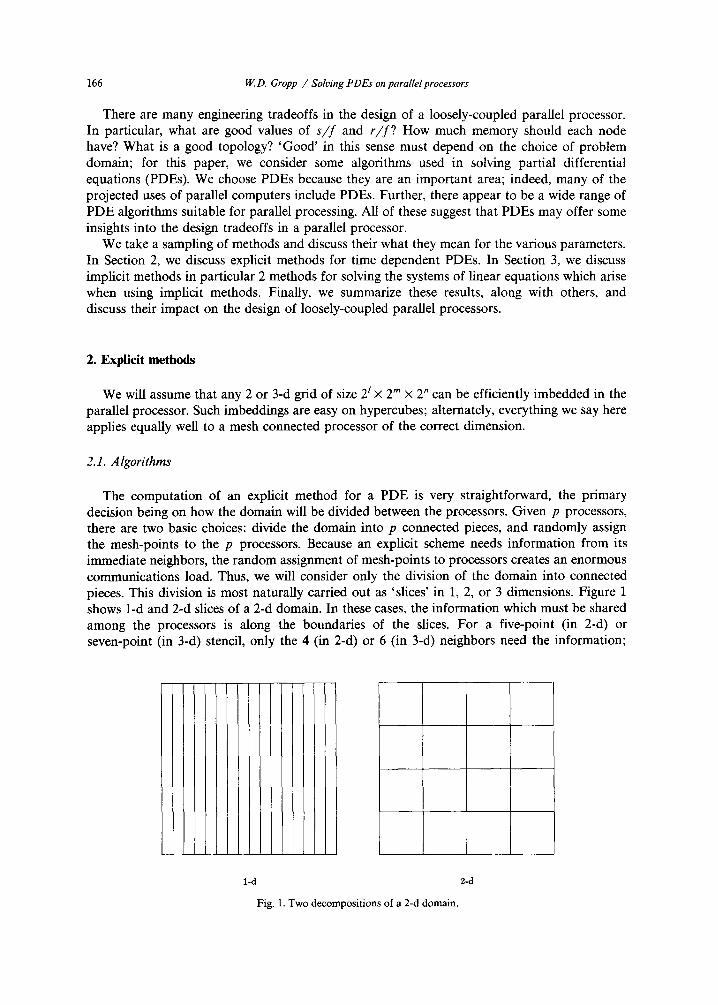
The computation of an explicit method for a PDE is very straightforward, the primary decision being on how the domain will be divided between the processors. Given p processors, there are two basic choices: divide the domain into p connected pieces, and randomly assign the mesh-points to the p processors. Because an explicit scheme needs information from its immediate neighbors, the random assignment of mesh-points to processors creates an enormous communications load. Thus, we will consider only the division of the domain into connected pieces. This division is most naturally carried out as 'slices' in 1, 2, or 3 dimensions. Figure 1 shows 1-d and 2-d slices of a 2-d domain. In these cases, the information which must be shared among the processors is along the boundaries of the slices. For a five-point (in 2-d) or seven-point (in 3-d) stencil, only the 4 (in 2-d) or 6 (in 3-d) neighbors need the information;

1-d 2-d

Fig. 1. Two decompositions of a 2-d domain.

W.D. Gropp / Soloing PDEs on parallel processors 167

with a nine or 27-point stencil, all eight or 26 neighbors must receive the information. Note also that these larger stencils require multiple hops for communication since it is not possible to map the domains onto a hypercube in such a way as to make all of the logical neighbors (in the stencil) neighbors in the hypercube. In each of these cases, we assume that the mesh is mapped onto the hypercube in the manner discussed in [6]. In that mapping, the neighbors in the mesh to the left, right, top, and bottom are adjacent in the hypercube. The diagonal neighbors are two 'hops' away. In 3-d, the situation is similar, except there are 8 neighbors (corners) which are three hops away.

We will consider the cost of computing a step of an explicit PDE on an n × n (in 2-d) and an n × n × n (in 3-d) grid. In each case, it is the length of the boundary of the slice which determines the communication cost. For example, in 2-d where the domain is sliced in one direction, the boundaries between processors are n mesh-points long, so that the effort for one step is

nZf+ 2(s + rn). P

The 2 comes from sending the left internal boundary to the left neighbor and the right internal boundary to the right neighbor. While in principal these operations could go on simultaneously, in practice they require essentially exclusive use of the processor and memory bus. For slices in two directions, there are now either 4 neighbors (for a 5-point stencil) or 8 neighbors (for a 9-point stencil), and the cost becomes

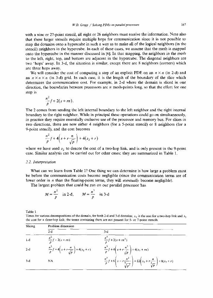
where we have used s 2 to denote the cost of a two-hop link, and is only present in the 9-point case. Similar analysis can be carried out for other cases; they are summarized in Table 1.

2.2. Interpretation

What can we learn from Table 1? One thing we can determine is how large a problem must be before the communication costs become negligible (since the communication terms are of lower order in n than the floating-point terms, they will eventually become negligible).

The largest problem that could be run on our parallel processor has

n 2 n 3

M = - - in2-d, M = - - in3-d P P

Table 1 Times for various decompositions of the domain, for both 2-d and 3-d domains; s 2 is the cost for a two-hop link and s 3 the cost for a three-hop link; the terms containing them are not present for 5- or 7-point stencils

Slicing Problem dimension

2-d 3-d

n 2 1-d - - f + 2 ( s + rn)

P n (5 ) 2-d p f + 4 s + r +4(s2 + r )

3-d NA

n 3 - - f + 2 ( s + rn 2) P

+4( s + r ~ ) +4(s2 + rn) ~f n2

168

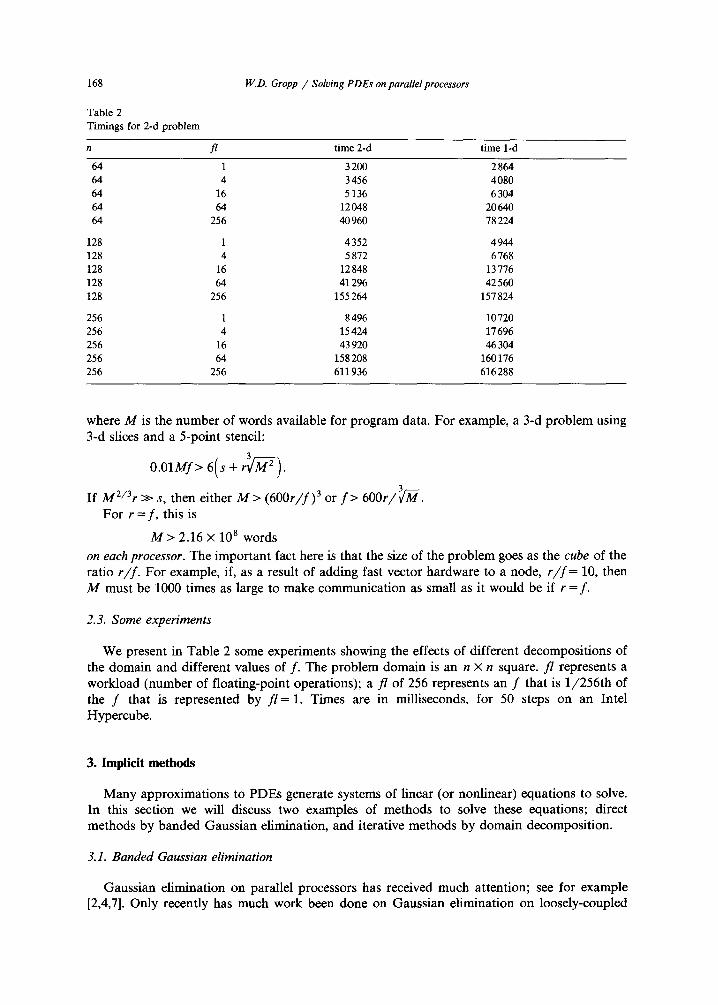
Table 2 Timings for 2-d problem

W.D. Gropp / Soloing PDEs on parallel processors

n fl t ime2-d t i m e l - d

64 1 3 200 2 864 64 4 3456 4080 64 16 5136 6 304 64 64 12 048 20 640 64 256 40 960 78 224

128 1 4 352 4 944 128 4 5 872 6 768 128 16 12 848 13 776 128 64 41296 42 560 128 256 155 264 157 824

256 1 8 496 10 720 256 4 15 424 17 696 256 16 43 920 46 304 256 64 158 208 160176 256 256 611936 616 288

where M is the number of words available for program data. For example, a 3-d problem using 3-d slices and a 5-point stencil:

O.01Mf > 6( s + r3gr-~).

If M2/3r >> s, then either M > (600r/f) 3 or f > 600r/~t-M. For r = f , this is

M > 2.16 X 108 words

on each processor. The important fact here is that the size of the problem goes as the cube of the ratio r / f . For example, if, as a result of adding fast vector hardware to a node, r / f = 10, then M must be 1000 times as large to make communication as small as it would be if r = f .

2.3. Some experiments

We present in Table 2 some experiments showing the effects of different decompositions of the domain and different values of f . The problem domain is an n x n square, f / represents a workload (number of floating-point operations); a f / o f 256 represents an f that is 1/256th of the f that is represented by f / = 1. Times are in milliseconds, for 50 steps on an Intel Hypercube.

3. Implicit methods

Many approximations to PDEs generate systems of linear (or nonlinear) equations to solve. In this section we will discuss two examples of methods to solve these equations; direct methods by banded Gaussian elimination, and iterative methods by domain decomposition.

3.1. Banded Gaussian elimination

Gaussian elimination on parallel processors has received much attention; see for example [2,4,7]. Only recently has much work been done on Gaussian elimination on loosely-coupled

W.D. Gropp / Solving PDEs on parallel processors 169

parallel processors. The fact that s >> r and s >>f can significantly alter the choice of algorithm. In particular, for the Intel Hypercube, the size of s puts a premium on reducing the number of IO starts.

In developing an algorithm for a parallel processor, several questions must be answered. One is "how is the data distributed?". Another is " H o w are the operations ordered?". For full matrices, it is often best to distribute the rows of the matrix in an interleaved fashion. In other words, processor 0 gets rows 1, p + 1, 2p + 1 . . . . . where p is the number of processors. This distribution insures that most of the processors are busy most of the time. The ordering of operations is also important. The easiest to analyze method is for the processors to compute, then to exchange, in a lock-step fashion, pivot rows, then to resume computing. However, a more efficient method is for each processor to run asynchronously in a data-driven way. In this approach, a processor waits until it has received all of the necessary data for it to compute with (in this case, the pivot rows from other processors), then computes and sends information needed by other processors along. The choice of how to send data is also important. In the case of Gaussian elimination, the pivot row must be shared with all other processors. This can be done in many ways. The two most obvious are a global send and a sequential send. In the global send, all the processors cooperate for a brief time to send the data to every processor. On a hypercube, this is an efficient operation, taking roughly log(p)(s + nr) time to send n words. The other approach is to order the processors in a ring and pass the information down the ring. This takes time roughly p(s + nr). From this, it appears that the global send is better. However, while the global send is taking place, all the processors are busy with the send. In the case of the local send, the processors not actually sending can be doing other work. In the case of Gaussian elimination, the local send approach can be shown to be superior.

These considerations lead to the algorithm:

do i = 1, n - 1 if (I have row i)

send to my neighbor else

receive pivot row and forward to my neighbor

use pivot row to eliminate variable i in the rows in this processor

A careful analysis shows that this takes a time of roughly

nm2-------f + 2n(s + mr). P

Unlike the serial case, the back solves can not be neglected since, in terms of s and r, they have the same asymptotic complexity.

3.1.1. Interpretation We can look at how large a problem must be before communication becomes unimportant.

If we consider a 2-d problem so that m = v~- and if we assume that s >> mr, then

The interesting features of this formula are that (1) the size of problem grows faster than linearly in the ratio of IO startup time to

floating-point speed, and (b) as the number of processors used gets larger, the size of the problem must increase.

170

300

0

25O O E

-O

zoO41o

65

t I

W..D. Gropp / Solving PDEs on parallel processors

n = ~ 0 9 6 ' I ' ' I ' ' I

I 4.5

) I , 5 . 0

n - 1 0 2 4 I

I I 5 . 5

I I 6 .0

6O

o

55

50

15

o

~ 1 0 o E

2 3 ~z 5 6

n = 2 5 6 I ' I ' I '

5 i I i 0 3

I , I I 1 2

1 oq ( D r o o c s s o r s )

Fig. 2.

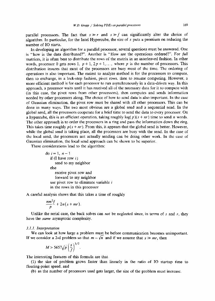
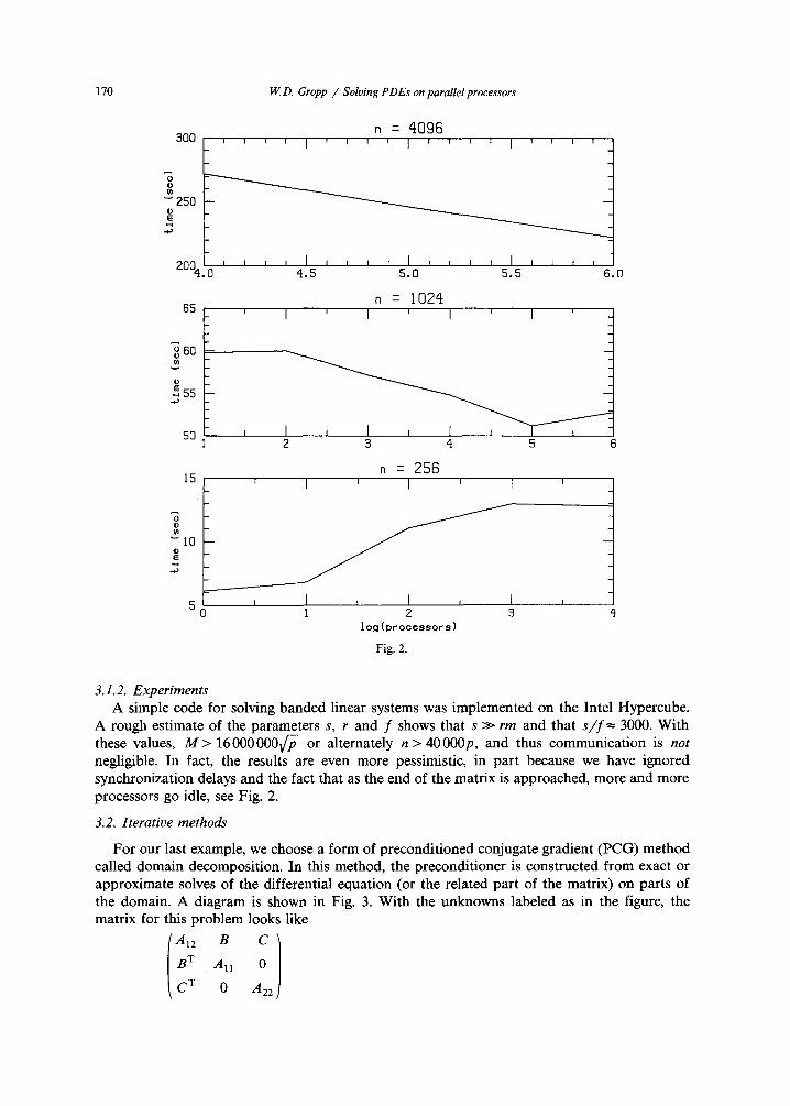
3.1.2. Experiments A simple code for solving banded linear systems was implemented on the Intel Hypercube.

A rough estimate of the parameters s, r and f shows that s >> rm and that s / f = 3000. With these values, M > 16 000 000V/- ~ or alternately n > 40000p, and thus communication is not negligible. In fact, the results are even more pessimistic, in part because we have ignored synchronization delays and the fact that as the end of the matrix is approached, more and more processors go idle, see Fig. 2.

3.2. I terative methods

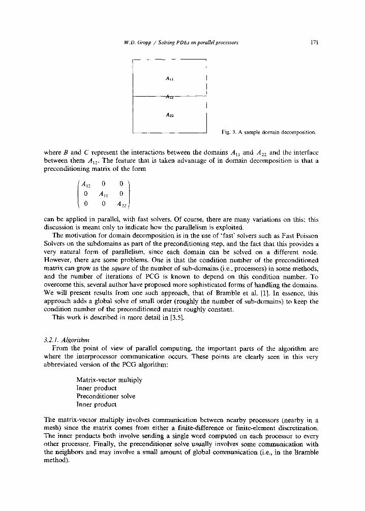
For our last example, we choose a form of preconditioned conjugate gradient (PCG) method called domain decomposition. In this method, the preconditioner is constructed from exact or approximate solves of the differential equation (or the related part of the matrix) on parts of the domain. A diagram is shown in Fig. 3. With the unknowns labeled as in the figure, the matrix for this problem looks like

A12 B C

B T Aal 0

C T 0 A22

W.D. Gropp / Soloing PDEs on parallel processors 171

All

Atz

A22

Fig. 3. A sample domain decomposition.

where B and C represent the interactions between the domains AI~ and A22 and the interface between them A12. The feature that is taken advantage of in domain decomposition is that a preconditioning matrix of the form

All

0 A22

can be applied in parallel, with fast solvers. Of course, there are many variations on this; this discussion is meant only to indicate how the parallelism is exploited.

The motivation for domain decomposition is in the use of 'fast' solvers such as Fast Poisson Solvers on the subdomains as part of the preconditioning step, and the fact that this provides a very natural form of parallelism, since each domain can be solved on a different node. However, there are some problems. One is that the condition number of the preconditioned matrix can grow as the square of the number of sub-domains (i.e., processors) in some methods, and the number of iterations of PCG is known to depend on this condition number. To overcome this, several author have proposed more sophisticated forms of handling the domains. We will present results from one such approach, that of Bramble et al. [1]. In essence, this approach adds a global solve of small order (roughly the number of sub-domains) to keep the condition number of the preconditioned matrix roughly constant.

This work is described in more detail in [3,5].

3.2.1. Algorithm From the point of view of parallel computing, the important parts of the algorithm are

where the interprocessor communication occurs. These points are clearly seen in this very abbreviated version of the PCG algorithm:

Matrix-vector multiply Inner product Preconditioner solve Inner product

The matrix-vector multiply involves communication between nearby processors (nearby in a mesh) since the matrix comes from either a finite-difference or finite-element discretization. The inner products both involve sending a single word computed on each processor to every other processor. Finally, the preconditioner solve usually involves some communication with the neighbors and may involve a small amount of global communication (i.e., in the Bramble method).

172 W..D. Gropp / Solving PDEs on parallel processors

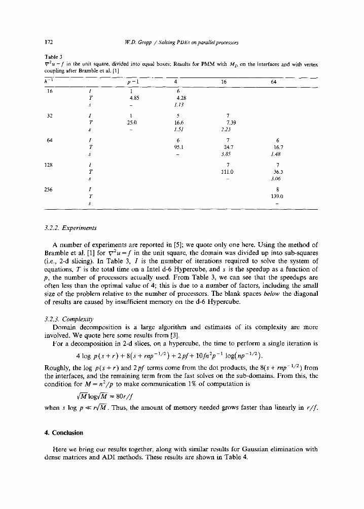
Table 3 VZu = f in the unit square, divided into equal boxes; Results for PMM with M D on the interfaces and with vertex coupling after Bramble et al. [1]

h -1 p =1 4 16 64

16 I 1 6 T 4.85 4.28 s - 1.13

32 1 1 5 7 T 25.0 16.6 7.39 s - 1.51 2.25

64 I 6 7 6 T 95.1 24.7 16.7 s - 3.85 1.48

128 I 7 7 T 111.0 36.3 s - 3.06

256 I 8 T 139.0 S

3.2.2. Experiments

A number of experiments are reported in [5]; we quote only one here. Using the method of Bramble et al. [1] for ~72u = f in the unit square, the domain was divided up into sub-squares (i.e., 2-d slicing). In Table 3, I is the number of iterations required to solve the system of equations, T is the total time on a Intel d-6 Hypercube, and s is the speedup as a function of p, the number of processors actually used. F r o m Table 3, we can see that the speedups are often less than the optimal value of 4; this is due to a number of factors, including the small size of the problem relative to the number of processors. The blank spaces below the diagonal of results are caused by insufficient memory on the d-6 Hypercube.

3.2.3. Complexity Domain decomposi t ion is a large algorithm and estimates of its complexity are more

involved. We quote here some results f rom [3]. For a decomposi t ion in 2-d slices, on a hypercube, the time to perform a single iteration is

4 log p ( s + r ) + 8(s + rnp -1 /2 ) + 2 p f + lOfn2p - l l o g ( n p - 1 / 2 ) .

Roughly, the log p ( s + r ) and 2 p f terms come f rom the dot products, the 8(s + rnp -1 /2) f rom the interfaces, and the remaining term from the fast solves on the sub-domains. F rom this, the condit ion for M = n 2 / p to make communica t ion 1% of computa t ion is

fM-logC'M- ,.~ 8 0 r / f

when s log p << r f M . Thus, the amount of memory needed grows faster than linearly in r / f .

4. Conclusion

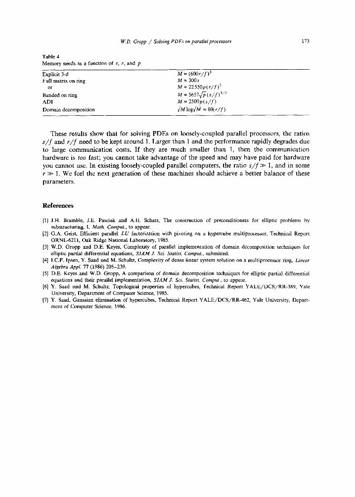
Here we bring our results together, along with similar results for Gaussian elimination with dense matrices and A D I methods. These results are shown in Table 4.

W.D. Gropp /Solv ing PDEs on parallelprocessors 173

Table 4 Memory needs as a function of s, r, and p

Explicit 3-d Full matrix on ring

o r

Banded on ring ADI

Domain decomposition

M = (600r / f ) 3

M = 300 s M = 22550p( r / f ) 2

M = 5657Vrp(s/f) 3/2

M = 2 5 0 0 p ( s / f )

~- log¢ '~ = 80(r/f)

These results show that for solving PDEs on loosely-coupled parallel processors, the ratios s / f and r/ f need to be kept around 1. Larger than I and the performance rapidly degrades due to large communication costs. If they are much smaller than 1, then the communication hardware is too fast; you cannot take advantage of the speed and may have paid for hardware you cannot use. In existing loosely-coupled parallel computers, the ratio s / f >> 1, and in some r >> 1. We feel the next generation of these machines should achieve a better balance of these parameters.

References

[1] J.H. Bramble, J.E. Pasciak and A.H. Schatz, The construction of preconditioners for elliptic problems by substructuring, I, Math. Comput., to appear.

[2] G.A. Geist, Efficient parallel LU factorization with pivoting on a hypercube multiprocessor, Technical Report ORNL-6211, Oak Ridge National Laboratory, 1985.

[3] W.D. Gropp and D.E. Keyes, Complexity of parallel implementation of domain decomposition techniques for elliptic partial differential equations, SIAM J. Sci. Statist. Comput., submitted.

[4] I.C.F. Ipsen, Y. Saad and M. Schultz, Complexity of dense linear system solution on a multiprocessor ring, Linear Algebra Appl. 77 (1986) 205-239.

[5] D.E. Keyes and W.D. Gropp, A comparison of domain decomposition techniques for elliptic partial differential equations and their parallel implementation, S I A M J. Sci. Statist. Comput., to appear.

[6] Y. Saad and M. Schultz, Topological properties of hypercubes, Technical Report YALE/DCS/RR-389, Yale University, Department of Computer Science, 1985.

[7] Y. Saad, Gaussian elimination of hypercubes, Technical Report YALE/DCS/RR-462, Yale University, Depart- ment of Computer Science, 1986.