solving multiple square jigsaw puzzles with missing pieces
TRANSCRIPT
Solving Multiple Square Jigsaw Puzzles with Missing Pieces
Genady PaikinTechnion
Ayellet TalTechnion
Abstract
Jigsaw-puzzle solving is necessary in many applications,including biology, archaeology, and every-day life. Inthis paper we consider the square jigsaw puzzle problem,where the goal is to reconstruct the image from a set ofnon-overlapping, unordered, square puzzle parts. Our keycontribution is a fast, fully-automatic, and general solver,which assumes no prior knowledge about the original im-age. It is general in the sense that it can handle puzzles ofunknown size, with pieces of unknown orientation, and evenpuzzles with missing pieces. Moreover, it can handle all theabove, given pieces from multiple puzzles. Through an ex-tensive evaluation we show that our approach outperformsstate-of-the-art methods on commonly-used datasets.
1. Introduction
Puzzle solving is important in many applications, such asimage editing [4], biology [15] and archaeology [2, 10, 3],to name a few. Though the problem is NP-complete [7, 1],various solutions have been proposed. These are based onshape matching [21, 20, 11, 9] or on a combination of shapematching and color matching [12, 6, 23, 14, 18, 16]. Whenthe parts are square, only color matching is possible [5, 22,17, 8, 19, 13]. The latter is the focus of our work.
The problem is introduced by [5], where a greedy algo-rithm, as well as a benchmark, are proposed. The algorithmdiscussed in [22] improves the results by using a particle fil-ter. Pomeranz et al. [17] introduce the first fully-automaticsquare jigsaw puzzle solver that is based on a greedy placerand on a novel prediction-based dissimilarity. Gallagher [8]generalizes the method to handle parts of unknown orien-tation. Son et al. [13] demonstrate a considerable improve-ment for the case of unknown orientation, by adding ”loopconstraints” to [8]. Rather than pursuing a greedy solver,Sholomon et al. [19] present a genetic algorithm that is ableto solve large puzzles.
Our work is inspired by [17]. However, it takes the nextstep and not only improves upon state-of-the-art results, but
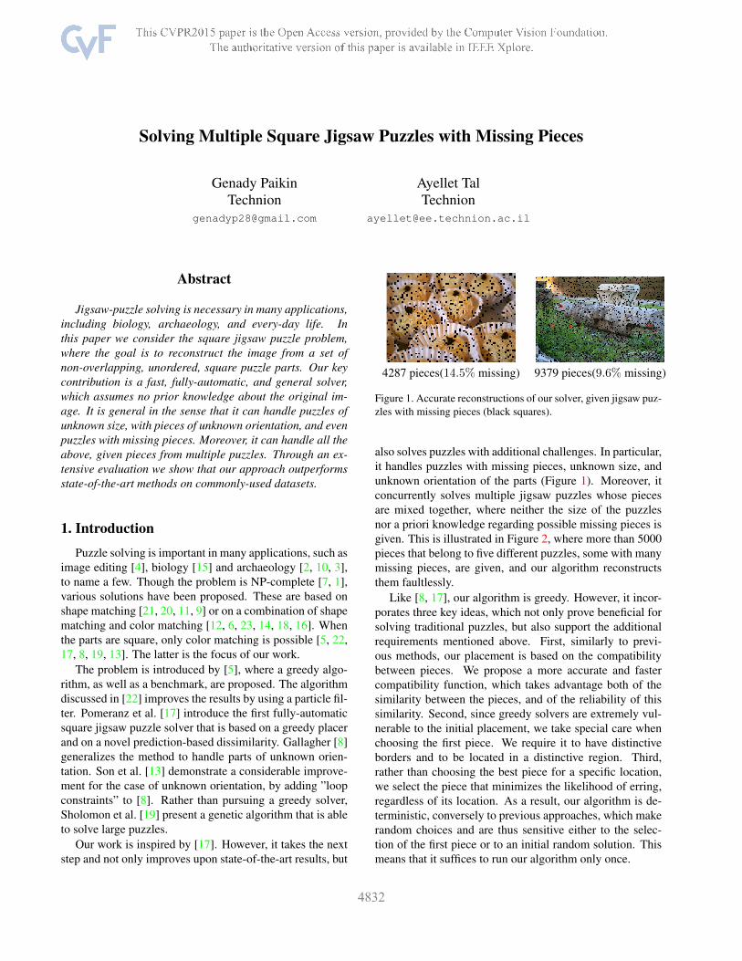
4287 pieces(14.5% missing) 9379 pieces(9.6% missing)
Figure 1. Accurate reconstructions of our solver, given jigsaw puz-zles with missing pieces (black squares).
also solves puzzles with additional challenges. In particular,it handles puzzles with missing pieces, unknown size, andunknown orientation of the parts (Figure 1). Moreover, itconcurrently solves multiple jigsaw puzzles whose piecesare mixed together, where neither the size of the puzzlesnor a priori knowledge regarding possible missing pieces isgiven. This is illustrated in Figure 2, where more than 5000pieces that belong to five different puzzles, some with manymissing pieces, are given, and our algorithm reconstructsthem faultlessly.
Like [8, 17], our algorithm is greedy. However, it incor-porates three key ideas, which not only prove beneficial forsolving traditional puzzles, but also support the additionalrequirements mentioned above. First, similarly to previ-ous methods, our placement is based on the compatibilitybetween pieces. We propose a more accurate and fastercompatibility function, which takes advantage both of thesimilarity between the pieces, and of the reliability of thissimilarity. Second, since greedy solvers are extremely vul-nerable to the initial placement, we take special care whenchoosing the first piece. We require it to have distinctiveborders and to be located in a distinctive region. Third,rather than choosing the best piece for a specific location,we select the piece that minimizes the likelihood of erring,regardless of its location. As a result, our algorithm is de-terministic, conversely to previous approaches, which makerandom choices and are thus sensitive either to the selec-tion of the first piece or to an initial random solution. Thismeans that it suffices to run our algorithm only once.
1
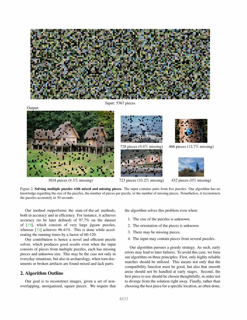
Input: 5367 piecesOutput:
728 pieces (9.6% missing) 466 pieces (13.7% missing)
3018 pieces (8.5% missing) 723 pieces (10.2% missing) 432 pieces (0% missing)
Figure 2. Solving multiple puzzles with mixed and missing pieces. The input contains parts from five puzzles. Our algorithm has noknowledge regarding the size of the puzzles, the number of pieces per puzzle, or the number of missing pieces. Nonetheless, it reconstructsthe puzzles accurately in 30 seconds.
Our method outperforms the state-of-the-art methods,both in accuracy and in efficiency. For instance, it achievesaccuracy (to be later defined) of 97.7% on the datasetof [19], which consists of very large jigsaw puzzles,whereas [19] achieves 96.41%. This is done while accel-erating the running times by a factor of 60-120.
Our contribution is hence a novel and efficient puzzlesolver, which produces good results even when the inputconsists of pieces from multiple puzzles, each has missingpieces and unknown size. This may be the case not only ineveryday situations, but also in archaeology, when torn doc-uments or broken artifacts are found mixed and lack parts.
2. Algorithm OutlineOur goal is to reconstruct images, given a set of non-
overlapping, unorganized, square pieces. We require that
the algorithm solves this problem even when:
1. The size of the puzzles is unknown.
2. The orientation of the pieces is unknown.
3. There may be missing pieces.
4. The input may contain pieces from several puzzles.
Our algorithm pursues a greedy strategy. As such, earlyerrors may lead to later failures. To avoid this case, we baseour algorithm on three principles: First, only highly reliablematches should be utilized. This means not only that thecompatibility function must be good, but also that smoothareas should not be handled at early stages. Second, thefirst piece to use should be chosen thoughtfully, in order notto diverge from the solution right away. Finally, rather thanchoosing the best piece for a specific location, as often done,
we prefer to select the most distinctive piece, one that min-imizes the likelihood of erring, regardless of its location.
Our algorithm proceeds in three steps: calculating thecompatibility between the pieces, finding the best piece tostart with, and assembly. The first step (Section 3) evaluatesthe compatibility between every pair of pieces. We note thatthe dissimilarity between the parts is not sufficiently infor-mative. Hence, we also use the reliability of a match. Thisleaves smooth area to the end of the assembly and assists inhandling puzzles with missing pieces.
The second step (Section 4) finds the best piece to startwith. The key idea is to select a piece that is not only dis-tinctive, but also belongs to a distinctive region. This leadsto high confidence in the first assemblies.
The last step places the pieces (Section 5). This is doneby iteratively selecting a piece to be assembled, utilizing thecompatibility function from Step 1 and the concept of ”bestbuddy” [17]. A guiding principle is that the absolute loca-tion of a piece is determined only when all the pieces foundtheir neighbors. This is very similar to the way people solvepuzzles, constructing different portions of the puzzles sep-arately, before composing them together. This not only letsus solve puzzles of unknown size and unknown orientation,but interestingly, also handles puzzles with missing pieces.
The only input of the algorithm is the number of puz-zles that need to be solved out of the mixed pieces. Duringthe assembly, when all the pieces have low compatibilityvalues, the algorithm starts a new puzzle (up to the givennumber of puzzles), by selecting a new initial piece.
3. The Compatibility MetricA good compatibility metric is a fundamental compo-
nent of every jigsaw puzzle solver. Given two pieces pi, pj ,the compatibility function C(pi, pj , r) predicts the likeli-hood that pi and pj are neighbors in the spatial relation r,r ∈ {up, down, left, right}. We compute the compati-bility function in two steps. First, a dissimilarity betweenevery pair of pieces is calculated. Then, we compute theconfidence in this dissimilarity.
3.1. The Dissimilarity Between Pieces
Various dissimilarity measures have been proposed inthe literature, including L2 [5, 19] and MGC (Mahalanobisgradient compatibility) [8]. Our work is inspired by that ofPomeranz et al. [17], which introduces a prediction-baseddissimilarity. We modify it, as explained below, to makeit not only simpler and faster to compute, but also performbetter, as demonstrated in Figure 3.
Briefly, in [17] backward-difference estimation is em-ployed. It uses the last two pixels in each row (column)near the boundary, from which prediction of the first pixelin the adjacent piece is obtained. The dissimilarity measurebetween pixels in two pieces uses the Lq
p norm, as follows,
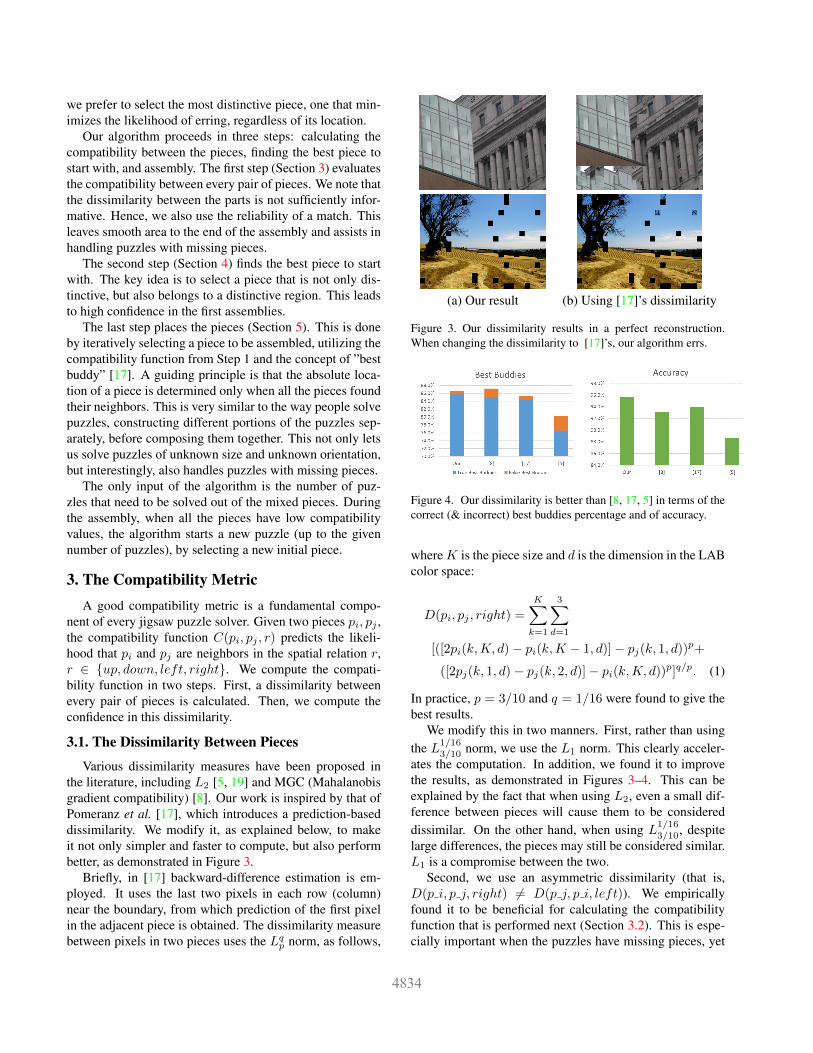
(a) Our result (b) Using [17]’s dissimilarity
Figure 3. Our dissimilarity results in a perfect reconstruction.When changing the dissimilarity to [17]’s, our algorithm errs.
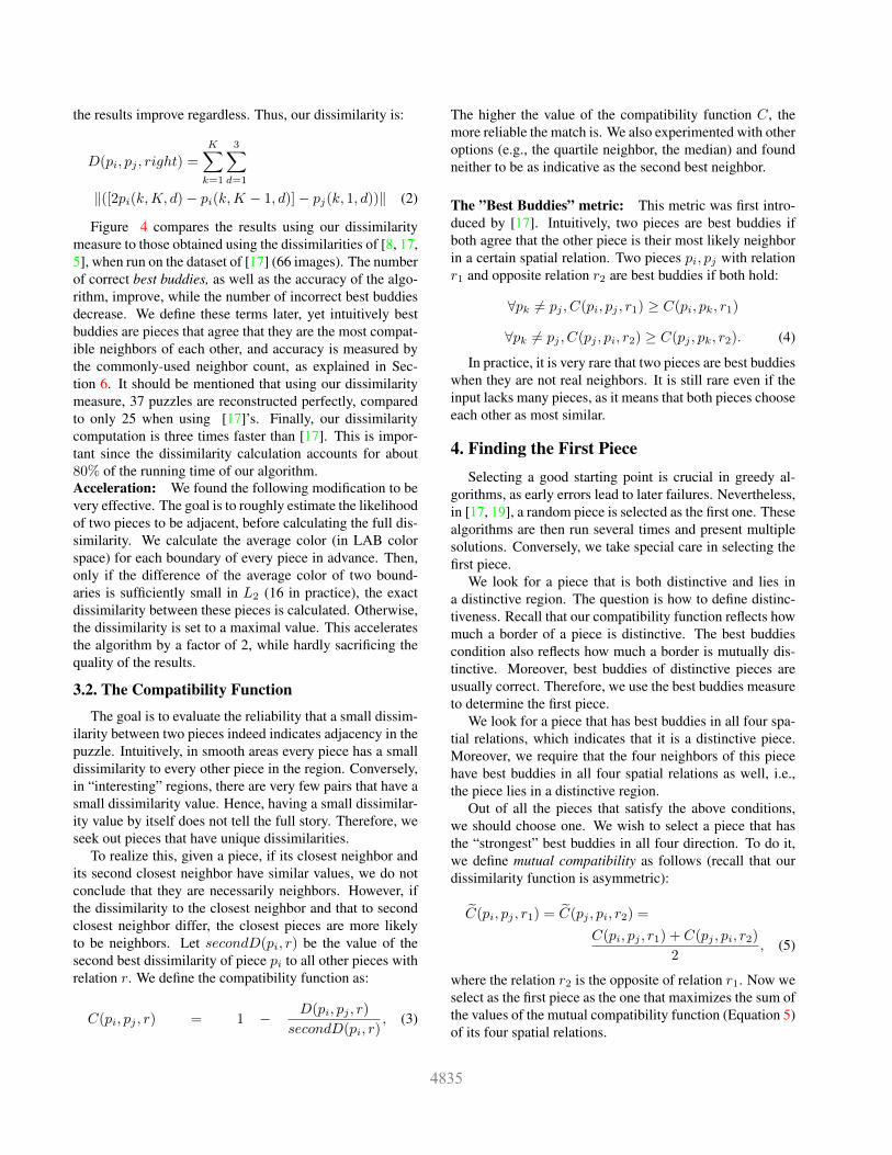
Figure 4. Our dissimilarity is better than [8, 17, 5] in terms of thecorrect (& incorrect) best buddies percentage and of accuracy.
where K is the piece size and d is the dimension in the LABcolor space:
D(pi, pj , right) =
K∑k=1
3∑d=1
[([2pi(k,K, d)− pi(k,K − 1, d)]− pj(k, 1, d))p+
([2pj(k, 1, d)− pj(k, 2, d)]− pi(k,K, d))p]q/p. (1)
In practice, p = 3/10 and q = 1/16 were found to give thebest results.
We modify this in two manners. First, rather than usingthe L
1/163/10 norm, we use the L1 norm. This clearly acceler-
ates the computation. In addition, we found it to improvethe results, as demonstrated in Figures 3–4. This can beexplained by the fact that when using L2, even a small dif-ference between pieces will cause them to be considereddissimilar. On the other hand, when using L
1/163/10, despite
large differences, the pieces may still be considered similar.L1 is a compromise between the two.
Second, we use an asymmetric dissimilarity (that is,D(p i, p j, right) 6= D(p j, p i, left)). We empiricallyfound it to be beneficial for calculating the compatibilityfunction that is performed next (Section 3.2). This is espe-cially important when the puzzles have missing pieces, yet
the results improve regardless. Thus, our dissimilarity is:
D(pi, pj , right) =
K∑k=1
3∑d=1
‖([2pi(k,K, d)− pi(k,K − 1, d)]− pj(k, 1, d))‖ (2)
Figure 4 compares the results using our dissimilaritymeasure to those obtained using the dissimilarities of [8, 17,5], when run on the dataset of [17] (66 images). The numberof correct best buddies, as well as the accuracy of the algo-rithm, improve, while the number of incorrect best buddiesdecrease. We define these terms later, yet intuitively bestbuddies are pieces that agree that they are the most compat-ible neighbors of each other, and accuracy is measured bythe commonly-used neighbor count, as explained in Sec-tion 6. It should be mentioned that using our dissimilaritymeasure, 37 puzzles are reconstructed perfectly, comparedto only 25 when using [17]’s. Finally, our dissimilaritycomputation is three times faster than [17]. This is impor-tant since the dissimilarity calculation accounts for about80% of the running time of our algorithm.Acceleration: We found the following modification to bevery effective. The goal is to roughly estimate the likelihoodof two pieces to be adjacent, before calculating the full dis-similarity. We calculate the average color (in LAB colorspace) for each boundary of every piece in advance. Then,only if the difference of the average color of two bound-aries is sufficiently small in L2 (16 in practice), the exactdissimilarity between these pieces is calculated. Otherwise,the dissimilarity is set to a maximal value. This acceleratesthe algorithm by a factor of 2, while hardly sacrificing thequality of the results.
3.2. The Compatibility Function
The goal is to evaluate the reliability that a small dissim-ilarity between two pieces indeed indicates adjacency in thepuzzle. Intuitively, in smooth areas every piece has a smalldissimilarity to every other piece in the region. Conversely,in “interesting” regions, there are very few pairs that have asmall dissimilarity value. Hence, having a small dissimilar-ity value by itself does not tell the full story. Therefore, weseek out pieces that have unique dissimilarities.
To realize this, given a piece, if its closest neighbor andits second closest neighbor have similar values, we do notconclude that they are necessarily neighbors. However, ifthe dissimilarity to the closest neighbor and that to secondclosest neighbor differ, the closest pieces are more likelyto be neighbors. Let secondD(pi, r) be the value of thesecond best dissimilarity of piece pi to all other pieces withrelation r. We define the compatibility function as:
C(pi, pj , r) = 1 − D(pi, pj , r)
secondD(pi, r), (3)
The higher the value of the compatibility function C, themore reliable the match is. We also experimented with otheroptions (e.g., the quartile neighbor, the median) and foundneither to be as indicative as the second best neighbor.
The ”Best Buddies” metric: This metric was first intro-duced by [17]. Intuitively, two pieces are best buddies ifboth agree that the other piece is their most likely neighborin a certain spatial relation. Two pieces pi, pj with relationr1 and opposite relation r2 are best buddies if both hold:
∀pk 6= pj , C(pi, pj , r1) ≥ C(pi, pk, r1)
∀pk 6= pj , C(pj , pi, r2) ≥ C(pj , pk, r2). (4)
In practice, it is very rare that two pieces are best buddieswhen they are not real neighbors. It is still rare even if theinput lacks many pieces, as it means that both pieces chooseeach other as most similar.
4. Finding the First PieceSelecting a good starting point is crucial in greedy al-
gorithms, as early errors lead to later failures. Nevertheless,in [17, 19], a random piece is selected as the first one. Thesealgorithms are then run several times and present multiplesolutions. Conversely, we take special care in selecting thefirst piece.
We look for a piece that is both distinctive and lies ina distinctive region. The question is how to define distinc-tiveness. Recall that our compatibility function reflects howmuch a border of a piece is distinctive. The best buddiescondition also reflects how much a border is mutually dis-tinctive. Moreover, best buddies of distinctive pieces areusually correct. Therefore, we use the best buddies measureto determine the first piece.
We look for a piece that has best buddies in all four spa-tial relations, which indicates that it is a distinctive piece.Moreover, we require that the four neighbors of this piecehave best buddies in all four spatial relations as well, i.e.,the piece lies in a distinctive region.
Out of all the pieces that satisfy the above conditions,we should choose one. We wish to select a piece that hasthe “strongest” best buddies in all four direction. To do it,we define mutual compatibility as follows (recall that ourdissimilarity function is asymmetric):
C̃(pi, pj , r1) = C̃(pj , pi, r2) =
C(pi, pj , r1) + C(pj , pi, r2)
2, (5)
where the relation r2 is the opposite of relation r1. Now weselect as the first piece as the one that maximizes the sum ofthe values of the mutual compatibility function (Equation 5)of its four spatial relations.
5. Greedy Placement
Our algorithm’s final step assembles the pieces. This isdone without prior knowledge regarding missing pieces orthe size of the puzzle. Our placer (Algorithm 1) is greedyand relies on our mutual compatibility function C̃ (Equa-tion 5). It maintains a pool of candidate pieces to be placed.It iterates on placing a piece from this pool and then addingcandidates to it. We elaborate below.
Algorithm 1 Placer1: While there are unplaced pieces2: if the pool is not empty3: Extract the best candidate from the pool4: else5: Recalculate the compatibility function6: Find the best neighbors (not best buddies)7: Place the above best piece8: Add the best buddies of this piece to the pool
The selected piece is the one having the highest mutualcompatibility function among the pieces in the pool. If thecandidates’ pool is empty, but the jigsaw puzzle is not yetsolved, the compatibility function is recalculated. This isperformed by considering only the pieces that have not yetbeen placed. Then, the next piece to be placed is selectedaccording to the mutual compatibility function, regardlessof whether it is a best buddy of an already-placed piece. Itis placed, as before, next to an already-placed piece. Then,the best buddies (at the various directions) of the newly-place piece are added to the pool.
The placement is performed without determining the ex-act location. That is to say, a piece is placed in a locationthat is relative to other pieces and not in a specific abso-lute location. However, if the algorithm gets as input thepuzzle’s dimensions, the placement is limited to the givenheight and width.
The algorithm performs well even if the puzzle lackspieces. This is because the algorithm never searches for thebest piece for a specific place, as previously done. Thus,holes need not be filled. Moreover, only highly reliableneighbors are selected—those having distinctive borders.This makes the likelihood that a chosen piece is not a realneighbor low.
Similarly, when the algorithm is required to solve mixedpuzzles, the only adjustment needed is the following. Whenall the placed pieces have a relatively small value of mutualcompatibility to all the unplaced pieces (0.5 in our experi-ments), a new puzzle is started. In this case, the candidates’pool is cleared, and a new first piece is selected. This pro-cess repeats until the given number of puzzles is reached.The placement proceeds simultaneity on all the partial solu-tions, until there are no remaining pieces.
6. ResultsOur puzzle solver is applied to the datasets of [5, 17, 19].
These contain three sets, each of 20 images, with 432 [5],540 and 805 pieces [17] respectively, two sets of medium-size puzzles, each containing 3 images with 2360 and 3300pieces [17], and three sets of large puzzles, each containing20 images with 5015, 10375 and 22834 pieces [19] respec-tively. We first quantitatively compare our results to those ofprevious works when applied to the traditional jigsaw puz-zle problem, where the size of puzzle is known and there areno missing pieces. Then we test our algorithm qualitatively(as there is no previous work) on additional cases, includingpuzzles of unknown size, puzzles with missing pieces, andmixed puzzles.
Evaluation when applied to the classical problem: Ta-ble 1 reports the results, averaged per set, using the threecommon measures. The average neighbor measure [5] isthe standard measure, which considers the fraction of thecorrect pairwise adjacencies. It shows the average resulton [5, 17, 19] datasets and compares the results to thoseof the state-of-the-art algorithms of [13, 17, 19]. It can beseen that our algorithm is competitive with [13, 19] andoutperforms [17]. However, it should be noted that whileour result is deterministic, [17, 19] run their algorithms 10times and report the results, in particular the best one.
The direct measure [5] considers the fraction of thepieces in the assembled puzzle that are in their correct ab-solute position. Generally, this measure is considered to beless accurate and less meaningful due to its inability to copewith slightly shifted puzzle. Our algorithm performs betterthan [17, 19] and is comparable to [13].
Finally, the perfect columns indicate the number of puz-zles for which the algorithms produced perfect reconstruc-tions of the puzzle. Our algorithm has a clear advantage inthis regard.
Table 2 reports the results when applied to the datasetof [19] that contains large puzzles. As only the algorithmof [19] was applied to this dataset, we compare only to it. Itcan be seen that our algorithm is beneficial for large puzzleswhen considering each of the measures.
Our algorithm is advantageous also in terms of runningtimes. Table 3 compares our running times to those reportedin [19], which was applied to large puzzles. Our algorithmis considerably faster for all puzzle sizes.
As another comparison, it is reported in [13] that the al-gorithm solves a 9801-piece jigsaw puzzle with unknownorientation in 25.6 hours. Our algorithm solves a 10375-pieces puzzle with unknown orientation in 2 minutes.
Our algorithm was implemented in Java and ran on anIntel i7 processor with 32GB RAM (all recent work ran onsimilar PCs). It should be noted that as our algorithm neednot be adapted in order to solve puzzles with missing pieces,
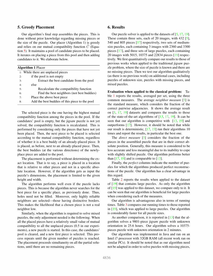
neighbor direct perfect# of pieces Our [13] [19] [17] Our [13] [19] [17] Our [13] [19] [17]432 95.82% 95.5% 96.16% 94.25% 96.16% 95.6% 86.19% 90.95% 13 13 9 13540 96.1% 95.2% 95.96% 90.9% 93.22% 92.2% 92.75% 83.45% 13 - 8 9805 95.09% 94.9% 96.26% 89.7% 92.47% 93.1% 94.67% 80.25% 9 - 10 72360 96.26% 96.4% 88.86% 84.67% 94.01% 94.4% 85.73% 33.4% 1 - 1 13300 95.29% 96.4% 92.76% 85% 90.69% 92% 89.92% 80.67% 1 - 1 1Overall 95.68% 95.31% 95.64% 91% 93.8% 93.59% 90.9% 82.35% 37 - 29 31
Table 1. Comparisons of our results to the state-of-the-art. Our algorithm outperforms state-of-the-art algorithms in all the commonly-used measures. (’-’ mean that the results are not reported.) The comparison is made to the best-out-of-10 result of [17, 19]. Whenconsidering the worst or the average case, their results are slightly worse.
neighbor direct perfectbest worst best worst best worst
# of pieces Our [19] Our [19] Our [19]5015 96.43% 95.25% 94.87% 95.79% 94.78% 90.76% 12 11 710375 98.94% 98.47% 98.2 98.63% 97.69% 96.08% 8 6 522755 97.74% 96.28% 96.17 96.78% 92.02% 91.74% 3 4 4Overall 97.7% 96.67% 96.41 97.07% 94.83% 92.77% 23 21 16
Table 2. Comparisons of our results to the state-of-the-art. Our algorithm outperforms the best solutions of [19] considering the commonmeasures on the dataset of [19], which contains large jigsaw puzzles. The other methods do not provide results on this dataset.
# of # of [19] Our Ratiopieces images432 20 48.73 [sec] 0.59 [sec] 82.59540 20 64.06 [sec] 0.92 [sec] 69.63805 20 116.18 [sec] 1.52 [sec] 76.432360 3 17.6 [min] 8.73 [sec] 120.963300 3 30.24 [min] 14.99 [sec] 121.045015 20 61.06 [min] 28.77 [sec] 127.3410375 20 3.21 [hr] 2.06 [min] 93.522755 20 13.19 [hr] 14.75 [min] 60.7
Table 3. Comparison of the average running times. Our algo-rithm is 60-127 times faster.
the running times are similar in this case as well.
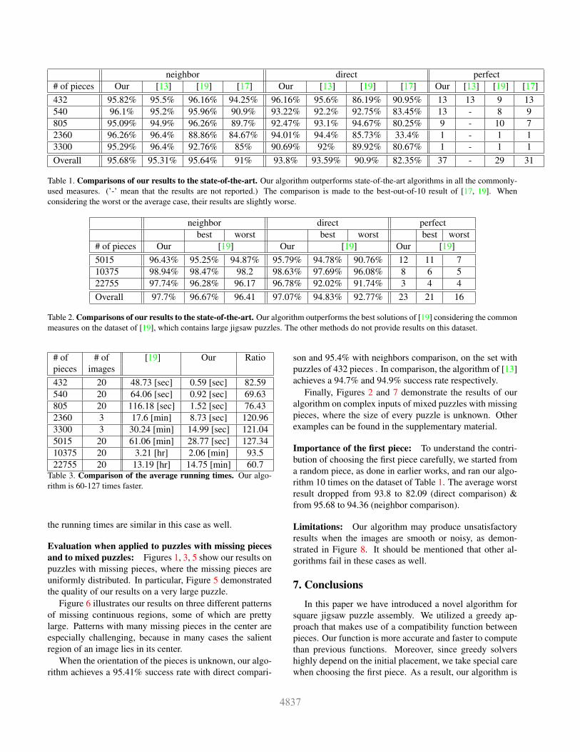
Evaluation when applied to puzzles with missing piecesand to mixed puzzles: Figures 1, 3, 5 show our results onpuzzles with missing pieces, where the missing pieces areuniformly distributed. In particular, Figure 5 demonstratedthe quality of our results on a very large puzzle.
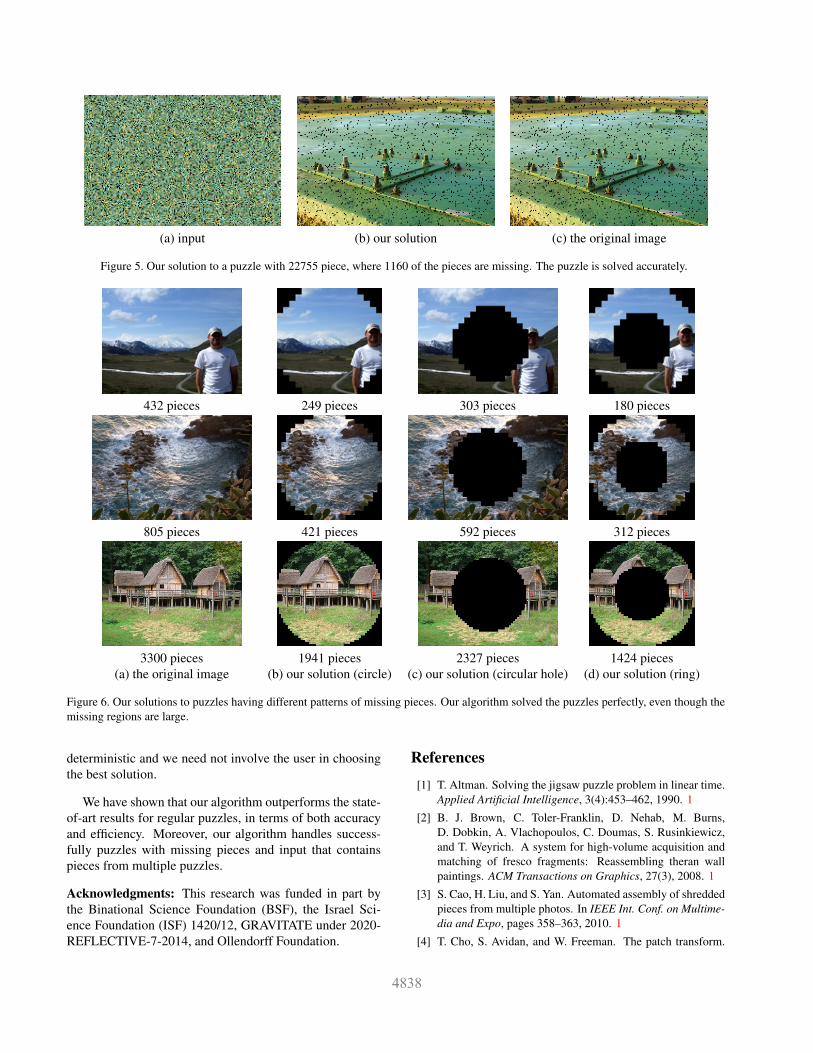
Figure 6 illustrates our results on three different patternsof missing continuous regions, some of which are prettylarge. Patterns with many missing pieces in the center areespecially challenging, because in many cases the salientregion of an image lies in its center.
When the orientation of the pieces is unknown, our algo-rithm achieves a 95.41% success rate with direct compari-
son and 95.4% with neighbors comparison, on the set withpuzzles of 432 pieces . In comparison, the algorithm of [13]achieves a 94.7% and 94.9% success rate respectively.
Finally, Figures 2 and 7 demonstrate the results of ouralgorithm on complex inputs of mixed puzzles with missingpieces, where the size of every puzzle is unknown. Otherexamples can be found in the supplementary material.
Importance of the first piece: To understand the contri-bution of choosing the first piece carefully, we started froma random piece, as done in earlier works, and ran our algo-rithm 10 times on the dataset of Table 1. The average worstresult dropped from 93.8 to 82.09 (direct comparison) &from 95.68 to 94.36 (neighbor comparison).
Limitations: Our algorithm may produce unsatisfactoryresults when the images are smooth or noisy, as demon-strated in Figure 8. It should be mentioned that other al-gorithms fail in these cases as well.
7. Conclusions
In this paper we have introduced a novel algorithm forsquare jigsaw puzzle assembly. We utilized a greedy ap-proach that makes use of a compatibility function betweenpieces. Our function is more accurate and faster to computethan previous functions. Moreover, since greedy solvershighly depend on the initial placement, we take special carewhen choosing the first piece. As a result, our algorithm is
(a) input (b) our solution (c) the original image
Figure 5. Our solution to a puzzle with 22755 piece, where 1160 of the pieces are missing. The puzzle is solved accurately.
432 pieces 249 pieces 303 pieces 180 pieces
805 pieces 421 pieces 592 pieces 312 pieces
3300 pieces 1941 pieces 2327 pieces 1424 pieces(a) the original image (b) our solution (circle) (c) our solution (circular hole) (d) our solution (ring)
Figure 6. Our solutions to puzzles having different patterns of missing pieces. Our algorithm solved the puzzles perfectly, even though themissing regions are large.
deterministic and we need not involve the user in choosingthe best solution.
We have shown that our algorithm outperforms the state-of-art results for regular puzzles, in terms of both accuracyand efficiency. Moreover, our algorithm handles success-fully puzzles with missing pieces and input that containspieces from multiple puzzles.
Acknowledgments: This research was funded in part bythe Binational Science Foundation (BSF), the Israel Sci-ence Foundation (ISF) 1420/12, GRAVITATE under 2020-REFLECTIVE-7-2014, and Ollendorff Foundation.
References
[1] T. Altman. Solving the jigsaw puzzle problem in linear time.Applied Artificial Intelligence, 3(4):453–462, 1990. 1
[2] B. J. Brown, C. Toler-Franklin, D. Nehab, M. Burns,D. Dobkin, A. Vlachopoulos, C. Doumas, S. Rusinkiewicz,and T. Weyrich. A system for high-volume acquisition andmatching of fresco fragments: Reassembling theran wallpaintings. ACM Transactions on Graphics, 27(3), 2008. 1
[3] S. Cao, H. Liu, and S. Yan. Automated assembly of shreddedpieces from multiple photos. In IEEE Int. Conf. on Multime-dia and Expo, pages 358–363, 2010. 1
[4] T. Cho, S. Avidan, and W. Freeman. The patch transform.
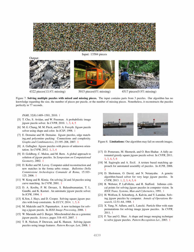
Input: 13584 piecesOutput:
4322 pieces(13.8% missing) 5015 pieces(0% missing) 4517 pieces(9.9% missing)
Figure 7. Solving multiple puzzles with mixed and missing pieces. The input contains parts from 3 puzzles. Our algorithm has noknowledge regarding the size, the number of pieces per puzzle, or the number of missing pieces. Nonetheless, it reconstructs the puzzlesperfectly in 77 seconds.
PAMI, 32(8):1489–1501, 2010. 1[5] T. Cho, S. Avidan, and W. Freeman. A probabilistic image
jigsaw puzzle solver. In CVPR, 2010. 1, 3, 4, 5[6] M. G. Chung, M. M. Fleck, and D. A. Forsyth. Jigsaw puzzle
solver using shape and color. In ICSP, 1998. 1[7] E. Demaine and M. Demaine. Jigsaw puzzles, edge match-
ing,and polyomino packing: Connections and complexity.Graphs and Combinatorics, 23:195–208, 2007. 1
[8] A. Gallagher. Jigsaw puzzles with pieces of unknown orien-tation. In CVPR, 2012. 1, 3, 4
[9] D. Goldberg, C. Malon, and M. Bern. A global approach tosolution of jigsaw puzzles. In Symposium on ComputationalGeometry, 2002. 1
[10] D. Koller and M. Levoy. Computer-aided reconstruction andnew matches in the forma urbis romae. Bullettino DellaCommissione Archeologica Comunale di Roma, 15:103–125, 2006. 1
[11] W. Kong and B. Kimia. On solving 2d and 3d puzzles usingcurve matching. In CVPR, 2001. 1
[12] D. A. Kosiba, P. M. Devaux, S. Balasubramanian, T. L.Gandhi, and K. Kasturi. An automatic jigsaw puzzle solver.In ICPR, 1994. 1
[13] K.Son, J. Hays, and D. Cooper. Solving square jigsaw puz-zles with loop constraints. In ECCV, 2014. 1, 5, 6
[14] M. Makridis and N. Papamarkos. A new technique for solv-ing a jigsaw puzzle. In IEEE Image Processing, 2006. 1
[15] W. Marande and G. Burger. Mitochondrial dna as a genomicjigsaw puzzle. Science, pages 318–415, 2007. 1
[16] T. R. Nielsen, P. Drewsen, and K. Hansen. Solving jigsawpuzzles using image features. Pattern Recogn. Lett, 2008. 1
Figure 8. Limitations: Our algorithm may fail on smooth images.
[17] D. Pomeranz, M. Shemesh, and O. Ben-Shahar. A fully au-tomated greedy square jigsaw puzzle solver. In CVPR, 2011.1, 3, 4, 5, 6
[18] M. Sagiroglu and A. Ercil. A texture based matching ap-proach for automated assembly of puzzles. In ICPR, 2006.1
[19] D. Sholomon, O. David, and N. Netanyahu. A geneticalgorithm-based solver for very large jigsaw puzzles. InCVPR, 2013. 1, 2, 3, 4, 5, 6
[20] R. Webster, P. LaFollette, and R. Stafford. Isthmus criti-cal points for solving jigsaw puzzles in computer vision. InIEEE Trans. Systems, Man and Cybernetics, 1991. 1
[21] H. Wolfson, E. Schonberg, A. Kalvin, and Y. Lamdan. Solv-ing jigsaw puzzles by computer. Annals of Operations Re-search, 12:51–64, 1988. 1
[22] X. Yang, N. Adluru, and L. Latecki. Particle filter with statepermutations for solving image jigsaw puzzles. In CVPR,2011. 1
[23] F. Yao and G. Shao. A shape and image merging techniqueto solve jigsaw puzzles. Pattern Recognition Let., 2003. 1