solutions of dynamic equations on time scales with …
TRANSCRIPT
SOLUTIONS OF DYNAMIC EQUATIONS ON TIME SCALES WITHJUMPS
A thesis submitted to
the Graduate College of
Marshall University
In partial fulfillment of
the requirements for the degree of
Master of Arts in Mathematics
byKayode Daniel Olumoyin
Approved by
Dr. Bonita A. Lawrence, Committee ChairpersonDr. Basant Karna
Dr. Anna Mummert
Marshall UniversityMay 2013
ACKNOWLEDGMENTS
My graduate study at Marshall University has prepared me for my future in Mathematics.
God has helped me through this journey and I praise His name for His faithfulness and
mercies. My parents were my biggest support, to Dad and Mum I say thank you. Dr.
Bonita Lawrence is more than a thesis advisor to me, she is my mentor. I recall that
together with Dr. Alfred Akinsete, she was at Chuck Yeager Airport to receive me when I
first arrived. My work in her differential analyzer lab was the motivation for my thesis on
time scales calculus. Dr. and Dr. (Mrs) Akinsete were my parents in America, 2011 and
2012 Christmas with the Akinsete’s was really awesome.
I enjoyed the classes I took from Dr Anna Mummert and I was excited when she agreed
to be on my thesis committee. I am thankful for her suggestions, which improved the
content and the readabilty of my thesis. I also thank Dr Basant Karna for accepting to
be on my thesis committee, His suggestions were timely and his corrections helped me to
present my work more coherently.
I enjoyed Working with Molly Peterson in the differential analyzer lab. She is so enthu-
siastic about ‘Da Vinci’ which is a similar model to ‘Miles-Diffy’ the differential analyzer
she built while she was an undergraduate. I also thank Dr. Olusola Adeniran. However, I
regret missing my sister’s wedding in August 2012.
ii
CONTENTS
ACKNOWLEDGMENTS ii
ABSTRACT vi
1 Introduction 1
1.1 Historical Development of the Differential Analyzer . . . . . . . . . . . . . . 1
1.2 Construction of the Machine . . . . . . . . . . . . . . . . . . . . . . . . . . 3
1.3 Principle of Integration on ‘Art’ . . . . . . . . . . . . . . . . . . . . . . . . . 5
2 Time Scales Calculus 8
2.1 Basic Definitions . . . . . . . . . . . . . . . . . . . . . . . . . . . . . . . . . 8
2.2 Differentiation . . . . . . . . . . . . . . . . . . . . . . . . . . . . . . . . . . 11
2.3 Integration . . . . . . . . . . . . . . . . . . . . . . . . . . . . . . . . . . . . 13
2.4 First Order Linear Equation . . . . . . . . . . . . . . . . . . . . . . . . . . . 18
2.5 Initial Value Problem . . . . . . . . . . . . . . . . . . . . . . . . . . . . . . 25
3 Solutions of First Order Dynamic Equations on Time Scales with Jumps
on ‘Art’ 32
3.1 Bush Schematic Diagram . . . . . . . . . . . . . . . . . . . . . . . . . . . . 32
3.2 A sequence of Time Scales with Jumps . . . . . . . . . . . . . . . . . . . . . 34
3.3 Plotting the Solution on ‘Art’ . . . . . . . . . . . . . . . . . . . . . . . . . . 35
4 Analytical Solutions of Dynamic Equations on a Time Scale with Jumps 40
4.1 First Order Dynamic Equations with Jumps . . . . . . . . . . . . . . . . . . 40
iii

4.2 Solution of First Order Dynamic Equation using Heaviside Function . . . . 46
4.3 First Order Dynamic Equation with Uniform Jump(s) . . . . . . . . . . . . 49
4.4 First Order Dynamic Equation on an Isolated Time Scale . . . . . . . . . . 51
5 Numerical Solution of a First Order Dynamic Equation with Jumps 54
5.1 Numerical Solutions of a First Order Dynamic Equation on Time Scales with
Non-Uniform Jumps . . . . . . . . . . . . . . . . . . . . . . . . . . . . . . . 55
5.2 Numerical Solution of a First Order Dynamic Equation on a Time Scale with
Uniform Jumps . . . . . . . . . . . . . . . . . . . . . . . . . . . . . . . . . . 59
A Thesis approval from IRB 63
B Python code 65
REFERENCES 75
CURRICULUM VITAE 76
iv

LIST OF FIGURES
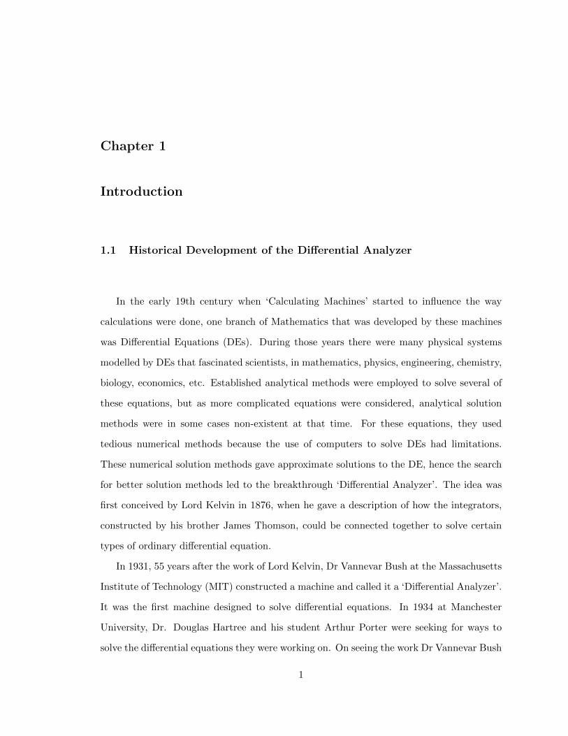
1.1 Dr. Douglas Hartree and Dr. Arthur Porter working on their differential
analyzer. . . . . . . . . . . . . . . . . . . . . . . . . . . . . . . . . . . . . . . 2
1.2 Dr. Bonita Lawrence posing with ‘Art’ at the Grand Opening. . . . . . . . 3
1.3 Principle of integration . . . . . . . . . . . . . . . . . . . . . . . . . . . . . . 4
2.1 Hilger’s Complex Plane . . . . . . . . . . . . . . . . . . . . . . . . . . . . . 19
2.2 Hilger’s Complex Numbers . . . . . . . . . . . . . . . . . . . . . . . . . . . 20
3.1 Bush Schematic Diagram for y∆ptq “ 13yptq . . . . . . . . . . . . . . . . . . 33
3.2 Solution of y∆ “ 13y, y∆p0q “ 1
3 on (a )T0. (b) T1. (c) T2. (d) T3 obtained
on ‘Art’ . . . . . . . . . . . . . . . . . . . . . . . . . . . . . . . . . . . . . . 36
5.1 Solution plot of y∆ptq “ 13yptq, y∆p0q “ 1
3 on (a) T0. (b) T1. (c)T2. (d) T3 58
5.2 Solution of y∆ptq “ 13yptq, y∆p0q “ 1
3 on T0, T1, T2 and T3 . . . . . . . . . 58
5.3 Solution plot of y∆ptq “ 13yptq, y∆p0q “ 1
3 on (a)T10. (b) T11. (c) T12. (d) T13 62
5.4 Solution of y∆ptq “ 13yptq, y∆p0q “ 1
3 on T10, T11, T12 and T13 . . . . . . . . . 62
v
ABSTRACT
SOLUTIONS OF DYNAMIC EQUATIONS ON TIME SCALES WITH JUMPS
Kayode Daniel Olumoyin
To obtain the solution of first order dynamic equations on time scales with jumps, a good
question to ask is, how many initial conditions will be needed? We shall show that you only
need the initial condition that gives you either the initial position or the initial velocity. The
solution at each left scattered point in the time scale can be obtained analytically. With this
approach we shall write the general form of the solution of a first order dynamic equations
on time scales with jumps. To do this we shall use the Hilger derivative, anti-derivatives,
the Hilger Complex plane, the exponential function and the cylinder transformation. We
shall also use the Marshall Differential Analyzer to obtain the solution of the first order
initial value problem as well as calculate the numerical solution to visualize our analytical
solution.
vi
Chapter 1
Introduction
1.1 Historical Development of the Differential Analyzer
In the early 19th century when ‘Calculating Machines’ started to influence the way
calculations were done, one branch of Mathematics that was developed by these machines
was Differential Equations (DEs). During those years there were many physical systems
modelled by DEs that fascinated scientists, in mathematics, physics, engineering, chemistry,
biology, economics, etc. Established analytical methods were employed to solve several of
these equations, but as more complicated equations were considered, analytical solution
methods were in some cases non-existent at that time. For these equations, they used
tedious numerical methods because the use of computers to solve DEs had limitations.
These numerical solution methods gave approximate solutions to the DE, hence the search
for better solution methods led to the breakthrough ‘Differential Analyzer’. The idea was
first conceived by Lord Kelvin in 1876, when he gave a description of how the integrators,
constructed by his brother James Thomson, could be connected together to solve certain
types of ordinary differential equation.
In 1931, 55 years after the work of Lord Kelvin, Dr Vannevar Bush at the Massachusetts
Institute of Technology (MIT) constructed a machine and called it a ‘Differential Analyzer’.
It was the first machine designed to solve differential equations. In 1934 at Manchester
University, Dr. Douglas Hartree and his student Arthur Porter were seeking for ways to
solve the differential equations they were working on. On seeing the work Dr Vannevar Bush
1
Figure 1.1: Dr. Douglas Hartree and Dr. Arthur Porter working on their differentialanalyzer.
was doing, Dr. Hartree and Arthur Porter built a machine similar to Bush’s Figure 1.1.
They used Mecanno components; only for the integrator disc did they use glass. Several
differential analyzers were built afterwards, at University of Cambridge by J.E. Lennard-
Jones in 1935 and at University of Toronto in the early 1950s.
Lord Kelvin used the Planimeter (a machine that shares similarity with the differential
analyzer) built by his brother to predict sea tides. Several years later, Dr. Vannevar
Bush used the ‘differential analyzer’ in his work on differential equations related to electric
power networks. Dr. Douglas Hartree, a physicist and an expert in numerical methods
of computation, used the differential analyzer to solve differential equations occurring in
Atomic Theory. Perhaps the most prominent application of the differential analyzer was
during the Second World War to calculate ‘war related equations’ in USA, UK, Britian
and Germany. For instance, the British used it to calculate the ballistic trajectory of the
German V2 rockets. It however declined in popularity after the war.
Dr. Bonita A. Lawrence, after seeing a model of the differential analyzer in a London
museum with Dr. Clayton Brooks, conceived the idea of building one herself for the purpose
of using it to teach differential equations to her students at Marshall University. Together
2

Figure 1.2: Dr. Bonita Lawrence posing with ‘Art’ at the Grand Opening.
with her team, comprised of Richard Merritt and Saeed Keshavarzian and advice from
Tim Robinson, they started working on building a Differential Analyzer. First they built
a two-integrator machine they called ‘Lizzie’. Following the success of Lizzie, they started
working on a four-integrator differential analyzer in May 2007 and by March 13, 2008,
Marshall University had a working four-integrator machine Figure 1.2. Presently in her
D.A lab, there are three Differential Analyzers. The third is a two - integrator differential
analyzer, a re-design of Lizzie for classroom use, which some of her students named ‘D.A.
Vinci’. Dr. Lawrence has taken ‘Lizzie’ and ‘D.A. Vinci’ to several conferences in the US
and in Europe.
It is to be noted that the differential analyzer can only evaluate differential equations
for which initial conditions are known.
1.2 Construction of the Machine
A differential analyzer consists of several shafts and gears interconnected to solve a particular
differential equation. On a chosen scale, the rotation of each shaft represent the change
of some quantity in the given equation. I will give a description of the four-integrator
differential analyzer at Marshall University. This machine, called ‘Art’ in honour of Dr.
3

Figure 1.3: Principle of integration
Arthur Porter, has four integrator units arranged parallel to one-another, one input/output
table and one output table. On Art, torque amplification of the shaft from the integrating
wheel is achieved with two polarized circular disc arranged in such a way that their rotations
control the amount of light from a light emitting diode (LED). This signal is sent to the
Motorvator (a microprocessor) and determines how much voltage is sent to an electric
motor. Since this is connected to the shaft from the integrator wheel, the torque on this
shaft is amplified and it can then turn the cross shafts. This process of torque amplification
also make use of an H-bridge to allow for bidirectional motion.
A continuously variable gear can act as an integrating mechanism. So, if a shaft B is
driven by a shaft A at a gear ratio n : 1 (that is B makes n turns for one turn of A), and if
the rotation of the driving shaft A is represented by dx, the corresponding rotation of the
driven shaft B is ndx. Since the shafts are arranged so that the gear ratio n is changing
while the driving shaft rotates, the total rotation of B is the sum of the contributions ndx
which isş
n dx [4].
4

1.3 Principle of Integration on ‘Art’
On Art, the integrator unit is comprised of a vertical wheel that can rotate on an horizontal
axis and a horizontal disc which can rotate about a vertical axis through its centre supported
in a movable carriage Figure 1.3. The wheel rests on the disc and the distance of the point
of contact of the wheel on the disc from the centre of the disc can be varied. Suppose the
point of contact of the wheel and disc is a distance y1 from the centre of the disc, measured
in inches. If the disc rotates through a small fraction of a turn dx1, the wheel will rotate
through y1dx1
a , where a is the radius of the wheel, provided there is no slippage in the plane
of the wheel. Now, suppose we fix y1 “ 2a and allow the rod that turns the disc to make
1 turn then the integrator wheel makes 2a˚1a “ 2 turns. When we allow y1 to constantly
vary the total rotation of the integrator wheel is
ż
y1dx1
aturns. (1.3.1)
On each integrator unit there are three shafts:
• The motion of the first shaft causes the disc to rotate. These rotations represent the
changes in the variable of integration.
• The motion of the second shaft turns the displacement lead screw and these rotations
represent the integrand.
• The third shaft is driven by the integrator wheel, through the torque amplifier, and
its rotation represent the integral.
Our interest then is to rewrite the expression for the rotation of the integrator wheel (1.3.1)
in terms of the rotations of the three integrator shafts. To do this let y be the number of
turns of the integrand shaft required to produce a linear displacement y1 of the wheel from
the centre of the disc; y1 changes as the displacement lead screw turns and moves the
5

carriage that holds the disk, so the mathematical relation between y and y1 is given by
y “y1
P, (1.3.2)
where P is the pitch of the displacement screw, the axial distance between the threads.
To achieve a displacement of 1 inch, the displacement of our Whitworth type screw makes
32 turns so that P “ 132 inches{turns. For instance, 1 inch displacement from the position
of the wheel on the disc is acheived by 32 turns of the displacement lead screw.
On Art there is a reduction gear between the shaft representing the variable of integra-
tion and the disc axle. We call this reduction constant K, which is 25 on Art. So if we let
x be the number of turns of the shaft required to produce x1 turns of the disc, then the
mathematical relation between x and x1 is given by
x “x1
K. (1.3.3)
Making substitution for x1 and y1 in (1.3.1) and using (1.3.2) and (1.3.3), we obtain the
rotation of the output shaft from an integrator unit as
KP
a
ż
ydx. (1.3.4)
The term aKP is called the ’integrator constant’.
a
KP“
p1516 inchesq
p25 turnsqp
132 inches{turnsq
“ 75, (1.3.5)
so that the rotations of the output shaft is
1
75
ż
y dx. (1.3.6)
Our goal is to describe the solutions of certain types of dynamic equations on a closed
connected set called a time scale. We will also describe the solutions of these dynamic
equations on a union(s) of connected sets (time scales with jumps). The Marshall Differ-
6

ential Analyzer ‘Art’ will be used to solve these equations on a given connected set and on
a union(s) of connected sets. In the case when our equations are on union(s) of connected
sets, we only need the initial condition that gives us the starting point of our solution.
The starting point after each jump will be given by Art and the use of ‘The Simple Useful
Formula’. First, we start by reviewing basic results about time scales calculus.
7
Chapter 2
Time Scales Calculus
2.1 Basic Definitions
Time scales calculus was initiated in 1988 by Stefan Hilger. It bridges the gap between
continuous and discrete analysis and expands on both theories [2]. Differential equations
are defined on an interval of the set of real numbers while difference equations are defined
on discrete sets. However, some physical systems are modelled by what is called dynamic
equations because they are either differential equations, difference equations or a combi-
nation of both. This means that dynamic equations are defined on connected, discrete or
combination of both types of sets. Hence, time scales calculus provides a generalization of
differential and difference analysis. The following introductory material can be found in [2]
where complete proofs are provided.
Definition 1. A time scale is an arbitrary non - empty closed subset of the real numbers.
Example 1. Examples of time scales include:
• The real numbers R
• The integers Z
• The natural numbers N
• The non - negative integers N0
8

Other examples of time scales are
• r0, 1s
• r0, 1s Y r2, 3s
• the Cantor set.
Non examples of time scales include the set of rational numbers Q, complex numbers
C, and the open interval from 0 to 1 p0, 1q. We denote a general time scales as T. We
are concerned with classifying points in a time scales. To do this, we need operators that
moves us forward or backward, enabling us to jump over the gaps (if there are any) in our
time scale T. Specifically, we are often concerned with moving to the next point or previous
point in the time scale T. Hence we have the definition below.
Definition 2. Let T be a time scale. For t P T, we define the forward jump operator
σ : TÑ T by
σptq :“ infts P T : s ą tu,
while the backward jump operator ρ : TÑ T by
ρptq :“ supts P T : s ă tu.
The forward jump operator gives you the ‘next’ point in your time scale. In some cases,
σptq “ t; this occurs when t is in an interval or when t = sup T. On the other hand, the
backward jump operator gives you the ‘previous’ point in your time scale. In some cases,
ρptq “ t; this happens when t is in an interval or when t = inf T.
We use jump operators to classify points in the time scale. The points are either dense
in the set or have measurable gaps (jumps) between them. If a point t has a jump after
it, that is σptq ą t, we define the point t as right-scattered. Similarly, if that point t has
a jump before it, that is ρptq ă t, we define the point t as left-scattered. Points that are
both left and right scattered are called isolated. In contrast, if there is no discernable jump
between a point t and the next point to t in T, then σptq “ t, and we call t right-dense.
9
Likewise, if there is no discernable jump between a point t and the previous point to t in
T then ρptq “ t, and we call t left-dense. Points that are right-dense and left-dense at the
same time are called dense.
For a discrete set of points, we define the change in position between consecutive points
as µptq :“ σptq ´ t and we call µptq the graininess function. Note that the value of µptq
will always be in the interval r0,8q. The graininess function in a connected interval is also
defined as µptq :“ σptq ´ t but always equal 0.
In order to proceed to the concept of differentiation and integration on a time scale, we
shall define the set Tk, derived from the time scale T as follows: If T has a left-scattered
maximum m, then Tk “ T´ tmu. Else, Tk “ T. In general,
Tk :“
$
’
’
&
’
’
%
TzpρpsupTq, supTs supT ă 8
T supT “ 8.
Lastly, if f : TÑ R is a function, then we define the function fσ : TÑ R by
fσptq “ fpσptqq @ t P T.
Example 2. If we consider the time scales T “ R and T “ Z and classify their points using
the jump operators, we have the following.
(i) If T “ R, then we have for any t P R
σptq “ infts P R : s ą tu “ infpt,8q “ t
Similarly ρptq “ t. Hence every point t P R is dense. The graininess function µ turns out
to be
µptq “ σptq ´ t “ t´ t “ 0 for all t P T.
(ii) If T “ Z, then we have for any t P Z
σptq “ infts P Z : s ą tu “ infpt` 1, t` 2, t` 3, . . . q “ t` 1
10
and similarly ρptq “ t´ 1. Hence every point t P Z is isolated. The graininess function µ in
this case is
µptq “ σptq ´ t “ t` 1´ t “ 1 for all t P T.
2.2 Differentiation
For f : TÑ R be a function, we define the delta or Hilger derivative of f at a point t P Tk
as follows:
Definition 3. (Bohner and Peterson [2]) Assume f : T Ñ R is a function and let t P Tk.
Then we define f∆ptq to be the number (provided it exists) with the property that given any
ε ą 0, there is a neighborhood U of t (i.e., U “ pt´ δ, t` δq XT for some δ ą 0) such that
|rfpσptqq ´ fpsqs ´ f∆ptqrσptq ´ ss| ď ε|σptq ´ s| for all s P U
We call f∆ptq the delta or Hilger derivative of f at t.
The following theorem provides some useful characterizations of delta differentiable func-
tions.
Theorem 3. (Bohner and Peterson [2]) Assume f : TÑ R be a function and t P Tk. Then
we have the following:
1. If f is differentiable at t, then f is continuous at t.
2. If f is continuous at t and t is right-scattered, then f is differentiable at t with
f∆ptq “fpσptqq ´ fptq
µptq.
3. If t is right-dense, then f is differentiable at t if and only if the limit
limsÑt
fptq ´ fpsq
t´ s
11

exists as a finite number. In this case
f∆ptq “ limsÑt
fptq ´ fpsq
t´ s.
4. If f is differentiable at t, then
fpσptqq “ fptq ` µptqf∆ptq.
Which is usually called the ‘Simple Useful Formula’.
The following theorem establishes the linearity of the delta derivative, as well as the
product and quotient rules for delta differentiation.
Theorem 4. (Bohner and Peterson [2]) Assume f, g : T Ñ R is differentiable at t P Tk.
Then:
1. The sum f ` g : TÑ R is differentiable at t with
pf ` gq∆ptq “ f∆ptq ` g∆ptq.
2. For any constant α, αf : TÑ R is differentiable at t with
pαfq∆ptq “ αf∆ptq.
3. The product fg : TÑ R is differentiable at t with
pfgq∆ptq “ f∆ptqgptq ` fpσptqqg∆ptq “ fptqg∆ptq ` f∆ptqgpσptqq.
4. If fptqfpσptqq ‰ 0, then 1f is differentiable at t with
ˆ
1
f
˙∆
ptq “ ´f∆ptq
fptqfpσptqq.
12

5. If gptqgpσptqq ‰ 0, then fg is differentiable at t and
ˆ
f
g
˙∆
ptq “f∆ptqgptq ´ fptqg∆ptq
gptqgpσptqq.
If we consider functions of the form, fptq “ pt ´ αqm, and gptq “ 1pt´αqm for example,
we define their delta derivatives as follows.
Theorem 5. (Bohner and Peterson [2]) Let α be constant and m P N.
1. For f defined by fptq “ pt´ αqm we have
f∆ptq “m´1ÿ
v“0
pσptq ´ αqvpt´ αqm´1´v.
2. For g defined by gptq “ 1pt´αqm we have
g∆ptq “ ´m´1ÿ
v“0
1
pσptq ´ αqm´vpt´ αqv`1,
provided pt´ αqpσptq ´ αq ‰ 0.
Having described what it means for a function to be differentiable at a point t in T, we
are ready to describe the concept of integration.
2.3 Integration
In this section, we will describe classes of functions that are ‘integrable’. We begin with the
following definitions.
Definition 4. (Bohner and Peterson [2]) A function f : TÑ R is called regulated provided
its right-sided limits exist (finite) at all right-dense points in T and its left-sided limits exist
(finite) at all left-dense points in T.
Definition 5. (Bohner and Peterson [2]) A function f : T Ñ R is called rd-continuous
provided it is continuous at each right-dense point in T and its left-sided limits exist (finite)
13

at all left-dense points in T. The set of rd-continuous functions f : TÑ R is denoted by
Crd “ CrdpTq “ CrdpT,Rq.
Now we have the following theorem that describes the relationship between continuous,
rd-continuous and regulated functions, f , defined on a time scale, T.
Theorem 6. (Bohner and Peterson [2]) Assume f : TÑ R.
1. If f is continuous, then f is rd-continuous.
2. If f is rd-continuous, then f is regulated.
3. The jump operator σ is rd-continuous.
4. If f is regulated or rd-continuous, then so is fσ.
5. Assume f is continuous. If g : T Ñ R is regulated or rd-continuous, then f ˝ g has
that property too.
Next we will define pre-differentiable functions with regions of differentiation D.
Definition 6. (Bohner and Peterson [2]) A continuous function f : T Ñ R is called pre-
differentiable with (region of differentiation) D, provided D Ă Tκ, TκzD is countable and
contains no right-scattered elements of T, and f is differentiable at each t P D.
Now if we have a pre-differentiable function, the next theorem states that it is the
pre-antiderivatives of some regulated function f .
Theorem 7. (Bohner and Peterson [2]) Let f be regulated. Then there exists a function F
which is pre-differentiable with region of differentiation D such that
F∆ptq “ fptq holds for all t P D.
Utilizing the pre-antiderivative of a regulated function f we define the anti-dervative of
f .
14
Definition 7. (Bohner and Peterson [2]) Assume f : TÑ R is a regulated function. Any
function F as in Theorem 7 is called a pre-antiderivative of f . We define the indefinite
integral of a regulated function f by
ż
fptq∆t “ F ptq ` C,
where C is an arbitrary constant and F is a pre-antiderivative of f . We define the Cauchy
integral byż s
rfptq∆t “ F psq ´ F prq for all r, s P T.
A function F : TÑ R is called an antiderivative of f : TÑ R provided
F∆ptq “ fptq holds for all t P Tk.
Next we have a theorem that offers a condition that insures the existence of an an-
tiderivative for a function f .
Theorem 8. (Bohner and Peterson [2]) Every rd-continuous function has an antiderivative.
In partcular if t0 P T, then F defined by
F ptq ”
ż t
t0
fpτq∆τ for t P T
is an antiderivative of f.
Theorem 9. (Bohner and Peterson [2]) if f P Crd and t P Tκ, then
ż σptq
tfpτq4τ “ µptqfptq.
The following theorem offers us properties of the antiderivative.
Theorem 10. (Bohner and Peterson [2]) If a, b, c P T, α P R, and f, g P Crd, then
1.şba rfptq ` gptqs4t “
şba fptq4t`
şba gptq4t;
2.şba pαfptqq4t “ α
şba fptq4t;
15

3.şba fptq4t “ ´
şab fptq4t;
4.şba fptq4t “
şca fptq4t`
şbc fptq4t;
5.şba fpσptqqg
∆ptq4t “ pfgqpbq ´ pfgqpaq ´şba f
∆ptqgptq4t;
6.şba fptqg
∆ptq4t “ pfgqpbq ´ pfgqpaq ´şba f
∆ptqgpσptqq4t;
7.şaa fptq4t “ 0;
8. If | fptq |ď gptq on ra, bq, then |şba fptq4t |ď
şba gptq4t;
9. If fptq ě 0 for all a ď t ă b, thenşba fptq4t ě 0
The following theorem that gives us the antiderivative on some particular time scales.
Theorem 11. (Bohner and Peterson [2]) Let a, b P T and f P Crd
1. If T “ R, thenż b
afptq4t “
ż b
afptqdt,
where the integral on the right is the usual Riemann integral from calculus.
2. If ra, bs :“ tt P T : a ď t ď bu consists of only isolated points, then
ż b
afptq4t “
$
’
’
’
’
’
’
&
’
’
’
’
’
’
%
ř
tPra,bq µptqfptq if a ă b
0 if a “ b
´ř
tPrb,aq µptqfptq if a ą b
3. If T “ hZ = thk : k P Zu, where h ą 0, then
ż b
afptq4t “
$
’
’
’
’
’
’
&
’
’
’
’
’
’
%
ř
bh´1
k“ ahfpkhqh if a ă b
0 if a “ b
´ř
bh
k“ ah´1 fpkhqh if a ą b
16

4. If T “ Z, then
ż b
afptq4t “
$
’
’
’
’
’
’
&
’
’
’
’
’
’
%
řb´1t“a fptq if a ă b
0 if a “ b
´řa´1t“b fptq if a ą b
The improper integral is defined as follows:
Definition 8. (Bohner and Peterson [2]) If a P T, supT “ 8, and f is rd-continuous on
ra,8q, then we define the improper integral by
ż 8
afptq4t “ lim
bÑ8
ż b
afptq4t
provided this limit exists, and we say that the improper integral converges in this case. If
this limit does not exist, then we say that the improper integral diverges.
The chain rule has two forms in time scales calculus. Both are stated in the following
theorems. The second is due to Christian P :otzsche, who derived it in 1998.
Theorem 12. (Bohner and Peterson [2]) Assume g : R Ñ R is continuous, g : T Ñ R is
delta differentiable on Tκ, and f : R Ñ R is continuously differentiable. Then there exists
c in the real interval rt, σptqs with
pf ˝ gq∆ptq “ f 1pgpcqqg∆ptq. (2.3.1)
Where f 1 is the usual derivative of f .
Theorem 13. (Bohner and Peterson [2]) Let f : RÑ R be continuously differentiable and
suppose g : TÑ R is delta differentiable. Then f ˝ g : TÑ R is delta differentiable and the
formula
pf ˝ gq∆ptq “
"ż 1
0f 1`
gptq ` hµptqg∆ptq˘
dh
*
g∆ptq
holds.
17
2.4 First Order Linear Equation
We intend to describe the solutions of first order dynamic equations on some selected time
scales. However, to do this we need to have a general form for a first order dynamic equation.
We offer this in the next definition.
Definition 9. (Bohner and Peterson [2]) Suppose f : Tˆ R2 Ñ R. Then the equation
y∆ “ fpt, y, yσq (2.4.1)
is called a first order dynamic equation, sometimes also a differential equation. If
fpt, y, yσq “ f1ptqy ` f2ptq or fpt, y, yσq “ f1ptqy
σ ` f2ptq
for functions f1 and f2, then (2.4.1) is called a linear equation. A function y : T Ñ R is
called a solution of 2.4.1 on Tκ if
y∆ptq “ fpt, yptq, ypσptqqq is satisfied for all t P Tκ.
The general solution of (2.4.1) is defined to be the set of all solutions of (2.4.1). Given
t0 P T and y0 P R, the problem
y∆ “ fpt, y, yσq, ypt0q “ y0
is called an initial value problem (IVP) and a solution y of (2.4.1) with ypt0q “ y0 is called
a solution of this IVP.
In the next section, we will describe the solution of the first order dynamic equation
y∆ “ pptqyptq with ypt0q “ y0.
We shall call this solution the exponential function. First, we will define the components of
the Hilger Complex Plane.
18
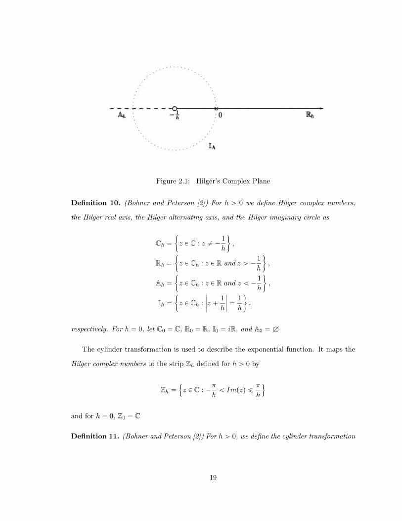
Figure 2.1: Hilger’s Complex Plane
Definition 10. (Bohner and Peterson [2]) For h ą 0 we define Hilger complex numbers,
the Hilger real axis, the Hilger alternating axis, and the Hilger imaginary circle as
Ch “"
z P C : z ‰ ´1
h
*
,
Rh “"
z P Ch : z P R and z ą ´1
h
*
,
Ah “"
z P Ch : z P R and z ă ´1
h
*
,
Ih “"
z P Ch :
ˇ
ˇ
ˇ
ˇ
z `1
h
ˇ
ˇ
ˇ
ˇ
“1
h
*
,
respectively. For h “ 0, let C0 “ C, R0 “ R, I0 “ iR, and A0 “ H
The cylinder transformation is used to describe the exponential function. It maps the
Hilger complex numbers to the strip Zh defined for h ą 0 by
Zh “!
z P C : ´π
hă Impzq ď
π
h
)
and for h “ 0, Z0 “ C
Definition 11. (Bohner and Peterson [2]) For h ą 0, we define the cylinder transformation
19

Figure 2.2: Hilger’s Complex Numbers
ξh : Ch ÝÑ Zh by
ξhpzq “1
hLogp1` zhq, (2.4.2)
where Log is the principal logarithm function. We also define the inverse transformation by
ξ´1h pzq “
1
hpezh ´ 1q (2.4.3)
and for h “ 0, we define ξ0pzq “ z for all z in C .
We shall define the generalized exponential function for functions classified as regressive.
Next, we present what it means for a function to be regressive.
Definition 12. (Bohner and Peterson [2]) We say that a function p : T ÝÑ R is regressive
provided
1` µptqpptq ‰ 0 for all t P Tκ (2.4.4)
holds. The set of all regressive and rd-continuous function f : T ÝÑ R will be denoted by
20
R “ RpTq “ RpT,Rq.
Definition 13. (Bohner and Peterson [2]) If p P R, then we define the exponential function
by
eppt, sq “ exp
ˆż t
sξµpτqpppτqq∆τ
˙
for s, t P T (2.4.5)
Lemma 14. (Bohner and Peterson [2]) If p P R, then the semigroup property
eppt, rqeppr, sq “ eppt, sq for all r, s, t P T (2.4.6)
is satisfied.
Definition 14. (Bohner and Peterson [2]) If p P R, then the first order linear dynamic
equation
y∆ “ pptqy (2.4.7)
is called regressive.
We are now ready for the theorem that describes the solution of the first order linear
dynamic equation p2.4.7q on a time scale T. The proof, found in [2], is presented with more
details to offer the reader a general structure of a proof on a time scale T.
Theorem 15. (Bohner and Peterson [2]) Suppose y4 “ pptqy is regressive and fix t0 in T.
Then epp., t0q is a solution of the initial value problem
y4 “ pptqy, ypt0q “ 1 on T. (2.4.8)
Proof. Fix t0 and assume y∆ “ pptqy is regressive. First note that
eppt0, t0q “ 1. (2.4.9)
It remains to show that eppt, t0q satisfies the dynamic equation y4 “ pptqy. Fix t P Tκ.
There are two cases:
Case 1. Assume σptq ą t, (t is right scattered).
21

For s = t0, eppt, sq is defined as eppt, t0q = exp´
ştt0ξµpτqpppτqq∆τ
¯
for t0, t P T. Now using
Lemma 14 and the inverse transformation (2.4.3), we obtain
e4p pt, t0q “exp
´
şσptqt0
ξµpτqpppτqq∆τ¯
´ exp´
ştt0ξµpτqpppτqq∆τ
¯
µptq
“exp
´
ştt0ξµpτqpppτqq∆τ `
şσptqt ξµpτqpppτqq∆τ
¯
´ exp´
ştt0ξµpτqpppτqq∆τ
¯
µptq
“
exp´
ştt0ξµpτqpppτqq∆τ
¯
exp´
şσptqt ξµpτqpppτqq∆τ
¯
´ exp´
ştt0ξµpτqpppτqq∆τ
¯
µptq
“
´
exp´
şσptqt ξµpτqppτq∆τ
¯
´ 1¯
µptqeppt, t0q
“
`
expppσptq ´ tqξµptqppptqqq ´ 1˘
µptqeppt, t0q
“
`
exppµptqξµptqppptqqq ´ 1˘
µptqeppt, t0q
“ ξ´1µptqpξµptqppptqqq ¨ eppt, t0q
“ pptq ¨ eppt, t0q.
Case 2. Next we assume σptq “ t (t is right dense). If yptq “ eppt, t0q, we want to show that
y4ptq “ pptqyptq.
22

From Lemma 14 and for s P T we have that
| yptq ´ ypsq ´ pptqyptqpt´ sq | “ |eppt, t0q ´ epps, t0q ´ pptqeppt, t0qpt´ sq|
“| eppt, t0q | ¨ |1´ epps, tq ´ pptqpt´ sq|
“| eppt, t0q | ¨ | 1´
ż t
sξµpτqpppτqq∆τ ´ epps, tq
`
ż t
sξµpτqpppτqq∆τ ´ pptqpt´ sq |
ď| eppt, t0q | ¨
ˇ
ˇ
ˇ
ˇ
1´
ż t
sξµpτqpppτqq∆τ ´ epps, tq
ˇ
ˇ
ˇ
ˇ
` | eppt, t0q | ¨
ˇ
ˇ
ˇ
ˇ
ż t
sξµpτqpppτqq∆τ ´ pptqpt´ sq
ˇ
ˇ
ˇ
ˇ
ď| eppt, t0q | ¨
ˇ
ˇ
ˇ
ˇ
1´
ż t
sξµpτqpppτqq∆τ ´ epps, tq
ˇ
ˇ
ˇ
ˇ
` | eppt, t0q | ¨
ˇ
ˇ
ˇ
ˇ
ż t
s
“
ξµpτqpppτqq ´ ξ0ppptqq‰
∆τ
ˇ
ˇ
ˇ
ˇ
.
Let ε ą 0 be given. We now show that there is a neighborhood U of t so that for s P U
the right hand side of the last inequality is less than ε | t´s | and the proof will be complete.
Since σptq “ t and p P Crd, it follows that
limτÑt
ξµpτqpppτqq “ ξ0ppptqq. (2.4.10)
This implies that there is a neighborhood U1 of t such that
ˇ
ˇξµpτqpppτqq ´ ξ0ppptqqˇ
ˇ ăε
3 | eppt, t0q |for all τ P U1.
Let s P U1. Then
| eppt, t0q | .
ˇ
ˇ
ˇ
ˇ
ż t
srξµpτqpppτqq ´ ξ0ppptqqs∆τ
ˇ
ˇ
ˇ
ˇ
ďε
3|t´ s| . (2.4.11)
23
Next, by L’Hopital’s rule,
limzÑ0
1´ z ´ e´z
z“ 0.
So there is a neighborhood U2 of t so that if s P U2, then
ˇ
ˇ
ˇ
ˇ
ˇ
1´şts ξµpτq ´ epps, tq
şts ξµpτqpppτqq∆τ
ˇ
ˇ
ˇ
ˇ
ˇ
ă ε‹, (2.4.12)
where
ε‹ “ min
"
1,ε
1` 3 | pptqeppt, t0q |
*
.
Let s P U “ U1 X U2. Then
| eppt, t0q | ¨
ˇ
ˇ
ˇ
ˇ
1´
ż t
sξµpτqpppτqq∆τ ´ epps, tq
ˇ
ˇ
ˇ
ˇ
ă| eppt, t0q | ¨ε‹
ˇ
ˇ
ˇ
ˇ
ż t
sξµpτqpppτqq∆τ
ˇ
ˇ
ˇ
ˇ
ď| eppt, t0q | ¨ε‹
"ˇ
ˇ
ˇ
ˇ
ż t
srξµpτqpppτqq ´ ξ0ppptqqs∆τ
ˇ
ˇ
ˇ
ˇ
` | pptq | |t´ s|
*
ď| eppt, t0q | ¨
ˇ
ˇ
ˇ
ˇ
ż t
srξµpτqpppτqq ´ ξ0ppptqqs∆τ
ˇ
ˇ
ˇ
ˇ
` | eppt, t0q | ε‹ | pptq || t´ s |
ďε
3| t´ s | ` | eppt, t0q | ε
‹ | pptq || t´ s |
ďε
3| t´ s | `
ε
3|t´ s|
“2ε
3| t´ s |
so that
| yptq ´ ypsq ´ pptqyptqpt´ sq | “2ε
3| t´ s | `
ε
3| t´ s |
“ ε | t´ s | .
And so if yptq “ eppt, t0q then y∆ptq “ pptqyptq, where ypt0q “ 1 on T.
The above theorem confirms the existence of a solution. We will show that this solution
is the only solution of the initial value problem (2.4.8)
Theorem 16. (Bohner and Peterson [2]) If ( 2.4.7) is regressive, then the only solution of
(2.4.8) is given by epp¨, toq.
24

Proof. Assume y is a solution of (2.4.8) and consider the quotient yepp¨,t0q
.
By Theorem 4(5) we have
ˆ
y
epp., t0q
˙4ptq “
yptq4eppt, t0q ´ yptqe4p pt, t0q
eppt, t0qeppσptq, t0q
“pptqyptqeppt, t0q ´ yptqpptqeppt, t0q
eppt, t0qeppσptq, t0q
“ 0
We know that if f is a pre-differentiable function and f∆ptq “ 0 then f is a constant
function. So yptqeppt,t0q
is a constant function. Hence yptqeppt,t0q
”ypt0q
eppt0,t0q“ 1
1 and therefore
y “ epp¨, t0q.
2.5 Initial Value Problem
Consider the homogeneous equation,
y∆ “ pptqyptq (2.5.1)
on a time scale T. Our previous discussion gives us the following theorem.
Theorem 17. (Bohner and Peterson [2]) Suppose (2.5.1) is regressive. Let t0 P T and
y0 P R. The unique solution of the initial value problem
y∆ “ pptqyptq, ypt0q “ y0, (2.5.2)
is given by
yptq “ eppt, t0qy0.
If we consider time scales, R, Z, hZ and qN0 and we solve initial value problem (2.5.2)
for these time scales using the exponential function we obtain the following solutions [1]:
Example 18. Let T “ R, then µptq “ 0. If (2.5.1) is regressive, then the solution of the
25
IVP y∆ “ pptqyptq, where ypt0q “ 1 by Theorem 17 is
yptq “ eppt, t0q “ eştt0ξ0pppτqqp∆τq
“ eştt0ppτq∆τ
,
and
ypt0q “ eppt0, t0q “ eşt0t0ppτqp∆τq
“ 1.
Now if pptq “ a (a constant)
yptq “ eapt, t0q “ eştt0ap∆τq
“ eapt´t0q
and, if t0 “ 0,
yptq “ eapt, 0q “ eşt0 ap∆τq
“ eat.
Thus, if a “ 1,
yptq “ eapt, 0q “ et.
The above result for T “ R is consistent with solving the IVP y1 “ pptqy where yp0q “ 1
and pptq ” a.
Example 19. If T “ Z, then µptq “ 1. And Suppose (2.5.1) is regressive, then the solution
of the IVP ∆yptq “ pptqyptq, where ypt0q “ 1 and ∆yptq “ ypt ` 1q ´ yptq r5s by Theorem
17 and Theorem 11(4) is
yptq “ eppt, t0q “ eřt´1τ“t0
ξ1pppτqq.
If t0 ă t,t´1ÿ
τ“t0
ξ1pppτqq “t´1ÿ
τ“t0
Logp1` ppτqq,
26
by the definition of cylinder transformation, and
t´1ÿ
τ“t0
Logp1` ppτqq “ Logt´1ź
τ“t0
p1` ppτqq.
So,
eppt, t0q “ eLog
śt´1τ“t0
p1`ppτqq
“
t´1ź
τ“t0
p1` ppτqq.
If t0 “ t then
eppt, t0q “ eppt, tq “ e0 “ 1.
If t0 ą t then
eppt, t0q “1
eppt0, tq
“1
eřt0´1τ“t ξ1pppτqq
“1
eřt0´1τ“t Logp1`ppτqq
“1
eLogśt0´1τ“t p1`ppτqq
“1
śt0´1τ“t p1` ppτqq
.
Hence,
eppt, t0q “
$
’
’
’
’
’
’
&
’
’
’
’
’
’
%
śt´1τ“t0
p1` ppτqq when t0 ă t
1 when t0 “ t
1śt0´1τ“t p1`ppτqq
when t0 ą t.
Now if pptq “ a (a constant) and a ‰ ´1
eapt, t0q “ p1` aqt´t0 .
27
If t0 “ 0, then
eapt, 0q “ p1` aqt.
If a “ 1, then
e1pt, 0q “ 2t.
The above result for T “ Z is consistent with solving the difference equation ∆yptq “
ypt` 1q ´ yptq “ pptqypt` 1q.
Example 20. If T “ hZ, where hZ “ thk|k P Zu for some h ą 0 then µptq “ h. And
Suppose (2.5.1) is regressive, then the solution of the IVP ypt`hq´yptqh “ pptqyptq, where
ypt0q “ 1 by Theorem 17 is
yptq “ eppt, t0q “ eřt´1τ“t0
ξhpppτqq.
If t0 ă t,t´1ÿ
τ“t0
ξhpppτqq “t´1ÿ
τ“t0
1
hLogp1` ppτqhq,
by the definition of cylinder transformation, and
t´1ÿ
τ“t0
1
hLogp1` ppτqhq “
1
h
t´1ÿ
τ“t0
Logp1` ppτqhq
“1
hLog
t´1ź
τ“t0
p1` ppτqhq
“ Log
«
t´1ź
τ“t0
p1` ppτqhq
ff1h
.
So,
eppt, t0q “ eLog
”
śt´1τ“t0
p1`ppτqhqı 1h
“
«
t´1ź
τ“t0
p1` ppτqhq
ff1h
.
28

If t0 “ t, then
eppt, t0q “ eppt, tq “ e0 “ 1.
If s ą t, then
eppt, t0q “1
eppt0, tq
“1
eřt0´1τ“t ξhpppτqq
“1
eřt0´1τ“t
1hLogp1`ppτqhq
“1
eLog
”
śt0´1τ“t p1`ppτqhq
ı 1h
“1
”
śt0´1τ“t p1` ppτqhq
ı1h
.
Hence,
eppt, t0q “
$
’
’
’
’
’
’
’
&
’
’
’
’
’
’
’
%
”
śt´1τ“t0
p1` ppτqhqı
1h
when t0 ă t
1 when t0 “ t
1”
śt0´1τ“t p1`ppτqhq
ı 1h
when t0 ą t.
Now, if pptq “ a (a constant) and h “ 1n for some natural number n P N and a ‰ ´1
eapt, t0q “´
1`a
n
¯npt´t0q.
If t0 “ 0, then
eapt, 0q “´
1`a
n
¯nt.
as nÑ8´
1`a
n
¯nÑ e
and so
eapt, 0q Ñ et.
29
Example 21. If T “ qN0 , where q ą 1 and qN0 “ tqk|k P Nu Y t0u then µptq “ pq ´ 1qt.
And Suppose (2.5.1) is regressive, then the solution of the IVP ypqtq´yptqpq´1qt “ pptqyptq, where
yp1q “ 1 by Theorem 17 is
yptq “ eppqk, 1q “
k´1ź
ν“0
r1` pq ´ 1qqνppqνqs .
If we define p : TÑ R,
pptq “1´ t
pq ´ 1qt2for t P T,
then
eppqk, 1q “
k´1ź
ν“0
„
1` pq ´ 1qqν1´ qν
pq ´ 1qq2ν
“
k´1ź
ν“0
„
1`1´ qν
pq ´ 1qqν
“
k´1ź
ν“0
1
qν
“1
qkpk´1q{2
“ q´k2
2 ¨ qk2
“a
qk exp
"
´k2
2ln q
*
“a
qk exp
"
´pk ln qq2
2 ln q
*
so that
eppt, 1q “?t exp
"
´pln tq2
2 ln q
*
.
30

To verify,
y∆ “ypqtq ´ yptq
pq ´ 1qt
“
?qt exp
!
´pln qtq2
2 ln q
)
´?t exp
!
´pln tq2
2 ln q
)
pq ´ 1qt
“q
12
?t exp
!
´pln tq2`2 ln t ln q`pln qq2
2 ln q
)
´?t exp
!
´pln tq2
2 ln q
)
pq ´ 1qt
“q
12
?t exp
!
´pln tq2
2 ln q
)
¨ t´1 ¨ q´12 ´
?t exp
!
´pln tq2
2 ln q
)
pq ´ 1qt
“q
12 ¨ t´1 ¨ q´
12 ´ 1
pq ´ 1qt
?t exp
"
´pln tq2
2 ln q
*
“t´1 ´ 1
pq ´ 1qt¨t
t
?t exp
"
´pln tq2
2 ln q
*
“1´ t
pq ´ 1qt2¨?t exp
"
´pln tq2
2 ln q
*
“ pptq ¨ yptq.
31

Chapter 3
Solutions of First Order Dynamic Equations on Time Scales
with Jumps on ‘Art’
The solution of the initial value problem (2.5.2) on a time scale T with jumps was first solved
using the Marshall Differential Analyzer ‘Art’ before describing the analytical solution.
However, we did remark in the introduction that the differential analyzer can only solve
differential equations with known initial conditions. Hence, our task is to solve the modified
dynamic equation
y∆ptq “1
3yptq, y∆p0q “
1
3(3.0.1)
on T “ r0, 1s.
3.1 Bush Schematic Diagram
Dr Vannevar Bush developed a way to represent the connections between integrators on
a differential analyzer, which he called the ‘Bush Schematic Diagram’. In the Bush’s
schematic, the rectangular boxes represent the integrators, the circles represents the disc
while the line across the circles represent the wheel. The shaded region attached to each
circle, as seen in the Bush’s schematics, represents the carriage on which the disc sits and
the horizontal lines represents the connecting rods. We labeled the first rod the independent
variable and we scaled it to (250t). This means it takes the independent variable rod 250
rotations for a unit of our independent variable t. The motion of this rod rotates the disc.
The second rod, we labeled y∆, which is the integrand; this we scaled as (75y∆). The
32

Figure 3.1: Bush Schematic Diagram for y∆ptq “ 13yptq
motion on this rod turns the lead screw and it drives the carriage. The motion on the third
rod is as a result of the motion transfered from the disc by friction to the wheel which is
then amplified by our system of torque amplification.
In the Introduction, I discussed how we obtained the ‘integrator constant’ (1.3.5). On
‘Art’ it takes the independent variable rod 75 rotations for a unit of our independent variable.
The counters on each integrator gears the motion up by 103 . Therefore 75 rotations of the
independent variable rod is equivalent to 250 rotations of the counter. Hence, the rotations
of the output rod, the third rod as seen in our Bush’s schematic is
1
250
ż
75y∆ dp250tq “ 75yptq.
The 3 to 1 gearing in our Bush Schematic represents the gearing down of the motion of
75yptq by a fraction of 13 and so we obtain 25yptq. We complete this connection to the
output rod 25yptq by joining the integrand rod 75y∆, or 75y∆ “ 25y.
33
3.2 A sequence of Time Scales with Jumps
To solve (3.0.1) on ‘Art’, we first chose our time scale T “ r0, 1s. The jumps in the time
scale are created using the sequence below [6];
Ti “iď
k“0
„ˆ
1
2i` 1
˙
p2kq,
ˆ
1
2i` 1
˙
p2k ` 1q
where i “ 1, 2, 3, . . . is the number of jumps.
When there is no jump, we have
T0 “
0ď
k“0
„ˆ
1
p2ˆ 0q ` 1
˙
p2kq,
ˆ
1
p2ˆ 0q ` 1
˙
p2k ` 1q
“
„ˆ
1
p2ˆ 0q ` 1
˙
p2ˆ 0q,
ˆ
1
p2ˆ 0q ` 1
˙
pp2ˆ 0q ` 1q
“ r0, 1s;
one jump
T1 “
1ď
k“0
„ˆ
1
p2ˆ 1q ` 1
˙
p2kq,
ˆ
1
p2ˆ 1q ` 1
˙
p2k ` 1q
“
„ˆ
1
p2ˆ 1q ` 1
˙
p2ˆ 0q,
ˆ
1
p2ˆ 1q ` 1
˙
pp2ˆ 0q ` 1q
Y
„ˆ
1
p2ˆ 1q ` 1
˙
p2ˆ 1q,
ˆ
1
p2ˆ 1q ` 1
˙
pp2ˆ 1q ` 1q
“
„
0,1
3
Y
„
2
3, 1
;
34
two jumps
T2 “
2ď
k“0
„ˆ
1
p2ˆ 2q ` 1
˙
p2kq,
ˆ
1
p2ˆ 2q ` 1
˙
p2k ` 1q
“
„ˆ
1
p2ˆ 2q ` 1
˙
p2ˆ 0q,
ˆ
1
p2ˆ 2q ` 1
˙
pp2ˆ 0q ` 1q
Y
„ˆ
1
p2ˆ 2q ` 1
˙
p2ˆ 1q,
ˆ
1
p2ˆ 2q ` 1
˙
pp2ˆ 1q ` 1q
Y
„ˆ
1
p2ˆ 2q ` 1
˙
p2ˆ 2q,
ˆ
1
p2ˆ 2q ` 1
˙
pp2ˆ 2q ` 1q
“
„
0,1
5
Y
„
2
5,3
5
Y
„
4
5, 1
;
and three jumps
T3 “
3ď
k“0
„ˆ
1
p2ˆ 3q ` 1
˙
p2kq,
ˆ
1
p2ˆ 3q ` 1
˙
p2k ` 1q
“
„ˆ
1
p2ˆ 3q ` 1
˙
p2ˆ 0q,
ˆ
1
p2ˆ 3q ` 1
˙
pp2ˆ 0q ` 1q
Y
„ˆ
1
p2ˆ 3q ` 1
˙
p2ˆ 1q,
ˆ
1
p2ˆ 3q ` 1
˙
pp2ˆ 1q ` 1q
Y
„ˆ
1
p2ˆ 3q ` 1
˙
p2ˆ 2q,
ˆ
1
p2ˆ 3q ` 1
˙
pp2ˆ 2q ` 1q
Y
„ˆ
1
p2ˆ 3q ` 1
˙
p2ˆ 3q,
ˆ
1
p2ˆ 3q ` 1
˙
pp2ˆ 3q ` 1q
“
„
0,1
7
Y
„
2
7,3
7
Y
„
4
7,5
7
Y
„
6
7, 1
.
3.3 Plotting the Solution on ‘Art’
Here, we shall give a description of how the solution to y∆ptq “ 13yptq, with initial condition
y∆p0q “ 13 were obtained using ‘Art’. The Bush schematics (Figure 3.1) was used to set up
the conections of rods to one integrator on ‘Art’. We used only one integrator because the
equation is of first order. The initial conditions were set using the counters on ‘Art’. To
initialize the problem, we set the y∆ rod to 13 and the y rod to 1. However, on the counters
on ‘Art’, 1 unit is set to 250 rotations and so 13 is denoted by one-third of 250 rotations
which is 83.3 rotations.
35

(a) (b)
(c) (d)
Figure 3.2: Solution of y∆ “ 13y, y∆p0q “ 1
3 on (a )T0. (b) T1. (c) T2. (d) T3 obtained on‘Art’
To obtain the solution of our problem on ‘Art’ over T0 “ r0, 1s, we set the initial
conditions as described above and we plotted the solution from the minimum point in our
time scale 0 to the maximum point 1 Figure 3.2(a).
Next, we want to obtain the solution of our problem when there is one jump in T. By
the sequence of our time scales tTiu, when i “ 1, T1 “ r0,13 s Y r
23 , 1s and there is one jump
in T. First, we set the counter on the y∆ rod to 83.3 and the counter on the y rod to 250
and then plot the solution up to 13 in T. We record the reading on the counters for y∆ rod
and y rod.
We will call y`
13
˘
the counter value on the y rod when t = 13 and y∆
`
13
˘
the counter
value on the y∆ rod when t = 13 .
Now, using the simple useful formula, we calculated what the reading should be on the
36
counter for the y rod at t = 23 after the jump.
y
ˆ
2
3
˙
“ y
ˆ
1
3
˙
` µ
ˆ
1
3
˙
¨ y∆
ˆ
1
3
˙
“ y
ˆ
1
3
˙
`
ˆ
2
3´
1
3
˙
¨ y∆
ˆ
1
3
˙
“ y
ˆ
1
3
˙
`
ˆ
1
3
˙
¨ y∆
ˆ
1
3
˙
.
Then we moved the pen horizontally to the point 23 and set the position for the y rod to
the value obtained by the simple useful formula using the counter. This moves the pen up
vertically. Using the equation y∆ptq “ 13yptq and plugging in the new y rod counter value
for yptq, we find the new y∆ rod counter value,
y∆
ˆ
2
3
˙
“1
3y
ˆ
2
3
˙
.
We then positioned the y∆ rod to this value using the counter and then resumed our solution
plot from 23 up to 1. Figure 3.2(b)
We moved the pen from 13 to 2
3 because in our time scale, 13 is a left dense and right
scattered point and we need the jump operator to move to 23 .
Now, to obtain the solution of our problem when there are two jumps in T. By the
sequence of our time scale tTiu, when i “ 2, T2 “ r0, 15 s Y r
25 ,
35 s Y r
45 , 1s, there are two
jumps in T. Just like we did previously, we set the counter on the y∆ rod to 83.3 and the
counter on the y rod to 250 and then plotted the solution up to 15 in T. We recorded the
reading on the counters for y∆ rod and y rod.
Here, we will also call y`
15
˘
the counter value on the y rod when t = 15 and y∆
`
15
˘
the
counter value on the y∆ rod when t = 15 .
Now, using the simple useful formula, we calculate what the reading should be on the
37

counter for the y rod at t = 25 after the first jump.
y
ˆ
2
5
˙
“ y
ˆ
1
5
˙
` µ
ˆ
1
5
˙
¨ y∆
ˆ
1
5
˙
“ y
ˆ
1
5
˙
`
ˆ
2
5´
1
5
˙
¨ y∆
ˆ
1
5
˙
“ y
ˆ
1
5
˙
`
ˆ
1
5
˙
¨ y∆
ˆ
1
5
˙
.
Then we moved the pen horizontally to the point 25 and set the position for the y rod to
the value obtained by the simple useful formula using the counter. This moves the pen up
vertically. Using the equation y∆ptq “ 13yptq and plugging in the new y rod counter value
for yptq, we find the new y∆ rod counter value,
y∆
ˆ
2
5
˙
“1
3y
ˆ
2
5
˙
.
We then positioned the y∆ rod to this value and then resumed our solution plot from 25 up
to 35 . We record again the reading on the counters for y∆ rod and y rod and we call y
`
35
˘
the counter value on the y rod when t = 35 and y∆
`
35
˘
the counter value on the y∆ rod
when t = 35 .
Now, using the simple useful formula, we calculated what the reading should be on the
counter for the y rod at t = 45 after the second jump,
y
ˆ
4
5
˙
“ y
ˆ
3
5
˙
` µ
ˆ
3
5
˙
¨ y∆
ˆ
3
5
˙
“ y
ˆ
4
5
˙
`
ˆ
4
5´
3
5
˙
¨ y∆
ˆ
3
5
˙
“ y
ˆ
4
5
˙
`
ˆ
1
5
˙
¨ y∆
ˆ
4
5
˙
.
We also moved the pen horizontally to the point 45 and set the position for the y rod to
the value obtained by the simple useful formula using the counter. This moves the pen up
vertically. Using the equation y∆ptq “ 13yptq and plugging in the new y rod counter value
38

for yptq, we find the new y∆ rod counter value,
y∆
ˆ
4
5
˙
“1
3y
ˆ
4
5
˙
.
We then positioned on the y∆ rod to this value and then resume our solution plot from 45
up to 1 Figure 3.2(c).
We repeat this process to obtain the solution plot on T3 “ r0, 17 s Y r
27 ,
37 s Y r
47 ,
57 s Y r
671s
Figure 3.2(d) when i “ 3 in our sequence of time scales tTiu. There are three jumps in T3.
We note that we only need one initial condition, ‘Art’ and the simple useful formula gives
us the starting point at each left scattered point in tTiu
39

Chapter 4
Analytical Solutions of Dynamic Equations on a Time Scale
with Jumps
4.1 First Order Dynamic Equations with Jumps
We will describe the solution of the first order homogenenous dynamic equation (2.5.1),
ypt0q “ y0, on a time scale T with jumps. First, we state a theorem that describes the
solution when there is one jump in our time scale T. Next, we will extend our result to
when there are two jumps in T and hence, generalize our result to when there are jumps in
T.
Theorem 22. Assume y4 “ pptqy is regressive and fix t0 in T. With initial condition
ypt0q “ y0 on T, where T “ rt0, t1s Y rt2, t3s
t0 t1 t2 t3
Then the unique solution of the initial value problem
y4 “ pptqy, ypt0q “ y0 on T (4.1.1)
is given by
yptq “
$
’
’
&
’
’
%
y0eştt0ppτqdτ
, t0 ď t ď t1
p1` ppt1qµpt1qq y0eşt1t0ppτqdτe
ştt2ppτqdτ
, t2 ď t ď t3.
40

Proof. We will construct the solution using two approaches:
Approach 1 :
Consider t P rt0, t1s. Then the first order dynamic equation
y4 “ pptqy, ypt0q “ y0 on rt0, t1s
reduces to a differential equation
y1 “ pptqy, ypt0q “ y0 on rt0, t1s
whose solution is given by
yptq “ y0eştt0ppτqdτ
for t P rt0, t1s
Now, for t P rt2, t3s, the first order dynamic equation
y4 “ pptqy, ypt0q “ y0 on rt2, t3s
reduces to a differential equation
y1 “ pptqy, ypt0q “ y0 on rt2, t3s
and the solution is given by
yptq “ ypt2qeştt2ppτqdτ
for t P rt2, t3s . (4.1.2)
There is a jump between t1 and t2 and by the definition of the forward jump operator,
41

ypt2q “ ypσpt1qq and using Theorem 3 part (4), we have
ypt2q “ ypσpt1qq “ ypt1q ` µpt1qy1pt1q
“ y0eşt1t0ppτqdτ
` µpt1qppt1qypt1q
“ y0eşt1t0ppτqdτ
` µpt1qppt1qy0eşt1t0ppτqdτ
“ p1` ppt1qµpt1qq y0eşt1t0ppτqdτ .
So that (4.1.2) becomes
yptq “ p1` ppt1qµpt1qq y0eşt1t0ppτq4τe
ştt2ppτq4τ
for t P rt2, t3s
yptq “
$
’
’
&
’
’
%
y0eştt0ppτqdτ
, t0 ď t ď t1
p1` ppt1qµpt1qq y0eşt1t0ppτqdτe
ştt2ppτqdτ
, t2 ď t ď t3.
Approach 2
For t P rt0, t1s, we use the definition of the exponential function, epp., t0q (2.4.5), and the
cylinder transformation (2.4.2) to obtain
eppt, t0q “ ceştt0ξµpτqpppτqq∆τ for some arbitrary constant c
“ ceştt0ξ0pppτqq∆τ since µpτq “ 0 for τ P rt0, t1s
“ ceştt0ppτqdτ
since ξ0pppτqq “ ppτq
and
eppt0, t0q “ ceşt0t0ppτqdτ
“ ce0 “ y0.
Hence
eppt, t0q “ y0eştt0ppτqdτ
for t P rt0, t1s .
42
Now, for t P rt2, t3s, we also use the definition of the exponential function, eppt, t0q (2.4.5),
and the cylinder transformation (2.4.2).
Starting at t “ t2, we obtain
eppt2, t0q “ eşt2t0ξµpτqpppτqq∆τ
“ eşt1t0ξµpτqpppτqq∆τe
şt2t1ξµpτqpppτqq∆τ
“ eşt1t0ξ0pppτqq∆τe
şt2t1ξµpt1qpppτqq∆τ
“ y0eşt1t0pppτqqdτe
şt2t1
1µpτq
logp1`ppτqµpτqq∆τ
“ y0eşt1t0pppτqqdτe
t2´t1µpt1q
logp1`ppt1qµpt1qq
“ p1` ppt1qµpt1qq y0eşt1t0pppτqqdτ .
So for t P rt2, t3s, the exponential function has the form,
eppt, t0q “ eştt0ξµpτqpppτqq∆τ for t P rt2, t3s
“ eşt2t0ξµpτqpppτqq∆τe
ştt2ξµpτqpppτqq∆τ
“ p1` ppt1qµpt1qq y0eşt1t0pppτqqdτe
ştt2pppτqqdτ
.
Adding one more jump to T in Theorem 22 we have the following corollary
Corollary 23. Assume y4 “ pptqy is regressive and fix t0 in T. With initial condition
ypt0q “ y0 on T, where T “ rt0, t1s Y rt2, t3s Y rt4, t5s
t0 t1 t2 t3 t4 t5
Then µpt1q “ t2 ´ t1 and µpt3q “ t4 ´ t3 and the solution of the initial value problem
y4 “ pptqy, ypt0q “ y0 on T (4.1.3)
43

is given by
yptq “
$
’
’
’
’
’
’
&
’
’
’
’
’
’
%
y0 eştt0ppτqdτ
, t0 ď t ď t1
p1` ppt1qµpt1qq y0 eşt1t0ppτqdτe
ştt2ppτqdτ
, t2 ď t ď t3
p1` ppt1qµpt1qq p1` ppt3qµpt3qq y0 eşt1t0ppτqdτe
şt3t2ppτqdτe
ştt4ppτqdτ
, t4 ď t ď t5.
Proof. We can construct a similar proof as was presented in Theorem 22 above.
Now if we extend the above result to n jumps in T, then we have the following theorem.
Theorem 24. Assume y4 “ pptqy is regressive and fix t0 in T, with initial condition
ypt0q “ y0 on T, where T “ rt0, t1sY rt2, t3sY rt4, t5sY . . .Yrt2n, t2n`1s and t2n`1 ” η is the
maxtPTttu (n jumps).
t0 t1 t2 t3 t4 t5 ¨ ¨ ¨ t2n t2n`1
Then
µpt1q “ t2 ´ t1, µpt3q “ t4 ´ t3, µpt5q “ t6 ´ t5, . . . µpt2n´1q “ t2n ´ t2n´1,
and the solution, yptq, of the initial value problem
y4 “ pptqy, ypt0q “ y0 on T (4.1.4)
is given by
yptq “
$
’
’
’
’
’
’
’
’
’
’
’
’
’
’
&
’
’
’
’
’
’
’
’
’
’
’
’
’
’
%
y0 eştt0ppτqdτ
, t0 ď t ď t1
p1` ppt1qµpt1qq y0 eşt1t0ppτqdτe
ştt2ppτqdτ
, t2 ď t ď t3
p1` ppt1qµpt1qq p1` ppt3qµpt3qq y0 eşt1t0ppτqdτe
şt3t2ppτqdτe
ştt4ppτqdτ
, t4 ď t ď t5
......
ˆ
śn´1i“0 p1` ppt2i`1qµpt2i`1qq y0 e
şt2i`1t2i
ppτqdτ
˙
eştt2n
ppτqdτ, t2n ď t ď t2n`1.
44

Proof. We will prove by induction. The case of one jump has been verified in Theorem 22.
Now let us assume that for k jumps,
yptq “
$
’
’
’
’
’
’
’
’
’
’
’
’
’
’
&
’
’
’
’
’
’
’
’
’
’
’
’
’
’
%
y0 eştt0ppτqdτ
, t0 ď t ď t1
p1` ppt1qµpt1qq y0 eşt1t0ppτqdτe
ştt2ppτqdτ
, t2 ď t ď t3
p1` ppt1qµpt1qq p1` ppt3qµpt3qq y0 eşt1t0ppτqdτe
şt3t2ppτqdτe
ştt4ppτqdτ
, t4 ď t ď t5
......
ˆ
śk´1i“0 p1` ppt2i`1qµpt2i`1qq y0 e
şt2i`1t2i
ppτqdτ
˙
eştt2k
ppτqdτ, t2k ď t ď t2k`1.
We shall now show for pk ` 1q jumps.
Where t2k`1 is the end point in our sequence. We shall call this end point η. Without loss
of generality, we will sub-divide our last interval rt2k, t2k`1s and define a new sequence
ti “ ti, for i “ 0, 1, . . . , t2k.
Let t2k`1, t2pk`1q P pt2k, t2k`1q, and
η “ t2pk`1q`1 “ t2k`1.
Now for t P“
t2k, t2k`1
‰
the solution of the first order dynamic equation is
˜
k´1ź
i“0
p1` ppt2i`1qµpt2i`1qq y0 eşt2i`1t2i
ppτqdτ
¸
eştt2k
ppτqdτ.
Now for“
t2pk`1q, t2pk`1q`1
‰
the solution is given by
yptq “ ypt2pk`1qqe
ştt2pk`1q
ppτqdτfor t P
“
t2pk`1q, t2pk`1q`1
‰
(4.1.5)
45

Using Theorem 3 part 4, we have
ypt2pk`1qq “ ypσpt2k`1qq “ ypt2k`1q ` µpt2k`1qy∆pt2k`1q
“
˜
k´1ź
i“0
p1` ppt2i`1qµpt2i`1qq y0 eşt2i`1t2i
ppτqdτ
¸
eşt2k`1t2k
ppτqdτ` µpt2k`1qppt2k`1qypt2k`1q
“
˜
k´1ź
i“0
p1` ppt2i`1qµpt2i`1qq y0 eşt2i`1t2i
ppτqdτ
¸
eşt2k`1t2k
ppτqdτ
` µpt2k`1qppt2k`1q
˜
k´1ź
i“0
p1` ppt2i`1qµpt2i`1qq y0 eşt2i`1t2i
ppτqdτ
¸
eşt2k`1t2k
ppτqdτ
“`
1` ppt2k`1qµpt2k`1q˘
˜
k´1ź
i“0
p1` ppt2i`1qµpt2i`1qq y0 eşt2i`1t2i
ppτqdτ
¸
eşt2k`1t2k
ppτqdτ
“
˜
kź
i“0
`
1` ppt2i`1qµpt2i`1q˘
y0 eşt2i`1t2i
ppτqdτ
¸
.
So that (4.1.5) becomes
yptq “
˜
kź
i“0
`
1` ppt2i`1qµpt2i`1q˘
y0 eşt2i`1t2i
ppτqdτ
¸
e
ştt2pk`1q
ppτqdτ
for t P“
t2pk`1q, t2pk`1q
‰
.
4.2 Solution of First Order Dynamic Equation using Heaviside Function
The solution of the IVP (4.1.1) when there are jumps in the time scale is a collection of
piecewise functions on T. However, we can use an Heaviside function to collect all the
component functions.
Definition 15. An Heaviside function is defined as follows,
Upt´ aq “
$
’
’
&
’
’
%
0, 0 ď t ă a
1, a ď t
Where it is understood that multiplying any function fptq by Upt´ aq means that fptq
is ‘turned off’ before t “ a and ‘turned on’ starting at t “ a. We can rewrite the piecewise
46

functions that define the solutions in Theorem 22, Corollary 23, and Theorem 24 as a
collection of component functions that are being ‘turned on’ and ‘turned off’ at different
points. Hence, we state the following corollaries.
Corollary 25. For t0 P T, t0 ě 0, the exponential function in Theorem 22 can be written
as a collection of component functions using the Heaviside function as
eppt, t0q “ y0 eştt0ppτqdτUpt´ t0q ´ y0 e
ştt0ppτqdτUpt´ t2q
` p1` ppt1qµpt1qq y0 eşt1t0ppτqdτe
ştt2ppτqdτUpt´ t2q
where T “ rt0, t1s Y rt2, t3s.
In the above corollary, at t “ t0,
eppt0, t0q “ y0 eşt0t0ppτqdτUpt0 ´ t0q ´ y0 e
şt0t0ppτqdτUpt0 ´ t2q
` p1` ppt1qµpt1qq y0 eşt1t0ppτqdτe
şt0t2ppτq4τUpt0 ´ t2q
“ y0 eşt0t0ppτqdτ
ˆ 1´ y0 eşt0t0ppτqdτ
ˆ 0
` p1` ppt1qµpt1qq y0 eşt1t0ppτqdτe
şt0t2ppτqdτ
ˆ 0
“ y0.
At t “ t1,
eppt1, t0q “ y0 eşt1t0ppτqdτUpt1 ´ t0q ´ y0 e
şt1t0ppτqdτUpt1 ´ t2q
` p1` ppt1qµpt1qq y0 eşt1t0ppτqdτe
şt1t2ppτqdτUpt1 ´ t2q
“ y0 eşt1t0ppτqdτ
ˆ 1´ y0 eşt1t0ppτqdτ
ˆ 0
` p1` ppt1qµpt1qq y0 eşt1t0ppτqdτe
şt1t2ppτqdτ
ˆ 0
“ y0 eşt1t0ppτqdτ .
So that we can write
eppt, t0q “ y0 eştt0ppτqdτ
@ t P rt0, t1s .
47

At t “ t2,
eppt2, t0q “ y0 eşt2t0ppτqdτUpt2 ´ t0q ´ y0 e
şt2t0ppτqdτUpt2 ´ t2q
` p1` ppt1qµpt1qq y0 eşt1t0ppτqdτe
şt2t2ppτqdτUpt2 ´ t2q
“ y0 eşt2t0ppτqdτ
ˆ 1´ y0 eşt2t0ppτqdτ
ˆ 1
` p1` ppt1qµpt1qq y0 eşt1t0ppτqdτe
şt2t2ppτqdτ
ˆ 1
“ p1` ppt1qµpt1qq y0 eşt1t0ppτqdτ ,
and at t “ t3,
eppt3, t0q “ y0 eşt3t0ppτqdτUpt3 ´ t0q ´ y0 e
şt3t0ppτqdτUpt3 ´ t2q
` p1` ppt1qµpt1qq y0 eşt1t0ppτqdτe
şt3t2ppτqdτUpt3 ´ t2q
“ y0 eşt3t0ppτqdτ
ˆ 1´ y0 eşt3t0ppτqdτ
ˆ 1
` p1` ppt1qµpt1qq y0 eşt1t0ppτqdτe
şt3t2ppτqdτ
ˆ 1
“ p1` ppt1qµpt1qq y0 eşt1t0ppτqdτe
şt3t2ppτqdτ .
So that we can write
eppt, t0q “ p1` ppt1qµpt1qq y0 eşt1t0ppτqdτe
ştt2ppτqdτ
@ t P rt2, t3s .
We have similar results for Corollary 23 and Theorem 24.
Corollary 26. For t0 P T, t0 ě 0, the exponential function in Corollary 23 can be written
as a collection of component functions using the Heaviside function as
eppt, t0q “ y0 eştt0ppτqdτUpt´ t0q ´ y0 e
ştt0ppτqdτUpt´ t2q
` p1` ppt1qµpt1qq y0 eşt1t0ppτqdτe
ştt2ppτqdτUpt´ t2q
´ p1` ppt1qµpt1qq y0 eşt1t0ppτqdτe
ştt2ppτqdτUpt´ t4q
` p1` ppt1qµpt1qq p1` ppt3qµpt3qq y0 eşt1t0ppτqdτe
şt3t2ppτqdτe
ştt4ppτqdτUpt´ t4q,
48

where T “ rt0, t1s Y rt2, t3s Y rt4, t5s
Corollary 27. For t0 P T, t0 ě 0, the exponential function in Theorem 24 can be written
as a collection of component functions using the Heaviside function as
eppt, t0q “ y0 eştt0ppτqdτUpt´ t0q ´ y0 e
ştt0ppτqdτUpt´ t2q
` p1` ppt1qµpt1qq y0 eşt1t0ppτqdτe
ştt2ppτqdτUpt´ t2q
´ p1` ppt1qµpt1qq y0 eşt1t0ppτqdτe
ştt2ppτqdτUpt´ t4q
` p1` ppt1qµpt1qq p1` ppt3qµpt3qq y0 eşt1t0ppτqdτe
şt3t2ppτqdτe
ştt4ppτqdτUpt´ t4q
´ . . .´
˜
n´2ź
i“0
p1` ppt2i`1qµpt2i`1qq y0 eşt2i`1t2i
ppτqdτ
¸
eştt2n´2
ppτqdτUpt´ t2n´2q
`
˜
n´1ź
i“0
p1` ppt2i`1qµpt2i`1qq y0 eşt2i`1t2i
ppτqdτ
¸
eştt2n
ppτqdτUpt´ t2nq,
where T “ rt0, t1s Y rt2, t3s Y rt4, t5s Y . . .Y rt2n, t2n`1s (n jumps).
4.3 First Order Dynamic Equation with Uniform Jump(s)
In Section 4.1, we had Theorem 24 which gave us the solution of the first order homoge-
nenous dynamic equation (2.5.1), ypt0q “ y0 on a time scale T when there are jumps in T.
We state the next theorem for the special case when the jumps in T have the same size.
Theorem 28 (Uniform jump(s)). Assume y4 “ pptqy is regressive with initial conditions
yp0q “ 1 on T, where
T “nď
i“0
r2ih, p2i` 1qhs , i P N0 and pnjumpsq
“ r0, hs Y r2h, 3hs Y r4h, 5hs Y ¨ ¨ ¨ Y r2nh, p2n` 1qhs pnjumpsq.
with h ą 0.
Then the solution eppt, 0q of the initial value problem
y4 “ pptqy, yp0q “ 1 on T (4.3.1)
49
is given by
eppt, 0q “
˜
i´1ź
j“0
p1` hppp2j ` 1qhqq eşp2j`1qh2jh ppτq4τ
¸
´
eşt2ih ppτq4τ
¯
, t P r2ih, p2i` 1qhs
(4.3.2)
for i P N0
Proof. Let T “Ťni“0 r2ih, p2i` 1qhs be a time scale with uniform jumps, and y4 “ pptqy
be regressive with initial condition yp0q “ 1. By Theorem 17, yptq “ eppt, 0q, where yptq is
the solution of the initial value problem y∆ptq “ pptqyptq, yp0q “ 1.
If n “ 0 (no jump in T), T “ r0, hs and
yptq “ eppt, 0q “ eşh0 ppτq∆τ on t P r0, hs.
Next, if n “ 1 (one jump in T), T “ r0, hs Y r2h, 3hs. Note that the magnitude of the jump
is h. Using Theorem 24
yptq “ eppt, 0q “ p1` hpphqqeşh0 pphq∆τe
şt2h ppτq∆τ on t P r2h, 3hs.
Next, if n “ 2 (two jumps in T), T “ r0, hs Y r2h, 3hs Y r4h, 5hs. Using Theorem 24 also
yptq “ eppt, 0q “ p1` hpphqqp1` hpp3hqqeşh0 ppτq∆τe
ş3h2h ppτq∆τe
şt4h ppτq∆τ
“
˜
2´1ź
j“0
p1` hppp2j ` 1qhqqeşp2j`1qh2jh ppτq∆τ
¸
eşt4h ppτq∆τ on t P r4h, 5hs.
Now, proceeding by induction, we assume that for n “ k (k jumps in T),
yptq “ eppt, 0q “
˜
k´1ź
j“0
p1` hppp2j ` 1qhqqeşp2j`1qh2jh ppτq∆τ
¸
eşt2kh ppτq∆τ on t P r2kh, p2k ` 1qhs
We will now show for n “ k ` 1 (k ` 1 jumps in T). The first order dynamic equation
y∆ “ pptqy, where t P rpp2k ` 1q ` 1qh, pp2k ` 1q ` 2qhs has solution given by
yptq “ yppp2k ` 1q ` 1qhqeştpp2k`1q`1qh ppτq4τ , t P rpp2k ` 1q ` 1qh, pp2k ` 1q ` 2qhs . (4.3.3)
50

Using Theorem 3 part 4, we have
yppp2k ` 1q ` 1qhq “ ypσp2k ` 1qhq “ ypp2k ` 1qhq ` hy∆pp2k ` 1qhq
“
˜
k´1ź
j“0
p1` hppp2j ` 1qhqqeşp2j`1qh2jh ppτq∆τ
¸
eşp2k`1qh2kh ppτq∆τ ` hpphqypp2k ` 1qhq
“
˜
k´1ź
j“0
p1` hppp2j ` 1qhqqeşp2j`1qh2jh ppτq∆τ
¸
eşp2k`1qh2kh ppτq∆τ
` hpphq
˜
k´1ź
j“0
p1` hppp2j ` 1qhqqeşp2j`1qh2jh ppτq∆τ
¸
eşp2k`1qh2kh ppτq∆τ
“ p1` hpphqq
˜
k´1ź
j“0
p1` hppp2j ` 1qhqqeşp2j`1qh2jh ppτq∆τ
¸
eşp2k`1qh2kh ppτq∆τ
“
˜
kź
j“0
p1` hppp2j ` 1qhqqeşp2j`1qh2jh ppτq∆τ
¸
.
So that (4.3.3) becomes
yptq “
˜
kź
j“0
p1` hppp2j ` 1qhqqeşp2j`1qh2jh ppτq∆τ
¸
eştp2k`1qh`1 ppτq4τ .
for t P rp2k ` 1qh` 1, p2k ` 1qh` 2s.
Hence, by induction
eppt, 0q “
˜
i´1ź
j“0
p1` hppp2j ` 1qhqq eşp2j`1qh2jh ppτq4τ
¸
´
eşt2ih ppτq4τ
¯
, t P r2ih, p2i` 1qhs .
4.4 First Order Dynamic Equation on an Isolated Time Scale
Now consider a time scale T of isolated points. In this special case, there is a jump between
every point in T [3]. We state the following theorem.
Theorem 29. Assume y4 “ pptqy is regressive with initial condition ypt0q “ 1 on
T “ tt0, t1, t2, . . .u an isolated time scale.Then the solution eppt, 0q of the initial value prob-
51

lem.
epptn, t0q “n´1ź
i“0
p1` µptiqpptiqq (4.4.1)
for n P N0
Proof. Let T “ tt0, t1, t2, ¨ ¨ ¨ u be an isolated time scale, and y4 “ pptqy is regressive with
initial condition ypt0q “ 1. By Theorem 17, yptq “ eppt, t0q, where yptq is the solution of
the initial value problem y∆ptq “ pptqyptq, ypt0q “ 1.
Now, since every point in T is right scattered, pµptq ą 0q @ t P T. So, using the Simple
Useful Formula Theorem 3 part 4
ypσptqq “ yptq ` µptqy∆ptq
“ yptq ` µptqpptqyptq
“ p1` µptqpptqqyptq.
Since eppt0, t0q “ 1 and σpt0q “ t1 so
eppt1, t0q “ eppσpt0q, t0q
“ ypσpt0qq
“ p1` µpt0qppt0qqeppt0, t0q
“ p1` µpt0qppt0qq.
Now, proceeding by induction, we assume that
epptk, t0q “k´1ź
i“0
p1` µptiqpptiqq, for k ą 1.
52
So for k ` 1, we have
epptk`1, t0q “ eppσptkq, t0q
“ ypσptkq
“ p1` µptkqpptkqqepptk, t0q
“ p1` µptkqpptkqk´1ź
i“0
p1` µptiqpptiqq
“
kź
i“0
p1` µptiqpptiqq.
Hence, by induction epptn, t0q “śn´1i“0 p1` µptiqpptiqq, for all tn P T.
53
Chapter 5
Numerical Solution of a First Order Dynamic Equation with
Jumps
We also solved the IVP y∆ptq “ 13yptq with y∆p0q “ 1
3 numerically. We started by writing
the Taylor’s series expansion using discrete notation,
yn`1 “ yn ` kF ryn, tns `k2
2F 1ryn, tns `
k3
6F 2ryn, tns ` . . .
Then truncating the Taylor’s series from the F 1ryn, tns term the Euler’s method is obtained.
yn`1 “ yn ` kF ryn, tns.
The right hand side of our dynamic equation y∆ptq “ 13yptq in discrete notation is written
as F ry, ts “ 13y ,with initial condition y0 “ 1 so that F ryn, tns “ 1
3yn. Therefore, the Euler’s
method is the iteration
y0 “ 1
yn`1 “ yn ` k
ˆ
1
3yn˙
we used the step size of k “ 0.01 on the grid [0,10].
54

5.1 Numerical Solutions of a First Order Dynamic Equation on Time
Scales with Non-Uniform Jumps
In Chapter 4, we gave an analytical description of the solution of the IVP (2.5.2) on a time
scale with non-uniform and uniform jumps. So in this section, we solved numerically the
IVP y∆ptq “ 13yptq with y∆p0q “ 1
3 and considered our grid T “ r0, 10s as a time scale.
To see what the solution will look like if there were arbitrary jumps in our time scale, we
considered T0 “ r0, 10s. We obtained a subset T1 of T0 by removing the open ’middle third’,
the interval`
103 ,
203
˘
from T0. T2 is obtained by removing the two open middle thirds of
T1, the two open intervals`
109 ,
209
˘
and`
709 ,
809
˘
. T3 is obtained by removing the four open
middle thirds of T2, the four open intervals`
1027 ,
2027
˘
,`
7027 ,
8027
˘
,`
19027 ,
20027
˘
and`
25027 ,
26027
˘
.
Then we used the Euler’s method to obtain the solution plot 1 on T0, T1, T2 and T3. In T1,
the grid starts from 0 to 103 and then continues from 20
3 up to 10. So we used the Euler’s
iteration from 0 to 103 and from 20
3 to 10. We chose k (the step size) such that the point 103
is included in the grid“
0, 103
‰
and 203 is included in the grid
“
203 , 10
‰
. Suppose we wanted
500 discrete points in both grids, then k “ pfinal point in gridq{500, so for“
0, 103
‰
k “103
500“ 0.0067,
we used the same step size in the grid“
203 , 10
‰
since it is identical to“
0, 103
‰
. So Using the
discrete notation, the initial condition y0 “ 1 gives us the solution at 0. Using Theorem24
we obtain y203 as
y203 “
ˆ
1`1
3¨
10
3
˙
¨ e109
“
ˆ
19
9
˙
¨ e109
1Euler’s method was implemented on the Python language and the code is included in the Appendix.There is a description of the solution value at each left scattered points in our time scale.
55
Therefore, the Euler’s method iteration from 203 in our grid becomes
y0 ” y203 “
ˆ
19
9
˙
¨ e109
yn`1 “ yn ` k
ˆ
1
3yn˙
.
Similarly in T2, the grid starts from 0 to 109 , continues from 20
9 to 103 and continues from 20
3
to 709 and then from 80
9 to 10. So the Euler’s iteration is used from 0 to 109 ,20
9 to 103 , 20
3 to
709 and from 80
9 to 10. We chose k (the step size) such that the point 109 is included in the
grid“
0, 109
‰
, 209 and 10
3 are included in the grid“
209 ,
103
‰
, 203 and 70
9 are included in the grid“
203 ,
709
‰
and 809 is included in the grid
“
809 , 10
‰
. Suppose we wanted 500 discrete points in
the three grids, then k “ pfinal point in gridq{500, so for“
0, 109
‰
k “109
500“ 0.0022.
We used the same step size in the grid“
209 ,
103
‰
,“
203 ,
709
‰
and“
809 , 10
‰
since they are identical
to“
0, 109
‰
. Theorem24 also gives us y209 as
y209 “
ˆ
1`1
3¨
10
9
˙
¨ e1027
“
ˆ
37
27
˙
¨ e1027 .
Therefore, the Euler’s method iteration from 209 to 30
9 becomes
y0 ” y209 “
ˆ
37
27
˙
¨ e1027
yn`1 “ yn ` k
ˆ
1
3yn˙
,
56
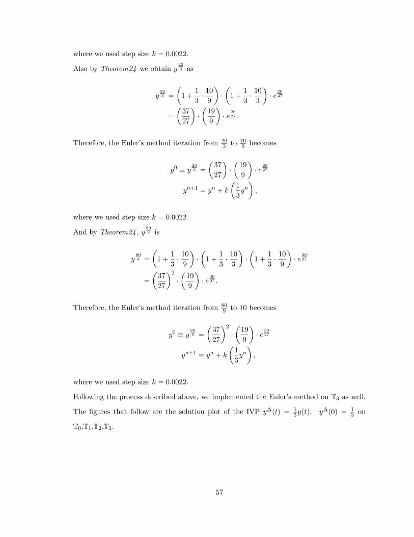
where we used step size k “ 0.0022.
Also by Theorem24 we obtain y203 as
y203 “
ˆ
1`1
3¨
10
9
˙
¨
ˆ
1`1
3¨
10
3
˙
¨ e2027
“
ˆ
37
27
˙
¨
ˆ
19
9
˙
¨ e2027 .
Therefore, the Euler’s method iteration from 203 to 70
9 becomes
y0 ” y203 “
ˆ
37
27
˙
¨
ˆ
19
9
˙
¨ e2027
yn`1 “ yn ` k
ˆ
1
3yn˙
,
where we used step size k “ 0.0022.
And by Theorem24 , y809 is
y809 “
ˆ
1`1
3¨
10
9
˙
¨
ˆ
1`1
3¨
10
3
˙
¨
ˆ
1`1
3¨
10
9
˙
¨ e2027
“
ˆ
37
27
˙2
¨
ˆ
19
9
˙
¨ e3027 .
Therefore, the Euler’s method iteration from 809 to 10 becomes
y0 ” y809 “
ˆ
37
27
˙2
¨
ˆ
19
9
˙
¨ e3027
yn`1 “ yn ` k
ˆ
1
3yn˙
,
where we used step size k “ 0.0022.
Following the process described above, we implemented the Euler’s method on T3 as well.
The figures that follow are the solution plot of the IVP y∆ptq “ 13yptq, y∆p0q “ 1
3 on
T0,T1,T2,T3.
57
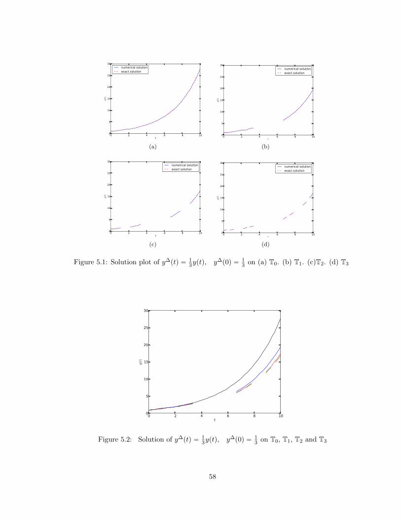
0 2 4 6 8 10t
0
5
10
15
20
25
30
y(t)
numerical solutionexact solution
(a)
0 2 4 6 8 10t
0
5
10
15
20
25
30
y(t)
numerical solutionexact solution
(b)
0 2 4 6 8 10t
0
5
10
15
20
25
30
y(t)
numerical solutionexact solution
(c)
0 2 4 6 8 10t
0
5
10
15
20
25
30
y(t)
numerical solutionexact solution
(d)
Figure 5.1: Solution plot of y∆ptq “ 13yptq, y∆p0q “ 1
3 on (a) T0. (b) T1. (c)T2. (d) T3
0 2 4 6 8 10t
0
5
10
15
20
25
30
y(t)
Figure 5.2: Solution of y∆ptq “ 13yptq, y∆p0q “ 1
3 on T0, T1, T2 and T3
58
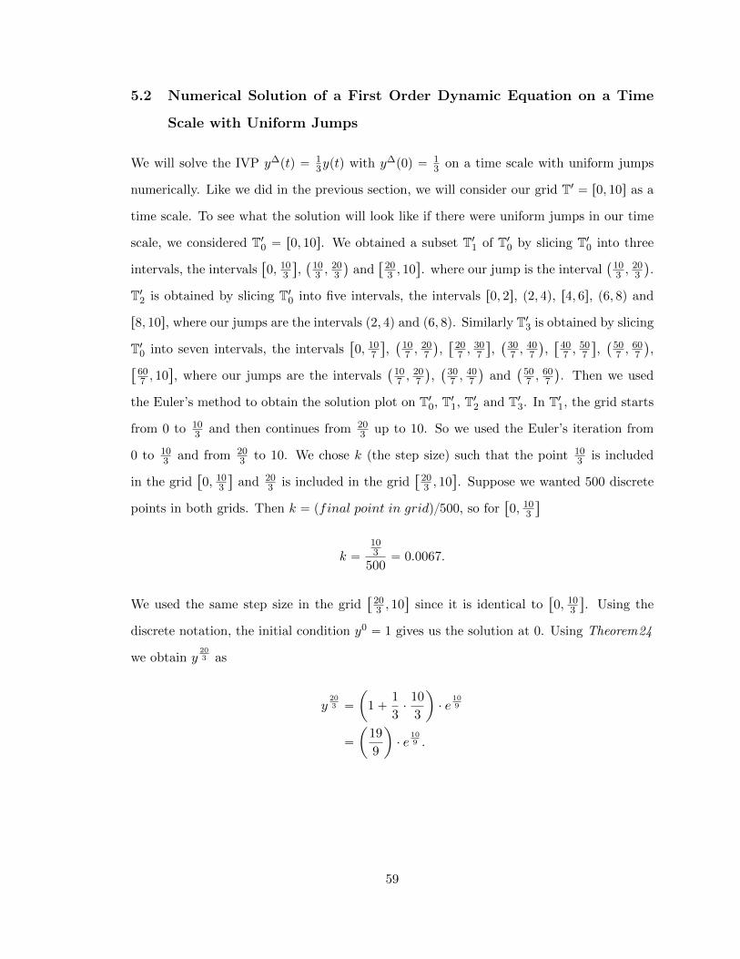
5.2 Numerical Solution of a First Order Dynamic Equation on a Time
Scale with Uniform Jumps
We will solve the IVP y∆ptq “ 13yptq with y∆p0q “ 1
3 on a time scale with uniform jumps
numerically. Like we did in the previous section, we will consider our grid T1 “ r0, 10s as a
time scale. To see what the solution will look like if there were uniform jumps in our time
scale, we considered T10 “ r0, 10s. We obtained a subset T11 of T10 by slicing T10 into three
intervals, the intervals“
0, 103
‰
,`
103 ,
203
˘
and“
203 , 10
‰
. where our jump is the interval`
103 ,
203
˘
.
T12 is obtained by slicing T10 into five intervals, the intervals r0, 2s, p2, 4q, r4, 6s, p6, 8q and
r8, 10s, where our jumps are the intervals p2, 4q and p6, 8q. Similarly T13 is obtained by slicing
T10 into seven intervals, the intervals“
0, 107
‰
,`
107 ,
207
˘
,“
207 ,
307
‰
,`
307 ,
407
˘
,“
407 ,
507
‰
,`
507 ,
607
˘
,“
607 , 10
‰
, where our jumps are the intervals`
107 ,
207
˘
,`
307 ,
407
˘
and`
507 ,
607
˘
. Then we used
the Euler’s method to obtain the solution plot on T10, T11, T12 and T13. In T11, the grid starts
from 0 to 103 and then continues from 20
3 up to 10. So we used the Euler’s iteration from
0 to 103 and from 20
3 to 10. We chose k (the step size) such that the point 103 is included
in the grid“
0, 103
‰
and 203 is included in the grid
“
203 , 10
‰
. Suppose we wanted 500 discrete
points in both grids. Then k “ pfinal point in gridq{500, so for“
0, 103
‰
k “103
500“ 0.0067.
We used the same step size in the grid“
203 , 10
‰
since it is identical to“
0, 103
‰
. Using the
discrete notation, the initial condition y0 “ 1 gives us the solution at 0. Using Theorem24
we obtain y203 as
y203 “
ˆ
1`1
3¨
10
3
˙
¨ e109
“
ˆ
19
9
˙
¨ e109 .
59

Therefore, the Euler’s method iteration from 203 in our grid becomes
y0 ” y203 “
ˆ
19
9
˙
¨ e109
yn`1 “ yn ` k
ˆ
1
3yn˙
.
Similarly in T12, the grid starts from 0 to 2, continues from 4 to 6 and from 8 to 10. So the
Euler’s iteration is used from 0 to 2, 4 to 6 and from 8 to 10. We chose k (the step size)
such that the point 2 is included in the grid r0, 2s, 4 and 6 are included in the grid r4, 6s
and 8 is included in the grid r8, 10s. Suppose we wanted 500 discrete points in the three
grids. Then k “ pfinal point in gridq{500, so for r0, 2s
k “2
500“ 0.004.
We used the same step size in the grid r4, 6s and r8, 10s since they are identical to r0, 2s.
Theorem24 also gives us y4 as
y4 “
ˆ
1`1
3¨ 2
˙
¨ e23
“
ˆ
5
3
˙
¨ e23
Therefore, the Euler’s method iteration from 4 to 6 becomes
y0 ” y4 “
ˆ
5
3
˙
¨ e23
yn`1 “ yn ` k
ˆ
1
3yn˙
,
60

where we used step size k “ 0.004.
Also by Theorem24 we obtain y8 as
y8 “
ˆ
1`1
3¨ 2
˙
¨
ˆ
1`1
3¨ 2
˙
¨ e43
“
ˆ
5
3
˙2
¨ e43 .
Therefore, the Euler’s method iteration from 8 to 10 becomes
y0 ” y8 “
ˆ
5
3
˙2
¨ e43
yn`1 “ yn ` k
ˆ
1
3yn˙
,
where we used step size k “ 0.004.
Following the process described above, we implemented the Euler’s method on T13 as well.
The figures that follow are the solution plots of the IVP y∆ptq “ 13yptq, y∆p0q “ 1
3 on
T10,T11,T12,T13.
61

0 2 4 6 8 10t
0
5
10
15
20
25
30
y(t)
numerical solutionexact solution
(a)
0 2 4 6 8 10t
0
5
10
15
20
25
30
y(t)
numerical solutionexact solution
(b)
0 2 4 6 8 10t
0
5
10
15
20
25
30
y(t)
numerical solutionexact solution
(c)
0 2 4 6 8 10t
0
5
10
15
20
25
30
y(t)
numerical solutionexact solution
(d)
Figure 5.3: Solution plot of y∆ptq “ 13yptq, y∆p0q “ 1
3 on (a)T10. (b) T11. (c) T12. (d) T13
0 2 4 6 8 10t
0
5
10
15
20
25
30
y(t)
Figure 5.4: Solution of y∆ptq “ 13yptq, y∆p0q “ 1
3 on T10, T11, T12 and T13
62

63
Appendix A
Thesis approval from IRB
64

Appendix B
Python code
# Solving DE on a time scale with no jump T = [0, 10]
# y’ = (1/3)*y(t)
# y(t) = exp((1/3)*t)
from pylab import *
N1 = 500 # k=0.01
def F(u,t):
return (1.0/3)*u
def exactSolution(t):
return exp((1.0*t)/3)
finalT = 10.0
y1 = zeros((N1,1))
tp1 = zeros((N1,1))
y1[0] = 1.0
65
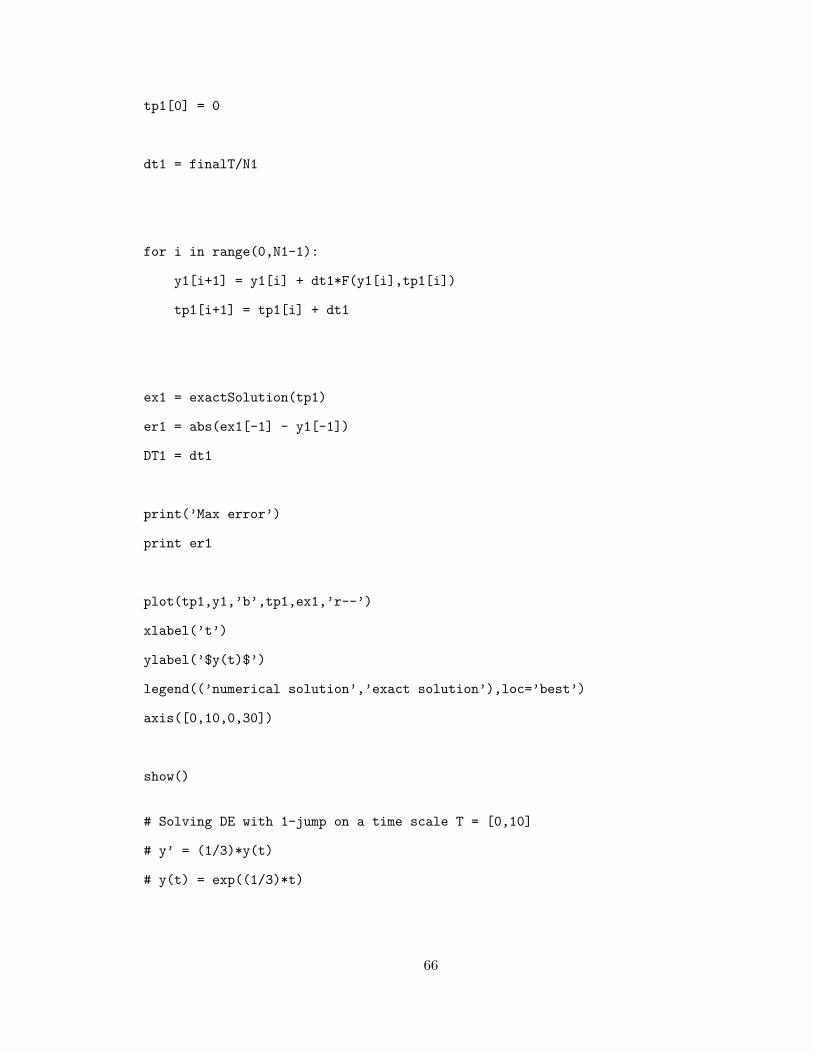
tp1[0] = 0
dt1 = finalT/N1
for i in range(0,N1-1):
y1[i+1] = y1[i] + dt1*F(y1[i],tp1[i])
tp1[i+1] = tp1[i] + dt1
ex1 = exactSolution(tp1)
er1 = abs(ex1[-1] - y1[-1])
DT1 = dt1
print(’Max error’)
print er1
plot(tp1,y1,’b’,tp1,ex1,’r--’)
xlabel(’t’)
ylabel(’$y(t)$’)
legend((’numerical solution’,’exact solution’),loc=’best’)
axis([0,10,0,30])
show()
# Solving DE with 1-jump on a time scale T = [0,10]
# y’ = (1/3)*y(t)
# y(t) = exp((1/3)*t)
66

from pylab import *
y0 = 1.0
N1 = 500 # k=0.01
def F(u,t):
return (1.0/3)*u
def exactSolution1(t):
return exp((1.0*t)/3)
def exactSolution2(t):
return (19.0/9)*exp(10.0/9)*exp((t-(20.0/3))/3)
finalT1 = 10.0/3
y1 = zeros((N1,1))
y2 = zeros((N1,1))
tp1 = zeros((N1,1))
tp2 = zeros((N1,1))
y1[0] = 1.0
y2[0] = (19.0/9)*exp(10.0/9)
tp1[0] = 0
tp2[0] = 20.0/3
dt1 = finalT1/N1
67
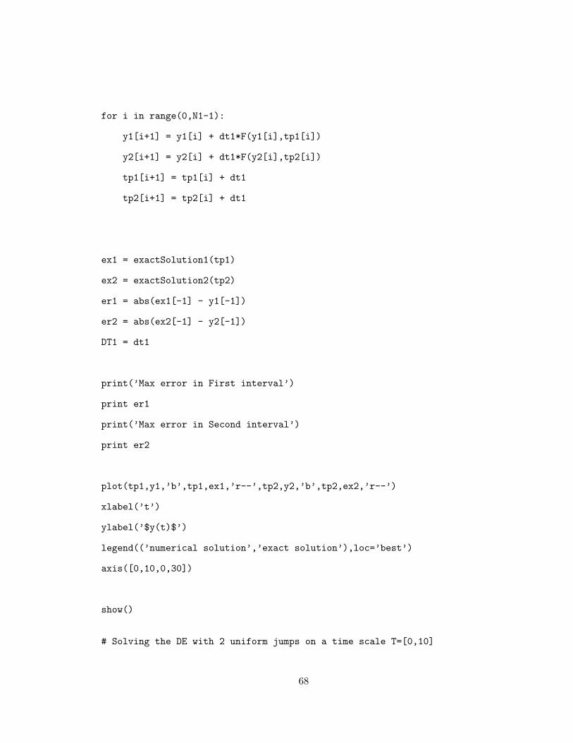
for i in range(0,N1-1):
y1[i+1] = y1[i] + dt1*F(y1[i],tp1[i])
y2[i+1] = y2[i] + dt1*F(y2[i],tp2[i])
tp1[i+1] = tp1[i] + dt1
tp2[i+1] = tp2[i] + dt1
ex1 = exactSolution1(tp1)
ex2 = exactSolution2(tp2)
er1 = abs(ex1[-1] - y1[-1])
er2 = abs(ex2[-1] - y2[-1])
DT1 = dt1
print(’Max error in First interval’)
print er1
print(’Max error in Second interval’)
print er2
plot(tp1,y1,’b’,tp1,ex1,’r--’,tp2,y2,’b’,tp2,ex2,’r--’)
xlabel(’t’)
ylabel(’$y(t)$’)
legend((’numerical solution’,’exact solution’),loc=’best’)
axis([0,10,0,30])
show()
# Solving the DE with 2 uniform jumps on a time scale T=[0,10]
68
# y’ = (1/3)*y(t)
# y(t) = exp((1/3)*t)
from pylab import *
N1 = 500 # k=0.01
def F(u,t):
return (1.0/3)*u
def exactSolution1(t):
return exp((1.0*t)/3)
def exactSolution2(t):
return (5.0/3)*exp(2.0/3)*exp((t-4.0)/3)
def exactSolution3(t):
return ((5.0/3)**2)*exp(4.0/3)*exp((t-(8.0))/3)
finalT1 = 2.0
y1 = zeros((N1,1))
y2 = zeros((N1,1))
y3 = zeros((N1,1))
tp1 = zeros((N1,1))
tp2 = zeros((N1,1))
tp3 = zeros((N1,1))
69

y1[0] = 1.0
y2[0] = (5.0/3)*exp(2.0/3)
y3[0] = ((5.0/3)**2)*exp(4.0/3)
tp1[0] = 0
tp2[0] = 4.0
tp3[0] = 8.0
dt1 = finalT1/N1
for i in range(0,N1-1):
y1[i+1] = y1[i] + dt1*F(y1[i],tp1[i])
y2[i+1] = y2[i] + dt1*F(y2[i],tp2[i])
y3[i+1] = y3[i] + dt1*F(y3[i],tp3[i])
tp1[i+1] = tp1[i] + dt1
tp2[i+1] = tp2[i] + dt1
tp3[i+1] = tp3[i] + dt1
ex1 = exactSolution1(tp1)
ex2 = exactSolution2(tp2)
ex3 = exactSolution3(tp3)
er1 = abs(ex1[-1] - y1[-1])
er2 = abs(ex2[-1] - y2[-1])
er3 = abs(ex3[-1] - y3[-1])
DT1 = dt1
print(’Max error in First interval’)
70
print er1
print(’Max error in Second interval’)
print er2
print(’Max error in Third interval’)
print er3
plot(tp1,y1,’b’,tp1,ex1,’r--’,tp2,y2,’b’,tp2,ex2,’r--’,tp3,y3,’b’,tp3,ex3,’r--’)
xlabel(’t’)
ylabel(’$y(t)$’)
legend((’numerical solution’,’exact solution’),loc=’best’)
axis([0,10,0,30])
show()
# Solving the DE with 3 uniform jumps on T = [0,10]
# y’ = (1/3)*y(t)
# y(t) = exp((1/3)*t)
from pylab import *
N1 = 500 # k=0.01
def F(u,t):
return (1.0/3)*u
def exactSolution1(t):
return exp((1.0*t)/3)
def exactSolution2(t):
71
return (31.0/21)*exp(10.0/21)*exp((t-(20.0/7))/3)
def exactSolution3(t):
return ((31.0/21)**2)*exp(20.0/21)*exp((t-(40.0/7))/3)
def exactSolution4(t):
return ((31.0/21)**3)*exp(30.0/21)*exp((t-(60.0/7))/3)
finalT1 = 10.0/7
y1 = zeros((N1,1))
y2 = zeros((N1,1))
y3 = zeros((N1,1))
y4 = zeros((N1,1))
tp1 = zeros((N1,1))
tp2 = zeros((N1,1))
tp3 = zeros((N1,1))
tp4 = zeros((N1,1))
y1[0] = 1.0
y2[0] = (31.0/21)*exp(10.0/21)
y3[0] = ((31.0/21)**2)*exp(20.0/21)
y4[0] = ((31.0/21)**3)*exp(30.0/21)
tp1[0] = 0
tp2[0] = 20.0/7
tp3[0] = 40.0/7
tp4[0] = 60.0/7
72

dt1 = finalT1/N1
for i in range(0,N1-1):
y1[i+1] = y1[i] + dt1*F(y1[i],tp1[i])
y2[i+1] = y2[i] + dt1*F(y2[i],tp2[i])
y3[i+1] = y3[i] + dt1*F(y3[i],tp3[i])
y4[i+1] = y4[i] + dt1*F(y4[i],tp4[i])
tp1[i+1] = tp1[i] + dt1
tp2[i+1] = tp2[i] + dt1
tp3[i+1] = tp3[i] + dt1
tp4[i+1] = tp4[i] + dt1
ex1 = exactSolution1(tp1)
ex2 = exactSolution2(tp2)
ex3 = exactSolution3(tp3)
ex4 = exactSolution4(tp4)
er1 = abs(ex1[-1] - y1[-1])
er2 = abs(ex2[-1] - y2[-1])
er3 = abs(ex3[-1] - y3[-1])
er4 = abs(ex4[-1] - y4[-1])
DT1 = dt1
print(’Max error in First interval’)
print er1
print(’Max error in Second interval’)
73
print er2
print(’Max error in Third interval’)
print er3
print(’Max error in Fourth interval’)
print er4
plot(tp1,y1,’b’,tp1,ex1,’r--’,tp2,y2,’b’,tp2,ex2,’r--’,tp3,y3,’b’,tp3,ex3,’r--’,\-
tp4,y4,’b’,tp4,ex4,’r--’)
xlabel(’t’)
ylabel(’$y(t)$’)
legend((’numerical solution’,’exact solution’),loc=’best’)
axis([0,10,0,30])
show()
74

REFERENCES
[1] R. Agarwal, M. Bohner, D. O’Regan, and A. Peterson, Dynamic equations on timescales: a survey, Journal of Computational and Applied Mathematics Volume 141(2001), Pages 1 – 26.
[2] M. Bohner and A. Peterson, Dynamic equations on times scales: An introduction withapplications, Birkh:auser, Boston, 2001.
[3] , First course on dynamic equations on time scales, Preliminary final version for2nd edition of Dynamic Equation on Time Scales (2009).
[4] J. Crank, The differential analyzer, Longmans, Green, & Co., 1947.
[5] W. Kelley and A. Peterson, Difference equations, 2nd ed., Academic Press, 2001.
[6] Bonita A. Lawrence, Sher Chhetri, Richard Merrit, Daniel Olumoyin, and Molly Peter-son, Solutions of differential equations on time scales created by mechanical integration,Texas A & M, Kingsville (December, 2012).
75
Kayode Daniel Olumoyin
Born December 29, 1985 in Lagos, Nigeria
Education
• Master of Arts. Marshall University, May 2013. Thesis Advisor: Dr. Bonita Lawrence
• Bachelor of Science. University of Agriculture, Abeokuta. January 2009, Second ClassUpper.
Awards
1. Winifred O. Stone Presidential Graduate Scholarship Award for Diversity Enhance-ment for 2013-2014 academic year, Bowling Green State University.
2. Won First Position (University Ranking) and Second Prize winner (Individual rank-ing) at the National Mathematics Competition for University Students (NAMCUS2008). This is an annual Mathematics Competition held in Nigeria at the NationalMathematical Centre, Abuja. Each University is represented by a team of four stu-dents.
Publication
1. Solutions of Dynamic Equations on Time Scales with Jumps. Master’s thesis, MarshallUniversity, May 2013.
Conference Presentation
1. Generalization of First Order Linear Differential and Difference Equations. 40thAnnual Mathematics and Statistics Conference, Miami University, Oxford, OH,(September 2012).
Teaching Experience Marshall University, Huntington, WV
1. Graduate Teaching Assistant (Fall 2011, Spring 2012, Fall 2012, Spring 2013):Worked in the Differential Analyzer Lab (Spring 2012, Fall 2012 and Spring 2013)
2. Introductory Statistics (MTH 225; Fall 2011, Summer 2012):Responsible for preparing and delivering lectures, grading examination, homework,and assigning final grades.
3. Mathematics Skills II (MTH 099; Fall 2012):Responsible for preparing and delivering lectures, grading examination, homework,and assigning final grades.
4. College Algebra (MTH 127; Spring 2013):Responsible for preparing and delivering lectures, grading examination, quizzes, andassigning final grades.
National Youth Service, Borno, Nigeria
1. Headmaster, Bayo Foundation/NYSC Nursery School, Bayo, Borno (January to July2010). The National Youth Service is a volunteer programme for College graduates.I served as the Headmaster at the above school. I had 10 other volunteers as memberof staff. My duties range from administrative, to teaching as well as staff welfare.
76

2. Mathematics teacher, UBE Junior School, Bayo, Borno (August 2009 to January2010). Responsible for teaching, grading and coaching the Mathematics Club.
Conference Attended
1. The 31st Southeastern-Atlantic Regional Conference on Differential Equations, Geor-gia Southern University, September 2011.
2. 96th Annual Meeting of the Mathematical Association of America, Ohio Section,Spring 2012, Xavier University, Cincinnati, Ohio, April 2012.
3. 40th Annual Mathematics and Statistics Conference, Miami University, Oxford, OH,September 2012.
Professional Membership
Pi Mu Epsilon (West Virginia Beta chapter)
Programming & Software Experience
Python, GAP 4, LATEXtypesetting, Microsoft Office
Coursework
(Marshall University):Mordern Algebra (2 semesters), Probability and Statistics (2 semesters),Advanced Calculus (2 semesters), Advanced Number Theory, Complex Variables I, Numer-ical Analysis, Numerical Partial Differential Equations.pending(Time Scales Calculus, Complex Variables II, Advanced Diffrential Equation).
(UNAAB):Algebra, Vectors and Geometry, Calculus and Trigonometry, Mechanics, Ab-stract Algebra(2 semesters), Real Analysis(2 semesters),Linear Algebra, Ordinary Differ-ential Equations, General Statistics, Statistical Inference, Probability, Data structure andAlgorithm, Vector and Tensors Analysis,Theory of Modules, Metric Spaces, General Topol-ogy, Advanced Algebra(2 semesters) Partial Differential Equations
77