solutions - eth z...page 4 system modeling description: consider the state-space representation _x=...
TRANSCRIPT

23.01.2019
System Modeling (151-0573-00) Dr. G. Ducard, M. Salazar
Solutions
Exam Duration: 120 min + 15 min reading time at the beginning.
Number of Questions: 40 (50 points total)
Rating: The number of achievable points is indicated for each ques-
tion.
Points are only awarded for completely correct solutions.
Multiple-choice questions have only one correct solution.
Permitted aids: 20 A4-sheets (= 40 pages)
No additional aids or electronic devices (no calculators, no
smartphones, etc.)
The assistants are not allowed to help.
Important: Only the given end result is evaluated.
Write down your solutions at the indicated locations only.

Page 2 System Modeling
Topic: Relevant Dynamics
Description: Consider the exhaust path of a Diesel engine as shown in Figure 1. It consistsof the exhaust manifold (EM), the turbine (T), the exhaust pipe (EP), and the aftertreatmentsystem (ATS). The temperature of the exhaust gas can be measured at the various positionsindicated by the arrows. Furthermore, the engine coolant temperature is recorded, which isrepresentative of the temperature of the engine block. Figure 2 shows measurements of thesetemperatures during a sudden increase and decrease of the engine power.
ϑATS,down
EM
T
ATS
ϑATS,upϑEM
ϑcoolant
EP
Engineblock
Figure 1: Diesel engine exhaust path and aftertreatment system.
80
85
90
95
ϑco
olant
[◦C
]
350
450
550
ϑEM
[◦C
]
60 80 100 120320
360
400
Time [s]
ϑATS,up
[◦C
]
60 80 100 120320
360
400
Time [s]
ϑATS,down
[◦C
]
Figure 2: Temperatures during a sudden increase and decrease of the engine power.
For the following two questions, assume that we want to derive a model for the temperature ofthe ATS. For each component, indicate with a cross (7) what type of model for its temperatureis most suitable.
Q1 (1 point)
Component Dynamic Algebraic Static
Engine block 7
Exhaust manifold 7
Explanation: The engine block temperature dynamics represented by ϑcoolant are very

System Modeling Page 3
slow with respect to the other signals. Conversely, the exhaust manifold temperatureϑEM changes almost instantaneously.
Q2 (1 point)
Component Dynamic Algebraic Static
Exhaust pipe 7
ATS 7
Explanation: Both the temperatures before and after the ATS have a non-negligibledynamic behaviour.

Page 4 System Modeling
Description: Consider the state-space representation x = Ax+Bu of a dynamic system with
A =
−1 1 2−4 −2 020 0 −20
B =
1100
.
Applying an input step to this system reveals that x3 can be assumed to be algebraic. Therefore,we can neglect the dynamics of the third state and simplify the system by incorporating theresulting algebraic equation into the dynamics of the two other states.
Q3 (1 point) Write down the system matrix A and the input matrix B of the simplifiedsystem.
Solution:
A =
[1 1−4 −2
]B =
[1
10
]Explanation:The given state-space description reads:
d
dtx1 = −x1 + x2 + 2 · x3 + u
d
dtx2 = −4 · x1 − 2 · x2 + 10 · u
d
dtx3 = 20 · x1 − 20 · x3
Neglecting the dynamics of the third state, we get: 0 =d
dtx3 = 20·(x1−x3)⇒
x3 = x1. Incorporating this relation into the state equations for the first andsecond state yields:
d
dtx1 = −x1 + x2 + 2 · x1 + u = x1 + x2 + u
d
dtx2 = −4 · x1 − 2 · x2 + 10 · u
The matrices for the simplified system with state vector x = (x1, x2)> read
A =
[1 1−4 −2
]B =
[1
10
].

System Modeling Page 5
Topic: Causality Diagram
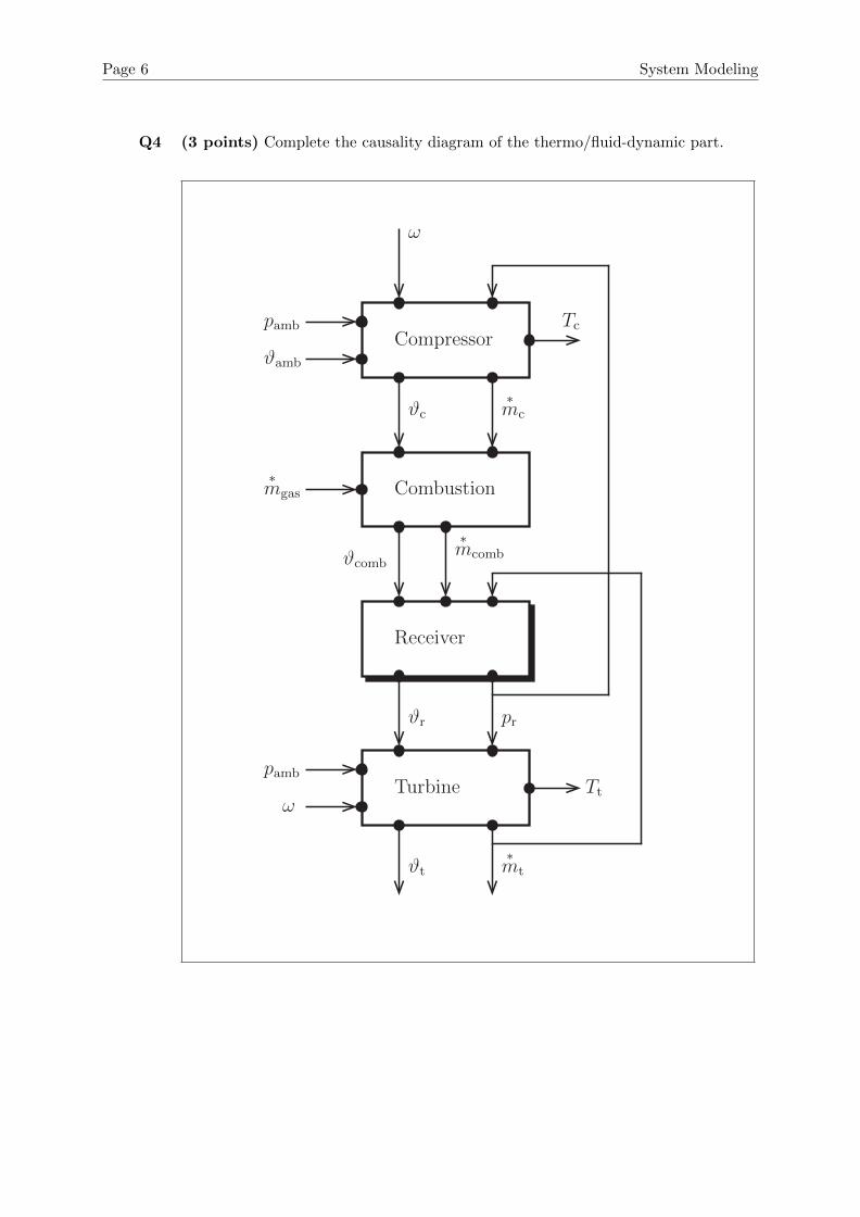
Description: Figure 3 shows a simplified representation of a gas turbine power plant. Airenters the compressor at ambient (amb) conditions. Downstream of the compressor, naturalgas is injected and ignited. The combustion, assumed to be an isobaric process, increasesthe temperature of the air/fuel mixture. The hot gases then enter a receiver that is perfectlyinsulated. Subsequently, they exit the receiver and flow through the turbine. The shaft of thecompressor and turbine is connected to a generator to produce electric power.
pamb
pamb
ϑamb
∗mgas
Compressor Turbine
ω
GeneratorUind
I
Combustion
Receiver
Air
Figure 3: Gas turbine power plant.
The system is split up as follows: on the one hand, the thermo/fluid-dynamic part, and on theother hand, the mechanical/electric part. Your task is to derive and draw the causality diagramfor both parts.
The variables you can use are listed in Table 1. Some of these physical quantities are inputsand/or outputs of multiple components. Use the subscripts defined in Table 2 for the outputsignals of each component/block.
Variable Symbol
Pressure p
Temperature ϑ
Massflow∗m
Torque T
Rotational speed ω
Electric current I
Induced voltage Uind
Table 1
Component Subscript
Compressor c
Combustion comb
Receiver r
Turbine t
Generator g
Table 2
For connecting the blocks using lines/arrows, use the top and left side for inputs, and thebottom and right side for outputs. The dots on each side of each block indicate the amountand location of lines/arrows that should be connected. Recall that shaded blocks are used fordynamic subsystems.
Page 6 System Modeling
Q4 (3 points) Complete the causality diagram of the thermo/fluid-dynamic part.
Compressor
Combustion
Turbine
∗mgas
Tt
ϑcomb
∗mc
pamb
Receiver
ϑamb
pamb
ω
ϑc
ω
ϑr pr
∗mtϑt
Tc
∗mcomb
System Modeling Page 7
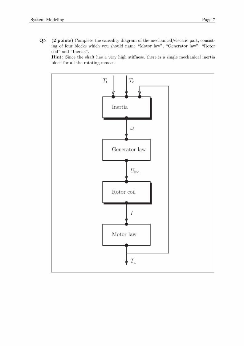
Q5 (2 points) Complete the causality diagram of the mechanical/electric part, consist-ing of four blocks which you should name “Motor law”, “Generator law”, “Rotorcoil” and “Inertia”.Hint: Since the shaft has a very high stiffness, there is a single mechanical inertiablock for all the rotating masses.
Tt Tc
Tg
Inertia
Generator law
Motor law
Rotor coil
ω
Uind
I

Page 8 System Modeling
Topic: Mechanics
Description: Consider the piston of an internal combustion engine as shown in Figure 4. Thepiston with mass m is connected by a rigid massless rod to a crankshaft with rotational inertia Θ.This mechanical system translates the longitudinal motion of the piston to a rotational motionof the crankshaft. The rotation of the crankshaft is described by the coordinate ϕ, whereas theposition of the piston is described by the coordinate x. The position of the piston is related tothe position of the crankshaft by
x = r
(1− cos(ϕ) +
1
2
r
lsin2(ϕ)
).
Assume that the piston slides without friction across the cylinder surface.
crankshaft
piston
working gas
rod
m
Θ
x
ϕ
r
l
cylinder
Figure 4: Sketch of the piston and the equivalent mechanical model.
Q6 (1 point) Is q = x a suitable choice of generalized coordinate?
� Yes.
� No.
Explanation: The sole coordinate x is ambiguous, as one cannot tell whether thepiston is moving upwards or downwards.
Q7 (1 point) Is the system holonomic?
� Yes.
� No.
Explanation: The constraint is holonomic, since it can be formulated with positioncoordinates only.

System Modeling Page 9
Q8 (2 points) Now let q = ϕ. Calculate the kinetic energy of the system.
T (q, q) =1
2mr2
(sin(q)q +
r
lsin(q) cos(q)q
)2+
1
2Θq2
Explanation:The kinetic energy of the system consists of the translational kinetic energyof the piston Tpiston and the rotational kinetic energy of the flywheel Trot.Therefore, the total kinetic energy T reads
T =1
2mx2 +
1
2Θϕ2.
Using the constraint from the previous page, x is eliminated from the equation.The derivative of x with respect to time reads
x = r(
sin(ϕ)ϕ+r
lsin(ϕ)cos(ϕ)ϕ
).
Assuming an isentropic compression and expansion of the working gas inside the cylinder withisentropic coefficient γ, the gas-spring force can be derived as
Fp(x) = C1
((1− C2x)γ − 1
),
where C1 and C2 are constants.
Q9 (1 point) Is Fp a conservative force?
� Yes.
� No.
� No conclusion possible.
Explanation:In general, a conservative force F can be represented as the gradient of a potentialfunction U(q) as
F = −∂U∂q
>.
In our one-dimensional case, this translates to
Fp = −∂U∂x
.
Since Fp is a sole function of position and it is integrable, we can construct itspotential function U . Therefore, it is a conservative force.
Page 10 System Modeling
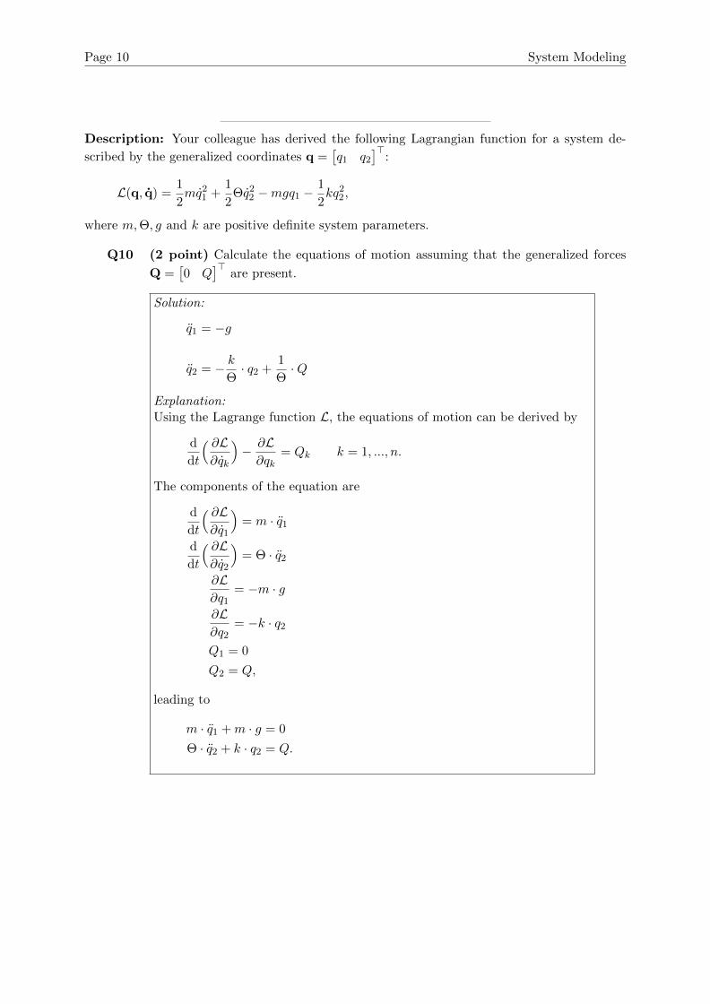
Description: Your colleague has derived the following Lagrangian function for a system de-
scribed by the generalized coordinates q =[q1 q2
]>:
L(q, q) =1
2mq21 +
1
2Θq22 −mgq1 −
1
2kq22,
where m,Θ, g and k are positive definite system parameters.
Q10 (2 point) Calculate the equations of motion assuming that the generalized forces
Q =[0 Q
]>are present.
Solution:
q1 = −g
q2 = − kΘ· q2 +
1
Θ·Q
Explanation:Using the Lagrange function L, the equations of motion can be derived by
d
dt
( ∂L∂qk
)− ∂L∂qk
= Qk k = 1, ..., n.
The components of the equation are
d
dt
( ∂L∂q1
)= m · q1
d
dt
( ∂L∂q2
)= Θ · q2
∂L∂q1
= −m · g
∂L∂q2
= −k · q2
Q1 = 0
Q2 = Q,
leading to
m · q1 +m · g = 0
Θ · q2 + k · q2 = Q.

System Modeling Page 11
Topic: Hydraulics
Description: Consider the simultaneous filling and emptying of the reservoir shown in Figure 5.The cross-sectional area of the reservoir is A. The water has a constant density ρ and is suppliedat a total pressure ps > pamb. The ambient pressure is denoted by pamb. The water level inthe reservoir is h. The lift arm connected to the float has length L (this is also the maximumfilling height) and an angle α with respect to its vertical position (α = 0 when the reservoiris completely empty). The lift arm’s pivot point is connected through gears to the inlet valve,thereby regulating the supply of water. The area of the inlet valve is Ain(α), whereas theoutlet has a constant area Aout. The inlet valve can be modeled using the model of a valve forincompressible flows with cd = 1. Assume a frictionless flow in the tank and in the outlet pipe.Finally, g denotes the gravitational acceleration.
m, ρ
L
L
pspamb
pamb
Aout
Ain(α)
α
A
g
h
Figure 5: Water reservoir schematic.
Q11 (1 point) Derive an algebraic expression for the massflow into the reservoir, depend-ing on the angle α and (some of) the variables mentioned in the description.Hint: Treat Ain(α) as a given function.
Solution:
∗min(α) = Ain(α) ·
√2 · ρ · (ps − pamb)
Explanation: The solution follows from the valve flow equation for an incom-pressible flow and cd = 1.
Page 12 System Modeling
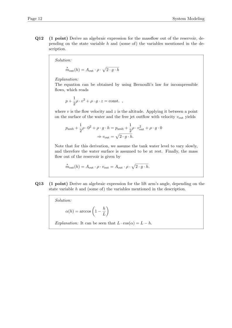
Q12 (1 point) Derive an algebraic expression for the massflow out of the reservoir, de-pending on the state variable h and (some of) the variables mentioned in the de-scription.
Solution:
∗mout(h) = Aout · ρ ·
√2 · g · h
Explanation:The equation can be obtained by using Bernoulli’s law for incompressibleflows, which reads
p+1
2ρ · v2 + ρ · g · z = const. ,
where v is the flow velocity and z is the altitude. Applying it between a pointon the surface of the water and the free jet outflow with velocity vout yields
pamb +1
2ρ · 02 + ρ · g · h = pamb +
1
2ρ · v2out + ρ · g · 0
⇒ vout =√
2 · g · h.
Note that for this derivation, we assume the tank water level to vary slowly,and therefore the water surface is assumed to be at rest. Finally, the massflow out of the reservoir is given by
∗mout(h) = Aout · ρ · vout = Aout · ρ ·
√2 · g · h.
Q13 (1 point) Derive an algebraic expression for the lift arm’s angle, depending on thestate variable h and (some of) the variables mentioned in the description.
Solution:
α(h) = arccos
(1− h
L
)Explanation: It can be seen that L · cos(α) = L− h.

System Modeling Page 13
Topic: Electrical Circuits
Description: Figure 6 shows an electrical circuit where an outgoing voltage Uout and currentI are induced by the input voltage Uin.
C
R
L
Uin Uout
UC
UL
I
UR
Figure 6: Sketch of an electrical circuit.
Symbol Description Unit
R Ohmic resistance V A−1
C Capacitance A s V−1
L Inductance V s A−1
Table 3: System parameters.

Page 14 System Modeling
Q14 (2 point) Let x =[I UC
]>, u = Uin and y = Uout. Write the system in the form
x = Ax+Bu
y = Cx+Du,
using the system parameters given in Table 3.
Solution:
A =
[−R/L −1/L1/C 0
]B =
[1/L
0
]C =
[R 0
]D = 0
Explanation:The state equations for the two dynamic elements, inductance and superca-pacitor, are given by
L · d
dtI = UL,
C · d
dtUC = I.
The state variables are coupled through Kirchhoff’s second law
Uin = UC + UR + UL,
where the ohmic voltage drop is UR = R · I. Using the last two equations andplugging them into the state equations yields
d
dtI =
1
L·(Uin − UC −R · I
)= −R
L· I − 1
L· UC +
1
L· Uin
d
dtUC =
1
C· I.
Finally, the output voltage is Uout = UR = R · I. This way, we can write thesystem in the state-space formulation.

System Modeling Page 15
Description: A supercapacitor is an electrostatic device that can be used to store electricalenergy. In comparison to a battery the supercapacitor allows for much higher current flows,however it is limited in the amount of electrical energy that can be stored. The maximal allowedvoltage for the supercapacitor is given by Umax. Useful energy storage can only be done if thevoltage does not drop below Umin = 1
2Umax. The supercapacitor has capacitance C.
Q15 (1 point) How much useful energy Euseful can be stored in a supercapacitor? Writeyour solution as a sole function of C and Umax.
Solution:
Euseful =1
2C · U2
max −1
2C ·(
1
2Umax
)2
=3
8C · U2
max
Explanation:The energy stored up to the minimal voltage 1
2C ·U2min is not usable. Therefore,
it has to be subtracted from the total energy 12C · U
2max.
Page 16 System Modeling
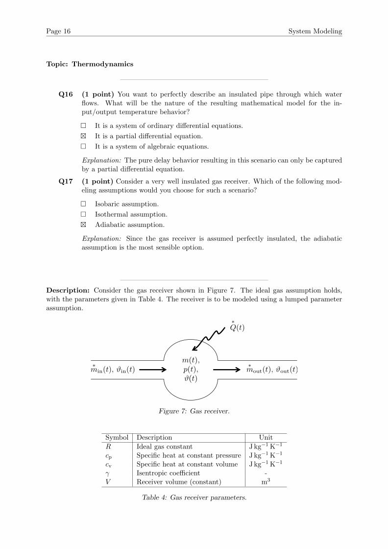
Topic: Thermodynamics
Q16 (1 point) You want to perfectly describe an insulated pipe through which waterflows. What will be the nature of the resulting mathematical model for the in-put/output temperature behavior?
� It is a system of ordinary differential equations.
� It is a partial differential equation.
� It is a system of algebraic equations.
Explanation: The pure delay behavior resulting in this scenario can only be capturedby a partial differential equation.
Q17 (1 point) Consider a very well insulated gas receiver. Which of the following mod-eling assumptions would you choose for such a scenario?
� Isobaric assumption.
� Isothermal assumption.
� Adiabatic assumption.
Explanation: Since the gas receiver is assumed perfectly insulated, the adiabaticassumption is the most sensible option.
Description: Consider the gas receiver shown in Figure 7. The ideal gas assumption holds,with the parameters given in Table 4. The receiver is to be modeled using a lumped parameterassumption.
Figure 7: Gas receiver.
Symbol Description Unit
R Ideal gas constant J kg−1 K−1
cp Specific heat at constant pressure J kg−1 K−1
cv Specific heat at constant volume J kg−1 K−1
γ Isentropic coefficient -V Receiver volume (constant) m3
Table 4: Gas receiver parameters.

System Modeling Page 17
Q18 (1 point) Which of the following statements is not implied by the lumped parameterassumption?
� The thermodynamic states are assumed to be the same all over the receiver.
�∗min =
∗mout.
� ϑout = ϑ(t), where ϑ(t) is the temperature in the receiver.
Explanation: In the lumped parameter assumption, the thermodynamic states (i.e.,pressures, temperatures, composition, etc.) are assumed to be the same all over thereceiver volume. It also requires that the outflowing gas has the same temperature asthe gas inside the receiver. However, the assumption does not require that inflowingand outflowing mass flows are equal.
Q19 (1 point) Now assume that there is no outflow, i.e.,∗mout(t) = 0 ∀t, and that the
incoming mass flow∗min and temperature ϑin are constant. The receiver could be
modeled using either an adiabatic or an isothermal assumption. Mark the correctending for the following sentence:
The rate at which pressure increases
� is identical for the isothermal and adiabatic assumptions.
� is faster for the isothermal assumption.
� is faster for the adiabatic assumption.
Explanation: One needs to compare the differential equations for the pressure p(t).
For the adiabatic assumption, the equation reads (remember,∗mout = 0):
d
dtp(t) =
γ ·RV· ∗min · ϑin
For the isothermal assumption, the equation reads:
d
dtp(t) =
R
V· ∗min · ϑin
Since γ > 1, the pressure increase rate is faster for the adiabatic assumption.

Page 18 System Modeling
Topic: Isenthalpic Throttle
Description: For deep scuba diving the gas composition heliox, containing a mixture of heliumand oxygen, is used. Heliox is assumed to be an ideal gas with isentropic coefficient γ = 1.5.Before the next dive trip, the diving bottle is filled with heliox up to a pressure of 200 bar. Due
to aging of the valve, a leakage mass flow∗m is present and the diving bottle loses gas slowly. A
sketch of the bottle is shown in Figure 8. Assume an isenthalpic throttle, an ambient pressurepamb = 1 bar and that the heliox in the bottle has the constant temperature ϑb = ϑamb.
pb,ϑb pamb,ϑambpb
ϑb
pamb
ϑamb
∗m
diving bottle
throttle
Figure 8: Sketch of a diving bottle.
Symbol Description Unit
Vb Bottle volume mϑb Heliox temperature in diving bottle KR Ideal gas constant for heliox J kg−1 K−1
γ Isentropic coefficient –Aleak Leakage area of valve m2
cd Discharge coefficient of the valve –
Table 5: System parameters for diving bottle.
System Modeling Page 19
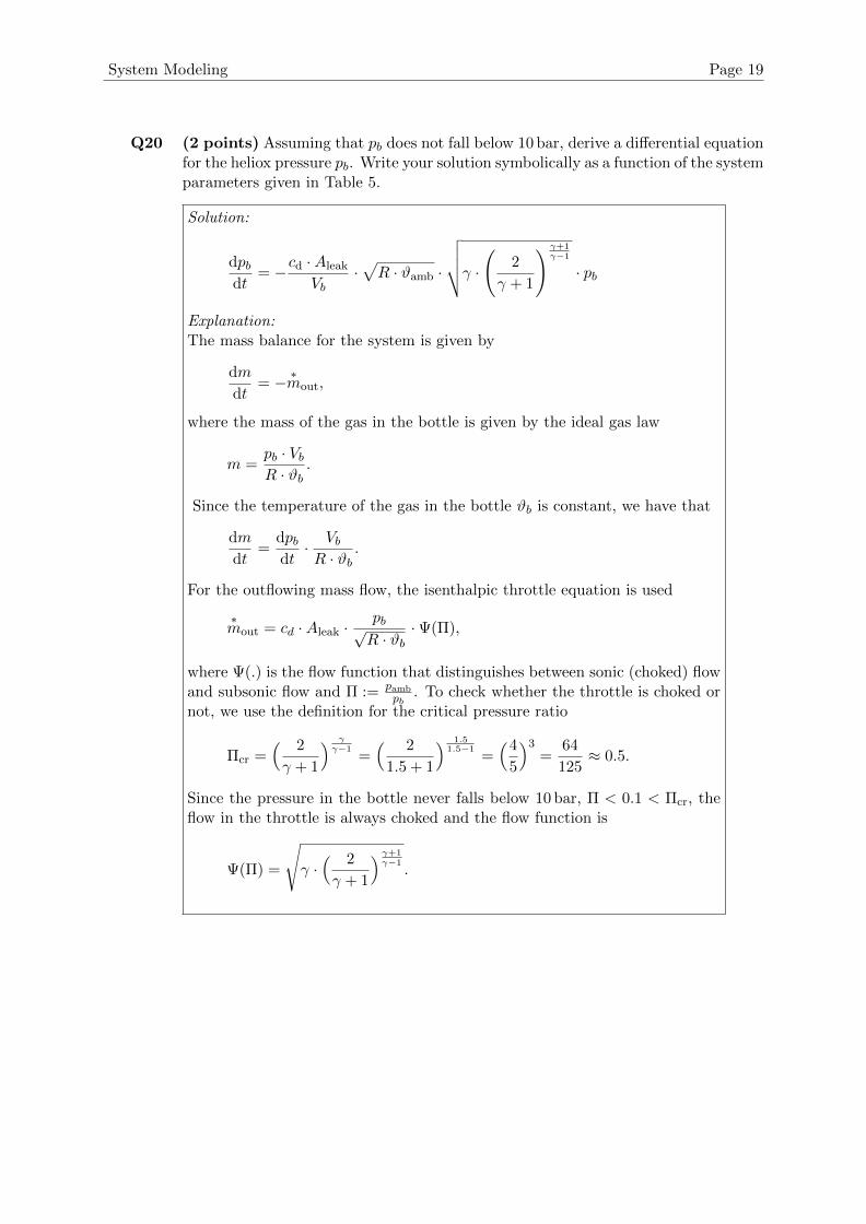
Q20 (2 points) Assuming that pb does not fall below 10 bar, derive a differential equationfor the heliox pressure pb. Write your solution symbolically as a function of the systemparameters given in Table 5.
Solution:
dpbdt
= −cd ·Aleak
Vb·√R · ϑamb ·
√√√√γ ·
(2
γ + 1
) γ+1γ−1
· pb
Explanation:The mass balance for the system is given by
dm
dt= − ∗mout,
where the mass of the gas in the bottle is given by the ideal gas law
m =pb · VbR · ϑb
.
Since the temperature of the gas in the bottle ϑb is constant, we have that
dm
dt=
dpbdt· VbR · ϑb
.
For the outflowing mass flow, the isenthalpic throttle equation is used
∗mout = cd ·Aleak ·
pb√R · ϑb
·Ψ(Π),
where Ψ(.) is the flow function that distinguishes between sonic (choked) flowand subsonic flow and Π := pamb
pb. To check whether the throttle is choked or
not, we use the definition for the critical pressure ratio
Πcr =( 2
γ + 1
) γγ−1
=( 2
1.5 + 1
) 1.51.5−1
=(4
5
)3=
64
125≈ 0.5.
Since the pressure in the bottle never falls below 10 bar, Π < 0.1 < Πcr, theflow in the throttle is always choked and the flow function is
Ψ(Π) =
√γ ·( 2
γ + 1
) γ+1γ−1
.

Page 20 System Modeling
After a successful dive with your colleagues, the bottle shows a remaining pressure of 3 bar attime t0. Since the valve of the diving bottle still exhibits leakage, you expect the bottle to becompletely empty for the next dive trip.
t
∗m(t)
t
∗m(t)
t
∗m(t)
t
∗m(t)
tt0
t0 t0
t0
I
III
II
IV
Figure 9: Different mass flow profiles.
Q21 (1 point) Looking at the different mass flow profiles in Figure 9, what will the
leakage mass flow∗m(t) look like over time?
� I
� II
� III
� IV
Explanation:To answer this question, we have to use the isenthalpic throttle equation
∗m = cd ·Aleak ·
pb√R · ϑb
·Ψ(Π), Ψ(Π) =
√γ ·(
2γ+1
) γ+1γ−1
Π < Πcr
Π1γ ·√
2γγ−1 ·
(1−Π
γ−1γ
)Π ≥ Πcr
and the fact that ϑb remains constant. At the beginning, the throttle is choked.The flow becomes subsonic once the pressure ratio Π becomes larger than the criticalpressure ratio Πcr. The first solution can be excluded due to the constant outflow atthe beginning implying the pressure pb being constant, which is unreasonable. Thesecond solution is unreasonable since there is no change in the behaviour of the flow.The third solution is unreasonable, since the outflow cannot increase. By exclusionthe fourth solution is the correct answer.
System Modeling Page 21
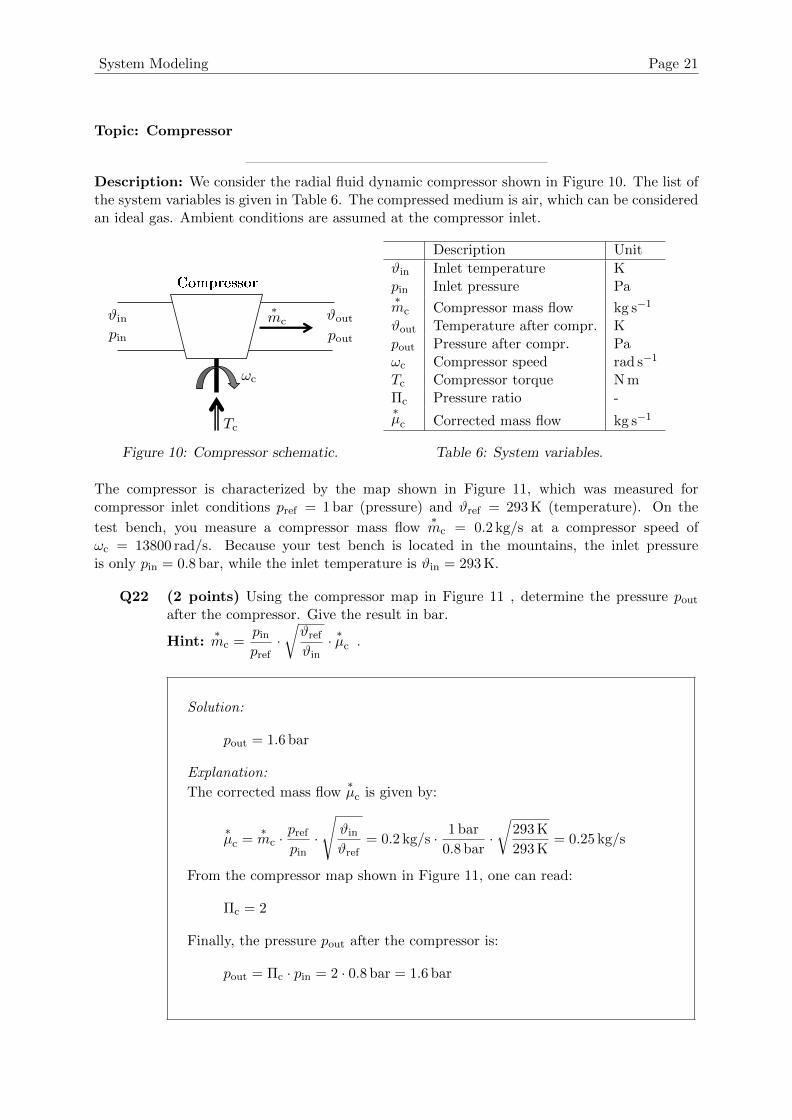
Topic: Compressor
Description: We consider the radial fluid dynamic compressor shown in Figure 10. The list ofthe system variables is given in Table 6. The compressed medium is air, which can be consideredan ideal gas. Ambient conditions are assumed at the compressor inlet.
Figure 10: Compressor schematic.
Description Unit
ϑin Inlet temperature Kpin Inlet pressure Pa∗mc Compressor mass flow kg s−1
ϑout Temperature after compr. Kpout Pressure after compr. Paωc Compressor speed rad s−1
Tc Compressor torque N mΠc Pressure ratio -∗µc Corrected mass flow kg s−1
Table 6: System variables.
The compressor is characterized by the map shown in Figure 11, which was measured forcompressor inlet conditions pref = 1 bar (pressure) and ϑref = 293 K (temperature). On the
test bench, you measure a compressor mass flow∗mc = 0.2 kg/s at a compressor speed of
ωc = 13800 rad/s. Because your test bench is located in the mountains, the inlet pressureis only pin = 0.8 bar, while the inlet temperature is ϑin = 293 K.
Q22 (2 points) Using the compressor map in Figure 11 , determine the pressure poutafter the compressor. Give the result in bar.
Hint:∗mc =
pinpref·√ϑrefϑin· ∗µc .
Solution:
pout = 1.6 bar
Explanation:
The corrected mass flow∗µc is given by:
∗µc =
∗mc ·
prefpin·
√ϑinϑref
= 0.2 kg/s · 1 bar
0.8 bar·√
293 K
293 K= 0.25 kg/s
From the compressor map shown in Figure 11, one can read:
Πc = 2
Finally, the pressure pout after the compressor is:
pout = Πc · pin = 2 · 0.8 bar = 1.6 bar

Page 22 System Modeling
Figure 11: Compressor map showing the pressure ratio Πc as a function of the corrected mass
flow∗µc.
You develop a new compressor and compare it to the old design, at a given operating point
(Πc,∗µc). The ambient conditions are the same and you assume a constant isentropic coefficient
γ. At the considered operating point, the new design achieves a higher efficiency ηc,new > ηc,old.For the following sentence, mark the correct ending.
Q23 (1 point) With the new design, the temperature ϑout after the compressor
� is lower than with the old design.
� is higher than with the old design.
� does not change.
Explanation: The compressor outlet temperature is given by
ϑout = ϑin ·[1 +
1
ηc·(
Πγ−1γ
c − 1
)].
For the comparison between the new and old design, ϑin and Πc stay the same. If ηcincreases, then 1
ηcdecreases. Since ηc,new > ηc,old, the compressor outlet temperature
ϑout is lower with the new design.

System Modeling Page 23
Topic: Parameter Identification
Description: The Arrhenius equation is used to model the dependence of the rate constant kof a chemical reaction on the absolute temperature ϑ:
k = A · e−Ea/(Rϑ), (1)
where A is the pre-exponential factor and Ea is the activation energy. Typically, these need to beexperimentally identified. The universal gas constant R is known. Instead of directly identifyingA and Ea, a useful approach is to first identify k(ϑ) at various temperatures. Suppose that wehave done this using three experiments, and we have obtained ki for every ϑi for i ∈ {1, 2, 3}.Then, by transforming and reformulating (1), we can use linear least squares to identify thetransformed parameters, and then calculate the original parameters by inversion.
Q24 (2 points) For this linear least squares problem, construct and write down theoutput (column) vector y, the regressor matrix H and the (column) vector π of thetransformed parameters.
Solution:
y =
ln(k1)ln(k2)ln(k3)
H =
1 − 1Rϑ1
1 − 1Rϑ2
1 − 1Rϑ3
π =
[ln(A)Ea
]Other formulations possible. For instance:
y =
Rϑ1 · ln(k1)Rϑ2 · ln(k2)Rϑ3 · ln(k3)
H =
Rϑ1 −1Rϑ2 −1Rϑ3 −1
π =
[ln(A)Ea
]Explanation: Equation (1) is nonlinear with respect to the parameters.Applying the logarithm (and using its bijective property) and defining theparameters as π = [ln(A), Ea]
> we get
ln(A)− 1
R · ϑi· Ea = ln(ki),
which is linear in the parameters π and can be expressed as Hπ = y as in thesolution.
Q25 (1 point) Write down a single line of Matlab code with which the linear leastsquares problem can be solved. Use the notation of the previous question.
pi_LS = H\ypi_LS = mldivide(H,y)
pi_LS = (H'*H)\(H'*y)pi_LS = inv(H'*H)*H'*y
pi_LS = (H'*H)^(-1)*H'*y

Page 24 System Modeling
Topic: System Analysis
Figure 12: Phase diagram of the oscillator.
Description: You have simulated a mechanical oscillator and plotted the phase diagram shownin Figure 12.
Q26 (1 point) The limit set that is reached is
� an equilibrium.
� a periodic solution.
� a quasi-periodic solution.
� a chaotic attractor.
Explanation: An equilibrium would be represented by a point, a quasi-periodic so-lution would not be displayed as a closed trajectory and a chaotic attractor wouldhave a fractal structure. The closed trajectory shown is indeed a periodic solution.
Description: Consider a generic nonlinear system of the form x = f(x, t).
Q27 (1 point) Given x ∈ R2, the system can have chaotic solutions.
� True.
� False.
Explanation: A time-varying system can be represented in a time-invariant formby adding the state t = 1 with t(0) = 0. Therefore, a 2-dimensional time-varyingsystem would result in a 3-dimensional time-invariant system which, according toPoincare-Benixson theorem, can indeed have chaotic solutions.
Q28 (1 point) Given x ∈ R3, the system has periodic solutions.
� True.
� False.
Explanation: Periodic solutions can occur in time-invariant systems with more than2 dimensions. However, this condition is only necessary. Consider, e.g., x = [1, 1, 1]>
with x ∈ R3, resulting in the non-periodic solution x(t) = x(0) + [1, 1, 1]> · t.
System Modeling Page 25
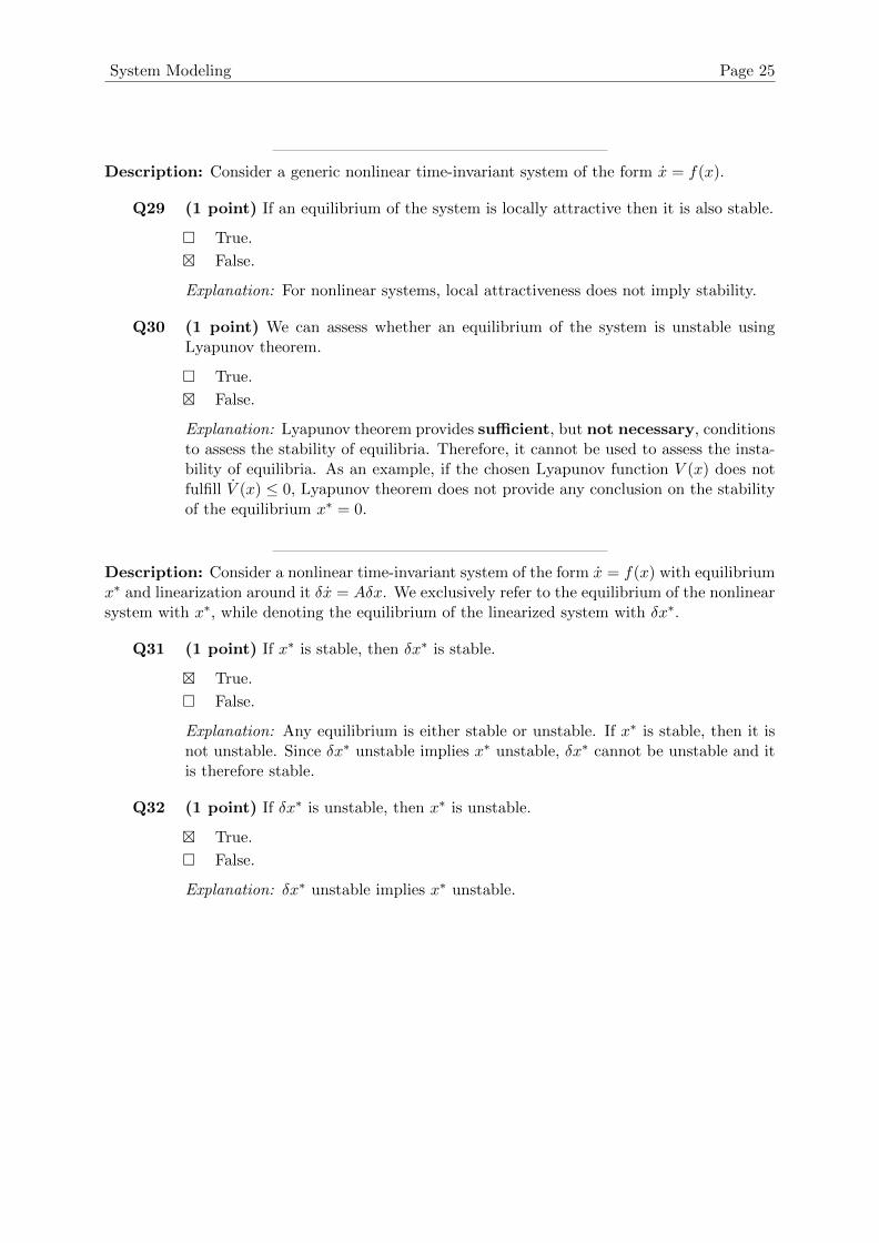
Description: Consider a generic nonlinear time-invariant system of the form x = f(x).
Q29 (1 point) If an equilibrium of the system is locally attractive then it is also stable.
� True.
� False.
Explanation: For nonlinear systems, local attractiveness does not imply stability.
Q30 (1 point) We can assess whether an equilibrium of the system is unstable usingLyapunov theorem.
� True.
� False.
Explanation: Lyapunov theorem provides sufficient, but not necessary, conditionsto assess the stability of equilibria. Therefore, it cannot be used to assess the insta-bility of equilibria. As an example, if the chosen Lyapunov function V (x) does notfulfill V (x) ≤ 0, Lyapunov theorem does not provide any conclusion on the stabilityof the equilibrium x∗ = 0.
Description: Consider a nonlinear time-invariant system of the form x = f(x) with equilibriumx∗ and linearization around it δx = Aδx. We exclusively refer to the equilibrium of the nonlinearsystem with x∗, while denoting the equilibrium of the linearized system with δx∗.
Q31 (1 point) If x∗ is stable, then δx∗ is stable.
� True.
� False.
Explanation: Any equilibrium is either stable or unstable. If x∗ is stable, then it isnot unstable. Since δx∗ unstable implies x∗ unstable, δx∗ cannot be unstable and itis therefore stable.
Q32 (1 point) If δx∗ is unstable, then x∗ is unstable.
� True.
� False.
Explanation: δx∗ unstable implies x∗ unstable.

Page 26 System Modeling
Description: Consider the system x = f(x), with
f(x) =
[x2
−c · x31 − d · x2
],
where c > 0 and d > 0.
Q33 (1 point) Linearize the system around x∗ = 0.
Solution:
A =
[0 10 −d
]Explanation:
A =∂f
∂x
∣∣∣x=x∗=0
=
[0 1
−c · 3 · 02 −d
]=
[0 10 −d
].
Q34 (1 point) What can you conclude regarding the stability of x∗ = 0 usingV (x) = c · x41/4 + x22/2?
� It is unstable.
� It is stable.
� It is locally asymptotically stable.
� It is globally asymptotically stable.
� Nothing.
Explanation: The chosen Lyapunov function V (x) is positive definite (PDF). Sinceits total time derivative is
V (x) =∂V
∂xf(x) = c · x31 · x2 + x2 ·
(− c · x31 − d · x2
)= −d · x22 ≤ 0,
we can conclude that the equilibrium x∗ = 0 is stable. Note that −V (x) is not evenLPDF, since it is 0 for x2 = 0 and any x1.
Q35 (1 point) What can you conclude on the stability of x∗ = 0 from the stability ofδx∗ = 0, assuming
A =
[0 10 −1
]?
� It is unstable.
� It is stable.
� It is locally asymptotically stable.
� It is globally asymptotically stable.
� Nothing.
Explanation: The eigenvalues of A are 0 and −1 (since the matrix is triangular,we can directly read them on the diagonal), which means that δx∗ = 0 is stable.Therefore, we cannot conclude anything for x∗ = 0.
System Modeling Page 27
Description: Consider the linear time-invariant (LTI) system x = Ax with x = [x1, x2]> ∈ R2
and
A =
[0 1−1 −1
].
Given the Lyapunov equation A>P + PA = −Q, you want to compute a Lyapunov functionV (x) = x>Px such that Q = 2I, whereby I ∈ R2×2 is the identity matrix.
Q36 (1 point) What is the total time derivative of the Lyapunov function?
Solution:
V (x) = −2 · x>x = −2 ·(x21 + x22
)Explanation: From the Lyapunov equation we know that, if and only if A isHurwitz (as it is the case),
V (x) = −x>Qx = −2 · x>x = −2 · (x21 + x22).
Description: Consider a linear time-invariant (LTI) system of the form
x =
[−1 0∗ ∗
]x+
[01
]u
y =
[1 00 1
]x,
whereby you forgot the full dynamics of x2.
Q37 (1 point) What can you conclude on the reachability of the system?
� Nothing.
� It is reachable.
� It is not reachable.
Explanation: From inspection, we see that the dynamics of x1 depend only from x1itself. Alternatively, the reachability matrix of the system is
R2 =[B AB
]=
[0 01 ∗
],
which is rank deficient.

Page 28 System Modeling
Q38 (1 point) What can you conclude on the observability of the system?
� Nothing.
� It is observable.
� It is not observable.
Explanation: Since already C has full rank, we can directly conclude that the ob-servability matrix will have full rank and, hence, the system will be observable.Alternatively, the observability matrix can be computed as
O2 =
[CCA
]=
1 00 1−1 0∗ ∗
and has full rank.
Description: Consider a linear time-invariant (LTI) system of the form
x =
[−1
2 00 −2
]x+
[02
]u
y =
[1 00 4
]x.
Q39 (2 points) What is the observability Gramian?
Solution:
WO =
[1 00 4
]Explanation: The observability Gramian WO = W>O can be computed withthe Lyapunov equation as
A>WO +WOA = −C>C ⇐⇒[−1
2 00 −2
] [w1 w2
w2 w3
]+
[w1 w2
w2 w3
] [−1
2 00 −2
]= −
[1 00 4
] [1 00 4
]⇐⇒[
−w1 −52w2
−52w2 −4w3
]=
[−1 00 −16
]⇐⇒
w1 = 1, w2 = 0, w3 = 4 ⇐⇒ WO =
[1 00 4
].

System Modeling Page 29
Description: Consider a linear time-invariant (LTI) system of the form
x = Ax+Bu
y = Cx.
Q40 (1 point) Suppose that WR = WO = diag{1, 100, 10}. Which state variable shouldyou discard when performing a balanced order reduction?
� x1
� x2
� x3
Explanation: When performing a balanced order reduction, we delete the state vari-ables with the smallest diagonal entries in the controllability/reachability Gramian.