solution of electromagnetic and velocity fields forthesai.org/downloads/volume2no1/paper 7-solution...

(IJACSA) International Journal of Advanced Computer Science and Applications,

Vol. 2, No.1, January 2011

42 | P a g e

http://ijacsa.thesai.org/

Solution of Electromagnetic and Velocity Fields for

an Electrohydrodynamic Fluid Dynamical System

Rajveer S Yaduvanshi

AIT, Govt. of Delhi

Delhi, India

[email protected]

Harish Parthasarathy

NSIT, Govt of Delhi

Delhi, India

[email protected]

Abstract— We studied the temporal evolution of the

electromagnetic and velocity fields in an incompressible

conducting fluid by means of computer simulations from the

Navier Stokes and Maxwell’s equations. We then derived the set

of coupled partial differential equations for the stream function

vector field and the electromagnetic field. These equations are

first order difference equations in time and fetch simplicity in

discretization. The spatial partial derivatives get converted into

partial difference equations. The fluid system of equations is thus

approximated by a nonlinear state variable system. This system

makes use of the Kronecker Tensor product. The final system has

taken account of anisotropic permittivity. The conductivity and

magnetic permeability of the fluid are assumed to be

homogeneous and isotropic. Present work in this paper describes

characterization of magneto hydrodynamic anisotropic medium

due to permittivity. Also an efficient and modified novel

numerical solution using Tensor product has been proposed. This

numerical technique seems to be potentially much faster and

provide compatibility in matrices operation. Application of our

characterization technique shall be very useful in tuning of

permittivity in Liquid crystal polymer, Plasma and Dielectric lens

antennas for obtaining wide bandwidth, resonance frequency

reconfigure ability and better beam control.

Keywords- Permittivity tuning, Incompressible fluid, Navier-

Maxwell’s coupled equations, resonance frequency reconfigure

ability.

I. INTRODUCTION

Electro magneto hydrodynamic equation solutions in the field of fluid dynamic have been very recent in many of the applications in the current era [1]. In recent years, there has been a growing interest of research in the interaction between ionic currents in electrolyte solutions and magnetic fields. Electro magneto hydrodynamics (EMHD) is the academic discipline which studies the dynamics of electrically conducting fluids [1-2]. Examples of such fluids include plasmas, liquid metals, and salty water.

Large magnetic field B produces enhanced spectral transfer in the direction perpendicular to field , which changes the polarization. Wave turbulence (WT) theory was developed for deviations from a strong uniform external magnetic field within the incompressible EMHD model. EMHD turbulence can be characterized as counter propagating

wave. According to Maxwell’s equation direction of energy flow of a plane wave is given by E x B [3-5] .

Material medium, in which an EM field exists is characterized by its constitutive parameters σ, µ, ∊ . The medium is said to linear if σ,µ,∊ are independent of E,H or nonlinear otherwise. It is homogeneous if σ,µ,∊ are not function of space variable or inhomogeneous otherwise. Hence σ,µ,∊ are independent of direction or anisotropic otherwise. In isotropic case , are constants and can be extracted from curl term. In an anisotropic medium, properties are different from isotropic. Anisotropy is inherent in fluid. Anisotropic property provide great flexibility for tuning the spatial variations of electromagnetic waves in a desired manner by manipulating their structure features[13-14] . Based on this principle we investigate all components of turbulence applying theoretical approach and validate the same with FDM numerical method. Investigations on electrical properties and physical characteristics of this medium have been a problem for electromagnetic wave transport. As there is a greater need exists for studying interaction of electromagnetic field and anisotropic medium [9-10], when permittivity takes tensor form. The anisotropy can be realized by solution of 3D MHD equations, fluctuations due to uniform applied magnetic field. When strong field is applied, fluid motion and motion of magnetic field lines are closely coupled [15-17]. Thus anisotropic wave becomes Partial Differential Equations, which are difficult to solve analytically. Studies of these non linear effects in our defined problem have been possible, with customized numerical approach using Kronecker Tensor. If we take anisotropy due to permittivity, hence є becomes an matrix, but µ is scalar number. The permittivity tensor =

[

] can be solved for x,y,z directions to have

solution for dielectric constant.

We study the event when there exists an external electric and magnetic field acting on conducting fluid, exhibits anisotropic behavior and its permittivity takes on tensor form. Here we take on inherent characteristics of conducting fluid which has anisotropic permittivity [6-7]. We take this opportunity of anisotropic nature and use for electromagnetic wave propagation, which can be suitable for antenna bandwidth

mailto:[email protected]

http://en.wikipedia.org/wiki/Academic_discipline

http://en.wikipedia.org/wiki/Academic_discipline

http://en.wikipedia.org/wiki/Dynamics_%28mechanics%29

http://en.wikipedia.org/wiki/Electrical_conduction

http://en.wikipedia.org/wiki/Electrical_conduction

http://en.wikipedia.org/wiki/Fluid

http://en.wikipedia.org/wiki/Plasma_%28physics%29

http://en.wikipedia.org/wiki/Brine



43 | P a g e


increment and size reduction applications. This requires tuning of medium permittivity which could be possible by tensor analysis method [8] . For this we shall explore solution of dynamic fluid equations for which there is a need to develop fluid dynamic equations and solve them, for this we shall be using perturbation theory [11-12] to evaluate stream function , magnetic field , Electric field and Current density as function of time by taking x, y, z as Cartesian coordinates. We have used Kronecker Tensor for numerical solution and simulations have been carried out by MATLAB to validate parameters viz , , We have worked for non linear solution of fluid flow taking medium as anisotropic. We have solved for permittivity tensor with conductivity and permeability are kept as constant. Here we used Kronecker Product , discrete values from 0 to N-1 of x, y, z components to generate sparse matrix. This technique provides approximate solution of different dimensional matrices. Hence all nonlinear parameters can be validated with this method. We have worked for solution of B, E,J and with time in x,y,z coordinates.

We have extended the concept cited in reference [1] where solution of 2D MHD have been proposed, it uses conventional method of numerical solution instead of the proposed work. . This paper is organized in five main sections. Section I deals with introduction and survey part. Section II consists of all formulation developed. Sections III have MATLAB simulation results. Section IV conveys the possible applications of our research work. Section V concludes this paper with future implementations.

Abbreviations :

E - Electric intensity (Volts per meter)

H -Magnetic intensity (ampere per meter)

D- Electric flux density (coulomb per square meter)

B - Magnetic flux density (Weber per square meter)

J - Electric current density (ampere per square meter)

Electric charge density (coulomb per cubic meter)

q - Charge electric

Conductivity

- Permeability

– Permittivity

Stream function

v- Velocity of fluid (meter/second)

Mass density

Pressure, η / Kinetic viscosity

F = J X B Lorentz force

II. FORMULATIONS

MHD is an anisotropic medium. The basic equations are

, t + . =

+ + J x

(1)

And the above equation(1) is based on Navier stokes equation

. D = 0

(2)

. B = 0

(3)

x H = J + D, t

(4)

. E = B, t

(5)

B = H

(6)

D =

(7) where are now 3x3 matrices. In term of

components, they are

∑

∑

J = (E + x B) (10)

If is also a 3x3 matrix, then the last equation can be

expressed as

∑

∑

Here is a cyclic unit vector. We can solve V and B

cross product as

= (12)

= (13)

= (14)

∑

Where = = = 1

= = = 1 Others zero from the cyclic unit vector. Initially let J = 0

and =

Then we derive

. E) = 0 (16)

E ( E) = 0 (17)

This equation describes the propagation of EM waves in a

medium having isotropic permeability but anisotropic permittivity. Assume that the density of the medium is a constant i.e. the fluid is incompressible.

Then the mass conservation equation is . = 0 and hence there is a vector field such that, as we know , = x

The curl of the Navier Stokes equation gives

, t + x ( x ) =

+ ( x (JxB) (18)

Where = x = - Since we can assume without loss of generality



44 | P a g e


. = 0

Thus , t + x (( ) x ( x )) =

x (J x B) (19)

Note that

=

∑

∑

∑

Hence

∑

( ∑

)

Here we have worked for presenting a nonlinear solution of fluid flow taking medium as anisotropic due to permittivity and conductivity and permeability are assumed to be fixed.

Now we have to Solve for , , w.r.t. time from the above equations (1-28).The above equations are self explanatory hence does not need more elaborations. Also we can describe

J x B

= ( x B) x B = | |

+ (B. ). B (23)

Hence equation (1) can be written as

, t + x (( ) x ( x )) =

x (( | |

+ (B. ). B) (24)

Let = A( Matrix)

Hence

, t = [ x (( | |

+ (B. ). B) x (( ) x ( x ) ] (25) From Tensor product analysis when; 0 , y, z

N-1 ; we can formulate table for generating block matrix from the coefficients as follows

.

.

.

.

.

.

.

.

.

.

.

.

.

.

.

.

.

.

From finite difference method it can be discretized as given below

Similarly we can complete column of of table 1 to

form this block matrix form coefficients. This can be generated by computer. The computer generated table 2 in triangular form matrix has been named as matrix A , which shall be used to operate with all the elements of the matrices placed at right side in equation (25). This will enable us to solve the problem. Thus we can now estimate approximate value of stream function. Hence we thus gets the value of , t, results are presented in figure 1-10.

Here electric field E can be expressed as

E, t =

-

(E - x B) (26)

Similarly we can evaluate E, t, simulated results are

presented in fig 18.We have to work for getting solution of Matrix [A] to get its inverse we take help of MATLAB.

, ,

.

.

.

.

, , , Also

x =



45 | P a g e


( , , ) (27)

= ―

= ―

= ―

From Finite difference method, we have

(n, k, l, m) =

[ (n, k + 1, l, m) + (n, k - 1, l, m)

― 2 (n, k, l +1, m) + (n, k, l +1, m) + (n, k, l - 1, m)

― 2 (n, k, l, m) + (n, k, l, m+1) +

(n, k, l, m - 1) ― 2 (n, k, l, m)]

(n, k, l, m) =

(n, k + 1, l, m) + (n, k - 1, l, m)

― 6 (n, k, l m) + (n, k, l +1, m) +

(n, k, l - 1, m) + (n, k, l, m+1) + (n, k, l, m - 1)]

(28)

We get this Matrix A from Kronecker Tensor Product

which is generated by computer .

=*

+ , writing this in lexicographical order for solution.

Thus, Matrix A can be expressed as follows:-

(t, x, y, z) =

(t, 0, 0, 0) (t, 0, 0, 0) (t, 0, 0, 0)

(t, 0, 0, 1) (t, 0, 0, 1) (t, 0, 0, 1)

(t, 0, 0, 2) (t, 0, 0, 2) (t, 0, 0, 2)

. . .

. . .

. . .

(t, 0, 0, N-1) (t, 0, 0, N-1) (t, 0, 0, N-1)

(t, 0, 1, 0) (t, 0, 1, 0) (t, 0, 1, 0)

(t, 0, 1, 1) (t, 0, 1, 1) (t, 0, 1, 1)

. . .

. . .

. . .

(t, 0, 1, N-1) (t, 0, 1, N-1) (t, 0, 1, N-1)

. . .

. . .

. . .

(t, N-1, 0, 0) (t, N-1, 0, 0) (t, N-1, 0, 0)

. . .

. . .

. . .

(t, N-1, N-1, N-1) (t, N-1, N-1, N-1)

(t, N-1, N- 1, N-1)

Table 1 Generated from Kronecker Tensor

= *

+ where A Matrix =

Solution of MHD equation

A =

-2 1 0 0 0 0 0 0 0 0 0 0

1 -2 1 0 0 0 0 0 0 0 0 0

0 1 -2 1 0 0 0 0 0 0 0 0

0 0 1 -2 1 0 0 0 0 0 0 0

0 0 0 1 -2 1 0 0 0 0 0 0

0 0 0 0 1 -2 1 0 0 0 0 0

0 0 0 0 0 1 -2 1 0 0 0 0

0 0 0 0 0 0 1 -2 1 0 0 0

0 0 0 0 0 0 0 1 -2 1 0 0

0 0 0 0 0 0 0 0 1 -2 1 0

0 0 0 0 0 0 0 0 0 1 -2 1

0 0 0 0 0 0 0 0 0 0 1 -2

TABLE 1. A – BLOCK MATRIX GENERATED BY COMPUTER

or *

+ = |

| *

+

Hence this will generate 3 X3 order Matrix. For

example tensor product will look like the given below matrix.

*

+ x *

+

= [

( )

( )

]

Here we have taken value of N =10, Which is significantly

small and convenient to run on the computer as large value of N require much amount of memory, more time to compute. Matrix generated has array of elements and with most of the elements are zero. In this way we notice that these non zero elements values get shifted toward one column right side , when moved from first row to second row and second to third row and so on. It forms a triangular matrix; same is shown in table 2. With the help of Kronecker tensor we are able solve PDE equations in matrix form. Results of the solution are discussed in section 3 of this paper.



46 | P a g e


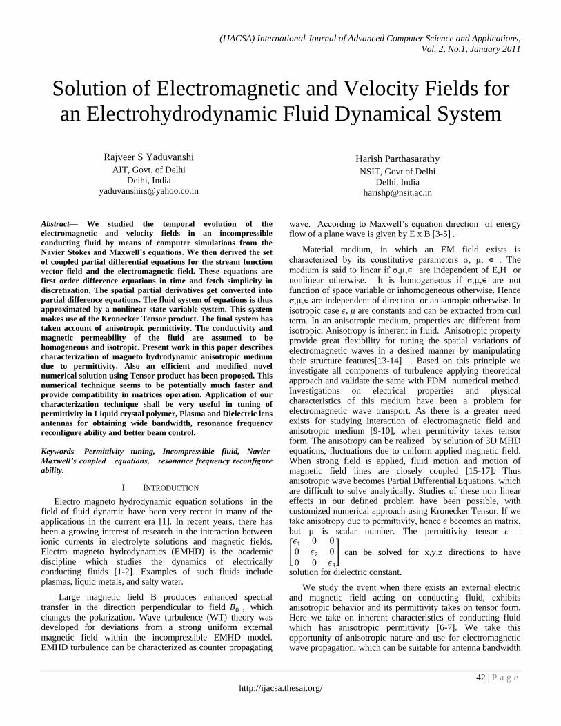
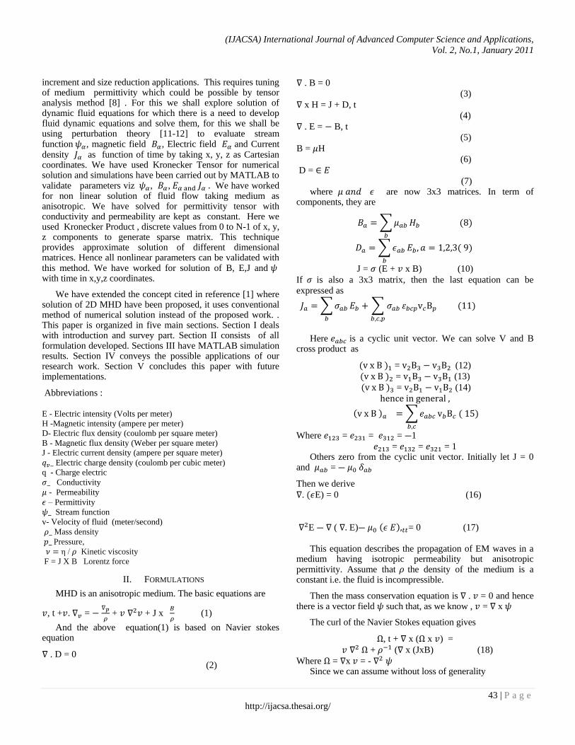
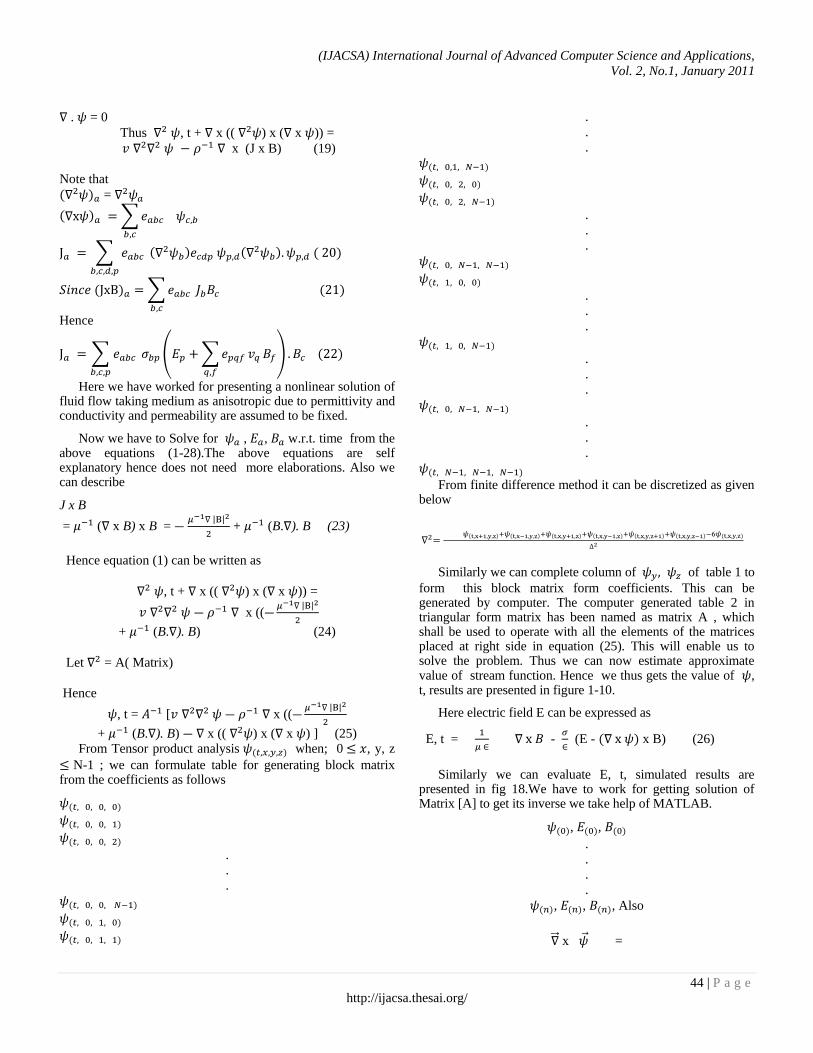
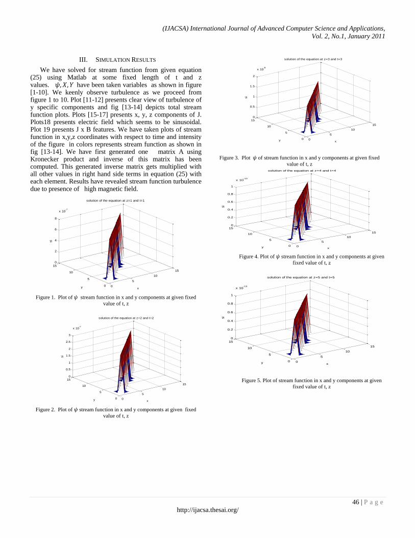
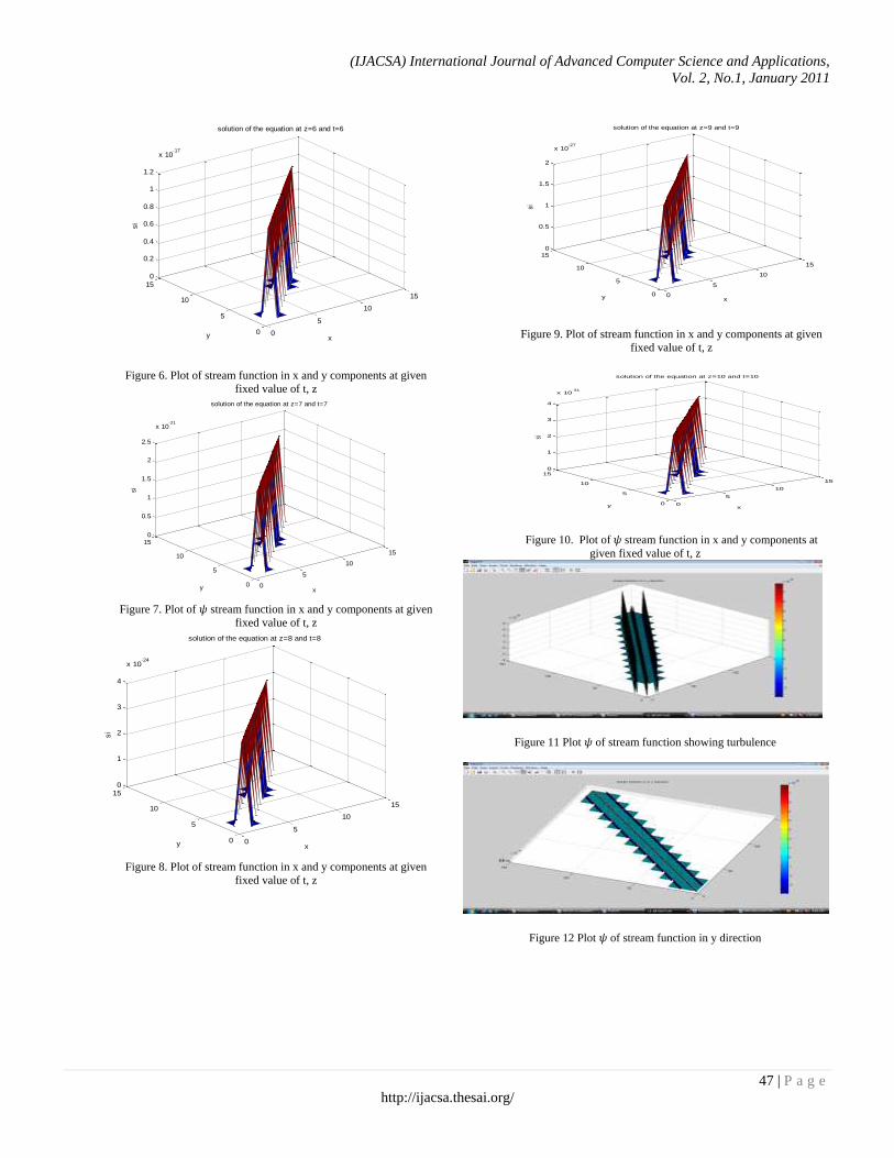
III. SIMULATION RESULTS

We have solved for stream function from given equation (25) using Matlab at some fixed length of t and z values. have been taken variables as shown in figure [1-10]. We keenly observe turbulence as we proceed from figure 1 to 10. Plot [11-12] presents clear view of turbulence of y specific components and fig [13-14] depicts total stream function plots. Plots [15-17] presents x, y, z components of J. Plots18 presents electric field which seems to be sinusoidal. Plot 19 presents J x B features. We have taken plots of stream function in x,y,z coordinates with respect to time and intensity of the figure in colors represents stream function as shown in fig [13-14]. We have first generated one matrix A using Kronecker product and inverse of this matrix has been computed. This generated inverse matrix gets multiplied with all other values in right hand side terms in equation (25) with each element. Results have revealed stream function turbulence due to presence of high magnetic field.

Figure 1. Plot of stream function in x and y components at given fixed

value of t, z


value of t, z


value of t, z

Figure 4. Plot of stream function in x and y components at given

fixed value of t, z


fixed value of t, z

0

5

10

15

0

5

10

150

2

4

6

8

x 10-7

x

solution of the equation at z=1 and t=1

y

si

0

5

10

15

0

5

10

150

0.5

1

1.5

2

2.5

3

x 10-7

x


y

si

0

5

10

15

0

5

10

150

0.5

1

1.5

2

x 10-8

x


y

si0

5

10

15

0

5

10

150

0.2

0.4

0.6

0.8

1

x 10-10

x


y

si

0

5

10

15

0

5

10

150

0.2

0.4

0.6

0.8

1

x 10-13

x


y

si



47 | P a g e



fixed value of t, z


fixed value of t, z


fixed value of t, z


fixed value of t, z

Figure 10. Plot of stream function in x and y components at

given fixed value of t, z

Figure 11 Plot of stream function showing turbulence

Figure 12 Plot of stream function in y direction

0

5

10

15

0

5

10

150

0.2

0.4

0.6

0.8

1

1.2

x 10-17

x


y

si

0

5

10

15

0

5

10

150

0.5

1

1.5

2

2.5

x 10-21

x


y

si

0

5

10

15

0

5

10

150

1

2

3

4

x 10-24

x


y

si

0

5

10

15

0

5

10

150

0.5

1

1.5

2

x 10-27

x


y

si

0

5

10

15

0

5

10

150

1

2

3

4

x 10-31

x


y

si



48 | P a g e


Figure 13. 3D Plot of stream function intensity showing turbulence

Figure 14. 3D plot stream function showing turbulence

Figure15 Plot of J in x axis

Figure16 Plot of J in y axis

Figure 17. Plot of J in z axis

Figure 18. Plot of Electric E field with time

Figure 19 plot of JXB

IV. APPLICATIONS

Permittivity tensor imparts directional dependent properties. Positive permittivity may play significant role for bandwidth and gain in energy propagation. Significant application of this feature can be in designing dielectric lens and LCP antennas. Application of our approach can be an electromagnetically flow control [18] of fluid metal for steel casting with varying magnetic field strength create transition of turbulence due to perturbation. Evaluating field gradient drag effect can predict and control conducting fluid flow. Also in meta material antenna with tuning permittivity may effect in reduction of size of the antenna and these facts are yet to be established as per best of author knowledge. Tele robot, actuator, sensor, EM brakes, Steel casting, Seismic wave, Dielectric lens antenna, Liquid Crystal Polymer antenna, Meta material antenna.

V. CONCLUSION

We have used Kronecker tensor product for numerical

solution to avoid matrices mismatch problem. This numerical approach has not only given us the solution to operate on each other having different order of matrices but also this approach has fetched us the fast computations. An efficient numerical solution technique has been proposed. In this work we have developed 3D MHD equations for turbulence of fluid flow and stream function has been validated in x, y , z direction. Analysis of anisotropic medium for permittivity has been proposed to obtain better transmission parameters. As compared to [1] detailed analyses have been worked with 3D features. Also Numerical techniques developed and used for the present work have been much efficient in computations and time as compared to the previous work cited in reference [1].Turbulence results have been validated with precision control as compared to reference[1].



49 | P a g e


In future works we are busy in working for devising permittivity control and tuning mechanism for anisotropic medium by permittivity tensor analysis, in x, y, z directions to obtain higher dielectric constant which can be the improve efficiency of dielectric lens and liquid crystal antenna. This high dielectric constant or permittivity can also enhance bandwidth and can reduce length of these antennas.

ACKNOWLEDGEMENT AND BIOGRAPHY

My Director Prof Asok De and Director NSIT Prof Raj Senani, who inspired me for this research and enriched me with all necessary resources required for the research. Dr RK Sharma, Associate Professor ECE for fruitful discussions. I am indebted to my wife Sujata, daughter Monica and son Rahul for giving me their time in my research work making home an excellent place for the research.

REFERENCES

[1] Rajveer S Yaduvanshi Harish Parthasarathy, “Design, Development and Simulations of MHD Equations with its proto type implementations”(IJACSA) International Journal of Advanced Computer Science and Applications, Vol. 1, No. 4, October 2010.

[2] EM Lifshitz and LD Landau, “Classical theory of fields , 4th edition Elsevier.

[3] Matthew N.O.Sadiku, “Numerical techniques in Electromagnetic with MATLAB” CRC press, third edition.

[4] EM Lifshitz and LD Landau, “Electrodynamics of continuous media ”Butterworth-Heinemann.

[5] EM Lifshitz and LD Landau,” Theory of Fields”Vol 2 Butterworth-Heinemann.

[6] EM Lifshitz and LD Landau,” Fluid Mechanics”Vol6 ,Butterworth-Heinemann [7]Chorin, A.J., 1986, "Numerical solution of the Navier-Stokes equations", Math. Comp., Vol. 22, pp. 745-762.

[8] Cramer, K.R. &Pai, S., 1973, "Magnetofluid Dynamics For engineers and Applied Physicists", McGraw-Hill BooK.

[9] Feynman, R.P., Leighton, R.B. and Sands, M., 1964, "The Feynman Lectures on Physics", Addison-Wesley, Reading, USA, Chapter 13-1.

[10] Gerbeau, J.F. & Le Bris, C., 1997, "Existence of solution for a density dependant magnetohydrodynamic equation", Advances in Differential Equations, Vol. 2, No. 3, pp. 427-452.

[11] Guermond, J.L. & Shen, J., 2003, "Velocity-correction projection methods for incompressible flows", SIAM J. Numer. Anal. Vol. 41, No. 1, pp. 112-134.

[12] Holman, J.P., 1990, "Heat Transfer" (7th edition), Chapter 12, Special Topics in Heat Transfer, MacGraw-Hill Publishing Company, New York.

[13] PY Picard,”Some spherical solutions of ideal magnetohydrodynamic equation, " Journal of non linear physics vol 14 no4 (2007),578-588. "

[14] Temam, R., 1977, "Navier Stokes Equations ,"Stud. Math. Appl. 2, North-Holland, Amsterdam.

[15] Tillack, M.S. & Morley, N.B., 1998, "MagnetoHydroDynamics", McGraw Hill, Standard Handbook for Electrical Engineers, 14th Edition.

[16] Wait, R. (1979). The numerical solution of algebraic equations. A Wiley-interscience publication.

[17] Fermigier, M. (1999). Hydrodynamique physique. Problèmes résolus avec rappels de cours, collectionsciences sup. physique, edition Dunod.

[18] Bahadir, A.R. and T. Abbasov (2005). A numerical investigation of the liquid flow velocity over an infinity plate which is taking place in a magnetic field. International journal of applied electromagnetic and mechanics 21, 1-10.

AUTHORS PROFILE

Author: Rajveer S Yaduvanshi, Asst Professor has 21 years of teaching and research work. He is fellow member of IETE. He is author of two international journal paper and five international /national conference papers. He has successfully implemented fighter aircraft arresting barrier projects at select flying stations of Indian Air Force. He has worked on Indigenization projects of 3D radars at DGAQA, Min of defense and visited France for 3D radar modernization program as Senior Scientific Officer. Currently he is working on MHD Antenna prototype implementations. At present, he is teaching in ECE Deptt. of AIT , Govt of Delhi-110031.

Co-Author : Prof Harish Parthasarathy is an eminent academician and great researcher . He is professor and dean at NSIT , Govt. College of Engineering at Dwarka, Delhi. He has extra ordinary research instinct and a great book writer in the field of DSP. He has published more than ten books and have produces more than seven PhDs in ECE Deptt of NSIT,Delhi.

solution of electromagnetic and velocity fields forthesai.org/downloads/volume2no1/paper 7-solution...

Documents