solution of an inverse heat conduction problem in a bi-layered spherical tissue
TRANSCRIPT
This article was downloaded by: [Michigan State University]On: 05 October 2013, At: 05:07Publisher: Taylor & FrancisInforma Ltd Registered in England and Wales Registered Number: 1072954 Registeredoffice: Mortimer House, 37-41 Mortimer Street, London W1T 3JH, UK
Numerical Heat Transfer, Part A:Applications: An International Journal ofComputation and MethodologyPublication details, including instructions for authors andsubscription information:http://www.tandfonline.com/loi/unht20
Solution of an Inverse Heat ConductionProblem in a Bi-Layered Spherical TissueKuo-Chi Liu a & Chin-Tse Lin ba Department of Mechanical Engineering, Far East University, Tainan,Taiwan, Republic of Chinab Department of Computer Application Engineering, Far EastUniversity, Tainan, Taiwan, Republic of ChinaPublished online: 19 Nov 2010.
To cite this article: Kuo-Chi Liu & Chin-Tse Lin (2010) Solution of an Inverse Heat Conduction Problemin a Bi-Layered Spherical Tissue, Numerical Heat Transfer, Part A: Applications: An InternationalJournal of Computation and Methodology, 58:10, 802-818, DOI: 10.1080/10407782.2010.523329
To link to this article: http://dx.doi.org/10.1080/10407782.2010.523329
PLEASE SCROLL DOWN FOR ARTICLE
Taylor & Francis makes every effort to ensure the accuracy of all the information (the“Content”) contained in the publications on our platform. However, Taylor & Francis,our agents, and our licensors make no representations or warranties whatsoever as tothe accuracy, completeness, or suitability for any purpose of the Content. Any opinionsand views expressed in this publication are the opinions and views of the authors,and are not the views of or endorsed by Taylor & Francis. The accuracy of the Contentshould not be relied upon and should be independently verified with primary sourcesof information. Taylor and Francis shall not be liable for any losses, actions, claims,proceedings, demands, costs, expenses, damages, and other liabilities whatsoever orhowsoever caused arising directly or indirectly in connection with, in relation to or arisingout of the use of the Content.
This article may be used for research, teaching, and private study purposes. Anysubstantial or systematic reproduction, redistribution, reselling, loan, sub-licensing,systematic supply, or distribution in any form to anyone is expressly forbidden. Terms &Conditions of access and use can be found at http://www.tandfonline.com/page/terms-and-conditions
SOLUTION OF AN INVERSE HEAT CONDUCTIONPROBLEM IN A BI-LAYERED SPHERICAL TISSUE
Kuo-Chi Liu1 and Chin-Tse Lin21Department of Mechanical Engineering, Far East University, Tainan,Taiwan, Republic of China2Department of Computer Application Engineering, Far East University,Tainan, Taiwan, Republic of China
This work attempts to estimate the phase lag times of a tissue based on the dual-phase-lag
model from the experimental data. The inverse dual-phase-lag bioheat transfer problem in
the bilayered spherical tissue is studied. The difference between two layers in the thermo-
physical parameters, geometry effects, and measurement errors of the input data make it
hard to be solved. To solve the present problem, a hybrid scheme based on the Laplace
transform, change of variables, and the least-squares scheme is proposed. In order to evi-
dence the validity and accuracy of the estimated results, the comparison of the history of
temperature increase between the calculated results and the experimental data is made
for various measurement locations. The effect of measurement location on the estimated
results is also investigated.
INTRODUCTION
The use of heat to necrotize undesirable tissue for therapeutic purposes is notan innovative idea. It has been in many applications, such as cauterizing a wound,treating inflammation, and eliminating port wine stains. These days, the use ofhyperthermia has been developed as an important technique to destroy malignanttumors. In hyperthermia, the targeted tissue must be elevated to temperatures inthe range 42�C–46�C for a specified period of time. An ideal hyperthermia treatmentshould selectively destroy the target region without damaging the surroundinghealthy tissue. However, it is not easy to accurately determine the temperature fieldover the entire treatment region during clinical hyperthermia treatments, because thepain tolerance of patients makes the number of invasive temperature probes limited[1]. In order to further improve the thermal treatment methods, many researchershave aimed at hyperthermia treatments. The bioheat models are essential duringdevelopment of equipment, for pre-planning purposes, for online monitoring and
Received 10 February 2010; accepted 7 August 2010.
Support for this work by the National Science Counsel under grant no. NSC 97-2212-E-269-023 is
gratefully acknowledged.
Address correspondence to Kuo-Chi Liu, Department of Mechanical Engineering, Far East
University, 49 Chung Hua Rd., Hsin-Shih, Tainan 744, Taiwan, Republic of China. E-mail: kcliu@
cc.feu.edu.tw
Numerical Heat Transfer, Part A, 58: 802–818, 2010
Copyright # Taylor & Francis Group, LLC
ISSN: 1040-7782 print=1521-0634 online
DOI: 10.1080/10407782.2010.523329
802
Dow
nloa
ded
by [
Mic
higa
n St
ate
Uni
vers
ity]
at 0
5:07
05
Oct
ober
201
3
decision support, as well as for evaluation of the extent of thermal damage [2].Therefore, one of the ways current research seeks improvement is to develop a heattransfer model for the analysis and modeling of the underlying thermal mechanismsin the treated region.
Most analyses of temperature predictions for biological bodies are based on thewell-known Pennes’ bioheat equation. The Pennes’ bioheat equation was derivedwith the classical Fourier’s law that depicts an infinite velocity of thermal propa-gation. However, the contents of the literature [3–7] indicated that thermal behaviorin biological tissues requires a relaxation time to accumulate enough energy to trans-fer to the nearest element. The relevant researchers [8–11], thus employed the ther-mal wave model to remedy this physically unreasonable deficiency. The thermalwave model cannot capture the microstructural interaction effects [12], and intro-duce some unusual behaviors and physical solutions [13–15]. The thermal wavemodel becomes open to debate for its validity.
In order to explore another possibility, Antaki [16] used the dual-phase-lag(DPL) heat conduction model to interpret the thermal behavior in processed meats.The DPL model describes a macroscopic temperature with the microstructural effectby introducing the phase lag times of heat flux and temperature gradient. Followingin Antaki’s steps, there are a few papers that study the bioheat transfer problemswith the DPL model. Liu and Chen [17] studied temperature rise behavior in atwo-layer concentric spherical region during magnetic tumor hyperthermia treatment
NOMENCLATURE
A estimated parameter
c specific heat of tissue, J=kg �Kcb specific heat of blood, J=kg �Kdn correction of An
em deviation between hcalm and hmeam
f parameter defined in Eq. (20)
H new dependent variable,
H¼ r(T�T0)eHH Laplace transform of H
k thermal conductivity, W=m �KK parameter defined in Eq. (21)
‘ distance between two neighboring
nodes, m
M total number of nodes
N total number of estimated parameters
P power density, W=m3
qm metabolic heat generation, W=m3
qr spatial heating source, W=m3
r space coordinate, m
R radius of tumor, m
s Laplace transform parameter
t time, s
T temperature of tissue, K
Tb arterial temperature, K
T0 initial temperature of tissue, K
wb perfusion rate of blood, m3=s=m3
xmn parameter defined in Eq. (34)
dmn Kronecker delta
h temperature increase defined in
Eq. (27)
e standard deviation of the
measurements
k parameter defined in Eq. (19)
q density, kg=m3
w volume fraction of magnetic particles
sq phase lag of the heat flux, s
sT phase lag of the temperature gradient,
s
Superscripts
cal calculated value
mea measured data
Subscripts
g magnetic particle
i node number
j number of sub-space domain
k number of layer
m number of time node
n number of estimated parameter
t tumor tissue
INVERSE PROBLEM IN SPHERICAL TISSUE 803
Dow
nloa
ded
by [
Mic
higa
n St
ate
Uni
vers
ity]
at 0
5:07
05
Oct
ober
201
3
with the DPL model. Zhou et al. [18] recently proposed a two-dimensionalaxisymmetric DPL model to describe heat transfer in living biological tissues withnonhomogenous inner structures. Zhang [19] derived the general dual phase bio-heat equations from the nonequilibrium model for living biological tissues. How-ever, there is limited experimental evidence for showing the physical meanings ofthe DPL mode in the bioheat transfer.
This work attempts to estimate the phase lag times based on the DPLmodel from the experimental data given by Andra et al. [20]. The inverse problemis an ill-posed problem. Various methods [21–25] were developed for the inverseheat conduction problems. However, it is well-known that there are mathematicaldifficulties in dealing with the non-Fourier heat transfer problem, not to mentionthe inverse problem is an ill-posed problem. The literature about the estimationof the relaxation times in tissues are not numerous. Aside from references [4–7,16], the literature [26–30] mainly estimated the boundary conditions with the ana-lytical solution in conjunction with measurement errors. Due to the differencebetween two layers in the thermophysical parameters, geometry effects, andmeasurement errors of the input data, the present problem introduces complexityand causes more mathematical difficulties. To solve the present problem, a hybridnumerical scheme based on the Laplace transform, change of variables, and theleast-squares scheme is proposed. In order to evidence the validity and accuracyof the estimated results, the comparisons of the temperature increase historybetween the results calculated with the estimates and the experimental data aremade for various measurement locations. The solution of inverse problem willdepend on location [31]. Therefore, the investigation of the effect of locationon the estimated results is involved.
MATHEMATICS MODEL
To accommodate the microstructural effect, the DPL model suggested by Tzou[32] is applied. The linear version of the DPL model is expressed as
sqqqqt
þ q ¼ �kqTqr
� ksTq2Tqtqr
ð1Þ
where T is the temperature and q is the heat flux. sq means the phase lag of the heatflux and sT means the phase lag of the temperature gradient. In bioheat transfer,Antaki [16] interpreted sq as a delay time for contact resistance between tissue par-ticles. On the other hand, sT was interpreted as a measure of the conduction thatoccurs within tissues particles. The values of sq and sT may be different in tumorand normal tissue as well as the other physiological parameters. The heat flux pre-cedes the temperature gradient for sq< sT. The temperature gradient precedes theheat flux for sq> sT. The DPL model combines the wave features of hyperbolic con-duction with a diffusion-like feature of the evidence not captured by the hyperboliccase. As sT¼ 0, the DPL model reduces to the thermal wave model of heat transfer.By further letting sq¼ 0, it becomes the classical Fourier law.
In magnetic tumor hyperthermia, fine magnetic particles are localized at thetumor tissue. The literature [20, 33, 34] regarded the small tumor as a solid
804 K.-C. LIU AND C.-T. LIN
Dow
nloa
ded
by [
Mic
higa
n St
ate
Uni
vers
ity]
at 0
5:07
05
Oct
ober
201
3
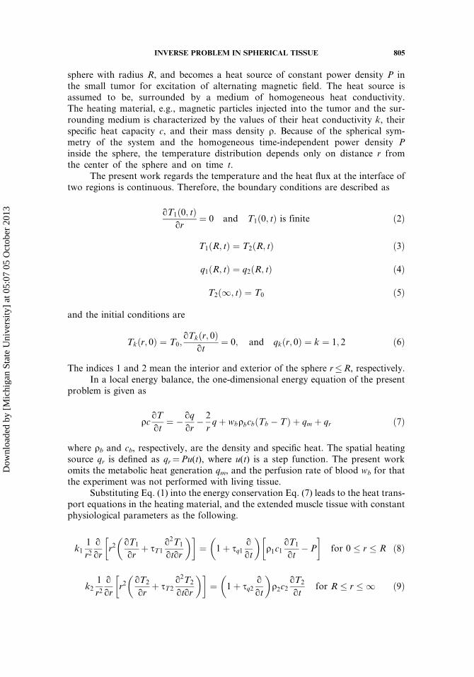
sphere with radius R, and becomes a heat source of constant power density P inthe small tumor for excitation of alternating magnetic field. The heat source isassumed to be, surrounded by a medium of homogeneous heat conductivity.The heating material, e.g., magnetic particles injected into the tumor and the sur-rounding medium is characterized by the values of their heat conductivity k, theirspecific heat capacity c, and their mass density q. Because of the spherical sym-metry of the system and the homogeneous time-independent power density Pinside the sphere, the temperature distribution depends only on distance r fromthe center of the sphere and on time t.
The present work regards the temperature and the heat flux at the interface oftwo regions is continuous. Therefore, the boundary conditions are described as
qT1ð0; tÞqr
¼ 0 and T1ð0; tÞ is finite ð2Þ
T1ðR; tÞ ¼ T2ðR; tÞ ð3Þ
q1ðR; tÞ ¼ q2ðR; tÞ ð4Þ
T2ð1; tÞ ¼ T0 ð5Þ
and the initial conditions are
Tkðr; 0Þ ¼ T0;qTkðr; 0Þ
qt¼ 0; and qkðr; 0Þ ¼ k ¼ 1; 2 ð6Þ
The indices 1 and 2 mean the interior and exterior of the sphere r�R, respectively.In a local energy balance, the one-dimensional energy equation of the present
problem is given as
qcqTqt
¼ � qqqr
� 2
rqþ wbqbcbðTb � TÞ þ qm þ qr ð7Þ
where qb and cb, respectively, are the density and specific heat. The spatial heatingsource qr is defined as qr¼Pu(t), where u(t) is a step function. The present workomits the metabolic heat generation qm, and the perfusion rate of blood wb for thatthe experiment was not performed with living tissue.
Substituting Eq. (1) into the energy conservation Eq. (7) leads to the heat trans-port equations in the heating material, and the extended muscle tissue with constantphysiological parameters as the following.
k11
r2qqr
�r2�qT1
qrþ sT1
q2T1
qtqr
��¼
�1þ sq1
qqt
��q1c1
qT1
qt� P
�for 0 � r � R ð8Þ
k21
r2qqr
�r2�qT2
qrþ sT2
q2T2
qtqr
��¼
�1þ sq2
qqt
�q2c2
qT2
qtfor R � r � 1 ð9Þ
INVERSE PROBLEM IN SPHERICAL TISSUE 805
Dow
nloa
ded
by [
Mic
higa
n St
ate
Uni
vers
ity]
at 0
5:07
05
Oct
ober
201
3
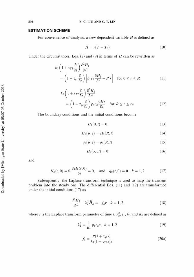
ESTIMATION SCHEME
For convenience of analysis, a new dependent variable H is defined as
H ¼ rðT � T0Þ ð10Þ
Under the circumstances, Eqs. (8) and (9) in terms of H can be rewritten as
k1
�1þ sT1
qqt
�q2H1
qr2
¼�1þ sq1
qqt
��q1c1
qH1
qt� P r
�for 0 � r � R ð11Þ
k2
�1þ sT2
qqt
�q2H2
qr2
¼�1þ sq2
qqt
�q2c2
qH2
qtfor R � r � 1 ð12Þ
The boundary conditions and the initial conditions become
H1ð0; tÞ ¼ 0 ð13Þ
H1ðR; tÞ ¼ H2ðR; tÞ ð14Þ
q1ðR; tÞ ¼ q2ðR; tÞ ð15Þ
H2ð1; tÞ ¼ 0 ð16Þ
and
Hkðr; 0Þ ¼ 0;qHkðr; 0Þ
qt¼ 0; and qkðr; 0Þ ¼ 0 k ¼ 1; 2 ð17Þ
Subsequently, the Laplace transform technique is used to map the transientproblem into the steady one. The differential Eqs. (11) and (12) are transformedunder the initial conditions (17) as
d2 eHHk
dr2� k2k eHHk ¼ �fkr k ¼ 1; 2 ð18Þ
where s is the Laplace transform parameter of time t. k2k, f1, f2, and Kk are defined as
k2k ¼1
Kkqkcks k ¼ 1; 2 ð19Þ
f1 ¼Pð1þ sq1sÞk1ð1þ sT1sÞs
ð20aÞ
806 K.-C. LIU AND C.-T. LIN
Dow
nloa
ded
by [
Mic
higa
n St
ate
Uni
vers
ity]
at 0
5:07
05
Oct
ober
201
3
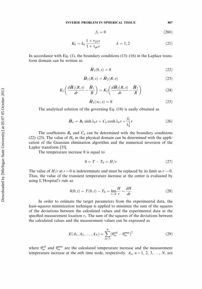
f2 ¼ 0 ð20bÞ
Kk ¼ kk1þ sTks1þ sqks
k ¼ 1; 2 ð21Þ
In accordance with Eq. (1), the boundary conditions (13)–(16) in the Laplace trans-form domain can be written as
eHH1ð0; sÞ ¼ 0 ð22Þ
eHH1ðR; sÞ ¼ eHH2ðR; sÞ ð23Þ
K1
�d eHH1ðR; sÞ
dr�
eHH1
R
�¼ K2
�d eHH2ðR; sÞ
dr�
eHH2
R
�ð24Þ
eHH2ð1; sÞ ¼ 0 ð25Þ
The analytical solution of the governing Eq. (18) is easily obtained as
eHHk ¼ Bk sinh kkrþ Ck cosh kkrþfk
k2kr ð26Þ
The coefficients Bk and Ck can be determined with the boundary conditions(22)–(25). The value of Hk in the physical domain can be determined with the appli-cation of the Gaussian elimination algorithm and the numerical inversion of theLaplce transform [35].
The temperature increase h is equal to
h ¼ T � T0 ¼ H=r ð27Þ
The value of H=r at r¼ 0 is indeterminate and must be replaced by its limit as r! 0.Thus, the value of the transient temperature increase at the center is evaluated byusing L’Hospital’s rule as
hð0; tÞ ¼ Tð0; tÞ � T0 ¼ limr!0
H
r¼ dH
drð28Þ
In order to estimate the target parameters from the experimental data, theleast-squares minimization technique is applied to minimize the sum of the squaresof the deviations between the calculated values and the experimental data at thespecified measurement location ri. The sum of the squares of the deviations betweenthe calculated values and the measurement values can be expressed as
EðA1;A2; . . . ;ANÞ ¼XNm¼1
ðhcalm � hmeam Þ2 ð29Þ
where hcalm and hmeam are the calculated temperature increase and the measurement
temperature increase at the mth time node, respectively. An, n¼ 1, 2, 3, . . . , N, are
INVERSE PROBLEM IN SPHERICAL TISSUE 807
Dow
nloa
ded
by [
Mic
higa
n St
ate
Uni
vers
ity]
at 0
5:07
05
Oct
ober
201
3
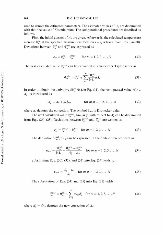
used to denote the estimated parameters. The estimated values of An are determinedwith that the value of E is minimum. The computational procedures are described asfollows.
First, the initial guesses of An are given. Afterwards, the calculated temperature
increase hcalm at the specified measurement location r¼ ri is taken from Eqs. (26–28).
Deviations between hcalm and hmeam are expressed as
em ¼ hcalm � hmeam for m ¼ 1; 2; 3; . . . ;N ð30Þ
The next calculated value hcal;�m can be expanded in a first-order Taylor series as
hcal;�m ¼ hcalm þXNn¼1
qhcalm
qAndAn ð31Þ
In order to obtain the derivative qhcalm =qAnin Eq. (31), the next guessed value of An,A�
n, is introduced as
A�n ¼ An þ dndmn for m; n ¼ 1; 2; 3; . . . ;N ð32Þ
where dn denotes the correction. The symbol dmn is Kronecker delta.
The next calculated value hcal;�m , similarly, with respect to A�n can be determined
from Eqs. (26)–(28). Deviations between hcal;�m and hmeam are written as
e�m ¼ hcal;�m � hmeam for m ¼ 1; 2; 3; . . . ;N ð33Þ
The derivative qhcalm =qAn can be expressed in the finite-difference form as
xmn ¼qhcalm
qAn¼ hcal;�m � hmea
m
A�n � An
for m; n ¼ 1; 2; 3; . . . ;N ð34Þ
Substituting Eqs. (30), (32), and (33) into Eq. (34) leads to
xmn ¼e�m � em
dnfor m; n ¼ 1; 2; 3; . . . ;N ð35Þ
The substitution of Eqs. (34) and (35) into Eq. (31) yields
hcal;�m ¼ hcalm þXNn¼1
xmnd�n for m ¼ 1; 2; 3; . . . ;N ð36Þ
where d�n ¼ dAn denotes the new correction of An.
808 K.-C. LIU AND C.-T. LIN
Dow
nloa
ded
by [
Mic
higa
n St
ate
Uni
vers
ity]
at 0
5:07
05
Oct
ober
201
3
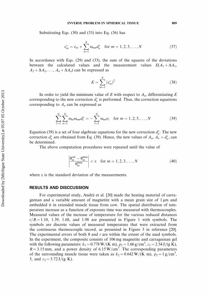
Substituting Eqs. (30) and (33) into Eq. (36) has
e�m ¼ em þXNn¼1
xmnd�n for m ¼ 1; 2; 3; . . . ;N ð37Þ
In accordance with Eqs. (29) and (33), the sum of the squares of the deviationsbetween the calculated values and the measurement values E(A1þDA1,A2þDA2, . . . , AnþDAn) can be expressed as
E ¼XNm¼1
ðe�mÞ2 ð38Þ
In order to yield the minimum value of E with respect to An, differentiating Ecorresponding to the new correction d�
n is performed. Thus, the correction equationscorresponding to An can be expressed as
XNl¼1
XNn¼1
xnlxmnd�l ¼ �
XNl¼1
xmlel for m ¼ 1; 2; 3; . . . ;N ð39Þ
Equation (39) is a set of four algebraic equations for the new correction d�n . The new
correction d�n are obtained from Eq. (39). Hence, the new values of An, An þ d�
n , canbe determined.
The above computation procedures were repeated until the value of
hcalm � hmeam
hmeam
���������� < e for m ¼ 1; 2; 3; . . . ;N ð40Þ
where e is the standard deviation of the measurements.
RESULTS AND DISCCUSSION
For experimental study, Andra et al. [20] made the heating material of carra-geenan and a variable amount of magnetite with a mean grain size of 1 mm andembedded it in extended muscle tissue from cow. The spatial distribution of tem-perature increase as a function of exposure time was measured with thermocouples.Measured values of the increase of temperature for the various reduced distancesr=R¼ 1.10, 1.39, 1.68, and 1.98 are presented in Figure 1 with symbols. Thesymbols are discrete values of measured temperature that were extracted fromthe continuous thermocouple record, as presented in Figure 3 in reference [20].The experimental errors of both h and t are within the extent of the used symbols.In the experiment, the composite consists of 106mg magnetite and carrageenan gelwith the following parameters: k1¼ 0.778W=(K m), q1¼ 1.66 g=cm3, c1¼ 2.54 J=(g K),R¼ 3.15mm, and a power density of 6.15W=cm3. The corresponding parametersof the surrounding muscle tissue were taken as k2¼ 0.642W=(K m), q2¼ 1 g=cm3,3, and c2¼ 3.72 J=(g K).
INVERSE PROBLEM IN SPHERICAL TISSUE 809
Dow
nloa
ded
by [
Mic
higa
n St
ate
Uni
vers
ity]
at 0
5:07
05
Oct
ober
201
3
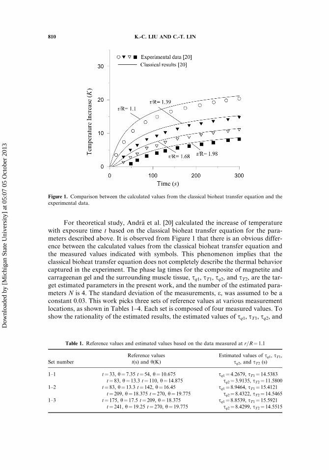
For theoretical study, Andra et al. [20] calculated the increase of temperaturewith exposure time t based on the classical bioheat transfer equation for the para-meters described above. It is observed from Figure 1 that there is an obvious differ-ence between the calculated values from the classical bioheat transfer equation andthe measured values indicated with symbols. This phenomenon implies that theclassical bioheat transfer equation does not completely describe the thermal behaviorcaptured in the experiment. The phase lag times for the composite of magnetite andcarrageenan gel and the surrounding muscle tissue, sq1, sT1, sq2, and sT2, are the tar-get estimated parameters in the present work, and the number of the estimated para-meters N is 4. The standard deviation of the measurements, e, was assumed to be aconstant 0.03. This work picks three sets of reference values at various measurementlocations, as shown in Tables 1–4. Each set is composed of four measured values. Toshow the rationality of the estimated results, the estimated values of sq1, sT1, sq2, and
Table 1. Reference values and estimated values based on the data measured at r=R¼ 1.1
Set number
Reference values
t(s) and h(K)
Estimated values of sq1, sT1,sq2, and sT2 (s)
1–1 t¼ 33, h¼ 7.35 t¼ 54, h¼ 10.675
t¼ 83, h¼ 13.3 t¼ 110, h¼ 14.875
sq1¼ 4.2679, sT1¼ 14.5383
sq2¼ 3.9135, sT2¼ 11.5800
1–2 t¼ 83, h¼ 13.3 t¼ 142, h¼ 16.45
t¼ 209, h¼ 18.375 t¼ 270, h¼ 19.775
sq1¼ 8.9464, sT1¼ 15.4121
sq2¼ 8.4322, sT2¼ 14.5465
1–3 t¼ 175, h¼ 17.5 t¼ 209, h¼ 18.375
t¼ 241, h¼ 19.25 t¼ 270, h¼ 19.775
sq1¼ 8.8539, sT1¼ 15.5921
sq2¼ 8.4299, sT2¼ 14.5515
Figure 1. Comparison between the calculated values from the classical bioheat transfer equation and the
experimental data.
810 K.-C. LIU AND C.-T. LIN
Dow
nloa
ded
by [
Mic
higa
n St
ate
Uni
vers
ity]
at 0
5:07
05
Oct
ober
201
3
sT2 would bring into Eqs. (26)–(28) to calculate the increase of temperature withexposure time t at various reduced distances. Figures 2–5 show the comparison ofthe calculated results with the experimental data.
Table 1 shows the three sets of reference values chosen from the data measuredat r=R¼ 1.10 and the estimated results. It is found that the estimated values of sq1,sT1, sq2, and sT2 for set 1–2 almost agree with those for set 1–3, but are obviouslydifferent with those for set 1–1. However, the calculated results of the increase oftemperature with exposure time t for these three sets are very similar and approachthe experimental data at various reduced distances, as shown in Figure 2. The timenodes are 33 s, 54 s, 83 s, and 110 s for the reference values of set 1–1. The history oftemperature increase with sq1¼ 4.2679s, sT1¼ 14.5383 s, sq2¼ 3.9135 s, andsT2¼ 11.5800 s coincides with the experimental data at the reduced distancer=R¼ 1.10 during 0 s� t� 150 s, but does not coincide at the reduced distancesr=R¼ 1.39, 1.68, and 1.98. After t¼ 150 s, it gradually splits from the experimental
Table 3. Reference values and estimated values based on the data measured at r=R¼ 1.68
Set number
Reference values
t(s) and h(K)
Estimated values
of sq1, sT1, sq2, and sT2, (s)
3–1 t¼ 32, h¼ 1.225 t¼ 48, h¼ 2.625
t¼ 64, h¼ 3.675 t¼ 109, h¼ 6.125
sq1¼ 12.9945, sT1¼ 5.3008
sq2¼ 12.2865, sT2¼ 18.9981
3–2 t¼ 109, h¼ 6.125 t¼ 129, h¼ 7.175
t¼ 157, h¼ 8.225 t¼ 212, h¼ 9.45
sq1¼ 6.6475, sT1¼ 20.6194
sq2¼ 6.3299, sT2¼ 17.0494
3–3 t¼ 129, h¼ 7.175 t¼ 157, h¼ 11.2
t¼ 212, h¼ 12.775 t¼ 274, h¼ 14
sq1¼ 7.5586, sT1¼ 21.9667
sq2¼ 7.401, sT2¼ 17.8216
Table 4. Reference values and estimated values based on the data measured at r=R¼ 1.98
Set number
Reference values
t(s) and h(K)
Estimated values of sq1, sT1,sq2, and sT2 (s)
4–1 t¼ 49, h¼ 0.875 t¼ 64, h¼ 1.925
t¼ 86, h¼ 3.15 t¼ 109, h¼ 4.025
——–
4–2 t¼ 109, h¼ 4.025 t¼ 157, h¼ 5.6
t¼ 212, h¼ 6.65 t¼ 274, h¼ 7.875
sq1¼ 8.1768, sT1¼ 22.5628
sq2¼ 7.7672, sT2¼ 21.3071
4–3 t¼ 129, h¼ 4.725 t¼ 157, h¼ 5.6
t¼ 212, h¼ 6.65 t¼ 274, h¼ 7.875
sq1¼ 6.1462, sT1¼ 28.7482
sq2¼ 5.7370, sT2¼ 22.5038
Table 2. Reference values and estimated values based on the data measured at r=R¼ 1.39
Set number
Reference values
t(s) and h(K)
Estimated values of
sq1, sT1, sq2, and sT2 (s)
2–1 t¼ 32, h¼ 2.8 t¼ 48, h¼ 4.9
t¼ 64, h¼ 6.3 t¼ 86, h¼ 8.05
——–
2–2 t¼ 109, h¼ 9.1 t¼ 157, h¼ 11.2
t¼ 212, h¼ 12.775 t¼ 274, h¼ 14
sq1¼ 7.6140, sT1¼ 20.1088
sq2¼ 7.3629, sT2¼ 18.7825
2–3 t¼ 157, h¼ 11.2 t¼ 184, h¼ 12.25
t¼ 240, h¼ 13.475 t¼ 274, h¼ 14
sq1¼ 8.3776, sT1¼ 18.6416
sq2¼ 8.0022, sT2¼ 17.7723
INVERSE PROBLEM IN SPHERICAL TISSUE 811
Dow
nloa
ded
by [
Mic
higa
n St
ate
Uni
vers
ity]
at 0
5:07
05
Oct
ober
201
3

Figure 2. History of temperature increase with the estimated values of sq1, sT1, sq2, and sT2 based on the
experimental data at r=R¼ 1.1.
Figure 3. History of temperature increase with the estimated values of sq1, sT1, sq2, and sT2 based on the
experimental data at r=R¼ 1.39.
812 K.-C. LIU AND C.-T. LIN
Dow
nloa
ded
by [
Mic
higa
n St
ate
Uni
vers
ity]
at 0
5:07
05
Oct
ober
201
3
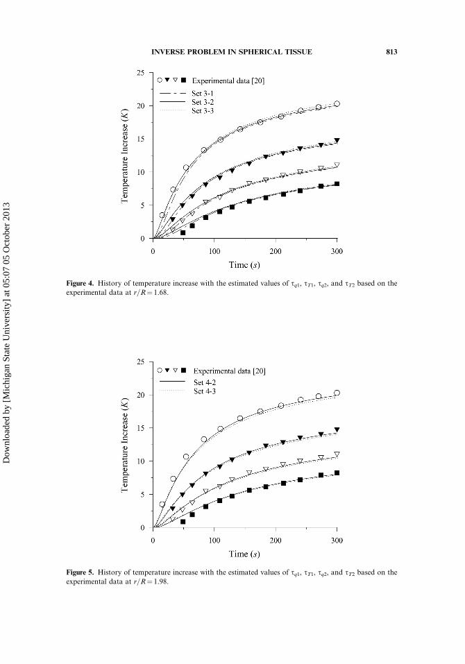
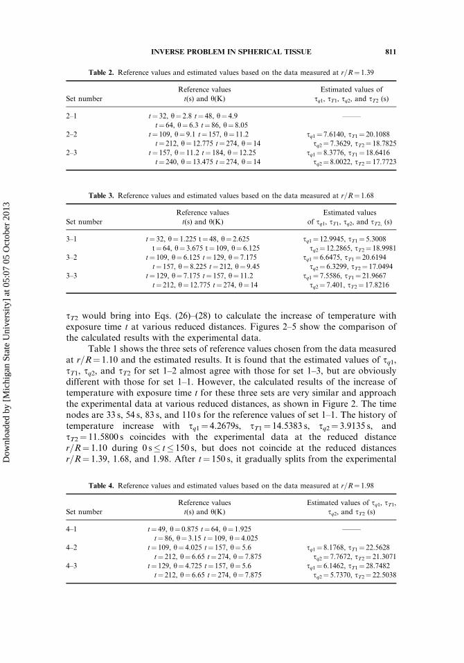
Figure 4. History of temperature increase with the estimated values of sq1, sT1, sq2, and sT2 based on the
experimental data at r=R¼ 1.68.
Figure 5. History of temperature increase with the estimated values of sq1, sT1, sq2, and sT2 based on the
experimental data at r=R¼ 1.98.
INVERSE PROBLEM IN SPHERICAL TISSUE 813
Dow
nloa
ded
by [
Mic
higa
n St
ate
Uni
vers
ity]
at 0
5:07
05
Oct
ober
201
3
data. These phenomena do not exist for set 1–2 and set 1–3. In the meantime, thecurves of the history of temperature increase gradually approach consistent withthe reduced distance increasing for sets 1–1, 1–2, and 1–3.
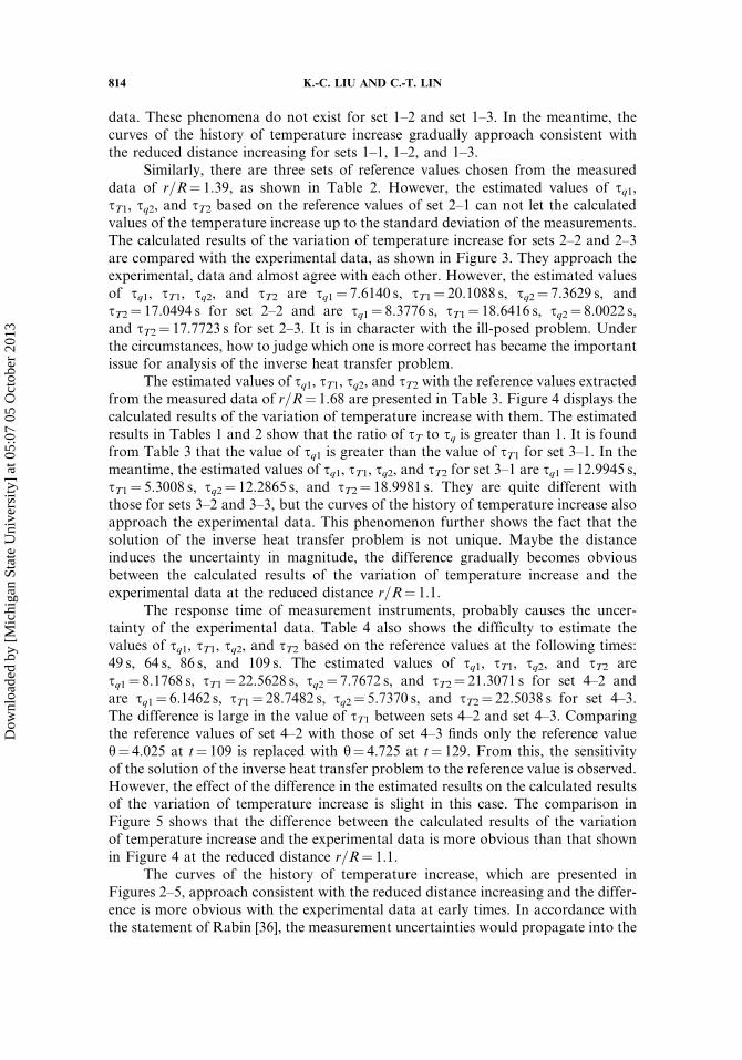
Similarly, there are three sets of reference values chosen from the measureddata of r=R¼ 1.39, as shown in Table 2. However, the estimated values of sq1,sT1, sq2, and sT2 based on the reference values of set 2–1 can not let the calculatedvalues of the temperature increase up to the standard deviation of the measurements.The calculated results of the variation of temperature increase for sets 2–2 and 2–3are compared with the experimental data, as shown in Figure 3. They approach theexperimental, data and almost agree with each other. However, the estimated valuesof sq1, sT1, sq2, and sT2 are sq1¼ 7.6140 s, sT1¼ 20.1088 s, sq2¼ 7.3629 s, andsT2¼ 17.0494 s for set 2–2 and are sq1¼ 8.3776 s, sT1¼ 18.6416 s, sq2¼ 8.0022 s,and sT2¼ 17.7723 s for set 2–3. It is in character with the ill-posed problem. Underthe circumstances, how to judge which one is more correct has became the importantissue for analysis of the inverse heat transfer problem.
The estimated values of sq1, sT1, sq2, and sT2 with the reference values extractedfrom the measured data of r=R¼ 1.68 are presented in Table 3. Figure 4 displays thecalculated results of the variation of temperature increase with them. The estimatedresults in Tables 1 and 2 show that the ratio of sT to sq is greater than 1. It is foundfrom Table 3 that the value of sq1 is greater than the value of sT1 for set 3–1. In themeantime, the estimated values of sq1, sT1, sq2, and sT2 for set 3–1 are sq1¼ 12.9945 s,sT1¼ 5.3008 s, sq2¼ 12.2865 s, and sT2¼ 18.9981 s. They are quite different withthose for sets 3–2 and 3–3, but the curves of the history of temperature increase alsoapproach the experimental data. This phenomenon further shows the fact that thesolution of the inverse heat transfer problem is not unique. Maybe the distanceinduces the uncertainty in magnitude, the difference gradually becomes obviousbetween the calculated results of the variation of temperature increase and theexperimental data at the reduced distance r=R¼ 1.1.
The response time of measurement instruments, probably causes the uncer-tainty of the experimental data. Table 4 also shows the difficulty to estimate thevalues of sq1, sT1, sq2, and sT2 based on the reference values at the following times:49 s, 64 s, 86 s, and 109 s. The estimated values of sq1, sT1, sq2, and sT2 aresq1¼ 8.1768 s, sT1¼ 22.5628 s, sq2¼ 7.7672 s, and sT2¼ 21.3071 s for set 4–2 andare sq1¼ 6.1462 s, sT1¼ 28.7482 s, sq2¼ 5.7370 s, and sT2¼ 22.5038 s for set 4–3.The difference is large in the value of sT1 between sets 4–2 and set 4–3. Comparingthe reference values of set 4–2 with those of set 4–3 finds only the reference valueh¼ 4.025 at t¼ 109 is replaced with h¼ 4.725 at t¼ 129. From this, the sensitivityof the solution of the inverse heat transfer problem to the reference value is observed.However, the effect of the difference in the estimated results on the calculated resultsof the variation of temperature increase is slight in this case. The comparison inFigure 5 shows that the difference between the calculated results of the variationof temperature increase and the experimental data is more obvious than that shownin Figure 4 at the reduced distance r=R¼ 1.1.
The curves of the history of temperature increase, which are presented inFigures 2–5, approach consistent with the reduced distance increasing and the differ-ence is more obvious with the experimental data at early times. In accordance withthe statement of Rabin [36], the measurement uncertainties would propagate into the
814 K.-C. LIU AND C.-T. LIN
Dow
nloa
ded
by [
Mic
higa
n St
ate
Uni
vers
ity]
at 0
5:07
05
Oct
ober
201
3
mathematical solution of heat transfer problem. Rabin [36] further indicated that thetemperature analysis based on a larger region is expected to be significantly moreaccurate and the effects of the measurement uncertainties on the prediction of tem-perature are more obvious at the early times. As a result, the present results arereasonable and the quality of the experimental data is important for the presentproblem. On the other hand, no matter what location the reference values are pickedfrom, the present calculated results of thermal response are close to the experimentaldata at various measurement locations. This phenomenon shows the efficiency ofthe present method for such a problem. In the meantime, the longer the distanceof the measurement location from the center is, the later the beginning of thermalresponse is. The behavior of finite propagation of thermal signal is graduallyreplaced by the diffusion behavior with the penetration distance of thermal signalincreasing. The above results enhance the features of the non-Fourier thermal beha-vior in the experimental data.
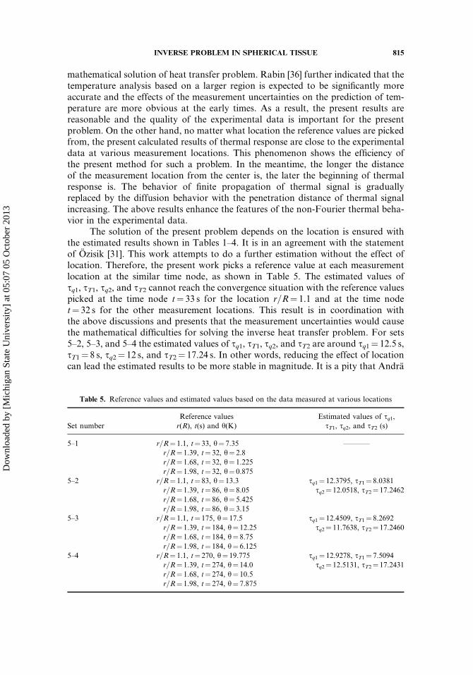
The solution of the present problem depends on the location is ensured withthe estimated results shown in Tables 1–4. It is in an agreement with the statementof Ozisik [31]. This work attempts to do a further estimation without the effect oflocation. Therefore, the present work picks a reference value at each measurementlocation at the similar time node, as shown in Table 5. The estimated values ofsq1, sT1, sq2, and sT2 cannot reach the convergence situation with the reference valuespicked at the time node t¼ 33 s for the location r=R¼ 1.1 and at the time nodet¼ 32 s for the other measurement locations. This result is in coordination withthe above discussions and presents that the measurement uncertainties would causethe mathematical difficulties for solving the inverse heat transfer problem. For sets5–2, 5–3, and 5–4 the estimated values of sq1, sT1, sq2, and sT2 are around sq1¼ 12.5 s,sT1¼ 8 s, sq2¼ 12 s, and sT2¼ 17.24 s. In other words, reducing the effect of locationcan lead the estimated results to be more stable in magnitude. It is a pity that Andra
Table 5. Reference values and estimated values based on the data measured at various locations
Set number
Reference values
r(R), t(s) and h(K)
Estimated values of sq1,sT1, sq2, and sT2 (s)
5–1 r=R¼ 1.1, t¼ 33, h¼ 7.35
r=R¼ 1.39, t¼ 32, h¼ 2.8
r=R¼ 1.68, t¼ 32, h¼ 1.225
r=R¼ 1.98, t¼ 32, h¼ 0.875
———–
5–2 r=R¼ 1.1, t¼ 83, h¼ 13.3
r=R¼ 1.39, t¼ 86, h¼ 8.05
r=R¼ 1.68, t¼ 86, h¼ 5.425
r=R¼ 1.98, t¼ 86, h¼ 3.15
sq1¼ 12.3795, sT1¼ 8.0381
sq2¼ 12.0518, sT2¼ 17.2462
5–3 r=R¼ 1.1, t¼ 175, h¼ 17.5
r=R¼ 1.39, t¼ 184, h¼ 12.25
r=R¼ 1.68, t¼ 184, h¼ 8.75
r=R¼ 1.98, t¼ 184, h¼ 6.125
sq1¼ 12.4509, sT1¼ 8.2692
sq2¼ 11.7638, sT2¼ 17.2460
5–4 r=R¼ 1.1, t¼ 270, h¼ 19.775
r=R¼ 1.39, t¼ 274, h¼ 14.0
r=R¼ 1.68, t¼ 274, h¼ 10.5
r=R¼ 1.98, t¼ 274, h¼ 7.875
sq1¼ 12.9278, sT1¼ 7.5094
sq2¼ 12.5131, sT2¼ 17.2431
INVERSE PROBLEM IN SPHERICAL TISSUE 815
Dow
nloa
ded
by [
Mic
higa
n St
ate
Uni
vers
ity]
at 0
5:07
05
Oct
ober
201
3
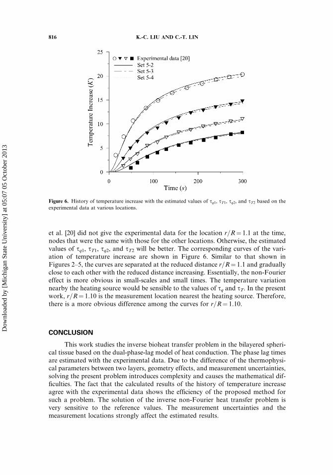
et al. [20] did not give the experimental data for the location r=R¼ 1.1 at the time,nodes that were the same with those for the other locations. Otherwise, the estimatedvalues of sq1, sT1, sq2, and sT2 will be better. The corresponding curves of the vari-ation of temperature increase are shown in Figure 6. Similar to that shown inFigures 2–5, the curves are separated at the reduced distance r=R¼ 1.1 and graduallyclose to each other with the reduced distance increasing. Essentially, the non-Fouriereffect is more obvious in small-scales and small times. The temperature variationnearby the heating source would be sensible to the values of sq and sT. In the presentwork, r=R¼ 1.10 is the measurement location nearest the heating source. Therefore,there is a more obvious difference among the curves for r=R¼ 1.10.
CONCLUSION
This work studies the inverse bioheat transfer problem in the bilayered spheri-cal tissue based on the dual-phase-lag model of heat conduction. The phase lag timesare estimated with the experimental data. Due to the difference of the thermophysi-cal parameters between two layers, geometry effects, and measurement uncertainties,solving the present problem introduces complexity and causes the mathematical dif-ficulties. The fact that the calculated results of the history of temperature increaseagree with the experimental data shows the efficiency of the proposed method forsuch a problem. The solution of the inverse non-Fourier heat transfer problem isvery sensitive to the reference values. The measurement uncertainties and themeasurement locations strongly affect the estimated results.
Figure 6. History of temperature increase with the estimated values of sq1, sT1, sq2, and sT2 based on the
experimental data at various locations.
816 K.-C. LIU AND C.-T. LIN
Dow
nloa
ded
by [
Mic
higa
n St
ate
Uni
vers
ity]
at 0
5:07
05
Oct
ober
201
3
REFERENCES
1. L. Zhang, W. Dai, and R. Nassar, A Numerical Method for Obtaining an Optimal Tem-perature Distribution in a 3-D Triple-Layered Cylindrical Skin Structure Embedded witha Blood Vessel, Numer. Heat Transfer A, vol. 49, pp. 765–784, 2006.
2. J. Wren, D. Loyd, and M. Karlsson, Investigation of Medical Thermal Treatment using aHybrid Bioheat Model, Proceedings of the 26th Annual International Conference of theIEEE EMBS, San Francisco, CA, USA, September 1–5, 2004.
3. A. V. Luikov, Analytical Heat Diffusion Theory, Academic Press, New York, 1968.4. W. Kaminski, Hyperbolic Heat Conduction Equation for Material with a
Non-Homogenous Inner Structure, ASME J. Heat Transfer, vol. 112, pp. 555–560, 1990.5. A. M. Braznikov, V. A. Karpychev, and A. V. Luikova, One Engineering Method
of Calculating Heat Conduction Process, Inzhenerno Fizicheskii Zhurnal, vol. 28,
pp. 677–680, 1975.6. K. Mitra, S. Kumar, A. Vedavarz, and M. K. Moallemi, Experimental Evidence of
Hyperbolic Heat Conduction in Processed Meat, ASME J. Heat Transfer, vol. 117,
pp. 568–573, 1995.7. W. Roetzel, N. Putra, and S. K. Das, Experiment and Analysis for Non-Fourier Conduc-
tion in Materials with Non-Homogeneous Inner Structure, Int. J. Therm. Sci., vol. 42,pp. 541–552, 2003.
8. W. H. Yang, Thermal (Heat) Shock Biothermomechanical Viewpoint, J. Biomedical Engi.,vol. 115, pp. 617–621, 1993.
9. T. C. Shih, H. S. Kou, C. T. Liauh, and W. L. Lin, The Impact of Thermal Wave Char-acteristics on Thermal Dose Distribution During Thermal Therapy: A Numerical Study,Med. Physi., vol. 32, pp. 3029–3036, 2005.
10. S. Ozen, S. Helhel, and O. Cerezci, Heat Analysis of Biological Tissue Exposed to Micro-wave by using Thermal Wave Model of Bioheat Transfer, Burns, vol. 34, pp. 45–49, 2008.
11. K. C. Liu, Thermal Propagation Analysis for Living Tissue with Surface Heating, Int.J. Thermal Sci., vol. 47, pp. 507–513, 2008.
12. D. Y. Tzou, The Generalized Lagging Response in Small-Scale and High-Rate Heating,Int. J. Heat Mass Transfer, vol. 38, pp. 3231–3240, 1995.
13. S. Godoy and L. S. Garcıa-Colın, Nonvalidity of the Telegrapher’s Diffusion Equation inTwo and Three Dimensions for Crystalline Solids, Phys. Rev. E, vol. 55, pp. 2127–2131,1997.
14. C. Korner and H. W. Bergman, The Physical Ddefects of the Hyperbolic Heat Conduc-tion Equation, Appl. Phys. A, vol. 67, pp. 397–401, 1998.
15. T. J. Bright and Z. M. Zhang, Common Misperceptions of the Hyperbolic Heat Equation,J. Thermophys. and Heat Transfer, vol. 23, pp. 601–607, 2009.
16. P. J. Antaki, New Interpretation of Non-Fourier Heat Conduction in Processed Meat,ASME J. Heat Transfer, vol. 127, pp. 189–193, 2005.
17. K. C. Liu and H. T. Chen, Analysis for the Dual-Phase-Lag Bioheat Transfer duringMagnetic Hyperthermia Treatment, Int. J. Heat and Mass Transfer, vol. 52, pp. 1187–1192, 2009.
18. J. Zhou, Y. Zhang, and J. K. Chen, An Axismmetric Dual-Phase-Lag Bioheat Model forLaser Heating of Living Tissues, Int. J. Thermal Sci., vol. 48, pp. 1477–1485, 2009.
19. Y. Zhang, Generalized Dual-Phase Lag Bioheat Equations Based on NonequilibriumHeat Transfer in Living Biological Tissues, Int. J. Heat and Mass Transfer, vol. 52,
pp. 4829–4834, 2009.20. W. Andra, C. G. d’Ambly, R. Hergt, I. Hilger, and W. A. Kaiser, Temperature Distri-
bution as Function of Time Around a Small Spherical Heat Source of Local MagneticHyperthermia, J. Magnetism and Magnetic Materials, vol. 194, pp. 197–203, 1999.
INVERSE PROBLEM IN SPHERICAL TISSUE 817
Dow
nloa
ded
by [
Mic
higa
n St
ate
Uni
vers
ity]
at 0
5:07
05
Oct
ober
201
3
21. S. K. Kim and I. M. Daniel, Solution to Inverse Heat Conduction Problem in Nanoscaleusing Sequential Method, Numer. Heat Transfer A, vol. 44, pp. 439–456, 2003.
22. H. T. Chen and X. Y. Wu, Estimation of Heat Transfer Coefficient in Two-DimensionalHeat Conduction Problems, Numer. Heat Transfer B, vol. 50, pp. 375–394, 2006.
23. H. T. Chen and X. Y. Wu, Estimation of Surface Conditions for Nonlinear Inverse HeatConduction Problems using the Hybrid Inverse Scheme, Numer. Heat Transfer B, vol. 51,pp. 159–178, 2007.
24. Y. Favennec, Hessian and Fisher Matrices for Error Analysis in Inverse Heat ConductionProblems, Numer. Heat Transfer B, vol. 52, pp. 323–340, 2007.
25. S. K. Kim, Resolving the Final Time Singularity in Gradient Methods for Inverse HeatConduction Problems, Numer. Heat Transfer B, vol. 57, pp. 74–88, 2010.
26. H. T. Chen, S. Y. Peng, P. C. Yang, and L. C. Fang, Numerical Method for HyperbolicInverse Heat Conduction Problems, Int. Commun. in Heat and Mass Transfer, vol. 28,pp. 847–856, 2001.
27. C. Y. Yang, Direct and Inverse Solutions of Hyperbolic Heat Conduction Problems,J. Thermophys. and Heat Transfer, vol. 19, pp. 217–225, 2005.
28. C. Y. Yang, Estimation of the Period Thermal Conditions on the Non-Fourier FinProblem, Int. J. Heat and Mass Transfer, vol. 48, pp. 3506–3515, 2005.
29. C. H. Huang and H. H. Wu, An Inverse Hyperbolic Heat Conduction Problem in Esti-mating Surface Heat Flux by Conjugate Gradient Method, J. Phys. D: Appl. Phys.,vol. 39, pp. 4087–4096, 2006.
30. C. H. Huang and C. Y. Lin, Inverse Hyperbolic Conduction Problem in Estimating TwoUnknown Surface Heat Fluxes Simultaneously, J. Thermophys. and Heat Transfer, vol. 22,pp. 766–774, 2008.
31. M. N. Ozisik, Heat Conduction, John Wiley and Sons, New York, 1993.
32. D. Y. Tzou, Macro- to Microscale Heat Transfer: The Lagging Behavior, Taylor &Francis, Washington, DC, 1996.
33. H. G. Bagaria and D. T. Johnson, Transient Solution to the Bioheat Equation andOptimization for Magnetic Fluid Hyperthermia Treatment, Int. J. Hyperthermia,vol. 21, pp. 57–75, 2005.
34. S. Maenosono and S. Saita, Theoretical Assessment of FePt Nanoparticles as Heating Ele-ments for Magnetic Hyperthermia, IEEE Trans. on Magnetics, vol. 42, pp. 1638–1642,2006.
35. G. Honig and U. Hirdes, A Method for the Numerical Inversion of Laplace Transforms,J. Comp. Appl. Math., vol. 10, pp. 113–132, 1984.
36. Y. Rabin, A General Model for the Propagation of Uncertainty in Measurements intoHeat Transfer Simulations and its Application to Cryosurgery, Cryobiology, vol. 46,pp. 109–120, 2003.
818 K.-C. LIU AND C.-T. LIN
Dow
nloa
ded
by [
Mic
higa
n St
ate
Uni
vers
ity]
at 0
5:07
05
Oct
ober
201
3