Solution Methods for Quadratic Optimization

Robert M. Freund

April 1, 2004

c©2004 Massachusetts Institute of Technology.

1

1 Outline

• Active Set Methods for Quadratic Optimization

• Pivoting Algorithms for Quadratic Optimization

• Four Key Ideas that Motivate Interior Point Methods

• Interior-Point Methods for Quadratic Optimization

• Reduced Gradient Algorithm for Quadratic Optimization

• Some Computational Results

2 Active Set Methods for Quadratic Optimization

In a constrained optimization problem, some constraints will be inactive at the optimal solution, and so can be ignored, and some constraints will be active at the optimal solution. If we knew which constraints were in which category, we could throw away the inactive constraints, and we could reduce the dimension of the problem by maintaining the active constraints at equality.

Of course, in practice, we typically do not know which constraints might be active or inactive at the optimal solution. Active set methods are designed to make an intelligent guess of the active set of constraints, and to modify this guess at each iteration.

Herein we describe a relatively simple active-set method that can be used to solve quadratic optimization problems.

Consider a quadratic optimization problem in the format:

TQP : minimizex xT Qx + c x

s.t. Ax = b (1)

x ≥ 0 .

2

1 2

[ ] ( )

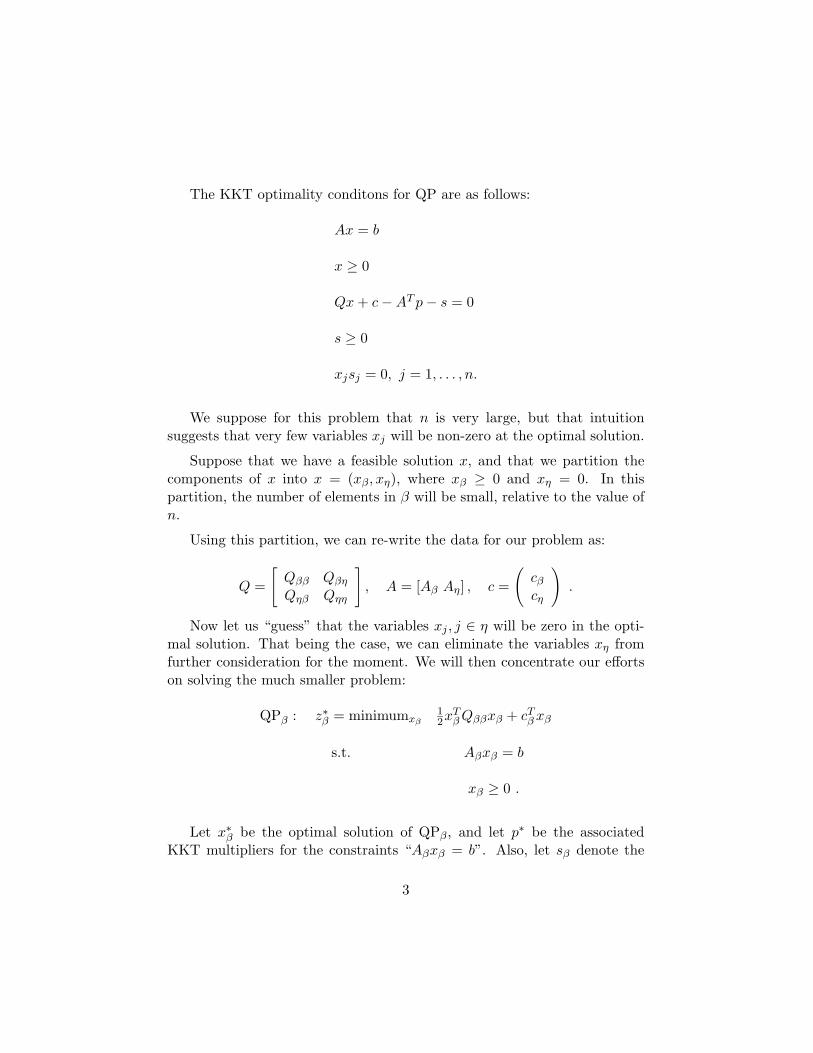
The KKT optimality conditons for QP are as follows:

Ax = b

x ≥ 0

Qx + c − AT p − s = 0

s ≥ 0

xjsj = 0, j = 1, . . . , n.

We suppose for this problem that n is very large, but that intuition suggests that very few variables xj will be non-zero at the optimal solution.

Suppose that we have a feasible solution x, and that we partition the components of x into x = (xβ , xη), where xβ ≥ 0 and xη = 0. In this partition, the number of elements in β will be small, relative to the value of n.

Using this partition, we can re-write the data for our problem as:

cβQ = Qββ Qβη , A = [Aβ Aη] , c = . Qηβ Qηη cη

Now let us “guess” that the variables xj , j ∈ η will be zero in the opti-mal solution. That being the case, we can eliminate the variables xη from further consideration for the moment. We will then concentrate our efforts on solving the much smaller problem:

QPβ : z ∗ β = minimumxβ

1 2xT T

β Qββxβ + cβ xβ

s.t. Aβxβ = b

xβ ≥ 0 .

∗Let xβ be the optimal solution of QPβ, and let p ∗ be the associated KKT multipliers for the constraints “Aβxβ = b”. Also, let sβ denote the

3

( )

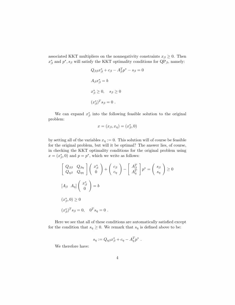
associated KKT multipliers on the nonnegativity constraints xβ ≥ 0. Then ∗ ∗ x and p , sβ will satisfy the KKT optimality conditions for QPβ, namely: β

∗ ∗ β p − sβ = 0Qββxβ + cβ − AT

∗ = bAβxβ

∗ x ≥ 0, sβ ≥ 0β

∗(xβ)T sβ = 0 .

∗We can expand x into the following feasible solution to the original β problem:

∗ x = (xβ , xη) = (xβ , 0)

by setting all of the variables xη := 0. This solution will of course be feasible for the original problem, but will it be optimal? The answer lies, of course, in checking the KKT optimality conditions for the original problem using

∗ ∗ x = (xβ , 0) and p = p , which we write as follows:

[ ]( ) ( ) [ ] ( ) x ∗ ATQββ Qβη β cβ − β p ∗ =

sβ+ ≥ 0 cη ATQηβ Qηη 0 η sη

∗ β[Aβ Aη]

x = b

0

∗(xβ , 0) ≥ 0

∗(xβ)T sβ = 0, 0T sη = 0 .

Here we see that all of these conditions are automatically satisfied except for the condition that sη ≥ 0. We remark that sη is defined above to be:

∗ ∗ sη := Qηβxβ + cη − AT η p .

We therefore have:

4

( )

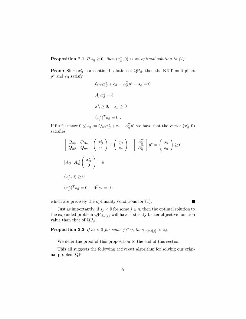
∗Proposition 2.1 If sη ≥ 0, then (xβ , 0) is an optimal solution to (1).

∗Proof: Since xβ is an optimal solution of QPβ , then the KKT multipliers ∗ p and sβ satisfy

∗ TQββxβ + cβ − Aβ p ∗ − sβ = 0

∗Aβxβ = b

∗ x ≥ 0, sβ ≥ 0β

∗(xβ)T sβ = 0 .

∗ T ∗If furthermore 0 ≤ sη := Qηβxβ + cη − Aη p ∗ we have that the vector (xβ , 0) satisfies

[ ]( ) ( ) [ ] ( ) ∗ Tx Aβ ∗ sβQββ Qβη β + cβ − T p = ≥ 0

Qηβ Qηη 0 cη Aη sη

∗ β[Aβ Aη]

x = b

0

∗(xβ , 0) ≥ 0

∗(xβ)T sβ = 0, 0T sη = 0 .

which are precisely the optimality conditions for (1).

Just as importantly, if sj < 0 for some j ∈ η, then the optimal solution to the expanded problem QPβ∪{j} will have a strictly better objective function value than that of QPβ.

Proposition 2.2 If sj < 0 for some j ∈ η, then zβ∪{j} < zβ.

We defer the proof of this proposition to the end of this section.

This all suggests the following active-set algorithm for solving our origi-nal problem QP:

5

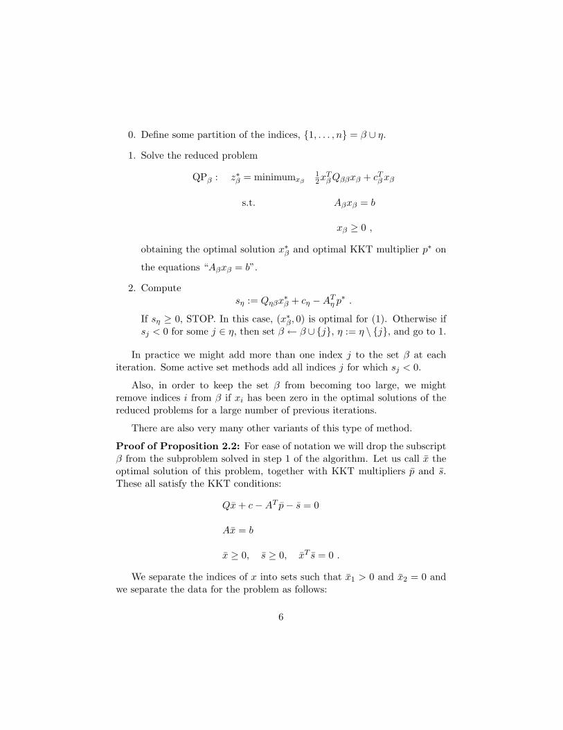
0. Define some partition of the indices, {1, . . . , n} = β ∪ η.

1. Solve the reduced problem

∗ 1 T TQPβ : z = minimumxβ xβ Qββxβ + cβ xββ 2

s.t. Aβxβ = b

xβ ≥ 0 ,

∗ ∗obtaining the optimal solution x and optimal KKT multiplier p onβ

the equations “Aβxβ = b”.

2. Compute ∗ ∗ sη := Qηβxβ + cη − AT

η p .

∗If sη ≥ 0, STOP. In this case, (xβ , 0) is optimal for (1). Otherwise if sj < 0 for some j ∈ η, then set β ← β ∪ {j}, η := η \ {j}, and go to 1.

In practice we might add more than one index j to the set β at each iteration. Some active set methods add all indices j for which sj < 0.

Also, in order to keep the set β from becoming too large, we might remove indices i from β if xi has been zero in the optimal solutions of the reduced problems for a large number of previous iterations.

There are also very many other variants of this type of method.

Proof of Proposition 2.2: For ease of notation we will drop the subscript β from the subproblem solved in step 1 of the algorithm. Let us call x the optimal solution of this problem, together with KKT multipliers p and s. These all satisfy the KKT conditions:

Qx + c − AT p − s = 0

Ax = b

¯ ¯x ≥ 0, s ≥ 0, xT s = 0 .

We separate the indices of x into sets such that ¯ x2 = 0 and x1 > 0 and we separate the data for the problem as follows:

6

[ ] ( )

[ ] ( )

[ ]

c1Q = Q11 Q12 , c = , A = [A1 A2] . Q21 Q22 c2

We then write the above system as:

¯Q11x1 + c1 − AT p = 01

¯Q21x1 + c2 − AT p − s2 = 02

A1x1 = b¯

x1 > 0, s2 ≥ 0 .

We now consider a new variable θ to add to this system. The data associated with this variable is q, δ, c, a, such that:

Q q c Q →

qT δ, c →

c, A → [A a]

Since this variable by supposition has a “reduced cost” that is negative, then the new data satisfies:

q x + ˆT ¯ c − a T p = −ε < 0 .

We will now show that this implies that there exists a feasible descent direction. The objective function of our problem and the formulas for the gradients of the objective function are:

[ ]( ) ( ) 1 x Tf(x, θ) = 2(x T , θ)

Q q + (c , c)

x Tq δ θ θ [ ]( ) ( )

c ∇f(x, θ) = Q q x

+Tq δ θ c ¯

x, 0) = qQ¯

x + ˆ= Q21x1 + c2 .

Q11x1 + c1

∇f(¯x + c ¯

T ¯ c T ¯q x + c

7

Invoking a nondegeneracy assumption, we assume that there exists a vector d1 for which A1d1 + a = 0. Then, since x1 > 0 we have that (x1, x2, θ) = (x1 + αd1, 0, α) ≥ 0, for α > 0 and small. Next we compute:

¯Q11x1 + c1 ¯

x, 0)T (d1, 0, 1) = (dT∇f(¯ 1 , 0, 1) Q21x1 + c2 q x + ˆT ¯ c

T ¯= (AT p)T d1 + q x + ˆ1 c

= −a T p + q T ¯ cx + ˆ = −ε < 0 .

Therefore (d1, 0, 1) is a feasible descent direction, and so the optimal objec-tive function value of the expanded problem is strictly less than that of the current problem.

3 Pivoting Algorithms for Quadratic Optimization

To facilitate the presentation, we will consider the following format for QP:

1 TQP : minimizex 2 xT Qx + c x

s.t. Ax ≥ b (π) (2)

x ≥ 0 (y)

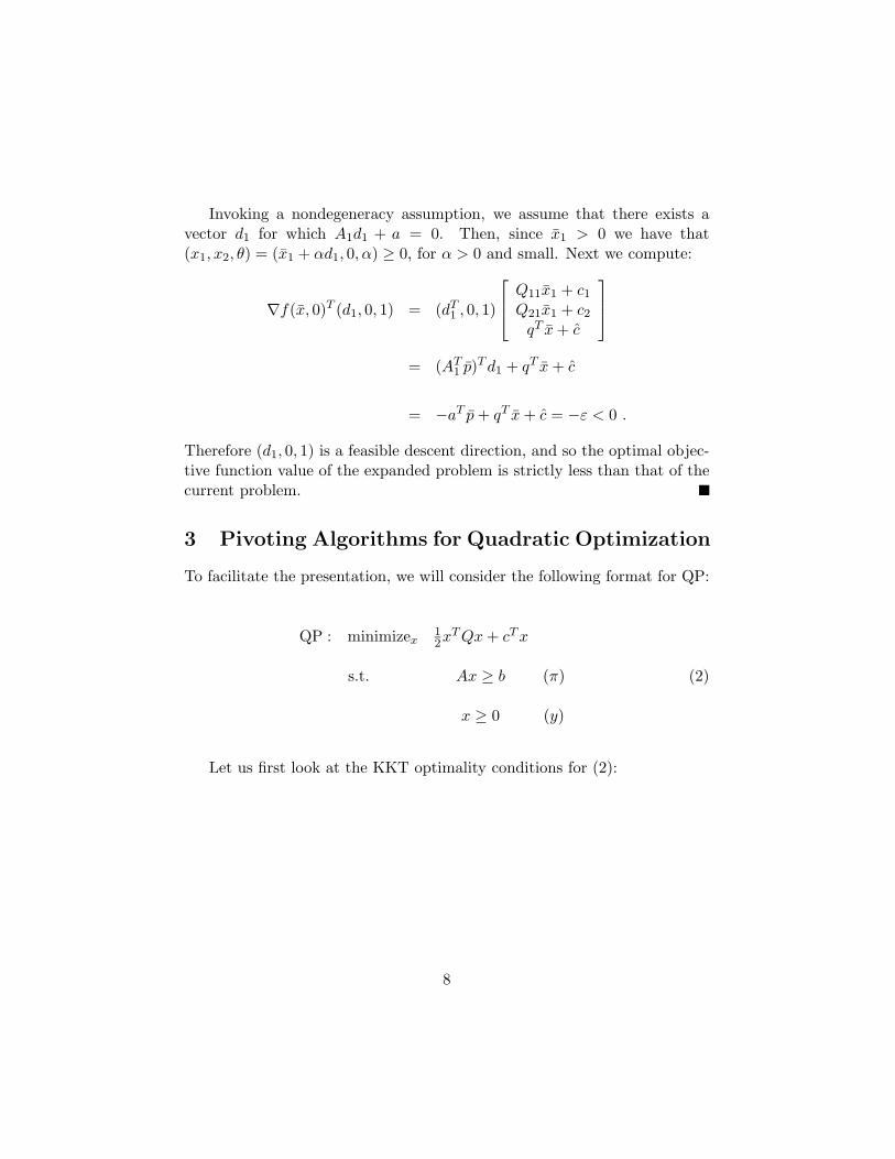
Let us first look at the KKT optimality conditions for (2):

8

s := Ax − b ≥ 0

x ≥ 0

Qx + c − AT π − y = 0

π ≥ 0

y ≥ 0

πisi = 0 i = 1, . . . , m

yj xj = 0 j = 1, . . . , n.

We can write the first five conditions in the form of a tableau of linear constraints in the nonnegative variables (y, s, x, π):

y s x π Relation RHS

I 0 −Q AT = c 0 I −A 0 = −b

and keeping in mind the nonnegativity conditions:

y ≥ 0 s ≥ 0 x ≥ 0 π ≥ 0

and the complementarity conditions:

yj xj = 0, j = 1, . . . , n, siπi = 0, i = 1, . . . , m.

This tableau has exactly (n + m) rows and 2(n + m) columns, that is, there are twice as many columns as rows. Therefore a basic feasible solution of this tableau will have one half of all columns in the basis.

We can find a basic feasible solution to this tableau (which has no objec-tive function row by the way!) by applying Phase I of the simplex algorithm. However, what we really want to do is to find basic feasible solution that is also “complementary” in the following sense:

9

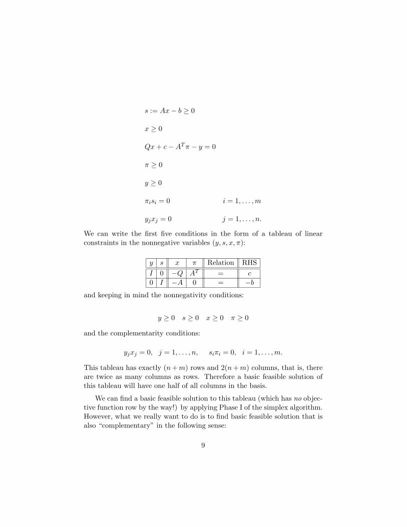
• Either yj is in the basis or xj is in the basis, but not both, j = 1, . . . , n,

• Either si is in the basis or πi is in the basis, but not both, i = 1, . . . , m.

Such a basic feasible solution will have the nice property that either yj = 0 or xj = 0, j = 1, . . . , n, and also si = 0 or πi = 0, i = 1, . . . , m. That is, a complementary basic feasible solution (CBFS) will satisfy the KKT conditions and so will solve QP.

One strategy for finding a CBFS is to add a nonnegative parameter θ and solve the following tableau:

y s x π Relation RHS

I 0 −Q AT = c + θe 0 I −A 0 = −b + θe

(Here e is the vector of ones of any appropriate dimension.) Now notice that for θ sufficiently large, that the RHS is nonnegative and so the complemen-tary basic solution:

y c + θe s −b + θe

= x

0

π 0

is a complementary basic feasible solution. The strategy then is try to start from this solution, and to drive θ to zero by a sequence of pivots that maintain a complementary basic feasible solution all the while. As it turns out, it is easy to derive pivot rules for such a strategy. The resulting algorithm is called the “complementary pivot algorithm”. It was originally developed by George Dantzig and Richard Cottle in the 1960s, and analyzed and extended by Carl Lemke, also in the 1960s.

We will not go over the specific pivot rules of the complementary pivot algorithm. They are simple but technical, and are easy to implement. What can we say about convergence of the complementary pivot algorithm? Just like the simplex method for linear optimzation, one can prove that the

10

complementary pivot algorithm must converge in a finite number of piv-ots (whenever the matrix Q is SPSD).

Regarding computational performance, notice that the tableau generally has twice the number of constraints and twice the number of variables as a regular linear optimization problem would have. This is because the primal and the dual variables and constraints are written down simultaneously in the tableau. This leads to the general rule that a complementary pivot algo-rithm will take roughly eight times as long to solve a quadratic program via pivoting as it would take the simplex method to solve a linear optimization problem of the same size as the primal problem alone.

Up until recently, most software for quadratic optimization was based on the complementary pivot algorithm. However, nowadays most software for quadratic optimization uses interior-point methods, which we will soon discuss.

4 Four Key Ideas that Motivate Interior Point Methods

We will work in this section with quadratic optimization in the following format:

QP : minimizex 1 2x TT Qx + c x

s.t. Ax = b (3)

x ≥ 0 .

4.1 A barrier function

The feasible region of (QP) is the set

F := {x | Ax = b, x ≥ 0} .

The boundary of F will be where one or more of the components of x is equal to zero. The boundary is composed of linear pieces, and is generally

11

∑

arranged in an exponentially complex manner. The simplex method takes explicit advantage of the linearity of the boundary, but can take a long time to solve a problem if there are exponentially many extreme points and edges to traverse. For this reason, we will take the curious step of introducing a barrier function B(x). A barrier function is any (convex) function defined on the interior of F and whose values go to infinity as the boundary is approached. That is:

• B(x) < +∞ for all x ∈ intF , and

• B(x) → ∞ as xj → 0.

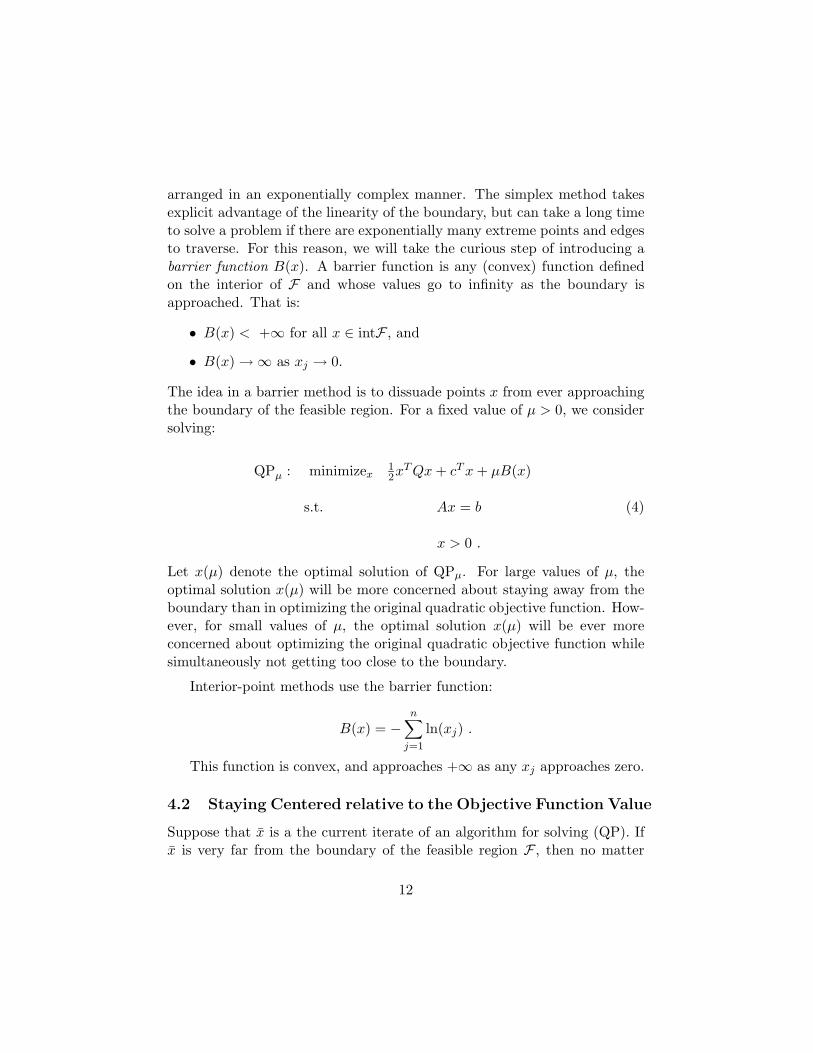
The idea in a barrier method is to dissuade points x from ever approaching the boundary of the feasible region. For a fixed value of µ > 0, we consider solving:

QPµ : minimizex 1 2x TT Qx + c x + µB(x)

s.t. Ax = b (4)

x > 0 .

Let x(µ) denote the optimal solution of QPµ. For large values of µ, the optimal solution x(µ) will be more concerned about staying away from the boundary than in optimizing the original quadratic objective function. How-ever, for small values of µ, the optimal solution x(µ) will be ever more concerned about optimizing the original quadratic objective function while simultaneously not getting too close to the boundary.

Interior-point methods use the barrier function:

n

B(x) = − ln(xj ) . j=1

This function is convex, and approaches +∞ as any xj approaches zero.

4.2 Staying Centered relative to the Objective Function Value

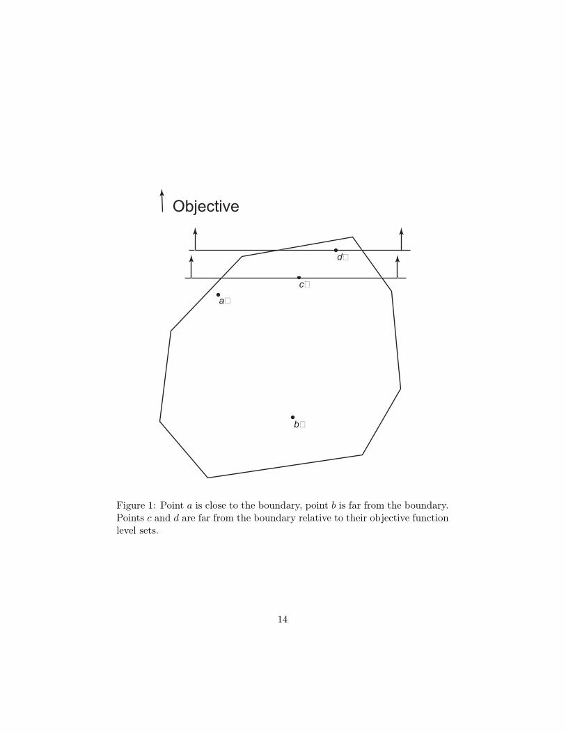
Suppose that x is a the current iterate of an algorithm for solving (QP). If x is very far from the boundary of the feasible region F , then no matter

12

∑

what direction we wish to go at the next iteration, we will have plenty of room to take a step, see Figure 1. However, since the optimal solution will generally lie on the boundary of the feasible region, we will want to keep the algorithm iterates as centered as possible for their objective function values. In the figure, point a is close to the boundary, point b is far from the boundary, and points c and d are far from the boundary relative to their objective function level sets.

Now consider the barrier version of our quadratic problem with the log-arithmic barrier:

n BPµ : minimizex

1 2x TT Qx + c x − µ

j=1 ln(xj )

s.t. Ax = b

x > 0 .

The objective function here will minimize the barrier term while also accounting for the original quadratic objective function. In this way, the solutions x(µ) of BPµ will be nicely centered relative to other feasible values x ∈ F with as good or better objective function values. Therefore the solutions x(µ) will be relatively far from the boundary for their objective function values.

4.3 Treating the KKT Conditions of the Barrier Problem as a Nonlinear Equation System

For a general barrier function B(x), our parameterized barrier problem is:

QPµ : minimizex 1 2x TT Qx + c x + µB(x)

s.t. Ax = b (5)

x > 0 .

Because the positivity conditions x > 0 will never be binding, the opti-mality conditions for this problem are:

13

Objective

d

c

a

b

Figure 1: Point a is close to the boundary, point b is far from the boundary. Points c and d are far from the boundary relative to their objective function level sets.

14

{ { }}

Ax = b

Qx + c − µ∇B(x) − AT p = 0

x > 0 .

This is a nonlinear equation system with n + m equations in the n + m variables (x, p). A generic algorithm for this system can be described as follows:

0. Start with some ¯ p.x > 0 and some ¯

1. If ‖A¯ x + c − µ∇B(¯x − b‖ ≤ ε and ‖Q¯ x) − AT p‖ ≤ ε for some small tolerance ε > 0, STOP. Otherwise go to Step 2.

2. Use some method, perhaps Newton’s method, to generate a desired step d = (dx, dp).

3. Compute a step-size that will maintain the positivity of the iterate value of x. Set r = 0.99, and compute:

¯θ = min 1, r min

xj .

∆xj <0 −∆xj

4. Re-set (¯ p) ← (¯x, ¯ x + θdx, p + θdp), and go to Step 1.

In this method, we check to see if we satisfy our nonlinear equations (to within some tolerance) in Step 1. We generate a presumably good direction d = (dx, dp) in Step 2. Although we would like to re-set (¯ p) ← (¯x, ¯ x + dx, p+ dp), we must ensure that our iterate values of x remain strictly positive. This is accomplished in Step 3. Note that the value r = 0.99 could be set to any positive value strictly less than 1.0 .

15

4.4 Newton’s Method

The last motivating idea in interior-point methods is Newton’s method. In its various forms, Newton’s method is a method for solving nonlinear equations by linearizing the equations at each iteration. Suppose that we wish to solve the equation system:

h1(x) = 0

. . . . . . . . . (6)

hn(x) = 0

where x = (x1, . . . , xn). We can write this succinctly as:

h(x) = 0

¯where h(x) = (h1(x), . . . , hn(x)). Let x denote the current iterate value. Then from Taylor’s theorem, we have:

h(¯ h(¯ x) + [H(¯x + ∆x) ≈ ˜ x + ∆x) := h(¯ x)] ∆x , (7)

where H(x) is the Jacobian matrix:

Hij (x) := ∂hi(x)

. ∂xj

Here the function ˜ x + ∆x) is the linear approximation of h(x) around the x. We can try to solve the system h(¯

h(¯point x = ¯ x + ∆x) = 0 by instead solving ˜ x + ∆x) = 0, which from (7) is: h(¯

h(¯ x)] ∆x = 0 . (8)x) + [H(¯

Solving (8) for ∆x, we obtain:

x)]−1 h(¯d := ∆x = − [H(¯ x) . (9)

The direction d is called the Newton direction or the Newton step. In a pure version of Newton’s method, we would set the next iteration value to be

xnew x + d .= ¯

16

( )

Newton’s method has remarkably fast convergence properties if the iter-ates lie near to the solution of the system. However, if the iterates are very far away from the solution of the system, Newton’s method typically does not have particularly good convergence properties.

5 Interior-Point Methods for Quadratic Optimiza­tion

5.1 The Central Path Equation System

For this section it will be most convenient to work with quadratic optimiza-tion in the following format:

QP : minimizex 1 2x TT Qx + c x

s.t. Ax = b (10)

x ≥ 0 .

Using the usual Lagrange duality constructions, we can derive the fol-lowing dual problem:

DP : maximizep,s,x bT p −1 2xT Qx

s.t. AT p + s − Qx = c

s ≥ 0 .

The following weak duality result follows by direct algebraic manipula-tion of the feasibility conditions:

Proposition 5.1 If x if feasible for (QP) and (p, s, x) is feasible for (DP), then the duality gap is:

1 T T1 x T Qx + c T x − bT p − x Qx = s x .

2 2

17

The KKT optimality conditons for QP are as follows:

Ax = b

x ≥ 0

AT p + s − Qx = c

s ≥ 0

xj sj = 0, j = 1, . . . , n.

The strong duality result is as follows:

Proposition 5.2 If x if feasible for (QP) and (p, s, x) is feasible for (DP), then x if optimal for (QP) and (p, s, x) is optimal for (DP) if and only if:

T s x = 0 .

Before we move on, let us introduce some notation that is used in interior-point methods. For vectors x and s, we denote:

x1 0

s1 0

1

X = . . . , S = . . .

, e = . . . .

0 xn 0 sn 1

Therefore, for example, x1s1 .

Xe = x, Se = s, XSe = . .

xns.

n

Now let us relax the KKT conditions above, by picking a value of µ > 0 and instead solve:

Ax = b, x > 0

AT p + s − Qx = c, s > 0

xj sj = µ, j = 1, . . . , n.

18

( )

∑

With our interior-point notation we can write this system as:

Ax = b, x > 0

AT p + s − Qx = c, s > 0

XSe = µe .

A solution (x, p, s) = (xµ, pµ, sµ) to this system for some value µ is called a point on the central path or central trajectory of the problem.

Proposition 5.3 If (x, p, s) is on the central path for some value µ > 0, then the duality gap is

1 T T1 x T Qx + c T x − bT p − x Qx = s x = nµ .

2 2

The proof of this proposition is a straightforward extension of the algebra of the system. The value of this proposition is that it shows that if we solve the system for smaller values of µ, then our duality gap will go to zero, and we will approximately solve our original problem.

We can also derive the central path by considering the following loga-rithmic barrier problem associated with QP for a given value of µ:

n BPµ : minimizex

1 xT Qx + cT x − µ ln(xj )2 j=1

s.t. Ax = b

x > 0 .

The KKT conditions for this logarithmic barrier problem are:

Ax = b, x > 0

Qx + c − µX −1e − AT p = 0 .

19

If we then define s := µX−1e > 0 and rearrange the above system, we obtain:

Ax = b, x > 0

AT p + s − Qx = c

XSe = µe .

Since x > 0 implies that s > 0, this is exactly the same system of equations we had derived earlier that define the central path.

5.2 The Newton Equation System

Suppose that we have a current “point” (actually a triplet) (¯ p, x, ¯ s) for which ¯ s > 0, and we are given a value of µ > 0. We want to compute a x > 0 and direction (∆x, ∆p, ∆s) so that (¯x +∆x, p+∆p, s+∆s) approximately solves the central path equations. We set up the system:

(1) A(x + ∆x) = b

(2) −Q(¯ p + ∆p) + (¯x + ∆x) + AT (¯ s + ∆s) = c

(3) ( ¯ X + ∆X)(S + ∆S)e = µe .

If we linearize this system of equations and rearrange the terms, we obtain the Newton equations for the current point (¯ p, x, ¯ s):

(1) A∆x = b − Ax =: r1

(2) −Q∆x + AT ∆p + ∆s = c + Qx − AT p − s =: r2

¯ ¯ ¯(3) S∆x + X∆s = µe − XSe =: r3

We refer to the solution (∆x, ∆p, ∆s) to the above system as the Newton direction at the point (¯ p, x, ¯ s).

20

{ { }}

{ { }}

( ) ( ) ¯

5.3 The Step-sizes

Given our current point (¯ p, x, ¯ s) and a given value of µ, we compute the Newton direction (∆x, ∆p, ∆s) and we update our variables by choosing a step-size θ, to obtain new values:

x, ˜ s) ← (¯ p, (˜ p, x, ¯ s) + θ(∆x, ∆p, ∆s) .

In order to ensure that ˜ s > 0, we choose a value of r satisfyingx > 0 and 0 < r < 1 (r = 0.99 is a common value in practice), and determine θ as follows:

¯θP = min 1, r min

xj

∆xj <0 −∆xj

sjθD = min 1, r min .

∆sj <0 −∆sj

We then set the step-size to be:

θ := min{θP , θD } .

5.4 Decreasing the Path Parameter µ

We also want to shrink µ at each iteration, in order to (hopefully) shrink the duality gap. The current iterate is (¯ p, x, ¯ s), and the current values satisfy:

T ¯x s µ ≈

n

We then re-set µ to

1 xT sµ ←

10 n,

where “10” is user-specified.

21

( ) ( )

5.5 The Stopping Criterion

We typically declare the problem solved when it is “almost” primal feasible, “almost” dual feasible, and there is “almost” no duality gap. We set our tolerance ε to be a small positive number, typically ε = 10−8, for example, and we stop when:

(1) ‖Ax − b‖ ≤ ε

x + AT p + ¯(2) ‖ − Q¯ s − c‖ ≤ ε

T ¯(3) s x ≤ ε

5.6 The Full Interior-Point Algorithm

a) Given (x0, p0, s0) satisfying x0 > 0, s0 > 0, and µ0 > 0, and r satisfying 0 < r < 1, and ε > 0. Set k ← 0.

b) Test stopping criterion. Check if:

(1) ‖Axk − b‖ ≤ ε

(2) ‖ − Qxk + AT pk + sk − c‖ ≤ ε

(3) (sk )T xk ≤ ε .

If so, STOP. If not, proceed.

1 (xk )T (sk )c) Set µ ←

10 n

d) Solve the Newton equation system:

(1) A∆x = b − Axk =: r1

(2) −Q∆x + AT ∆p + ∆s = c + Qxk − AT pk − sk =: r2

(3) Sk ∆x + Xk ∆s = µe − Xk Sk e =: r3

22

{ { }}

{ { }}

e) Determine the step-size:

k

θP = min 1, r min xj

∆xj <0 −∆xj

k

θD = min 1, r min sj

∆sj <0 −∆sj

θ = min{θP , θD } .

f) Update values:

k+1(x , pk+1, sk+1) ← (xk , pk , sk ) + θ(∆x,∆p, ∆s) .

Re-set k ← k + 1 and return to (b).

5.7 Solving the Newton Equations

We now show how to manipulate the Newton equations to yield some for-mulas for the solution of the Newton equation system. Given our current

x, ¯ s) for which ¯ s > 0, and a value of µ > 0, we wish to point (¯ p, ¯ x > 0 and solve the Newton equations below for (∆x,∆p, ∆s):

(1) A∆x = b − Ax =: r1

(2) −Q∆x + AT ∆p + ∆s = c + Qx − AT p − s =: r2

¯ ¯ ¯(3) S∆x + X∆s = µe − XSe =: r3

¯Pre-multiplying equation (2) by X, we obtain the following string of equations that derive from one another:

23

( ¯ )¯ ¯ ( ¯ ¯ ¯

( ( ) ¯ ¯ ( ¯ ¯ ¯

( ¯ ( )

( ¯

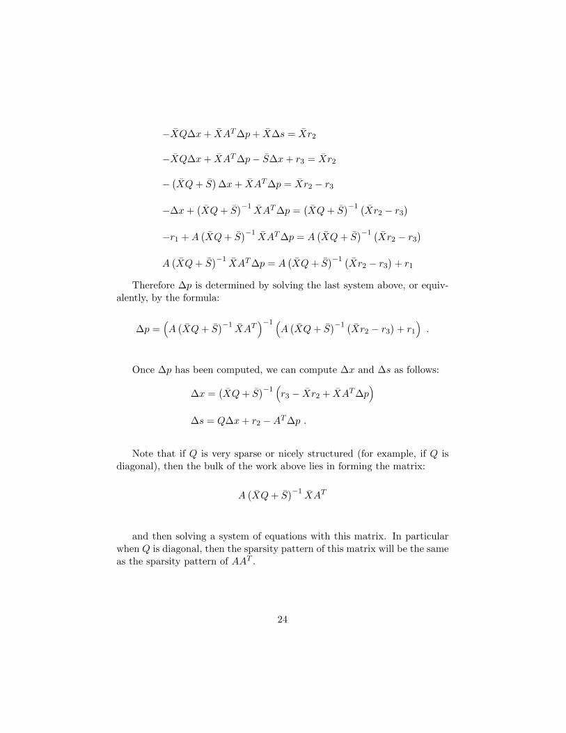
¯ ¯ ¯ ¯−XQ∆x + XAT ∆p + X∆s = Xr2

¯ ¯ ¯−XQ∆x + XAT ∆p − S∆x + r3 = Xr2

¯ ¯ ¯− XQ + S ∆x + XAT ∆p = Xr2 − r3

( ¯ )−1 ( ) −∆x + XQ + S )−1

XAT ∆p = XQ + S Xr2 − r3

( ¯ )−1 ( ))−1¯ ¯ ¯ ¯−r1 + A XQ + S XAT ∆p = A ( ¯ XQ + S Xr2 − r3

( ¯ )−1 ( ))−1¯ ¯ ¯ ¯ A XQ + S XAT ∆p = A ( ¯ XQ + S Xr2 − r3 + r1

Therefore ∆p is determined by solving the last system above, or equiv-alently, by the formula:

( ¯ )−1 ( ) ∆p = A XQ + S

)−1 XAT

)−1 A XQ + S Xr2 − r3 + r1 .

Once ∆p has been computed, we can compute ∆x and ∆s as follows:

¯ ¯ ¯∆x = XQ + S )−1

r3 − Xr2 + XAT ∆p

∆s = Q∆x + r2 − AT ∆p .

Note that if Q is very sparse or nicely structured (for example, if Q is diagonal), then the bulk of the work above lies in forming the matrix:

)−1 ¯ A XQ + S XAT

and then solving a system of equations with this matrix. In particular when Q is diagonal, then the sparsity pattern of this matrix will be the same as the sparsity pattern of AAT .

24

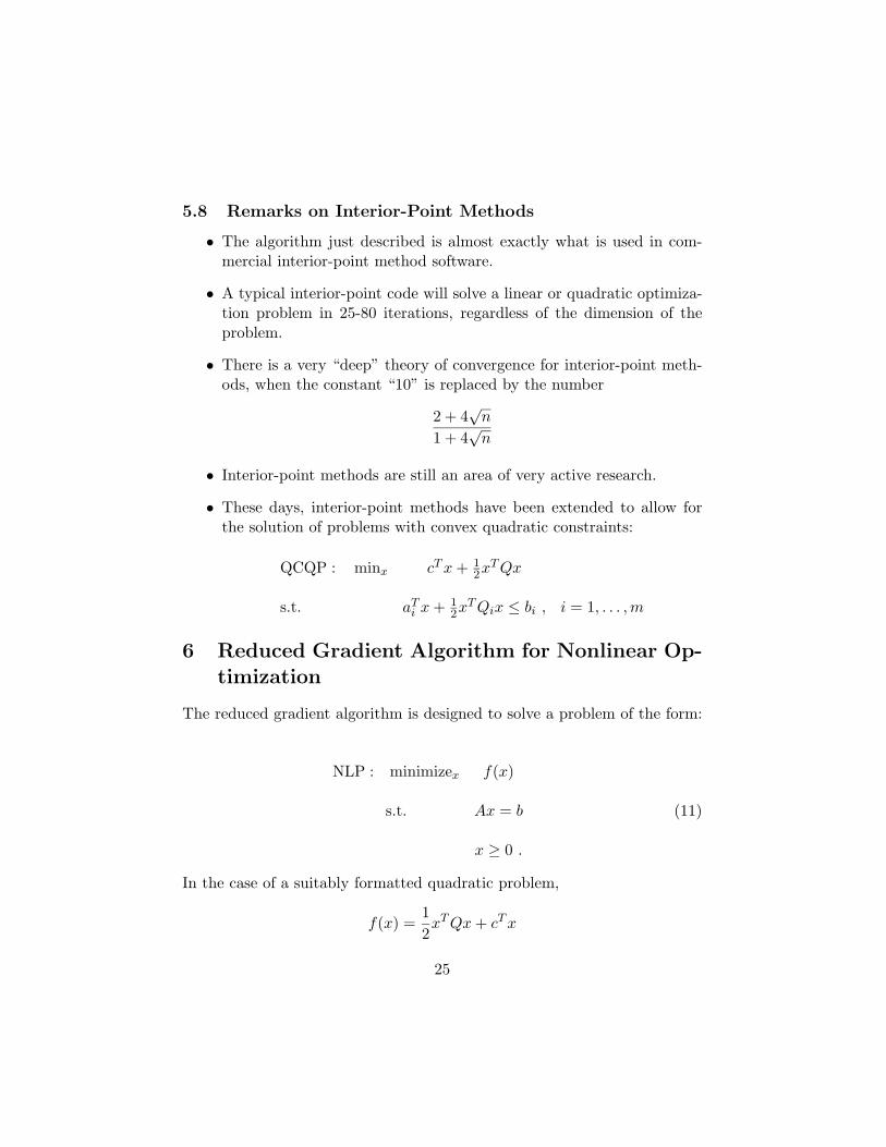
5.8 Remarks on Interior-Point Methods

• The algorithm just described is almost exactly what is used in com-mercial interior-point method software.

• A typical interior-point code will solve a linear or quadratic optimiza-tion problem in 25-80 iterations, regardless of the dimension of the problem.

• There is a very “deep” theory of convergence for interior-point meth-ods, when the constant “10” is replaced by the number

√2 + 4 n √1 + 4 n

• Interior-point methods are still an area of very active research.

• These days, interior-point methods have been extended to allow for the solution of problems with convex quadratic constraints:

1 2xT T QxQCQP : minx x +c

1 2xT

i x + T Qix ≤ bi , i = 1, . . . , ms.t. a

6 Reduced Gradient Algorithm for Nonlinear Op­timization

The reduced gradient algorithm is designed to solve a problem of the form:

NLP : minimizex f(x)

s.t. Ax = b (11)

x ≥ 0 .

In the case of a suitably formatted quadratic problem,

f(x) = 1 x T Qx + c T x

2

25

and ∇f(x) = Qx + c .

We will make the following assumptions regarding bases for the system “Ax = b, x ≥ 0”:

• For any basis β ⊂ {1, . . . , n} with |β| = m, Aβ is nonsingular.

• For any basic feasible solution (xβ , xη ) = (A−1b, 0) we have xβ > 0,β where here η := {1, . . . , n} \ β.

The reduced gradient algorithm tries to mimic certain aspects of the simplex algorithm.

At the beginning of an iteration of the reduced gradient algorithm, we have a feasible solution x for our problem NLP. Pick a basis β for which ¯xβ > 0. Remember that such a basis must exist by our assumptions, but that such a basis might not be uniquely determined by the current solution x. Set η := {1, . . . , n} \ β. Now invoke the equations of our system, which state that:

Aβ xβ + Aη xη = b

for any x = (xβ , xη ), and so we can write:

= A−1(b − Aη xη ) .xβ β

Since the basic variables are uniquely determined by the nonbasic variables above, we can substitute these into the formula for the objective function:

f(x) = f(xβ , xη ) = f(A−1(b − Aη xη ), xη ) .β

We therefore can define our reduced objective function to be:

h(xη ) = f(A−1(b − Aη xη ), xη ) .β

The gradient of the reduced objective function is called the reduced gradient, and has the following formula:

∇h(xη ) = ∇fη (A−1(b − Aη xη ), xη ) − AT η A

−T ∇fβ (A−1(b − Aη xη ), xη ) ,β β β

26

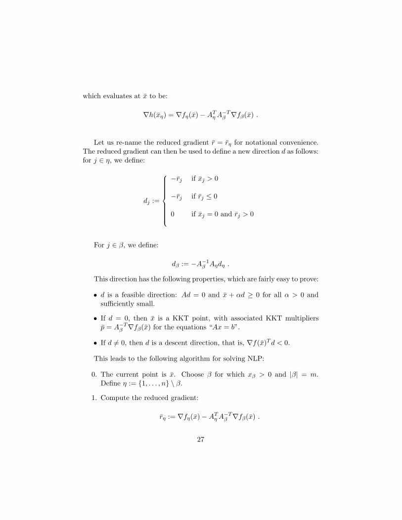
which evaluates at x to be:

∇h(¯ x) − AT x) .xη ) = ∇fη (¯ η A−T ∇fβ (¯β

r = ¯Let us re-name the reduced gradient ¯ rη for notational convenience. The reduced gradient can then be used to define a new direction d as follows: for j ∈ η, we define:

−rj if xj > 0 −rj if rj ≤ 0 dj := 0 if ¯ rj > 0 xj = 0 and

For j ∈ β, we define:

dβ := −A−1Aη dη .β

This direction has the following properties, which are fairly easy to prove:

¯• d is a feasible direction: Ad = 0 and x + αd ≥ 0 for all α > 0 and sufficiently small.

¯• If d = 0, then x is a KKT point, with associated KKT multipliers p = A−T ∇fβ (x) for the equations “Ax = b”.β

• If d � x)T d < 0.= 0, then d is a descent direction, that is, ∇f(¯

This leads to the following algorithm for solving NLP:

¯0. The current point is x. Choose β for which xβ > 0 and |β| = m. Define η := {1, . . . , n} \ β.

1. Compute the reduced gradient:

x) − AT x) .rη := ∇fη (¯ η A−T ∇fβ (¯β

27

{ }

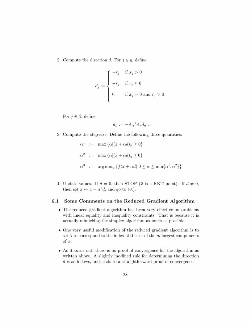
2. Compute the direction d. For j ∈ η, define:

−rj if xj > 0 −rj if rj ≤ 0 dj := 0 if ¯ rj > 0 xj = 0 and

For j ∈ β, define:

dβ := −A−1Aη dη .β

3. Compute the step-size. Define the following three quantities:

α1 := max {α|(x + αd)β ≥ 0}

α2 := max {α|(x + αd)η ≥ 0}

α3 := arg minα f (x + αd)|0 ≤ α ≤ min{α1, α2}

4. Update values. If d = 0, then STOP (¯ = 0, x is a KKT point). If d �then set ¯ x + α3d, and go to (0.). x ← ¯

6.1 Some Comments on the Reduced Gradient Algorithm

• The reduced gradient algorithm has been very effective on problems with linear equality and inequality constraints. That is because it is actually mimicking the simplex algorithm as much as possible.

• One very useful modification of the reduced gradient algorithm is to set β to correspond to the index of the set of the m largest components of x.

• As it turns out, there is no proof of convergence for the algorithm as written above. A slightly modified rule for determining the direction d is as follows, and leads to a straightforward proof of convergence:

28

∑ ∑ ∑ ∑ ∑ ∑

∑ ∑

For j ∈ η, define:

−rj if ¯ rj ≤ 0xj > 0 and −rj if ¯ rj ≤ 0 xj = 0 and

−¯ ¯ xj > 0 and dj := rj xj if ¯ rj > 0 0 if ¯ rj > 0 xj = 0 and

7 Some Computational Results

In this section we report some computational results on solving quadratic pattern classification problems. The problem under consideration is the dual of the pattern classification quadratic program with penalties for the case when we cannot strictly separate the points, namely D1:

T k k m k m1 k

D1 : maximizeλ,γ λi + γj − λia i − γj bj λia i − γj b

j 2

i=1 j=1 i=1 j=1 i=1 j=1

k m

s.t. λi − γj = 0 i=1 j=1 (12)

λi ≤ C i = 1, . . . , k

γj ≤ C j = 1, . . . , m

λ ≥ 0, γ ≥ 0 .

We refer to this problem as the REGULAR model. By defining the extra variables x:

29

∑ ∑

∑ ∑

( ) ∑ ∑

∑ ∑

k m

x := λia i − γj bj ,

i=1 j=1

we can re-write this model as:

k m TD2 : maximumλ,γ,x λi + γj − 1 x x2

i=1 j=1

k m s.t. x − λia

i − γj bj = 0

i=1 j=1

k m

λi − γj = 0 i=1 j=1

λi ≤ C i = 1, . . . , k

γj ≤ C j = 1, . . . , m

λ ≥ 0, γ ≥ 0

mλ ∈ �k , γ ∈ � .

We refer to this model as the EXPANDED model.

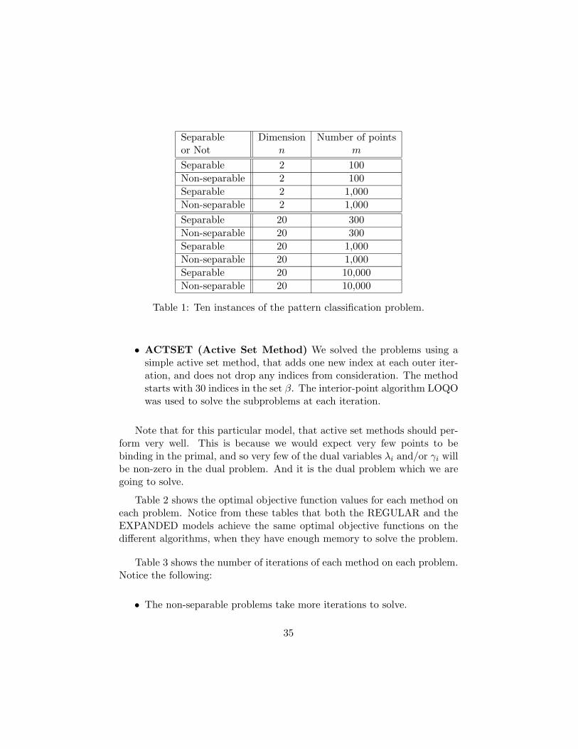
We solved ten instances of the pattern classification model that we cre-ated, whose main characteristics are as shown in Table 1. In solving these problem instances, we used the penalty value C = 1, 000.

The two-dimensional problems are illustrated in Figure 2, Figure 3, Fig-ure 4, and Figure 5.

We solved these instances using the following two algorithms:

• IPM (Interior-Point Method) We solved the problems using the software code LOQO, which is an interior-point algorithm implemen-tation for linear, quadratic, and nonlinear optimization.

30

−1 −0.8 −0.6 −0.4 −0.2 0 0.2 0.4 0.6 0.8 1 −1

−0.8

−0.6

−0.4

−0.2

0

0.2

0.4

0.6

0.8

1

Figure 2: Separable model with 100 points.

31

−1 −0.8 −0.6 −0.4 −0.2 0 0.2 0.4 0.6 0.8 1 −1

−0.8

−0.6

−0.4

−0.2

0

0.2

0.4

0.6

0.8

1

Figure 3: Non-separable model with 100 points.

32

−1 −0.8 −0.6 −0.4 −0.2 0 0.2 0.4 0.6 0.8 1−1

−0.8

−0.6

−0.4

−0.2

0

0.2

0.4

0.6

0.8

1

Figure 4: Separable model with 1,000 points.

33

−1 −0.8 −0.6 −0.4 −0.2 0 0.2 0.4 0.6 0.8 1−1

−0.8

−0.6

−0.4

−0.2

0

0.2

0.4

0.6

0.8

1

Figure 5: Non-separable model with 1,000 points.

34

Separable or Not

Dimension n

Number of points m

Separable 2 100 Non-separable 2 100 Separable 2 1,000 Non-separable 2 1,000

Separable 20 300 Non-separable 20 300 Separable 20 1,000 Non-separable 20 1,000 Separable 20 10,000 Non-separable 20 10,000

Table 1: Ten instances of the pattern classification problem.

• ACTSET (Active Set Method) We solved the problems using a simple active set method, that adds one new index at each outer iter-ation, and does not drop any indices from consideration. The method starts with 30 indices in the set β. The interior-point algorithm LOQO was used to solve the subproblems at each iteration.

Note that for this particular model, that active set methods should per-form very well. This is because we would expect very few points to be binding in the primal, and so very few of the dual variables λi and/or γi will be non-zero in the dual problem. And it is the dual problem which we are going to solve.

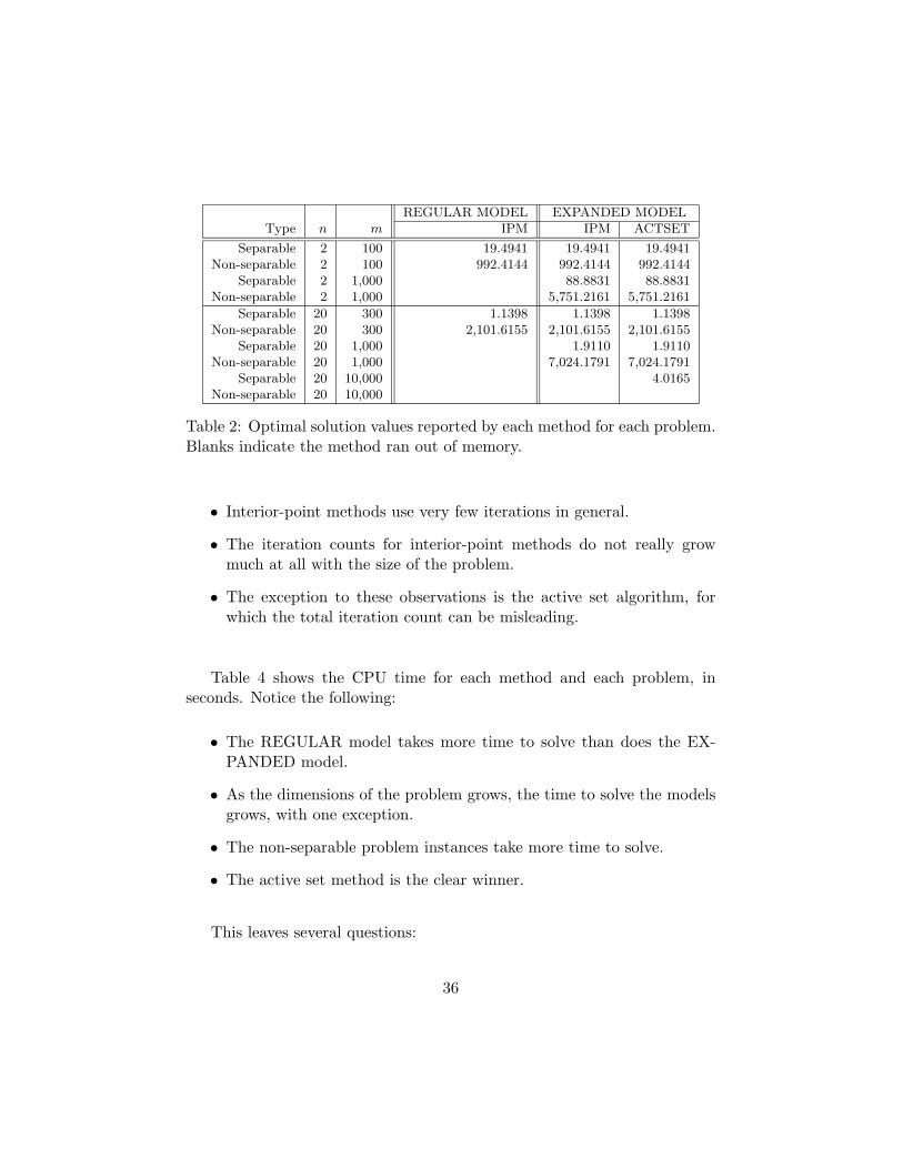
Table 2 shows the optimal objective function values for each method on each problem. Notice from these tables that both the REGULAR and the EXPANDED models achieve the same optimal objective functions on the different algorithms, when they have enough memory to solve the problem.

Table 3 shows the number of iterations of each method on each problem. Notice the following:

• The non-separable problems take more iterations to solve.

35

Type n m REGULAR MODEL EXPANDED MODEL

IPM IPM ACTSET

Separable 2 100 19.4941 19.4941 19.4941 Non-separable 2 100 992.4144 992.4144 992.4144

Separable 2 1,000 88.8831 88.8831 Non-separable 2 1,000 5,751.2161 5,751.2161

Separable 20 300 1.1398 1.1398 1.1398 Non-separable 20 300 2,101.6155 2,101.6155 2,101.6155

Separable 20 1,000 1.9110 1.9110 Non-separable 20 1,000 7,024.1791 7,024.1791

Separable 20 10,000 4.0165 Non-separable 20 10,000

Table 2: Optimal solution values reported by each method for each problem. Blanks indicate the method ran out of memory.

• Interior-point methods use very few iterations in general.

• The iteration counts for interior-point methods do not really grow much at all with the size of the problem.

• The exception to these observations is the active set algorithm, for which the total iteration count can be misleading.

Table 4 shows the CPU time for each method and each problem, in seconds. Notice the following:

• The REGULAR model takes more time to solve than does the EX-PANDED model.

• As the dimensions of the problem grows, the time to solve the models grows, with one exception.

• The non-separable problem instances take more time to solve.

• The active set method is the clear winner.

This leaves several questions:

36

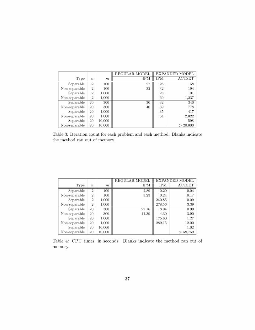
Type n m REGULAR MODEL EXPANDED MODEL

IPM IPM ACTSET

Separable 2 100 27 26 58 Non-separable 2 100 32 32 194

Separable 2 1,000 28 101 Non-separable 2 1,000 60 1,237

Separable 20 300 30 32 340 Non-separable 20 300 40 39 778

Separable 20 1,000 35 417 Non-separable 20 1,000 54 2,022

Separable 20 10,000 598 Non-separable 20 10,000 > 20,000

Table 3: Iteration count for each problem and each method. Blanks indicate the method ran out of memory.

Type n m REGULAR MODEL EXPANDED MODEL

IPM IPM ACTSET

Separable 2 100 2.89 0.20 0.04 Non-separable 2 100 3.23 0.24 0.17

Separable 2 1,000 240.85 0.09 Non-separable 2 1,000 278.56 3.39

Separable 20 300 27.16 8.04 0.99 Non-separable 20 300 41.39 4.30 3.90

Separable 20 1,000 175.60 1.27 Non-separable 20 1,000 289.15 12.00

Separable 20 10,000 1.02 Non-separable 20 10,000 > 58,759

Table 4: CPU times, in seconds. Blanks indicate the method ran out of memory.

37

• Why does the REGULAR model takes more time to solve than does the EXPANDED model?

• Why do the larger models run out of memory?

The answer to both of these questions probably has to do with the way LOQO handles the numerical linear algebra of forming and then factoring the Newton equation system at each interior-point iteration.

38