SOLUTION METHODS FOR PLANNING PROBLEMS IN

WIRELESS MESH NETWORKS

A THESIS

SUBMITTED TO THE DEPARTMENT OF INDUSTRIAL

ENGINEERING

AND THE GRADUATE SCHOOL OF ENGINEERING AND SCIENCE OF

BILKENT UNIVERSITY

IN PARTIAL FULFILLMENT OF THE REQUIREMENTS

FOR THE DEGREE OF

MASTER OF SCIENCE

By

Görkem Özdemir

August 2012

ii

I certify that I have read this thesis and that in my opinion it is full adequate, in scope

and in quality, as a dissertation for the degree of Master of Science.

___________________________________

Asst. Prof. Kağan Gökbayrak (Advisor)

I certify that I have read this thesis and that in my opinion it is full adequate, in scope

and in quality, as a dissertation for the degree of Master of Science.

___________________________________

Assoc. Prof. Emre Alper Yıldırım

I certify that I have read this thesis and that in my opinion it is full adequate, in scope

and in quality, as a dissertation for the degree of Master of Science.

______________________________________

Assoc. Prof. Bahar Yetiş Kara

Approved for the Graduate School of Engineering and Science

____________________________________

Prof. Dr. Levent Onural

Director of the Graduate School of Engineering and Science

iii

ABSTRACT

SOLUTION METHODS FOR PLANNING PROBLEMS

IN WIRELESS MESH NETWORKS

Görkem Özdemir

M.S. in Industrial Engineering

Supervisor: Asst. Prof. Kağan Gökbayrak

August 2012

Wireless Mesh Networks (WMNs) consist of a finite number of radio nodes. A subset of

these nodes, called gateways, has wired connection to the Internet and the non-gateway

nodes transmit their traffic to a gateway node through the wireless media in a multi-hop

fashion.

Wireless communication signals that propagate simultaneously within the same

frequency band may interfere with one another at a receiving node and may therefore

prevent successful transmission of data. In order to circumvent this problem, nodes on

the network can be configured to receive and send signals in different time slots and

through different frequency bands. Therefore, a transmission slot can be defined as a

pair of a certain frequency band and a specific time slot. In addition, by adjusting the

power level of a radio node, its transmission range can be modified.

Given a wireless mesh network with fixed node locations, demand rate at each node, and

maximum power level for each node, we study the problem of carrying the traffic of

each node to the Internet through the network. Our goal is to allocate capacities in

proportion to the demand of each node in such a way that the minimum ratio is

maximized. We propose a mixed integer linear programming (MILP) formulation to

select a given number of gateway locations among the nodes in the network, to

iv

determine the routing of the traffic of each node through the gateway nodes, to assign

transmission slots to each node in order to ensure no interference among wireless

signals, and to determine the transmission power levels. In our study, we adopt the

physical interference model, instead of the protocol interference, since this is more

realistic.

Since MILP formulation becomes computationally inefficient for larger instances; we

developed several different approaches. Then, we proposed a combinatorial optimization

model which successfully solves most of the instances. We tested our models and

methods in several data sets, and results are presented.

Keywords: Wireless Mesh Networks, Integer Programming, Gateway Selection,

Routing, Transmission Slot Assignment.

v

ÖZET

ÇOKGEN BAĞLANTILI KABLOSUZ AĞLARIN PLANLANMA PROBLEMLERİ

İÇİN ÇÖZÜM YAKLAŞIMLARI

Görkem Özdemir

Endüstri Mühendisliği Yüksek Lisans

Tez Yöneticisi: Yrd. Doç Dr. Kağan Gökbayrak

Ağustos 2012

Kablosuz Çokgen Bağlantılı Ağlar (KÇBA) sonlu sayıda telsiz düğümünden oluşur. Bu

düğümlerin ağ geçidi adı verilen bir alt kümesi İnternete doğrudan kablo ile bağlı iken,

ağ geçidi olmayan noktalar trafiklerini kablosuz ortamda birbirleri üzerinden ağ geçidine

aktarırlar.

Aynı frekans bandında aynı anda yayınlanan kablosuz iletişim sinyalleri alıcıda birbirine

karışabilir ve bu sebeple başarılı veri aktarımını engelleyebilir. Bu problemi engellemek

için ağdaki düğümler, farklı zaman dilimlerinde ve farklı frekanslar kullanacak şekilde

ayarlanabilir. Ayrıca, bir telsiz düğümünün güç seviyesi ayarlanarak aktarım aralığı

değiştirilebilir.

Bu çalışmada, verilen bir KÇBA için, düğümlerin lokasyonları, her düğümün talep oranı

ve en yüksek güç seviyesi bilindiğinde, düğümlerin trafiklerinin İnternete nasıl

taşınacağı problemine odaklandık. Amacımız, kapasiteleri her düğümün talebiyle

orantılı bir şekilde ve en küçük oranı en büyükleyerek bölüştürmektir. Bu sebeple,

verilen ağ düğümleri arasından ağ geçidi lokasyonlarını seçen, her nodun seçilen ağ

geçitleri üstünden trafiklerini belirleyen, kablosuz sinyallerin karışmasını önleyecek

şekilde veri aktarımının zaman aralıklarını belirleyen ve aktarımın güç seviyelerine karar

veren bir Karışık Tam Sayılı Program (KTSP) önerdik. Bu çalışmada, protokol karışma

modeli yerine daha gerçekçi olan fiziksel karışma modelini baz aldık.

vi

İlk önerilen KTSP formulasyonu büyük örnekler için olurlu sonuçlar elde

edemediğinden farklı yaklaşımlar üzerine yoğunlaştık. Önce bu model üzerine yapıla

eklemelerle yeni yöntemler geliştirirken, sonrasında bir kombinatoryal optimizasyon

modeli geliştirdik. Önerdiğimiz model ve yöntemleri farklı veri kümeleri üzerinde

yapılan deneylerin sonuçları üzerinden karşılaştırdık. Kombinatoryal eniyileme

modelinin diğerlerinden daha iyi sonuçlar verdiğini gözlemledik.

Anahtar Kelimeler: Kablosuz Çokgen Bağlantılı Ağlar, Tam Sayılı Programlama, Ağ

Geçidi Seçimi, Rotalama, Aktarım Zaman Aralığı Ataması.

vii

ACKNOWLEDGEMENT

The supervision of Kağan Gökbayrak throught the thesis process is kindly

acknowledged.

I would like to express my gratitude to Assoc. Prof. Emre Alper Yıldırım for his advises,

comments, and accepting to read this thesis.

I am grateful to Assoc. Prof. Bahar Yetiş Kara for not only accepting to read and

evaluate this thesis and sharing her comments, but also for being a guide for my whole

academic career.

I am grateful to Prof. İhsan Sabuncuoğlu, for detecting the talent besides the numerical

indicators. With his encouragement I have realized that I can be successful in academia

and made my career plans accordingly.

I am most thankful to my mom Sevil,dad Yalçın and sister Nazlı Şevval, for always

being there for me, their unconditional love, and supporting my every decision.

I would like to express my sincere gratitude to my dearest friends, who were by my side

during the most desperate days of the thesis process; Serasu Duran, Firat Kilci, Irfan

Mahmutogullari and Hasim Ozlu. I would also like to thank to my officemates Pelin

Çay, Sertalp Bilal Çay, Başak Yazar, Okan Dükkancı, Bengisu Sert and Nur Timurlenk

and all my friends I failed to mention for their kindness and morale support.

Finally, I would like to express my deepest and greatest gratitude for being there, being

by my side, supporting, encouraging me, being with me; to my love, Feyza Güliz

Şahinyazan. We have the basis, and the rest is just being built on it.

viii

TABLE OF CONTENTS Chapter 1: Introduction .................................................................................................. 1

Chapter 2: Wireless Mesh Networks .............................................................................. 3

2.1 Wireless Networks ................................................................................................... 3

2.2 Wireless Mesh Networks .......................................................................................... 4

2.3 Interference ............................................................................................................... 6

2.3.1 Protocol Model of Interference ................................................................................ 6

2.3.2 Physical Model of Interference ................................................................................ 7

2.4 Access Schemes ....................................................................................................... 8

2.4.1 Time Division Multiple Access (TDMA) ............................................................... 9

2.4.2 Frequency Division Multiple Access (FDMA) ...................................................... 9

2.4.3 Orthogonal Frequency Division Multiple Access (OFDMA) .............................. 9

Chapter 3: Literature Review & Problem Definition ................................................. 10

3.1 Review of the Related Literature on WMNs .......................................................... 10

3.2 Problem Definition ................................................................................................. 14

Chapter 4: Model Formulation ..................................................................................... 18

4.1 Assumptions ........................................................................................................... 18

4.2 Sets and Parameters ................................................................................................ 19

4.3 Decision Variables ................................................................................................. 20

4.4 Model Formulation ................................................................................................. 20

Chapter 5: Extensions to MILP Formulation ............................................................. 24

5.1 Valid Inequalities ................................................................................................... 24

5.1.1 A Logical Cut ............................................................................................................ 24

5.1.2 Link Analysis for Physical Interference ................................................................ 25

5.2 Maximum Number of Edges That Can Be Simultaneously Active ....................... 28

5.3 Two Solution Methods ........................................................................................... 29

Chapter 6: The Combinatorial Model ......................................................................... 31

6.1 The Model.............................................................................................................. 31

ix

6.2 A Logical Cut ........................................................................................................ 33

Chapter 7: Computational Analysis ............................................................................. 34

7.1 Data Sets ................................................................................................................. 34

7.2 Parameter Selection ................................................................................................ 35

7.3 Computational Experiments ................................................................................... 36

Chapter 7: Conclusion ................................................................................................... 39

BIBLIOGRAPHY .......................................................................................................... 41

APPENDIX ..................................................................................................................... 44

x

LIST OF FIGURES

Figure 2-1 Mesh Topology ................................................................................................ 4

Figure 2-2 Wireless mesh network, routers, clients and gateways .................................... 5

xi

LIST OF TABLES

Table 7-1 The Experimental Results Summary ............................................................... 37

1

Chapter 1

Introduction

A Wireless Mesh Network (WMN) is a wireless communication network in which the

nodes are not directly connected to the Internet with wire but send their traffic to a router

with wired connection on a multi-hop route. Since the required infra-structure is

relatively simple, deployment of WMNs are cost efficient.

However, increasing the share of wireless communication in the transmission of the

traffic on the network causes some extra problems. Simultaneous signals with the same

frequency may cause interference. This fact may cause the transmission of signals to

fail. Therefore, an efficiently working network can be obtained only with a priori

planning. On a WMN, basically the route, schedule, gateway placement and power

management decisions can be described as the planning problems.

2

In this study, those planning problems are addressed. The remaining of this thesis is

organized as follows:

In the next chapter, features of the WMNs are discussed. Then in Chapter 3, a brief

summary of the related literature is presented. The literature review is also followed by

the problem definition, in same chapter. Then, in Chapter 4, an MILP model that

addresses those mentioned planning problems jointly is proposed. Since this model is

difficult to solve, in Chapter 5, some extensions for this MILP formulation are

presented. In Chapter 6, a combinatorial optimization model is developed. Those models

are tested on several network data and the results are analyzed in Chapter 7. Finally, in

Chapter 8, the study is concluded with a brief summary and several suggestions for

extensions and future work.

3

Chapter 2

Wireless Mesh Networks

2.1 Wireless Networks

Wireless communication technology is being widely used since the last decade of 20th

century. The achievements in wireless technology gradually decrease the level of cabled

infrastructure needed in communication networks. This fact can be observed in the

progress of wireless communication protocols. There are mainly two wireless

networking protocols defined by the Institute of Electrical and Electronics Engineering

(IEEE). Those are; the older one, 802.11 Wireless Fidelity (Wi-Fi) and the relatively

recent one, 802.16 Worldwide Interoperability for Microwave Access (Wi-Max). While

Wi-Fi, which is commonly used in Wireless Local Area Networks (WLAN), is available

to use in relatively small areas (30 - 100 m), Wi-Max can cover larger areas, up to 50

km. Therefore, by utilizing Wi-Max, Metropolitan Area Network (MAN) applications

can be developed [1].

4

2.2 Wireless Mesh Networks

Wireless Mesh Networks (WMNs) are the family of wireless communication networks

that is based upon a mesh topology. An illustration of mesh topology is provided in

Figure 2.1. In a wireless network with that kind of a topology, mesh nodes in network

serve as a host to their clients and as a router to other mesh nodes. The main difference

between WMNs and the common wireless networks emerges from this second mission.

Rather than being connected to the wired system directly, the traffic is transmitted to the

node with wired connection, the gateway, on a route which may or may not consist of

multiple hops. Therefore, higher coverage of area and clients can be attained with less

wired infrastructure. This makes WMNs a relatively cost efficient alternative for

wireless communication.

Figure 2-1 Mesh Topology

According to Akyildiz et al., a wireless mesh network consists of two types of nodes,

mesh router (MR) and mesh client (MC). The mesh clients can be PCs, tablet computers,

mobile phones [2]. A mesh client is the device that the final user utilizes, and can be

mobile or static. On the other hand, mesh routers are statically placed, and as stated

5

above, both provide service to clients, and transmit the traffic of other mesh routers. A

typical wireless mesh network structure can be seen on Figure 2.2.

Figure 2-2 Wireless mesh network, routers, clients and gateways

The network topology is composed of mesh routers, nodes, and links between those

nodes. The conditions affecting the existence of a link are discussed in the following part

of this chapter. There is a certain capacity limiting the size of the data transmitted

through a link.

6

2.3 Interference

Due to the orbicular propagation of wireless signals, when traffic is transmitted through

a link, this may also affect remaining nodes as well. When a router sends signals to

another router, those signals are also received by all routers within a certain radius from

the sender router. If a router receives multiple signals at a time, none of them can be

processed. Therefore, the transmission of data between two nodes is possible only if all

of the other routers within a range of the destination node are silent during that time.

Accordingly, the communication between two nodes may disable some other links. This

phenomenon is called interference.

The interference issue is mathematically modeled by Gupta and Kumar with two

different approaches [3]. Those are, protocol model and physical model respectively.

2.3.1 Protocol Model of Interference

Protocol interference model is a relatively simplistic way of modeling interference issue

mathematically. In this model, transmission between two nodes, i and j, with positions

and can be successfully performed if for any other node k with position ,

which is also active simultaneously at the same frequency, the following inequality is

satisfied.

. (1)

In this inequality, corresponds to an auto-defensive guard like mechanism, “a

guard zone” as stated by Gupta and Kumar that precludes any transmission from

adjacent nodes.

7

2.3.2 Physical Model of Interference

As it can be figured out by the inequality (1), the protocol model for interference

considers the affects of other nodes individually, rather than evaluating the total noise

created by the whole on the network at that time and frequency. Additionally, the

protocol model does not include the power level of the signal being transmitted.

Combining those factors with the fact that the effect of distance on the signal noise is not

linear; a more realistic, but a complex way of modeling interference can be obtained.

Gupta and Kumar propose the following inequality for a transmission to be successfully

received:

Let S be the set of nodes active at a certain frequency and time, let γ denote the ambient

noise level, θ represent the Signal-to-Interference-Ratio (SIR), which is a threshold

value affecting the reception of signal. Then, the signal sent from node, i to node j, with

power can be received if

(2)

Here, α is the exponent by which the signal power decreases with distance. In other

words, it can be said that, the signal received at the destination node is inversely

proportional to the distance between the source and destination nodes to the power α.

Therefore, the reciprocal of the α exponent of the distance between two nodes i and j is

called the path loss between i and j and denoted by such that:

(3)

8

Then, (2) can be rewritten in the following form:

(4)

Then, assume that all nodes except i and j are inactive at some point in time. Then, the

signal with power can be transmitted between i and j if:

(5)

Therefore, denoting the maximum power that node i can transmit with ,

transmission between i and j can occur only if

(6)

Then, a link between two nodes exists if and only if (6) is satisfied. Defining

, we can rewrite (6) in the following form:

(7)

2.4 Access Schemes

Since interference allows only a limited part of the network to be active simultaneously,

different approaches have been developed for planning the traffic in wireless

communication networks. The traffic in WMNs can be sent using either decentralized

9

contention based or centralized non-contention based schemes. In contention based

schemes route or schedule are not a priori planned.

In non-contention based schemes, a central controller is required. In this study, we will

focus on Frequency Based Multiple Access and Time Based Multiple Access which are

both non-contention based schemes.

2.4.1 Time Division Multiple Access (TDMA)

TDMA is based on the logic that signals sent in different times do not create

interference. Therefore, a unit time, called a frame, is divided into time slots and

cyclically repeated. Interference is considered only within a time slot and if the number

of time slots is greater than or equal to the number of nodes, a trivial schedule can be

generated without considering the interference issue, by assigning each node a different

time slot to transmit its traffic. Nodes can utilize all available frequencies in their

assigned time slot.

2.4.2 Frequency Division Multiple Access (FDMA)

Interference can be avoided not only by dividing into slots but also sending signals on

different frequency bands. Wireless mesh routers are equipped to transmit and receive

signals from multiple channels. A node can send its traffic on the channels assigned to it

without any time limitations.

2.4.3 Orthogonal Frequency Division Multiple Access (OFDMA)

OFDMA is basically the combination of FDMA and TDMA. Time frame is divided into

slots and different frequencies can be used for transmission of different packages.

10

Chapter 3

Literature Review and Problem

Definition

3.1 Review of the Related Literature on WMNs

WMNs have been a popular research subject in the last decade. Since setting up a WMN

requires some critical and difficult decisions to be made, operations research methods

have been used in some part of those studies, especially the ones aiming to solve those

planning problems.

Gupta and Kumar [3] analyze the capacity of WMNs, and compare the difference

between randomly placed nodes and optimally placed nodes. They also define two

methods to model interference, since it directly affects the capacity of such networks.

Klasing et al. [4] model the bandwidth allocation problem on radio networks as a multi-

commodity flow problem, with a simplistic interference approach. In their study, they

11

define capacities depending on the interference relations between links, while

interference is defined as a binary relation considering the interaction between links in

pairs, instead computing the cumulative effect on simultaneous traffic at any link. They

name their formulation as Round Weighting Problem (RWP). To analyze the capacity

in more detail, Caillouet et al.[5] provide optimization based methods to determine the

theoretical capacity of a WMN, while working with a formulation analogous to the one

in Klasing’s study, in addition to providing a generic MILP model.

As the analysis by Gupta and Kumar [3] pioneers the research on capacity of WMNs,

different methods and solutions have been developed to cope with the interference issue,

besides analyzing the theoretical capacity. As an analogy to the access schemes

described in Chapter 1, the solution methods to overcome the limitations of interference

are mostly based on link scheduling or channel assignment.

Jain et al. [6] present methods on finding bounds on optimal throughput for a WMN,

under the protocol interference model. They prove that the problem of finding the

optimal throughput on a network under the protocol interference model is NP-Hard. On

the other hand, Kodialam and Nandagopal [7] propose algorithms for link scheduling

and channel assignment problem for both dynamic and static cases. Additionally, they

propose a mathematical constraint satisfaction model to determine bounds on optimal

solutions with a given objective.

Brar et al. [8], with the assumption of given traffic demands for links, propose a

computationally efficient algorithm to determine the schedule under the physical

interference model. Behzad and Rubin [9] present an MILP formulation which jointly

addresses link scheduling and power management decisions, to determine the minimum

schedule length. Since the model captures the power management decisions, the physical

interference model is used. They define the problem they address as Integrated Link

Scheduling and Power Control problem and give a proof that this problem is NP-

12

Complete. Capone and Carello [10] also provide an MILP formulation for the

scheduling problem of a given set of links and minimum number of packets to be

transmitted through each link. Power control and physical interference are included in

the model, while the objective is to minimize the required number of time slots. They

propose a column generation based solution approach for their formulation of the

problem. Papadaki and Friderikos [11] propose a dynamic programming approach to

schedule a given set of links, where each link has to be active for at least one time slot.

Similar to Brar et al. and Behzad and Rubin’s studies, Papadaki and Friderikos adopt the

physical interference model in their study.

All of those studies mentioned about link scheduling start with a given set of links to be

scheduled, i.e. the solution for routing part of the problem is taken as given, and they

deal with the problem of scheduling a given route, under the interference constraints.

Nevertheless, routing is also an important part of the problem, which directly effects the

potential limitations for the interference.

Raniwala et al [12] addresses the channel assignment and routing problems together,

under an IEEE 802.11 Wireless LAN setup. They provide an algorithm to obtain

solutions. Additionally, they present a proof that channel assignment problem is NP

Hard. Alicherry[13] et al. also address the channel assignment and routing problems

jointly. They provide an MILP formulation, and present algorithms based upon the LP

relaxation of the MILP. They assume that the multi path routing is possible and use the

protocol interference model.

Capone et al. [14] handles the routing, scheduling and channel assignment problems

together, and propose an MILP formulation. Similar to the approach in [10], they

propose a column generation based solution methodology.

In contrast with the MILP formulations and network or graph theory based algorithms,

meta-heuristic approaches to the planning problems of WMN are covered in only a few

13

studies. One such example is conducted by Badia et al. [15], proposing a genetic

algorithm to joint routing and link scheduling problem. Large instances for which MILP

formulations fails to give a solution can be handled with their algorithm.

The discussion in this chapter up to now covers a brief part of the WMN literature,

focusing on the studies on routing and scheduling methods. On the other hand, those

studies do not provide the answer to another strategic question for WMNs. As, having

less wired connection is a benefit of the WMN technology, appropriate choice of those

cable connections, namely the gateways, plays a crucial role in the performance of the

network. A significant part of the studies on WMNs are devoted to gateway selection

methods.

Chandra et al. [16] provide an MILP formulation for the problem of minimum number

of gateways, “Internet Transit Access Points” in the terminology they use, under quality

of service constraints, while also showing that this problem is NP-Hard. Moreover, they

propose a number of alternative algorithms for the same problem. Aoun et al. [17]

address the same problem, the gateway placement decision is handled while quality of

service constraints need to be satisfied. They provided a recursive dominating set

algorithm to decide on minimum number of gateways. On the other hand, neither [16]

nor [17] considers interference problem since routing and scheduling is not in the scope

of those studies.

The recent studies on gateway placement, however, take possible routing alternatives

and thus interference problem into account. Li et al. [18] address the gateway placement

problem with the objective of throughput maximization, and interference issue is also

embodied in the proposed ILP formulation. In this study, interference is considered with

the protocol model. In their recent paper, Targon et al. [19] provide an ILP formulation

to perform gateway placement that enables the network to satisfy the given demand with

minimum deployment cost. The formulation proposed in this study captures the

14

interference problem with the physical model. As interference is included, route and

schedule are also within the outputs of the provided formulation. Zhou et al. [20] address

the gateway placement problem with the objective of throughput maximization. In this

study, an algorithm that decides on the gateway places is proposed. Additionally, a non-

asymptotic analytical model is developed to determine the throughput depending on the

given gateway placement decision.

The studies discussed so far address some part of the decision problems with a

theoretical approach. On the other hand, there are already deployed wireless mesh

networks, at least for experimental purposes. The outputs of an early example of a

wireless mesh network deployed in Cambridge, Massachusetts are presented in Bicket et

al [21].

As mentioned at the very first sentence of this chapter, WMNs have been studied in an

extensive number of papers. The selection of studies presented here is mostly limited to

the ones addressing planning problems. One may find more information about WMNs in

the papers by Akyildiz et al [1] and Pathak and Dutta [22].

Here, a brief selection of studies on WMNs has been provided. In the literature, planning

issues regarding WMNs have been analyzed separately. The parts of the problem are

interrelated, and thus an integrated approach may be a good alternative, though creating

computational complexities. Such a holistic approach is studied in Uzunlar’s thesis [23].

In this study, an MILP formulation is provided, capturing gateway selection, routing,

transmission slot assignment and power management. Also, a gateway selection

heuristic is proposed.

3.2 Problem Definition

Centralized deployment of a WMN consists of a number of decisions to be made. At

first, the places of the routers should be determined. This is followed by the choice of

15

number and positions of the gateways. Then, the traffic among the network is planned.

This includes routing, selection of the links to be used, and transmission slot assignment,

by means of time slot and radio channel.

While planning the deployment of a WMN, either meeting the demand with minimum

deployment cost, or providing the best service quality under a pre-determined budget

can be aimed. The cost is directly related with the gateway decision; therefore, minimum

cost is reached with the minimum number of gateways, whereas a pre-determined

budget stands for the number of gateway points. In this study, the financial issues are not

analyzed and the number of gateways is taken as a given parameter.

Deployment of a WMN includes routing and transmission slot assignment planning in

two different levels. The first level is the transmission of traffic between MRs and the

Internet, and the second level is the interaction between MCs and MRs. In this study, we

address the planning of the traffic in the first level. For the second level, we simply

assume that a MC is served by the nearest MR.

On a WMN, MRs transmit their traffic to the Internet on multi-hop routes. Therefore,

each MR also transmits the traffic of other routers, for which they are on the specified

route. Each MR, using this multi-hop mechanism, reaches the Internet through a

gateway. The planning of this routing can be done in several different ways. A router

can send its traffic via multiple paths or a single path. The routing on the network may

or may not have a forest structure, which consists of a tree for each gateway point. To

avoid increasing computational complexity, we limit our analysis on single path routing

with forest structure. Therefore, division of traffic demand of a node is not allowed, and

similarly, traffic passing through a node cannot be sent by dividing into multiple routes.

A significant part of the previous researches on WMNs adopts the protocol interference

model that is described by Gupta and Kumar [3]. However, though this choice is better

considering the computational complexity, the simplicity of that model may lead to an

16

unrealistic representation of WMNs. Therefore, we adopt the physical interference

model that is also defined in Gupta and Kumar’s study.

For the transmission slots, the OFDMA scheme is adopted. Actually, TDMA, FDMA or

OFDMA are indifferent by means of computation as long as the number of transmission

slots is same. The number of transmission slots is the number of periods in a time frame

for TDMA, number of radio channels available for FDMA, and their product for

OFDMA. However, the number of radio channels that a router is equipped with is

limited, and dividing a unit time into a large number of periods may diverge from reality

since there may be, though negligibly little, some loss during the transition between

periods. Therefore, OFDMA would be a realistic choice. The time frame is taken as 1

second. Therefore, the determined schedule is repeated every second. The traffic

demand of routers and the transmission capacity of links are commonly denoted with the

unit of megabits per second (Mbps), thus choosing the time frame of 1 second is

convenient.

The power of transmitted signal directly affects the interference on network. For each

transmission to be performed, the appropriate power level should be determined.

Assuming that a router can change its power level a number of times in a second would

not be realistic. Therefore, for each router, the power level is taken to be the same within

the transmission slots. Any signal sent from this router is sent with this power level.

Our approach captures all of those sub-parts of the WMN planning problem jointly, and

aims to maximize the quality of service. The minimum service level provided to a node

is used as a measurement for quality of service, while service level of a node is defined

as the provided traffic-demand ratio for each node. Then, the problem we address can be

summarized as follows: Given the number and position of nodes, number of gateways to

be placed, traffic demands for each node, which selection of the gateways, route,

17

transmission slot assignment and associated power levels would maximize the minimum

service level provided among routers?

18

Chapter 4

Model Formulation

In the previous chapter, a description of the problem which is aimed to be solved is

presented. In this chapter, a mixed integer linear programming (MILP) formulation is

proposed for the WMN planning problem.

A WMN can be modeled as a network, with nodes and arcs, where each MR

corresponds to a node, and every possible connection forms an arc. The conditions under

which signal transmission between two nodes are possible are given in equation (6).

4.1 Assumptions

In the MILP formulation, the following statements are assumed to hold.

The locations of the MRs are known and static.

The WMN is deployed in accordance with IEEE 802.16 WIMAX protocol.

The MRs on the network are identical.

19

Each MR sends its traffic to the Internet on a single path, where the union of

those paths among routers forms a forest structure.

The transmission slots are based on OFDMA scheme.

Ambient noise power is static and equal at each point of the network.

A time frame is 1 second.

A router cannot switch between power levels within a time frame.

4.2 Sets and Parameters

Let be the number of nodes. Then, denotes the set of all nodes.

denotes the set of arcs. Then,

T denotes the number of time slots within a frame.

K denotes the number of radio channels available at each router.

The capacity of an arc is c Mbps.

The wired connection at a gateway node has a transmission capacity of α Mbps.

Number of gateways to be deployed is denoted by G.

is the vector of traffic demand for each node.

is the matrix of the received strength of signal with maximum power

between two nodes.

denotes the ambient noise level. Ambient noise is the existing noise on the

network without any signal.

is the SINR threshold value. A signal is received if the ratio of its power to the

cumulative noise on the network is higher than this value.

20

4.3 Decision Variables

4.4 Model Formulation

The developed model (WMN1) is quite similar to the one used in Uzunlar’s thesis [23],

with addition of channel assignments and some extra constraints for power control.

Actually, the extra constraints are the expressions of the assumption that a router cannot

switch between power levels within a second. The proposed model WMN1 is as follows:

21

s.t.

, (8)

(9)

,

(10)

, (11)

, (12)

, (13)

, (14)

, (15)

1 , (16)

(17)

22

(18)

, , , , (19)

(20)

The value used in constraint (17) is calculated as in equation (21):

(21)

This model finds a gateway placement, route, transmission slot assignment and power

levels for each transmission such that the minimum service level provided to any router

is maximized.

Constraint sets (6)-(13) focus on the routing and scheduling decisions. The constraint

sets (14)-(17) form the power management structure. The power management and

routing & scheduling decisions are linked by the physical interference constraint, (17).

And the last constraint states the condition of gateway selection.

The constraint (8) specifies the capacity of a link. At each time slot,

Mbps data can be

transmitted, therefore, flow on a link is limited with the multiplication of this capacity

with the number of transmission slots that there is traffic on that link.

The constraints (9) and (10) assure the balance of the flow and the capacity of wired

transmission at a gateway node. The traffic sent from a node which is not a gateway is

equal to the sum of incoming traffic and the provided service level times its demand. If it

23

is a gateway node, then the difference between incoming and outgoing traffic cannot

exceed the gateway capacity.

The constraint (11) forces every node to route its traffic, and also prevents a gateway

from sending its traffic to any other node. Constraint (12) guarantees that transmission

slots are assigned to only the links on the route. Therefore, this constraint forms the

connection between x and z variables.

A node can either receive or send traffic at any time. This is imposed by constraint (13).

The constraint (14) imposes that power is assigned only to the active links at any

transmission slot. Constraints (15) and (16) assure that the power level of a signal sent

from a node is equal to the determined power level of this node. Constraint sets (14),

(15) and (16) together, fix the power level of a link at a slot to 0, if that link is not active

at any transmission slot. Otherwise, it is fixed to the value.

The most complicated constraint at first sight seems to be the physical interference

constraint, (17). If a link is active at any transmission slot, then this constraint enforces

the physical interference condition stated in (2). Otherwise, the choice of ensures

this inequality to be a tautology.

Constraint (18) fixes the number of gateways. Constraint sets (19) and (20) are

integrality and non-negativity definitions of the decision variables.

This model is inadequate to solve planning problems. Therefore, a different approach, or

a better model is needed. In the following chapter, extensions for this formulation are

proposed. Then with those extensions, several methods are proposed. In the following

chapters, also another MILP formulation will be developed for the same problem.

24

Chapter 5

Extensions for MILP Formulation

The WMN1 formulation is inefficient to solve WMN planning problem. Therefore, it

needed to be improved with cuts and other approaches. In this chapter, we propose 3

valid cuts for this formulation, and an additional IP based approach to cope with the

difficulty created by interference problem.

5.1 Valid Inequalities

5.1.1 A Logical Cut

The current set of constraints enables, but does not force that every node is served. That

is, the solutions with zero service level are in the feasible set. However, in the definition

of problem, zero service level is not a desired solution. Then, those solutions can be

prevented to be mathematically feasible with appropriate set of inequalities.

Consider following inequality:

25

(22)

Then, if a link is on the decided route, transmission slot assignment to this link is forced.

Lemma 5.1: Inequality (22) defines a set of valid inequalities on the set of optimal

solutions of WMN1.

Proof: Let , be two vectors satisfying (11) and (18) and all

the remaining variables be equal to 0. Then, those variables form a feasible solution to

WMN1. Since this selection of variables does not satisfy (22), this solution is cut by

(22). On the other hand, consider an optimal solution. If there exists an optimal solution

with positive service level, then for all nodes i that are not gateway, by constraint (9) and

(10), outgoing flow should be positive. Then, by constraint (8), for some

should be positive. Then by constraints (11) and (12), the

corresponding value is 1, and (i,j) is the only link that is ever used, among the links

with source i. Then for remaining links with source i, Therefore, (22) is

satisfied. Then (22) does not cut any optimal solutions. Therefore (22) is valid on the set

of optimal solutions of WMN1.

5.1.2 Link Analysis for Physical Interference

Let and Then, assume that they are simultaneously active on the

same channel with associated power levels and

. Then by constraint (17), the

following two conditions hold:

(23)

(24)

26

Here, the cumulative noise term in (17) is omitted and this does not violate the

inequality, since it is a positive term in the right hand side of the inequality.

Then, by multiplying (24) by , we have:

(25)

Then, by substituting with the right hand side value of (24) in (25), we have:

(26)

Then, since

(27)

In the same way, multiplying (24) with and then substituting (23), we also have:

(28)

Therefore, we can say that, two links and can be simultaneously

active if (27) and (28) holds.

Then, let us define a new set, such that

or does not hold

Therefore, D is the set of link-pairs that cannot be active simultaneously. Then, the

following set of the inequalities can be added without causing any feasible solution to

become infeasible.

(29)

27

Lemma 5.2: The set of inequalities defined by (29) are valid for the set of optimal

solutions of WMN1.

Proof: By the above derivation, set D is defined as the set of conflicting edge pairs.

Therefore, there is no integer solution in which both of such edge pairs are active at the

same transmission slot. Hence, the inequalities defined by (29) do not cut any integer

solution. Thus, any optimal solution will satisfy (29)

In a similar fashion, such a relation can also be derived for link triples.

Then, let . Those three links can be active simultaneously if the

following conditions are satisfied.

(30)

(31)

28

(32)

Then, we can also define the set of conflicting triples:

or does not hold

Therefore, similarly, a valid inequality for link-triples can be added:

(33)

5.2 Computing The Maximum Number of Edges That Can Be

Simultaneously Active

If the maximum number of edges that can be simultaneously active, we can add this as a

new constraint to the WMN1 model. The formulation below gives the answer of this

question:

Assume we have only the routing and power variables. Then, we can maximize the sum

of routing variables subject to interference constraints. Additionally, the power variable

p does not have time and channel indices, therefore it’s denoted with

29

s.to

(34)

(35)

(36)

This model is named MaxEdge and gives the maximum number of edges that can be

simultaneously active, and also a selection of this number of such edges.

5.3 Two Solution Methods

In addition to solving WMN1 directly, two additional methods are proposed using the

above formulations. At first, it must be mentioned here that, from now on, WMN1 refers

to the generic MILP formulation with the addition of constraints (22) and (29).

WMNTriples is obtained with the addition of (33) to WMN1.

Additionally, the MaxEdge model can be used to generate all non-conflicting subsets of

. This can be obtained with iteratively solving MaxEdge with adding the constraint for

the selected edges such that:

30

Let w be the objective value of MaxEdge at the last iteration. Let the selected edges be

for

Then;

(37)

Solving MaxEdge iteratively, until the obtained objective is 1 will generate the all non-

conflicting subsets of A. Then, with this information, the required confliction constraints

can be added to WMN1 and thus the interference and power management constraints can

be omitted. By this way, WMNMaxEdge is obtained.

If the maximum number of edges that can be simultaneously active is less than or equal

to 3, than iteratively solving MaxEdge is unnecessary. Then, with being the

maximum number of edges that can be simultaneously active, we can add the following

constraint:

(38)

With the addition of (38) to WMNTriples if or to WMN1 if and omitting

the interference and power management constraints WMNMaxEdge for this case is

obtained.

31

Chapter 6

The Combinatorial Model

The set of all non-conflicting sets can be generated using MaxEdge. In our case, since

the buffers and buffer capacities of the routers are not taken into account, when is not an

important question, but how many times is the main question that we would like to

answer for each possible transmission. Building on this idea, we have developed an

MILP model, which allocates an available amount of transmission slots to non-

conflicting sets. The single route assumption is preserved in this setup. Since MaxEdge

model considers the physical interference while generating the sets, no additional power

management or interference constraints are required in such an approach.

6.1 The Model

The MaxEdge model gives us the information of all non-conflicting subsets of A. Then,

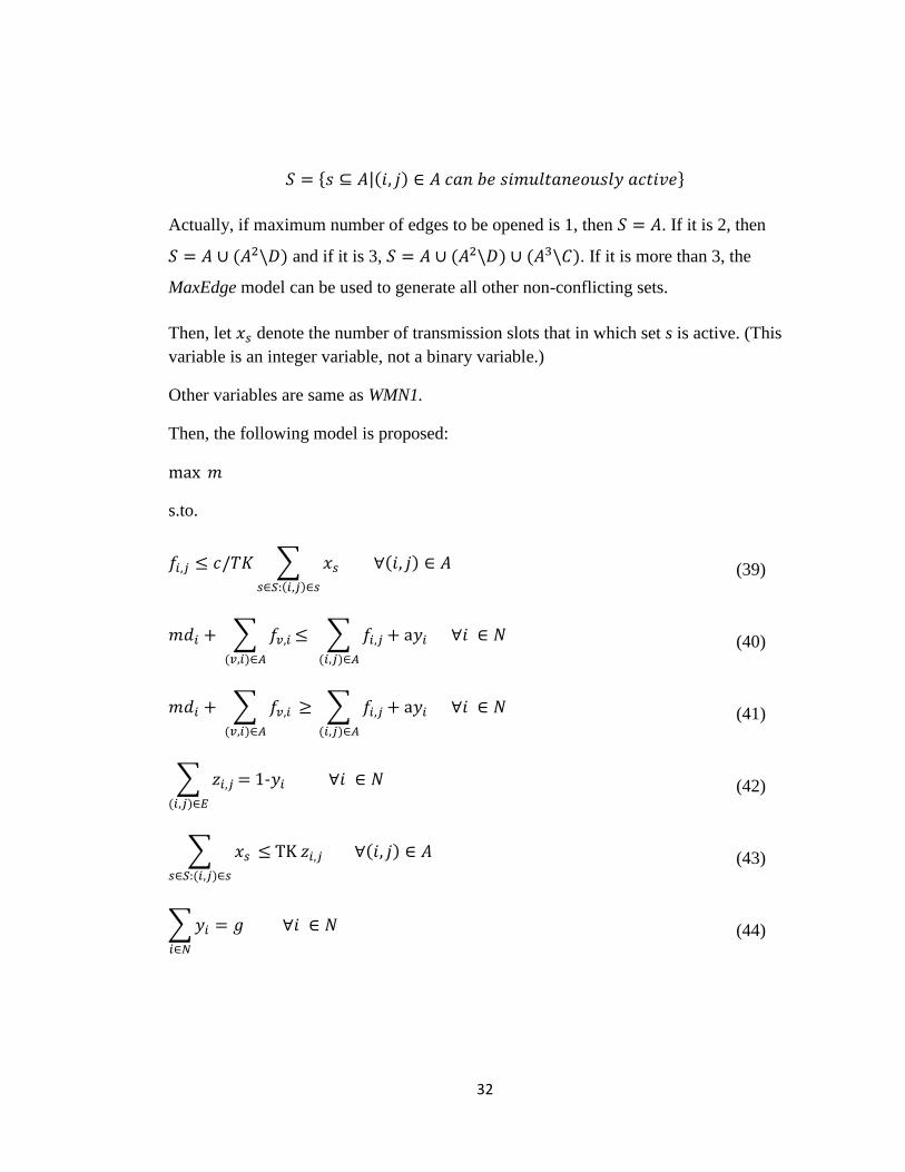
using this information, we can define the following set:

32

Actually, if maximum number of edges to be opened is 1, then . If it is 2, then

and if it is 3, . If it is more than 3, the

MaxEdge model can be used to generate all other non-conflicting sets.

Then, let denote the number of transmission slots that in which set s is active. (This

variable is an integer variable, not a binary variable.)

Other variables are same as WMN1.

Then, the following model is proposed:

s.to.

(39)

(40)

(41)

(42)

(43)

(44)

33

(45)

(46)

This model decides the number of times that the edges of set s are active. The only

constraint that can be considered as new is (43). This constraint ensures the connection

between the set selection and routing. Additionally, (39) has a minor difference with (8),

while having the same function. Finally, (45) states that the number of available

transmission slots is TK.

6.2 A Logical Cut

The following inequality ensures that if an edge is on the routing forest, than there is at

least one transmission slot in which a set including this edge is active:

(47)

The model with (51) is called WMNComb.

To sum up the last two chapters, WMN, WMNTriples, WMNMaxEdge and WMNComb

models are proposed. Those models are tested with several data structures. The results

are discussed in the next chapter.

34

Chapter 7

Computational Analysis

In the previous two chapters, a generic MILP formulation, an extension to this

formulation and a combinatorial MILP formulation is proposed.. To analyze the

affectivity of those methods, several computational experiments have been hold. In this

chapter, an analysis of the results of those computational experiments will be shared.

In order to test the developed methods, five different network datasets have been used.

Four of those data sets are generated according to the real population data of four

districts in Turkey: Uskudar, Cankaya, Beyoglu and Fatih. The fifth one is a network on

an 8x6 grid topology with randomly generated demand data.

7.1 Data Sets

The proposed methods are tested in five different networks.

Cankaya, Uskudar and 8x6 networks have grid topology while the nodes of Fatih and

Beyoglu networks are placed depending on the neighborhoods.

For an illustration, the figures of Cankaya and Uskudar networks can be seen in

Appendix 1A and 1B.

35

The node numbers for Uskudar, Cankaya, Beyoglu, Fatih and 8x6 are 15, 22, 24, 31 and

48 respectively. Therefore, Uskudar network can be considered as a small network,

while Cankaya is mid-small, Beyoglu is medium, Fatih is mid-large and 8x6 is a large

network. Actually, 8x6 network data is generated to challenge our methods with a very

large and difficult problem.

7.2 Parameter Selection

The problem requires some more data parameters besides the place and demand of nodes

to be set. SINR threshold value, ambient noise, the number of available channels in a

router and possible number of time slots in a frame should be detected.

The SINR threshold value and ambient noise level are determined in order to satisfy

connectivity in the network. It is assumed that each router can utilize 4 different radio

channels where a time frame can be divided into 8 and 16 time slots. Those assumptions

are chosen such that the technological capacities of the routers are not violated.

Since, in the assignment process, the number of transmission slots is the main factor that

makes difference, the configurations are named according to the multiplication of time

slots and number of channels. This multiplication is called TK number.

For deciding on the number of gateways, the WMNComb model is used with a different

objective. With fixing the service level to 1, the total number of gateways is minimized

and the 1 hr result of this model is used for each data as the number of gateways. Then,

the required number of gateways satisfying demand for Uskudar, Cankaya, Beyoglu,

Fatih and 8x6 are calculated as 2, 1, 2, 5 and 6 respectively.

The maximum number edges that can be simultaneously active for those networks are 1,

1, 2, 3 and 3 with the same order above. Note that, for the networks with this value less

than 3, WMNTriples is same as WMN.

36

7.3 Computational Experiments

For each network, WMN1, WMNTriples, WMNMaxEdge and WMNComb methods are

tested with TK values 32 and 64, with gateway numbers as mentioned above. In all of

the computational experiments, the time limit is set as 1 hr.

For Uskudar data, all of the methods have found the same solutions. However, while

WMNComb and WMNMaxEdge models prove the optimality of this solution, WMN

cannot decrease the bound in 1 hour.

For all of the configurations described, the formulations has been solved with Gurobi

5.0.1 on a CPU Intel i7 860(8 threads, 8M cache, 2.8 GHz).

The results of those experiments can be seen in Table 5.1. The detailed results can be

seen in Appendix 2.

For Cankaya network, with TK=32, the results are same as the Uskudar. The methods

give the same solution, while WMN cannot prove its optimality in 1 hr. For TK=64,

WMNComb and WMNMaxEdge have found the same solutions, which is slightly better

than the solution of WMN, and proven as optimal.

For all of the cases in which the optimality of a solution is proven by both WMNComb

and WMNMaxEdge, the CPU times of combinatorial model is less than WMNMaxEdge.

As the size of the network increases, the possibility of obtaining a proven optimal

solution in 1-hr decreases. On the other hand, the difference between the performance of

the methods become more obvious on the larger networks.

37

Table 7.1 The Experimental Results Summary

Configuration WMNComb WMNMaxEdge WMNTriples WMN

Uskudar

TK=32

1.07143 1.07143 1.07143 1.07143

Cankaya 1.25 1 1 1

Beyoglu 1.48515 1.48515 1.46648 1.46648

Fatih 1.25 0.9375 1 0.65217

8x6 1 0.53571 No Sol'n 0.57692

Uskudar

TK=64

1.18421 1.18421 1.18421 1.18421

Cankaya 1.25 1.21323 1.20535 1.20535

Beyoglu 1.75234 1.74419 1.64474 1.64474

Fatih 1.32353 0.57692 0.44776 0.9375

8x6 1.25 No Sol'n No Sol'n 0.625

For example, in Beyoglu network with TK=32, WMNComb and WMNMaxEdge models

find the same solution in 1-hr. However, the gap with the found best bounds are 1% for

WMNComb and 25% for WMNMaxEdge. The solution of WMN1 is worse than this

solution. While TK=64, the solution found by WMNComb is better than the other

methods, and it’s also the proven optimal solution.

For the Fatih network, the difference between the WMNComb and the other methods

increases. For TK=64, WmnComb finds more than twice of the solutions of other

methods. Also in 8x6 network, WmnComb’s solution is much better than the other

methods. Actually, WMNTriples cannot find a solution for 8x6 in 1-hr, and also

WMNMaxEdge fails to find a solution when TK=64. This is actually interesting, since

WMNMaxEdge is expected to perform better than WMN1. However, in a large network

like 8x6 grid network, the computation of non-conflicting triples cause extra complexity,

and the number of constrains increase dramatically. This, most probably, is the cause

why WMNMaxEdge fails to find a solution for this large network.

38

Another interesting point is that, with increasing TK value, WMNComb becomes slightly

easier, while this change decreases the performance of other methods. The reason for

that is the fact that, number of variables in WMNComb is independent of the other

parameters except the number of non-conflicting sets. However, the number of variables

increases in other methods when TK value is increased. For example, in 8x6 network,

there are 3040 non-conflicting edge sets, including the single edges. The cardinality of

edge set is 164. If we consider the x variables as analogous to each other between the

two main MILP formulations, in WMN1, there are 5248 x variables when TK=32, and

when TK duplicates, this value also duplicates. However, the number of x variables in

WMNComb remains as 3040, and the limitations by the constraints relax slightly since

the TK value increases.

To sum up, in all of the instances, WmnComb finds the best solution. The other methods

could not beat combinatorial model in any of the instances. Even if same solutions could

be reached, either solution times or the gaps indicate the superiority of combinatorial

model.

39

Chapter 8

Conclusion

This study covers the planning problems of WMNs. WMNs provide fast and cost

efficient network solutions. Since they do not require a complicated wired infra-

structure, WMNs are easy to deploy.

In the first chapter, general characteristics of WMNs are defined and described. A brief

summary of the literature about WMN planning problems is presented. Then our

problem is defined as jointly making the routing, gateway selection, transmission slot

assignment and power management decisions. In literature, most of the studies focus on

only some part of those decisions but do not address them jointly.

For the solution of WMN Planning problem, at first, a generic MILP model, WMN1, is

developed. Since this MILP formulation is computationally inefficient even in small

instances, different approaches are proposed. First, two sets of constraints are added into

WMN1 to improve the performance of the model. Then, a third inequality is added, and

40

with this addition, WMNTriples model is defined An easier MILP formulation is

developed to check the maximum number of edges that can be simultaneously active,

and generate all non-conflicting subsets of edge set A. By using this information, two

different methods are proposed, WMNMaxEdge and WMNComb.

Our proposed methods are tested on 5 different networks. One of those networks is

exteremely large and used for challenging our methods with such a case. The

comparison of the experimental runs showed that the combinatorial model, WMNComb,

performs better that the other models. In smaller instances, this can be observed in the

solution times, and in larger instances, this fact is obvious on the 1-hr solutions of the

methods. For small networks in which WMN1 cannot prove the optimality of a solution

in 1-hr, WMNComb solves to optimality in less than one second, and WMNMaxEdge

solves the problem, though not as fast as WMNComb. When the data size become larger,

WMNMaxEdge also become inefficient, even worse than WMN. However, in such cases,

WMNComb gives much better solutions in 1-hr. Therefore, to conclude, WMNComb

model is proposed as the main solution method presented in this thesis.

The WMN1 model is actually not a new formulation for the literature. It is quite similar

to Uzunlar’s model in [23]. On the other hand, the solution methods based on this

model, that is WMNMaxEdge is an important contribution of this thesis, along with the

MaxEdge model. On the other hand, the main contribution of this work is the

WMNComb model with its quite well performance in both small and large networks.

As a possible extension to this work, meta-heuristics for the WMN-Planning problem

can be developed. As it is mentioned in Chapter 3, there are very few studies in this area.

Additionally, considering the WMNComb model, column generation based approachs

can be a decent extension to this thesis.

41

BIBLIOGRAPHY

[1] WiMAX FAQ: What is FAQ? [Internet]. No date. [Cited 2012 July 13]. Available

from: http://www.wimax.com/wimax-faq/

[2] Akyildiz I, Wang X, Wang W. Wireless mesh networks: A survey. Computer

Networks. 2005; 47; 445-487.

[3] Gupta P, Kumar P.R. The Capacity of Wireless Networks. IEEE Transactions on

Information Theory. 2000; 46(2); 388-404.

[4] Klasing R, Morales N, Pérennes S. On the complexity of bandwidth allocation in

radio networks. Theoretical Computer Science. 2008; 406; 225-239.

[5] Caillouet C, Pérennes S, Rivano H. Framework for optimizing the capacity of

wireless mesh networks. Computer Communications. 2011; 34; 1645-1659.

[6] Jain K, Padhye J, Padmanabhan V, Qiu L. Impact of Interference on Multi-Hop

Wireless Network Performance. Wireless Networks. 2005; 11: 471-487.

[7] Kodialam M, Nandagopal T. Characterizing the Capacity Region in Multi-Radio

Multi-Channel Wireless Mesh Networks. Paper presented at: MobiCom 05, The

Eleventh Annual International Conference on Mobile Computing and Networking; 2005

August 28-September 2; Cologne, Germany.

[8] Brar G, Blough D, Santi P. Computationally Efficient Scheduling with the Physical

Interference Model for Throughput Improvement in Wireless Mesh Networks. Paper

presented at: MobiCom 06, The Twelfth Annual International Conference on Mobile

Computing and Networking; 2006 September 23-26; Los Angeles, California, USA.

42

[9] Behzad A, Rubin I. Optimum Integrated Link Scheduling and Power Control for

Multihop Wireless Networks. IEEE Transactions on Vehicular Technology. 2007; 56(1):

194-205.

[10] Capone A, Carello G. Scheduling Optimization in Wireless MESH Networks with

Power Control and Rate Adaptation. Paper presented at: 3rd Annual IEEE

Communications Society on Sensor and Adhoc Communications and Networks, 2006;

September 28, Reston, Virginia, USA.

[11] Papadaki K, Friderikos V. Approximate dynamic programming for link scheduling

in wireless mesh networks. Computers and Operations Research. 2008; 35; 3848-3859.

[12] Raniwala A, Gopalan K, Chiueh T. Centralized Channel Assignment and Routing

Algorithms for Multi-Channel Wireless Mesh Networks. Mobile Computing and

Communications Review. 2004; 8(2); 50-65.

[13] Alicherry M, Bhatia R, Li L. Joint Channel Assignment and Routing for

Throughput Optimization in Multi-radio Wireless Mesh Networks. Paper presented at:

MobiCom 05, The Eleventh Annual International Conference on Mobile Computing and

Networking; 2005 August 28-September 2; Cologne, Germany.

[14] Capone A, Carello G, Filippini I, Gualandi S, Malucelli F. Routing, scheduling and

channel assignment in Wireless Mesh Networks: Optimization models and algorithms.

Ad Hoc Networks. 2010; 8; 545-563.

[15] Badia L, Botta A, Lenzini L. A genetic approach to joint routing and link

scheduling for wireless mesh networks. Ad Hoc Networks. 2009; 7; 654-664.

[16] Chandra R, Qiu L, Jain K, Mahdian M. Optimizing the Placement of Internet TAPs

in Wireless Neighborhood Networks. Paper presented at: ICNP ’04, 12th

IEEE

International Conference on Network Protocols. 2004; October 5-8; Berlin, Germany.

43

[17] Aoun B, Boutaba R, Iraqi Y, Kenward G. Gateway Placement Optimization in

Wireless Mesh Networks With QoS Constraints. IEEE Journal on Selected Areas in

Communications; 2006; 24(11); 2127-2136.

[18] Li F, Wang Y, Li X, Nusairat A, Wu Y. Gateway Placement for Throughput

Optimization in Wireless Mesh Networks. Mobile Network Applications. 2008; 13; 198-

211.

[19] Targon V, Sanso B, Capone A. The joint Gateway Placement and Spatial Reuse

problem in Wireless Mesh Networks. Computer Networks. 2010; 54; 231-240.

[20] Zhou P,Wang X, Manoj B.S., Rao R. On Optimizing Gateway Placement for

Throughput in Wireless Mesh Networks. EURASIP Journal on Wireless

Communications and Networking. 2010; 1-12.

[21] Bicket J, Aguayo D, Biswas S, Morris R. Architecture and Evaluation of an

Unplanned 802.11b Mesh Network. Paper presented at: MobiCom 05, The Eleventh

Annual International Conference on Mobile Computing and Networking; 2005 August

28-September 2; Cologne, Germany.

[22] Pathak P.H, Dutta R. A survey of network design problems and joint design

approaches in wireless mesh networks. IEEE Communications Surveys and Tutorials.

2011; 13(3); 396-428.

[23] Uzunlar O. Joint Routing, Gateway Selection, Scheduling and Power Management

Optimization in Wireless Mesh Networks. [Master’s Thesis]. Bilkent University, 2011.

44

APPENDIX

45

APPENDIX 1A:Uskudar Network

12 13 14 15

8 9 10 11

4 5 6 7

1 2 3

0.4 0.6

0.8 0.5 1.2

0.8

0.7 0.7 1.1 1.7

0.7 1.9 1.1 0.8

2.0

The values on the nodes denote its demand.

46

APPENDIX 1B: Cankaya Network

19 20 21 22

14 15 16 17 18

9 10 11 12 13

4 5 6 7 8

1 2 3

0.4 0.7 0.4 0.3 0.3

0.3 0.1 0.8 0.2 0.3

0.4 0.3 0.2 0.6

0.2

0.6 0.6 0.1

0.2 0.3 0.3 0.9

The values on the nodes denote its demand.

47

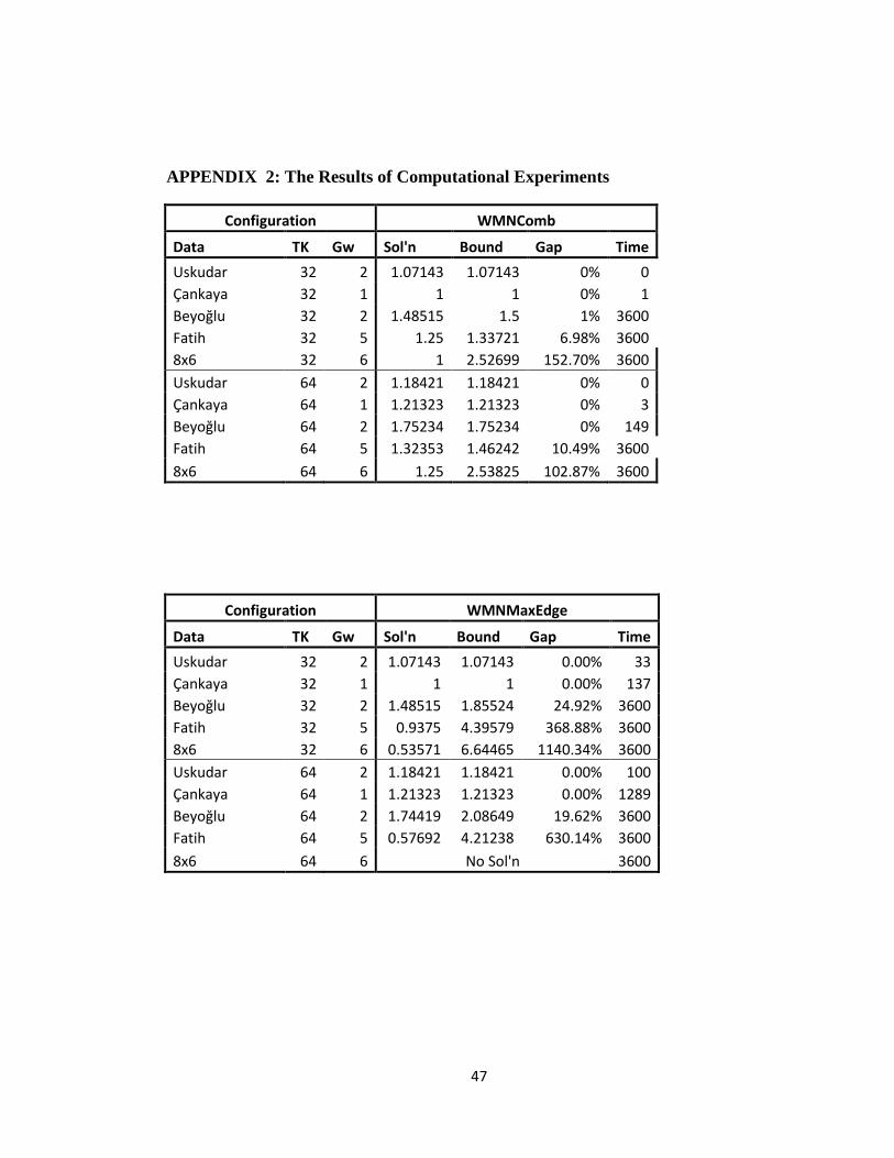
APPENDIX 2: The Results of Computational Experiments

Configuration WMNComb

Data TK Gw Sol'n Bound Gap Time

Uskudar 32 2 1.07143 1.07143 0% 0

Çankaya 32 1 1 1 0% 1

Beyoğlu 32 2 1.48515 1.5 1% 3600

Fatih 32 5 1.25 1.33721 6.98% 3600

8x6 32 6 1 2.52699 152.70% 3600

Uskudar 64 2 1.18421 1.18421 0% 0

Çankaya 64 1 1.21323 1.21323 0% 3

Beyoğlu 64 2 1.75234 1.75234 0% 149

Fatih 64 5 1.32353 1.46242 10.49% 3600

8x6 64 6 1.25 2.53825 102.87% 3600

Configuration WMNMaxEdge

Data TK Gw Sol'n Bound Gap Time

Uskudar 32 2 1.07143 1.07143 0.00% 33

Çankaya 32 1 1 1 0.00% 137

Beyoğlu 32 2 1.48515 1.85524 24.92% 3600

Fatih 32 5 0.9375 4.39579 368.88% 3600

8x6 32 6 0.53571 6.64465 1140.34% 3600

Uskudar 64 2 1.18421 1.18421 0.00% 100

Çankaya 64 1 1.21323 1.21323 0.00% 1289

Beyoğlu 64 2 1.74419 2.08649 19.62% 3600

Fatih 64 5 0.57692 4.21238 630.14% 3600

8x6 64 6 No Sol'n 3600

48

Configuration WMNTriples

Data TK Gw Sol'n Bound Gap Time

Uskudar 32 2 1.07143 6 460.00% 3600

Çankaya 32 1 1 1.15772 15.77% 3600

Beyoğlu 32 2 1.46648 1.83349 25.03% 3600

Fatih 32 5 1 4.09174 309.17% 3600

8x6 32 6 No Sol'n 3600

Uskudar 64 2 1.18421 6 406.67% 3600

Çankaya 64 1 1.20535 1.29972 7.83% 3600

Beyoğlu 64 2 1.64474 4.45158 170.66% 3600

Fatih 64 5 0.44776 4.64022 936.32% 3600

8x6 64 6 No Sol'n 3600

Configuration WMN

Data TK Gw Sol'n Bound Gap Time

Uskudar 32 2 1.07143 6 460.00% 3600

Çankaya 32 1 1 1.15772 15.77% 3600

Beyoğlu 32 2 1.46648 1.83349 25.03% 3600

Fatih 32 5 0.65217 4.37085 570.20% 3600

8x6 32 6 0.57692 6.88335 1093.11% 3600

Uskudar 64 2 1.18421 6 406.67% 3600

Çankaya 64 1 1.20535 1.29972 7.83% 3600

Beyoğlu 64 2 1.64474 4.45158 170.66% 3600

Fatih 64 5 0.9375 3.82677 308.19% 3600

8x6 64 6 0.625 6.35579 916.92% 3600