1

Solution Approaches for Facility Location of Medical Supplies for Large-Scale Emergencies

Hongzhong Jia, Fernando Ordonez, and Maged M. Dessouky

Daniel J. Epstein Department of Industrial and Systems Engineering University of Southern California

Los Angeles, CA 90089-0193

maged@usc.edu (213) 740-4891

Abstract: In this paper, we propose models and solution approaches for determining the facility locations of medical supplies in response to large-scale emergencies. We address the demand uncertainty and medical supply insufficiency by providing each demand point with services from a multiple quantity of facilities that are located at different quality levels (distances). The problem is formulated as a maximal covering problem with multiple facility quantity-of-coverage and quality-of-coverage requirements. Three heuristics are developed to solve the location problem: a genetic algorithm heuristic, a locate-allocate heuristic, and a Lagrangean relaxation heuristic. We evaluate the performance of the model and the heuristics by using illustrative emergency examples. We show that the model provides an effective method to address uncertainties with little added cost in demand point coverage. We also show that the heuristics are able to generate good facility location solutions in an efficient manner. Moreover, we give suggestions on how to select the most appropriate heuristic to solve different location problem instances. Keywords: Maximal covering problem; Large-scale emergency; Genetic algorithm; Greedy algorithm; Locate-allocate; Lagrangean relaxation 1. Introduction In the event of a large-scale emergency such as a terrorist attack (e.g. Sept 11) or a major natural disaster (e.g. hurricane), tremendous demands for medical supplies will occur at the incident site(s) in a short time period. Emergency preparedness requirements for such events need pharmaceutical caches to be pre-positioned or staging areas to be determined so as to enable a rapid disbursement of supplies from the national stockpiles (CDC, 2005). An important consideration in selecting the locations of facilities (i.e. the pharmaceutical caches or staging areas) is the coverage of the demand areas. A sufficient coverage of the demand areas by the facilities can ensure prompt medical services to the population, hence

2

minimizing the life-loss caused by the emergencies. Most facility location models, including the ones in a context of emergency services, consider providing a single facility (possibly including a few backup facilities) to cover a demand point (Church and ReVelle, 1974; Schilling et al., 1979; Hogan and ReVelle, 1986; Marianov and ReVelle, 1996; Paluzzi, 2004). Such emergency models however typically have not considered conditions where a tremendous demand and low frequency combine to create situations with insufficient supplies and large uncertain demands. These conditions, which may occur in large-scale emergencies, require a modification in the definition of facility coverage to allow for redundant facility placements and tiered facility services to ensure an acceptable form of coverage of all demand areas. Given the occurrence of a large-scale emergency, the resources of a number of facilities need to be applied to quell the impact of the emergency. This implies that, to service a demand point, a number (multiple quantity) of facilities should be used, which can be classified in terms of the distance/time to the demand point. A facility that is close to a demand point provides a better quality of coverage to that demand point than a facility located far from that demand point (Dessouky et al., 2006). In Jia et al. (2005), we introduced a new facility location model for the medical supply distribution for large-scale emergencies. This model aims to maximize the population coverage, and addresses the uncertainty of demand and lack of supplies at each facility by requiring each demand point to receive a multiple facility quantity and quality of coverage. Specifically, the multiple facility quantity-of-coverage means that each demand point is covered by a multiple quantity of facilities that can be decided based on the attributes of the demand point such as the population density and the likelihood to be impacted by an emergency. The multiple facility quality-of-coverage means that the demand points are to be serviced by the facilities at different and tiered distance levels. We note that facility location problems for routine demand services with uncertainties have been previously investigated; for example, see Chen and Lin (1998), and Snyder and Daskin (2006). For a complete review on facility location problems with uncertainties, see Snyder (2006). In the past, many solution approaches have been proposed for various facility location problems. Among them, the most commonly used ones consist of meta-heuristics (e.g. genetic algorithms such as Beasley and Chu, 1996; tabu search such as Al-Sultan and Al-Fawzan, 1999; simulated annealing such as Alves and Almeida, 1992), locate-allocate heuristics (e.g. Larson and Brandeau, 1986; Taillard 2003), and Lagrangean relaxation heuristics (e.g. Pirkul and Schilling, 1989; and Weaver and Church, 1984). In this paper we extend the above solution approaches to the location problem with multiple facility quantity-of-coverage and quality-of-coverage requirements. For the meta-heuristics, we focus on the genetic algorithm (GA) since it is widely used for location problems.

3

We conduct computational experiments on illustrative facility location problems for large-scale emergencies. Our experiments investigate two important questions:

1. How do the proposed heuristic solution algorithms compare? We present benchmarks between the solution heuristics presented, CPLEX, and different upper bounds. We give suggestions on how to determine the most appropriate heuristic.

2. Which facilities should be opened in response to a large-scale emergency and in what order? We illustrate the use of the model and solution procedure on this problem and show that the order in which facilities are opened can have a significant effect on the quality of coverage.

The rest of the paper is organized as follows. In Section 2, we present the maximal facility covering model with multiple facility quantity-of-coverage and quality-of-coverage requirements. In Section 3, three heuristic solution approaches are developed for solving the proposed maximal covering problem. In Section 4, we present the large-scale emergency example we consider in this paper and our computational results. Finally, we give conclusions and directions for future work in Section 5. 2. Maximal Covering Facility Location Model for Large-Scale Emergencies A major distinction of large-scale emergencies from other regular emergencies is the sudden and tremendous demand for medical services, which overwhelms first responders and local supplies. Given that medical resources are limited, efficient location and allocation of stockpiles to demand points are important problems faced by emergency response planners. In this section, we first review the facility deployment problems and then present the mathematical model for locating and allocating the medical supplies in response to large-scale emergencies. Readers interested in details of the model and the characteristics of large-scale emergencies are referred to Dessouky et al. (2006) and Jia et al. (2005). The facility deployment problem considers a given geographical territory and assumes that the requests for medical services are concentrated among various (finite) demand areas within the territory. To properly allocate the medical resources, the eligible facility sites need to be identified and also the potential demand areas need to be categorized. Each demand area has distinct attributes such as population density, economic importance, geographical feature, weather pattern, etc. Therefore, the likelihood for a certain type of large-scale emergency to occur in one area, as well as the corresponding impact level, are different from the other areas. As such, the quantity of facilities that needs to be allocated to a demand area should consider the attributes of the demand point and hence may be different from the number of facilities allocated to other areas. The selection of eligible facility sites must also consider

4

a set of criteria that are suited for large-scale emergencies. For instance, the facilities should have easy access to more than one major road/highway. The sites should be secured and insusceptible from damages caused by the emergencies. 2.1 Notation and Mathematical Model

To formulate the covering facility location model for large-scale emergencies, we consider a set I of demand points and a set J of eligible facility sites. Indexed on these sets the following types of integer variables are defined, requiring each demand point to be serviced at quality levels }.,...1{ qr ∈

Decision variables:

=01

jx

=01r

iu

Furthermore, the following input parameters are defined:

Input: Mi = the population of demand point i;

riQ = the minimum number of facilities that must be allocated to demand point i so that i

can be considered as covered at quality level r; P = the maximal number of facilities that can be placed in J;

dij = the distance from eligible facility site j to demand point i; riD = the distance requirement for demand point i to be serviced at quality level r;

=01r

ija

=rc the importance weighting factor of the facilities that have quality level r.

In what follows, we present a maximal covering model that is suitable to the location problems of large-scale emergencies. In this model, each demand point is considered as covered only if it can be serviced by a multiple quantity of facilities that are located at different quality levels (distances). The model has an objective of maximizing the demands covered by sufficient quantity of facilities at different quality levels.

v(MCLP) = max ∑∑∑ ∑ =r

rii

r

ir i

rii

r uMcuMc )( (1)

if demand point i is covered at quality level r;

otherwise.

if a facility is placed at eligible site j; otherwise.

if eligible facility site j can cover demand point i at quality level r, i.e. riij Dd ≤

otherwise

5

Subject to:

∑∈

≤Jj

j Px (2)

Jjx j ∈∀= }1,0{ (3)

qrIiuQxaJj

ri

rij

rij ,...1, =∈∀≥∑

∈

(4)

.,...1,}1,0{ qrIiu ri =∈∀= (5)

In the objective function, the weight parameter, rc , is used to prioritize the importance of the facilities at each different quality level. For any demand point, in general, a high quality level facility coverage is more crucial than a low quality level facility coverage. Therefore, we define qccc ≥≥≥ ...21 . Constraints (2) and (3) are used to represent that there are at most P facilities to be located in a set J of possible locations. Constraint (4) states that demand point i is considered as covered at quality level r only if there are more than a

required quantity ( riQ ) of facilities located within the corresponding distance constraint

servicing it. Note that the number of quality levels (q) and the quantity of the facilities at

each quality level ( riQ ) for each demand point can be determined by considering the

population, the importance, and the emergency occurrence likelihood at each demand point. In general, a demand point that is of a greater economic/political importance, has more population, and is more likely to receive an emergency should be covered by more facilities located at different quality levels. Also note that we consider that a facility of quality r is also of quality r+1,…,q since it is closer than required for larger quality of coverage. Thus we must satisfy the requirements: Qi

r ≤ Qi r+1 for all qualities r =1,…,q-1. A facility that

services a demand point at a high quality level (e.g. the first quality level) is also considered to be able to service this demand point at lower quality levels. Finally, constraint (5)

enforces the integrality of variables riu . This problem is similar to the maximal covering

location problem (MCLP) considered by Church and ReVelle (1974), Meggido et al. (1983), and Galvão and ReVelle (1996), but with different conditions to consider a point covered. It should be noted that any solution x that locates P facilities is a feasible solution to the

problem above, simply set all riu =0 to satisfy constraint (4). Variables u are auxiliary

variables that quantify the number of points that are covered for any location x of up to P facilities. For different large-scale emergencies, the demand for medical supplies at any point i may be

6

different and it depends on various factors such as the impact of the emergency and the likelihood for the emergency to affect a demand point. In the model, we use the population parameter, Mi, to represent the demand for medical supplies at point i. This is more applicable for bio-emergency scenario (e.g. smallpox outbreak), in which all the population in a region needs to be serviced (e.g. mass vaccination). It is also important to note that in the model, a precedence/hierarchy relationship among the different quality level coverages can be imposed by adding the following constraint:

qruu rr ,...,21 =≤ − That is, a low quality level coverage has to be preceded by a higher quality level coverage. However, we find that non-inclusion of this constraint is more appropriate for the location problems of large-scale emergencies. Since in this case it is likely that there may exist demand points that cannot be covered at the desired highest quality level (e.g. at the first quality level, due to the large number of demand points and insufficient candidate facilities within the required distance), it is still worthwhile to try achieve some demand satisfaction at lower quality level of coverage to provide some protection for this demand point. Furthermore, since we assume qccc ≥≥≥ ...21 , the cost of not satisfying the highest quality level can be made much greater than the lower quality levels. In this case, the model will attempt to identify a solution in which all the highest quality level requirements are met if such a solution exists. 3. Heuristic Solution Approaches The maximal covering location problem with multiple facility quantity-of-coverage and quality-of-coverage requirements is at least as hard as the standard maximal covering location problem, which is known to be NP-hard (Megiddo et al., 1983; and Kariv and Hakimi, 1979). In theory, a total enumeration approach could be used to solve the problem with any number of facilities. However, the complexity for such an approach to solve a problem with P

facilities out of J candidate sites is J

O IQqP

, where I is the number of demand points, Q

is the maximal number of facilities required for a demand point at a single quality level, q is

the number of quality levels required for each demand point, and JP

is the number of the

possible ways to select P sites out of J. Such a complexity will be computationally intractable as the size of the problem increases. Exact algorithms have been developed for facility location problems, but they are computationally feasible only for small/medium-sized problems or special cases (for example, see Jacobsen 1983; Hakimi 1990).

7

In this section, we develop three heuristics that are capable of finding near optimal solutions to the proposed maximal covering location problem in an efficient manner. The three heuristics are: a genetic algorithm (GA) heuristic, a locate-allocate (LocAlloc) heuristic, and a Lagrangean relaxation (LR) heuristic. 3.1 A Genetic Algorithm Heuristic The GA is an optimization heuristic based on stochastic search, which mimics the biological process of natural selection (Goldberg, 1989). It has been widely used to solve various optimization problems such as scheduling, process planning, routing, etc. There has also been increased interest in applying GAs to location problems. Lorena and de Souza-Lopez (1977), Beasley and Chu (1996), and Aickelin (2002) used GA heuristics to investigate and solve the set covering location problem. Recently, Alp et al. (2003) and Owen and Daskin (1998) applied a GA to solve the P-median location problem and other complex strategic facility location problems. The performance of GAs for solving location problems has been evaluated by Jaramillo et al. (2002). The prior GA developments in the literature are for the standard location problems in which each demand point is required to be serviced by only one facility. We now develop a modified GA heuristic to provide efficient solutions to the maximal covering location problems with multiple quantity-of-coverage and quality-of-coverage requirements. In this heuristic, two greedy techniques are applied in order to generate good-quality solutions and expedite the convergence of the heuristic. First, an initial solution (encoded as a chromosome) is derived based on a greedy algorithm so that the evolutionary process could begin with some elite member with good genetic traits. Second, a greedy process is selectively used in the crossover operation so that the best offspring chromosome can be generated from a pair of parent chromosomes. The complete steps of the proposed GA heuristic are depicted in Figure 1, where the dotted boxes represent the steps in which a greedy process is applied. We will discuss the details of the GA in the following sections.

Figure 1: Steps of the proposed GA heuristic

Offspring generation

Data reading and encoding (facilities, demand points, etc)

Chromosome population

initialization

Chromosome fitness evaluation

Chromosome selection

Crossover and greedy legalization

No

YesSort the best chromosome and output the solution

Terminate?

InvasionMutation

8

3.1.1 Data Encoding , Chromosome Representation and Fitness Evaluation To encode the facility location problem, we require each chromosome to represent a feasible solution to the problem and require the genes of the chromosome to symbolize the elements of the feasible solution. Hence we use a digit as a gene to indicate the ID of a facility site and use a string of digits as a chromosome to represent all the selected facilities. For example, the following string of digits (3, 1, 10, 8, 9) denotes a chromosome consisting of five genes, each representing an opened facility site. It is important to note that the genes in a chromosome should be distinct (i.e. each facility site can be selected at most once) and the length of the chromosome must be the same as the number of facilities that are required to be opened (i.e. the parameter P in the location problem). Given any chromosome and the corresponding feasible solution to the location problem, the arrangement of the P selected facilities to the demand points can be determined and thus the fitness of a chromosome can be evaluated. To do this, for each demand point i, the distances from this point to the P selected facilities is first summarized. Based on the distances, the number of facilities that are at a certain quality level is counted. We then verify if this demand point has been covered at each quality level. As such, we calculate the total demand points that have been covered at each quality level. The fitness of the chromosome is then computed as the weighted demands covered over all quality levels.

3.1.2 Chromosome Population Initialization

The initial population is important in the computational performance of a GA heuristic. It is desirable for the initial population to contain both good and diverse chromosomes. To begin the search for the best chromosome and the corresponding facility location solution, a number of chromosomes are initialized as follows:

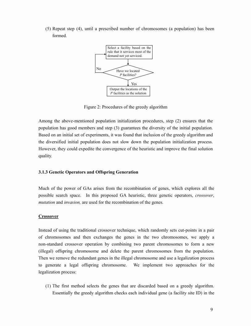
(1) Create a list of IDs for all eligible facility sites from 1 to J, each representing a gene. (2) Generate the first chromosome by selecting P facility sites based on a greedy algorithm,

as described in Figure 2. The greedy algorithm locates the facilities sequentially with an attempt to cover the most uncovered demand first. It terminates when all the P facilities have been located. Readers interested in the details of greedy algorithms for location problems are referred to Whitaker (1983) and Jain et al. (2002).

(3) Generate the next PJ / chromosomes by sequentially assigning different facilities to each chromosome. For example, the first chromosome is assigned with genes from 1 to P; the second chromosome assigned with genes from P+1 to 2P; and so on.

(4) Randomly select P facility sites to form the next chromosome;

9

(5) Repeat step (4), until a prescribed number of chromosomes (a population) has been formed.

Figure 2: Procedures of the greedy algorithm

Among the above-mentioned population initialization procedures, step (2) ensures that the population has good members and step (3) guarantees the diversity of the initial population. Based on an initial set of experiments, it was found that inclusion of the greedy algorithm and the diversified initial population does not slow down the population initialization process. However, they could expedite the convergence of the heuristic and improve the final solution quality.

3.1.3 Genetic Operators and Offspring Generation

Much of the power of GAs arises from the recombination of genes, which explores all the possible search space. In this proposed GA heuristic, three genetic operators, crossover, mutation and invasion, are used for the recombination of the genes.

Crossover

Instead of using the traditional crossover technique, which randomly sets cut-points in a pair of chromosomes and then exchanges the genes in the two chromosomes, we apply a non-standard crossover operation by combining two parent chromosomes to form a new (illegal) offspring chromosome and delete the parent chromosomes from the population. Then we remove the redundant genes in the illegal chromosome and use a legalization process to generate a legal offspring chromosome. We implement two approaches for the legalization process:

(1) The first method selects the genes that are discarded based on a greedy algorithm.

Essentially the greedy algorithm checks each individual gene (a facility site ID) in the

Select a facility based on the rule that it services most of the demand not yet serviced.

Have we located P facilities?

Output the locations of the P facilities as the solution

No

Yes

10

chromosome and removes the one that contributes the least to the improvement of the objective value in the location problem.

(2) The second method selects P genes to keep in the chromosome based on a small-scale GA. This GA selects P facilities from no more than 2P candidate facility sites that correspond to the genes in the illegal chromosomes. The steps of the small-scale GA follow the steps of a standard GA.

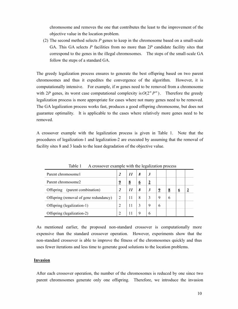
The greedy legalization process ensures to generate the best offspring based on two parent chromosomes and thus it expedites the convergence of the algorithm. However, it is computationally intensive. For example, if m genes need to be removed from a chromosome with 2P genes, its worst case computational complexity is )2( mm PO . Therefore the greedy legalization process is more appropriate for cases where not many genes need to be removed. The GA legalization process works fast, produces a good offspring chromosome, but does not guarantee optimality. It is applicable to the cases where relatively more genes need to be removed. A crossover example with the legalization process is given in Table 1. Note that the procedures of legalization-1 and legalization-2 are executed by assuming that the removal of facility sites 8 and 3 leads to the least degradation of the objective value.

Table 1 A crossover example with the legalization process

Parent chromosome1 2 11 8 3

Parent chromosome2 9 8 6 2

Offspring (parent combination) 2 11 8 3 9 8 6 2

Offspring (removal of gene redundancy) 2 11 8 3 9 6

Offspring (legalization-1) 2 11 3 9 6

Offspring (legalization-2) 2 11 9 6

As mentioned earlier, the proposed non-standard crossover is computationally more expensive than the standard crossover operation. However, experiments show that the non-standard crossover is able to improve the fitness of the chromosomes quickly and thus uses fewer iterations and less time to generate good solutions to the location problems.

Invasion After each crossover operation, the number of the chromosomes is reduced by one since two parent chromosomes generate only one offspring. Therefore, we introduce the invasion

11

operator. In an invasion operation, two new chromosomes are randomly generated. These two new chromosomes are compared with respect to their fitnesses, and the one with a larger fitness is added into the chromosome population. Then the remaining chromosome is compared with the worst chromosome in the current chromosome generation. If it is superior to the worst chromosome, it is added to the chromosome population to replace the worst chromosome. Otherwise, the worst chromosome is kept in the current population and the invading chromosome (the worse one of the two) is discarded. There are two advantages for applying the invasion operation. First, the search space can be extended and the genetic diversity of the chromosomes can be maintained. Second, the invasion of the new chromosomes and the survival of the better ones help to improve the average fitness of the chromosome population, which correspondingly, increases the possibility of finding the optimal or near optimal solution to the problem.

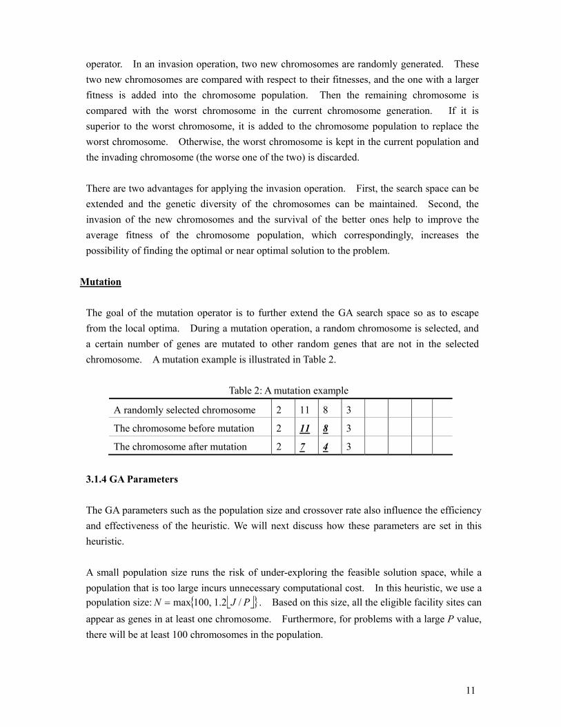
Mutation

The goal of the mutation operator is to further extend the GA search space so as to escape from the local optima. During a mutation operation, a random chromosome is selected, and a certain number of genes are mutated to other random genes that are not in the selected chromosome. A mutation example is illustrated in Table 2.

Table 2: A mutation example

A randomly selected chromosome 2 11 8 3

The chromosome before mutation 2 11 8 3

The chromosome after mutation 2 7 4 3 3.1.4 GA Parameters

The GA parameters such as the population size and crossover rate also influence the efficiency and effectiveness of the heuristic. We will next discuss how these parameters are set in this heuristic. A small population size runs the risk of under-exploring the feasible solution space, while a population that is too large incurs unnecessary computational cost. In this heuristic, we use a population size: { ,100max=N }PJ /2.1 . Based on this size, all the eligible facility sites can appear as genes in at least one chromosome. Furthermore, for problems with a large P value, there will be at least 100 chromosomes in the population.

12

The crossover rate determines that how many chromosomes in each iteration will be involved in the crossover operation. On an initial set of experiments, it was found that when the chromosome population size is equal to100, a 35 percent crossover rate enables the GA to generate good solutions in an efficient manner; while when the population size is more than 100, a 15 percent to 25 percent crossover rate is more appropriate. Furthermore, it was found that in general, inclusion of the mutation operation enables the GA to generate better solutions. However, different mutation rates seem not to have an obvious effect to the convergence speed. Therefore, we set the mutation rate to a relatively low value, 5 percent to 10 percent, in order to save computational time. During the crossover operation and mutation operation, different chromosome selection strategies such as linear ranking method (Ladd, 1996), roulette wheel method (Gen and Cheng, 2000), and random method have been experimented. It was found that different methods do not have distinct effects on the heuristic convergence, because although the linear ranking method and roulette wheel method have certain computational benefits (i.e. making the better chromosomes more likely to be selected in the next chromosome generation), the fitness sorting process in these methods consumes computational time and thus offsets the benefits. Therefore, we apply the random chromosome selection method in this heuristic.

3.1.5 GA Termination During each GA iteration, the best chromosome found so far is recorded. The heuristic terminates when any one of the following conditions is satisfied:

(1) A pre-specified number of iterations has been executed; (2) The best chromosome does not change within a pre-specified number of successive

iterations. (3) A full demand point coverage has been achieved.

Upon termination, the best chromosome is outputted as the solution to the location problem. 3.2 A Locate-Allocate Heuristic The locate-allocate (LocAlloc) heuristic was first proposed to solve traditional location problems by Cooper (1964), in which each demand point needs to be serviced by only a single (closest) facility. Since then it has become a widely used approach to solve different location problems (see for example, Larson and Brandeau, 1986; Taillard 2003). The LocAlloc heuristic uses the property that the separate phases (i.e. locating and allocating) of the location problems are each easy to solve, although the combined problem is difficult.

13

Compared with other algorithms for location problems (particularly the large-sized problems), the LocAlloc heuristic usually provides a good solution within a relatively short computational time. When applied to traditional location problems, the steps of the LocAlloc heuristic are:

(1) Choose an initial location for each of the P facilities; (2) Given the locations, find the best demand point allocation; (3) Given the allocation, divide the demand points into P groups (each centered by a

facility) and find the best facility location for each group; (4) If any of the locations has changed, repeat (2) and (3); otherwise stop.

When the LocAlloc heuristic is applied to solve the location problems with multiple facility quantity-of-coverage and quality-of-coverage requirements, two major problems occur. First, since each demand point is required to be serviced by multiple facilities at different quality levels, the demand points need to be allocated to more than one facility. Consequently each demand point may not belong to only one demand point group. Second, each facility services the demand points at different groups and hence the re-location of each facility needs to consider the demand points that need to be serviced at distinct quality levels. In what follows we propose an adapted LocAlloc heuristic. This heuristic follows the basic four steps of a standard LocAlloc heuristic. However, changes have been made in each step to enable the heuristic to deal with the location problems with multiple facility quantity-of-coverage and quality-of-coverage requirements. In this adapted LocAlloc heuristic, the initial solution plays a significant role in the algorithm convergence and the final solution quality. As such, the greedy algorithm described in Section 3.1.2 is applied to generate a good initial facility location solution. Then this initial solution is used for the allocation-location iteration for solution improvement. During each allocation-location iteration, the new generation of the P facility locations is compared with the pervious P facility locations. If there is any change in the facility location for any demand point group, the allocation-location iteration continues; otherwise, the iteration terminates and the result is outputted as the final location solution. 3.2.1 Allocation of the Demand Points After the initial locations of the P facilities have been determined, the demand points can be allocated to the facilities. We allow multiple allocation of a demand point to different

facilities. For each demand point i, it is allocated to the closest 1iQ facilities (a required

quantity of facilities at quality level 1), and then to the 2iQ facilities (a required quantity of

14

facilities at quality level 2, i.e. the first 1iQ facilities plus the 2

iQ - 1iQ facilities that are

farther than the first 1iQ facilities), and so on. As mentioned earlier, since there is no

precedence requirement in the covering provided for a given demand point, such a demand point allocation always leads to a feasible solution (also the best solution, given that the facility locations have been determined) to the problem. For each facility, we define all the demand points that have been allocated to it as a group. To differentiate the demand points that are serviced by the facility at different quality levels, a demand point group is further divided into a number of sub-groups. Sub-group 1 consists of the demand points that are serviced by the facility at the first quality level, and sub-group 2 consists of the demand points serviced at the second quality level, and so on. Figure 3 illustrates an example in which each demand point receives services from two facilities (one at quality level 1 and two at quality level 2) and therefore belongs to two demand point groups. For each group, the demand points can be further divided into sub-group 1 and sub-group 2, which include the demand points serviced by the facility at the first and second quality levels respectively.

Figure 3: Allocation of demand points to facilities

3.2.2 Relocation of Facilities After the demand point allocation, P demand point groups are obtained, each centered by a facility. In each group, the demand points are required to be serviced by the facility at different quality levels (i.e. sub-group1, sub-group2, etc.). With such a service arrangement in each demand point group, the selected facility is not necessarily the best one, and hence

Demand points

Facilities First quality coverage allocation Second quality coverage allocation

Sub-group1 that consists of demand points under first quality coverage

A demand point group

Sub-group2 that consists of demand points under second quality coverage

15

other unselected eligible facility sites need to be assessed. The best one can be determined by comparing the objective values of different facility location selections. It is important to note that when a facility location is evaluated, the objective value should be calculated by giving corresponding weights (as defined in the location models) to the demand points in different sub-groups. For example, if the location problem emphasizes the facilities that are closest to the demand points, then a larger weight should be assigned to the demand points that are in subgroup1, as opposed to the demand points at other subgroups ( qccc ≥≥≥ ...21 ). As such, for each demand point group, the objective value of a new facility location can be calculated as follows:

∑∑∈

=r Gi

iir

r

dMcvalueObjective_

where cr is the weight for sub-group r, Gr is the demand point set of subgroup r, and id is the distance from demand point i to the newly selected facility. To determine the best facility to service each demand point group, the eligible facility site that has a minimum objective value is selected as the new facility location for a demand point group. The re-location of the facilities and the allocation of the demand points to the facilities will be repeated. The heuristic terminates if in the re-location step, none of the locations of the selected facilities have changed. 3.3 A Lagrangean Relaxation Heuristic The GA heuristic and the LocAlloc heuristic have the potential to generate efficient solutions to the considered maximal covering problem. However, these heuristics do not provide information on how far the solutions are possibly away from optimality. In this section, we develop a Lagrangean relaxation (LR) heuristic, which, in addition to generating good solutions to the location problems, also provides bounds on the optimal objective value of the maximal covering location problem. The application of LR techniques to solve location covering problems is very limited in the literature. Pirkul and Schilling (1989) proposed a LR to solve a capacitated maximal covering location problem and presented extensive computational experiment results. Weaver and Church (1984) tested the performance of a LR in solving the covering location problem. However, in their research no conclusive results are reported. Galvão and ReVelle (1996) proposed a Lagrangean heuristic for the standard maximal covering location problem. The heuristic was tested in networks of up to 150 vertices and good performance of the heuristic in terms of the computational time and the final solution quality were obtained. Holmberg and Ling (1997) developed a Lagrangean heuristic, including Lagrangean relaxation and subgradient optimization, to solve the capacitated facility location

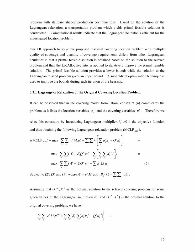
16

problem with staircase shaped production cost functions. Based on the solution of the Lagrangean relaxation, a transportation problem which yields primal feasible solutions is constructed. Computational results indicate that the Lagrangean heuristic is efficient for the investigated location problem. Our LR approach to solve the proposed maximal covering location problem with multiple quality-of-coverage and quantity-of-coverage requirements differs from other Lagrangean heuristics in that a primal feasible solution is obtained based on the solution to the relaxed problem and then the LocAlloc heuristic is applied to iteratively improve the primal feasible solution. The primal feasible solution provides a lower bound; while the solution to the Lagrangean relaxed problem gives an upper bound. A subgradient optimization technique is used to improve the bounds during each iteration of the heuristic. 3.3.1 Lagrangean Relaxation of the Original Covering Location Problem It can be observed that in the covering model formulation, constraint (4) complicates the

problem as it links the location variables jx and the covering variables riu . Therefore we

relax this constraint by introducing Lagrangean multipliers 0≥riλ in the objective function

and thus obtaining the following Lagrangean relaxation problem (MCLP 0≥λ ).

v(MCLP 0≥λ ) = max ∑ ∑∑∑∑

−+

i j

ri

rij

rij

r

ri

r

rii

r

iuQxauMc λ ≡

max jr j i r

ri

rij

i

ri

ri

ri

ri xauQA∑ ∑ ∑∑∑

+− λλ )( ≡

max jr j

ji

ri

ri

ri

ri xBuQA∑ ∑∑ +− )()( λλ (6)

Subject to (2), (3) and (5), where irr

i McA = and ∑∑=i r

ri

rijj aB λλ)( .

Assuming that ( ), LL XU is the optimal solution to the relaxed covering problem for some

given values of the Lagrangean multipliers riλ , and ( ** , XU ) is the optimal solution to the

original covering problem, we have

∑ ∑∑∑∑

−+

i j

Lri

ri

Lj

rij

r

ri

r

Lrii

r

iuQxauMc λ ≥

17

∑ ∑∑∑∑

−+

i j

ri

rij

rij

r

ri

r

rii

r

iuQxauMc ***

λ ≥ ∑∑r

rii

r

iuMc *

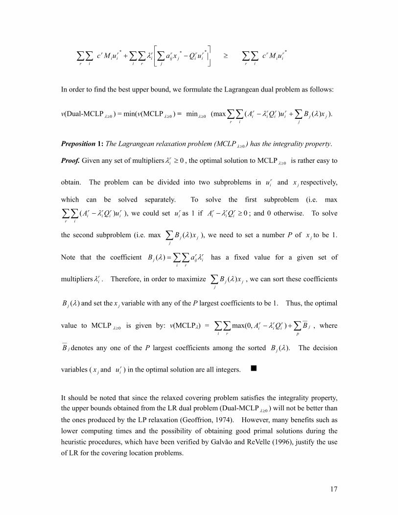
In order to find the best upper bound, we formulate the Lagrangean dual problem as follows:

v(Dual-MCLP 0≥λ ) = min(v(MCLP 0≥λ ) = 0min ≥λ (max jr j

ji

ri

ri

ri

ri xBuQA∑ ∑∑ +− )()( λλ ).

Preposition 1: The Lagrangean relaxation problem (MCLP 0≥λ ) has the integrality property.

Proof. Given any set of multipliers 0≥riλ , the optimal solution to MCLP 0≥λ is rather easy to

obtain. The problem can be divided into two subproblems in riu and jx respectively,

which can be solved separately. To solve the first subproblem (i.e. max

∑∑ −r i

ri

ri

ri

ri uQA )( λ ), we could set r

iu as 1 if 0≥− ri

ri

ri QA λ ; and 0 otherwise. To solve

the second subproblem (i.e. max ∑j

jj xB )(λ ), we need to set a number P of jx to be 1.

Note that the coefficient ∑∑=i r

ri

rijj aB λλ)( has a fixed value for a given set of

multipliers riλ . Therefore, in order to maximize ∑

jjj xB )(λ , we can sort these coefficients

)(λjB and set the jx variable with any of the P largest coefficients to be 1. Thus, the optimal

value to MCLP 0≥λ is given by: v(MCLPλ) = ∑ ∑∑ +−i p

jr

ri

ri

ri BQA ),0max( λ , where

jB denotes any one of the P largest coefficients among the sorted ).(λjB The decision

variables ( jx and riu ) in the optimal solution are all integers. g

It should be noted that since the relaxed covering problem satisfies the integrality property, the upper bounds obtained from the LR dual problem (Dual-MCLP 0≥λ ) will not be better than the ones produced by the LP relaxation (Geoffrion, 1974). However, many benefits such as lower computing times and the possibility of obtaining good primal solutions during the heuristic procedures, which have been verified by Galvão and ReVelle (1996), justify the use of LR for the covering location problems.

18

It has been shown that for any given set of multipliers 0≥riλ , the relaxed covering problem

can be readily solved to optimality and thus an upper bound to the original problem can be obtained. However, the solution to the relaxed problem is likely to violate constraint (4) in the original problem, thus being infeasible to the original covering problem. We find a primal feasible solution by the following feasibility procedure: we fix the location variables

jx in the solution to the relaxed problem and update the covering variables riu . Each

covering variable riu can be updated by checking if demand point i has been covered at

quality level r by the selected P facilities (determined by the location variables jx ). This

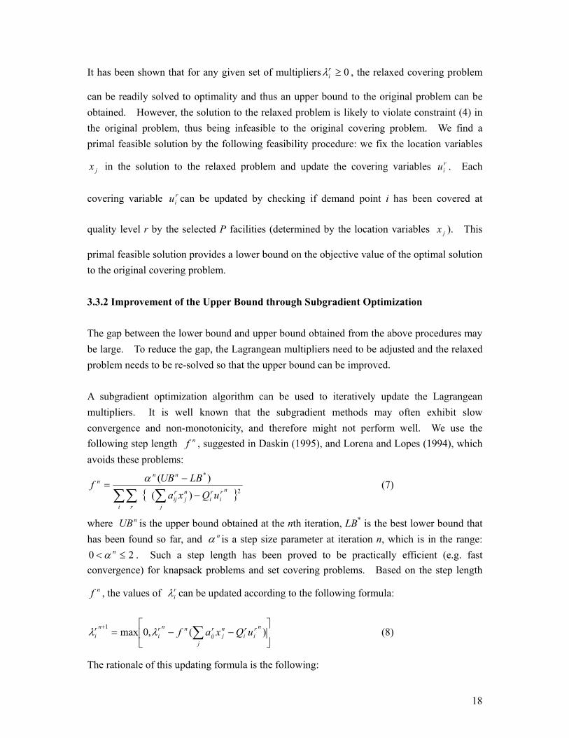
primal feasible solution provides a lower bound on the objective value of the optimal solution to the original covering problem. 3.3.2 Improvement of the Upper Bound through Subgradient Optimization The gap between the lower bound and upper bound obtained from the above procedures may be large. To reduce the gap, the Lagrangean multipliers need to be adjusted and the relaxed problem needs to be re-solved so that the upper bound can be improved. A subgradient optimization algorithm can be used to iteratively update the Lagrangean multipliers. It is well known that the subgradient methods may often exhibit slow convergence and non-monotonicity, and therefore might not perform well. We use the following step length nf , suggested in Daskin (1995), and Lorena and Lopes (1994), which avoids these problems:

{ }∑ ∑∑ −

−=

i j

nri

ri

nj

rij

r

nnn

uQxaLBUBf

2

*

)()(α (7)

where nUB is the upper bound obtained at the nth iteration, LB* is the best lower bound that has been found so far, and nα is a step size parameter at iteration n, which is in the range:

20 ≤< nα . Such a step length has been proved to be practically efficient (e.g. fast convergence) for knapsack problems and set covering problems. Based on the step length

nf , the values of riλ can be updated according to the following formula:

−−= ∑+

j

nri

ri

nj

rij

nnri

nri uQxaf )(,0max1

λλ (8)

The rationale of this updating formula is the following:

19

• If there are more than a required quantity of sites covering demand point i at quality

level r (i.e. ∑ >j

nri

ri

nj

rij uQxa ) , then the nr

iλ will be reduced to make it more likely

to have 11=

+nriu (because r

iri

ri QA λ− is increased) and less likely to select any

eligible facility site j to cover demand pint i (because ∑∑=i r

ri

rijj aB λ is reduced).

• On the other hand, if 1=nriu (i.e. 0≥− r

iri

ri QA λ ), but less than a required quantity

of facilities can cover demand point i at quality level r (i.e. ∑ <j

nri

ri

nj

rij uQxa ) , we

will have nri

nri λλ >

+1 . Since riλ is increased, it is less likely to have 1=r

iu in the

next iteration, but the likelihood for eligible site j to be selected to cover demand

point i ( )1=jx in the next iteration will be increased.

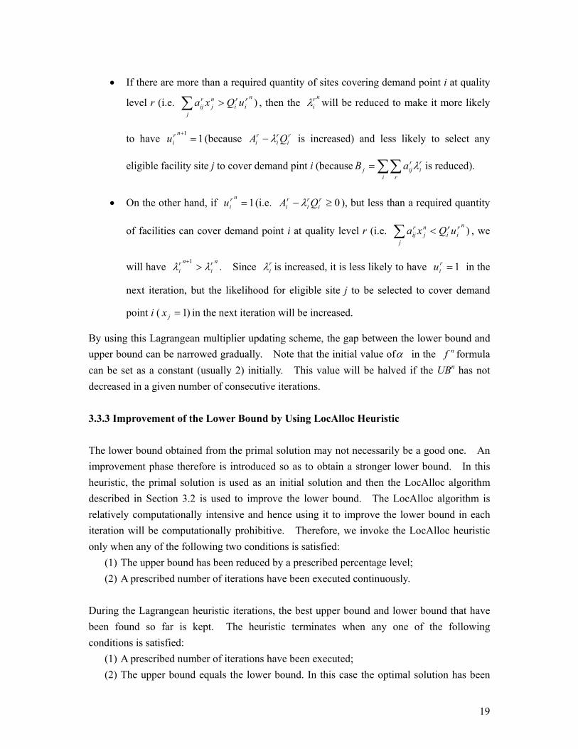
By using this Lagrangean multiplier updating scheme, the gap between the lower bound and upper bound can be narrowed gradually. Note that the initial value ofα in the nf formula can be set as a constant (usually 2) initially. This value will be halved if the UBn has not decreased in a given number of consecutive iterations. 3.3.3 Improvement of the Lower Bound by Using LocAlloc Heuristic The lower bound obtained from the primal solution may not necessarily be a good one. An improvement phase therefore is introduced so as to obtain a stronger lower bound. In this heuristic, the primal solution is used as an initial solution and then the LocAlloc algorithm described in Section 3.2 is used to improve the lower bound. The LocAlloc algorithm is relatively computationally intensive and hence using it to improve the lower bound in each iteration will be computationally prohibitive. Therefore, we invoke the LocAlloc heuristic only when any of the following two conditions is satisfied:

(1) The upper bound has been reduced by a prescribed percentage level; (2) A prescribed number of iterations have been executed continuously.

During the Lagrangean heuristic iterations, the best upper bound and lower bound that have been found so far is kept. The heuristic terminates when any one of the following conditions is satisfied:

(1) A prescribed number of iterations have been executed; (2) The upper bound equals the lower bound. In this case the optimal solution has been

20

found; (3) The total demand point coverage has been achieved in the primal solution. The

optimal solution has been found; (4) The value of the parameter nf is less than 0.01; In this case, a duality gap exists and

the best solution is given by the best lower bound. The steps of the complete LR heuristic is described in detail in the Appendix. 4. Illustrative Examples and Performance Analyses

In this section we benchmark the three heuristics presented in the pervious sections and compare their computational performance on illustrative facility location examples for large-scale emergencies. The emergency instance we consider is an anthrax emergency in Los Angeles County, which has a total population of 9.5 million. Anthrax is an acute infectious disease caused by the spore-forming bacterium. There are several types of anthrax infections (cutaneous, inhalation, and gastrointestinal) and each requires vaccines and antibiotics to cure the infected people and immunize the high-risk population. During an anthrax emergency, the strategic national stockpiles (SNS) are mobilized for local emergency medical services. The problem is then to select a given number of eligible facility sites as staging areas for mass distribution of the medical supplies from the SNS to cover as much of the population as possible. To formulate the facility location problem, we first identify the demand points. We use the population density pattern that is available for Los Angeles County (ESRI website, 2005), and consider the centroid of each census tract as a demand point to represent the aggregated population in this tract. Thus we obtain 2054 discrete demand points that have different population densities. In addition, we select the set of eligible facility sites by deviating the facility sites that were identified by the emergency management of Los Angeles County by a small distance. The county has identified a little over 200 eligible facility sites. In this paper, we use 200 as the number of eligible facility sites. Figure 4 depicts the distribution of the 2054 demand points in Los Angeles County (for confidentiality, the detailed number of the facility sites and the distribution of the eligible facility sites are not depicted in the figure). To ensure adequate facility service, we consider multiple quantity coverage requirements for the demand points. The quantity requirements for a single quality level are dependent on the population at each demand point and they are defined as follows:

(1) Qi = 1, if the population of demand point i is less than 3000;

21

(2) Qi = 2, if the population of demand point i is between 3000 and 6000; (3) Qi = 3, if the population of demand point i is between 6000 and 9000; (4) Qi = 4; if the population of demand point i is greater than 9000.

Furthermore, we use double-quality-coverage to provide medical services for each demand point. The distance requirements for the first and second quality levels are defined respectively as 8 km and 16 km. We consider the quantity of facilities required to service a demand point at the second quality level double the quantity of facilities required at the first quality level. For example, if a demand point has a population of 5392, then two facilities will be required at quality level 1 (within 8 km of the demand point), and 4 facilities will be required at quality level 2 (within 16 km of the demand point). In addition, for simplicity, we define the two different quality level coverages have the same importance, i.e. c1 = c2.

Figure 4. Demand point distribution in Los Angeles County In this section we present two groups of experiments, which are: (1) benchmark the three heuristics by solving different problem instances, and (2) investigate the best way of opening facilities in a sequential manner. These experiments were conducted on a Dell Inspiron computer with a Pentium M chip running at 1.73MHz using 512 MB of memory ram. 4.1 Performance Comparison of the Three Heuristics In this section, we compare the computational performance of the three heuristics. We formulate a series of location problems by sequentially setting the number of selected facilities (i.e. the value of parameter P) as 10, 15, 20, 30, 40, 50, 60, 70, and 80. We first use the three heuristics to solve each of the problem instances. Furthermore, to evaluate the quality of the solutions obtained from the heuristics, we also use CPLEX, a commercially available software package, to solve the location problems. The time limit set for CPLEX is

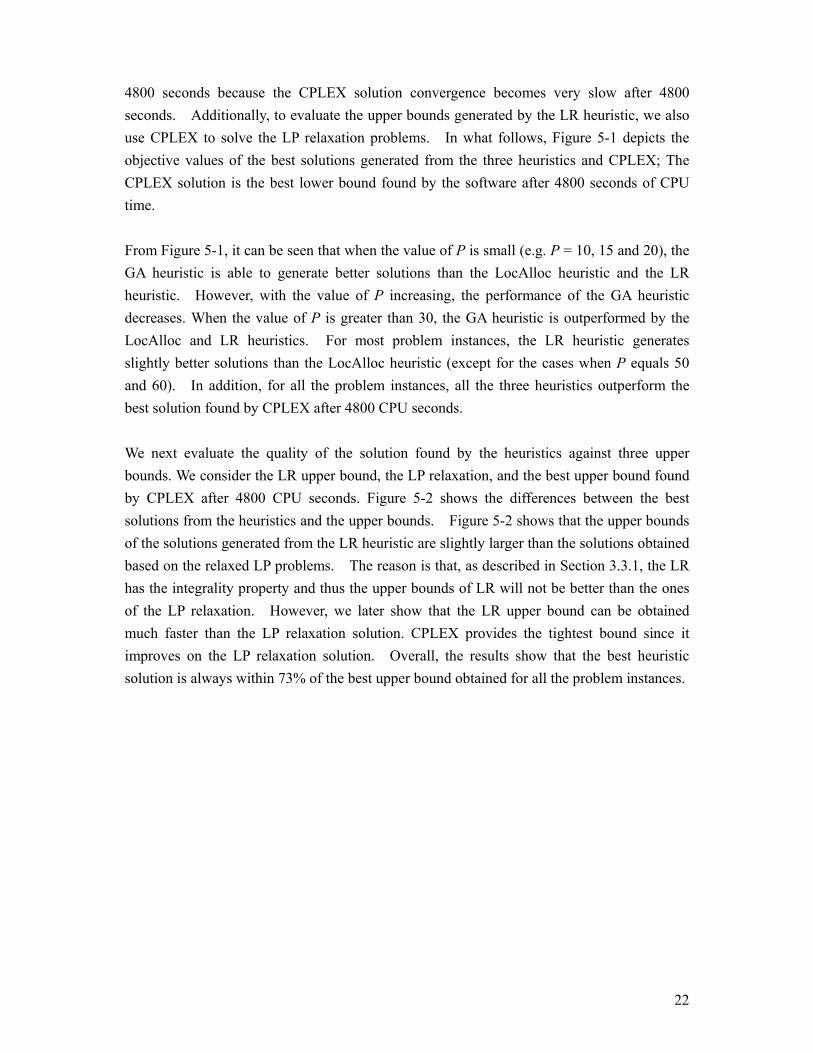
22

4800 seconds because the CPLEX solution convergence becomes very slow after 4800 seconds. Additionally, to evaluate the upper bounds generated by the LR heuristic, we also use CPLEX to solve the LP relaxation problems. In what follows, Figure 5-1 depicts the objective values of the best solutions generated from the three heuristics and CPLEX; The CPLEX solution is the best lower bound found by the software after 4800 seconds of CPU time. From Figure 5-1, it can be seen that when the value of P is small (e.g. P = 10, 15 and 20), the GA heuristic is able to generate better solutions than the LocAlloc heuristic and the LR heuristic. However, with the value of P increasing, the performance of the GA heuristic decreases. When the value of P is greater than 30, the GA heuristic is outperformed by the LocAlloc and LR heuristics. For most problem instances, the LR heuristic generates slightly better solutions than the LocAlloc heuristic (except for the cases when P equals 50 and 60). In addition, for all the problem instances, all the three heuristics outperform the best solution found by CPLEX after 4800 CPU seconds.

We next evaluate the quality of the solution found by the heuristics against three upper bounds. We consider the LR upper bound, the LP relaxation, and the best upper bound found by CPLEX after 4800 CPU seconds. Figure 5-2 shows the differences between the best solutions from the heuristics and the upper bounds. Figure 5-2 shows that the upper bounds of the solutions generated from the LR heuristic are slightly larger than the solutions obtained based on the relaxed LP problems. The reason is that, as described in Section 3.3.1, the LR has the integrality property and thus the upper bounds of LR will not be better than the ones of the LP relaxation. However, we later show that the LR upper bound can be obtained much faster than the LP relaxation solution. CPLEX provides the tightest bound since it improves on the LP relaxation solution. Overall, the results show that the best heuristic solution is always within 73% of the best upper bound obtained for all the problem instances.

23

2

3

4

5

6

7

8

9

10 15 20 30 40 50 60 70 80P-Value

Obj

ectiv

e Va

lue

GA

LR

LocAlloc

CPLEX-LB

Figure 5-1: Objective values of the best solutions

2

4

6

8

10

12

14

16

18

10 15 20 30 40 50 60 70 80P-Value

Obj

ectiv

e Va

lue

CPLEX-UB

LR-UB

LP-Relaxation

Heuristic (Best)

Figure 5-2: Comparison of the best heuristic solutions and the upper bounds

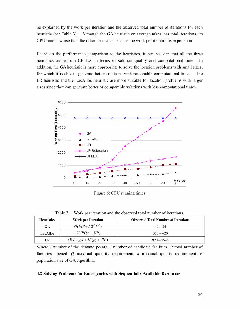
To evaluate the convergence performance of the heuristics, we also compare the computational time for the heuristics to solve each problem instance, as depicted in Figure 6. From this figure, it can be seen that the LocAlloc heuristic always uses the least amount of computational time to generate the solutions for all the problems. The CPU time of the GA heuristic increases rapidly as the problem size increases. The computation time of the LR heuristic is higher than that for LocAlloc. In addition, the LR heuristic uses less time to solve the problems and generate the bounds than the LP relaxation does. Such running times can

24

be explained by the work per iteration and the observed total number of iterations for each heuristic (see Table 3). Although the GA heuristic on average takes less total iterations, its CPU time is worse than the other heuristics because the work per iteration is exponential. Based on the performance comparison to the heuristics, it can be seen that all the three heuristics outperform CPLEX in terms of solution quality and computational time. In addition, the GA heuristic is more appropriate to solve the location problems with small sizes, for which it is able to generate better solutions with reasonable computational times. The LR heuristic and the LocAlloc heuristic are more suitable for location problems with larger sizes since they can generate better or comparable solutions with less computational times.

0

1000

2000

3000

4000

5000

6000

10 15 20 30 40 50 60 70 80P-Value

Run

ning

Tim

e (S

econ

ds) .

GA

LocAlloc

LR

LP-Relaxation

CPLEX

Figure 6: CPU running times

Table 3. Work per iteration and the observed total number of iterations.

Heuristics Work per Iteration Observed Total Number of Iterations

GA )2( PP PFFIPO + 46 – 84

LocAlloc )( JIPIPQqO + 320 – 620

LR )log( JIPIPQqJJO ++ 920 – 2540

Where I number of the demand points, J number of candidate facilities, P total number of facilities opened, Q maximal quantity requirement, q maximal quality requirement, F population size of GA algorithm.

4.2 Solving Problems for Emergencies with Sequentially Available Resources

25

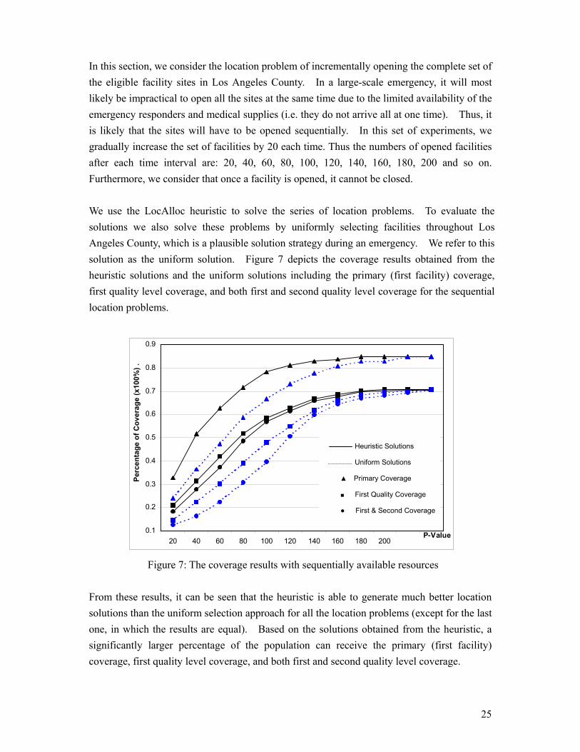
In this section, we consider the location problem of incrementally opening the complete set of the eligible facility sites in Los Angeles County. In a large-scale emergency, it will most likely be impractical to open all the sites at the same time due to the limited availability of the emergency responders and medical supplies (i.e. they do not arrive all at one time). Thus, it is likely that the sites will have to be opened sequentially. In this set of experiments, we gradually increase the set of facilities by 20 each time. Thus the numbers of opened facilities after each time interval are: 20, 40, 60, 80, 100, 120, 140, 160, 180, 200 and so on. Furthermore, we consider that once a facility is opened, it cannot be closed. We use the LocAlloc heuristic to solve the series of location problems. To evaluate the solutions we also solve these problems by uniformly selecting facilities throughout Los Angeles County, which is a plausible solution strategy during an emergency. We refer to this solution as the uniform solution. Figure 7 depicts the coverage results obtained from the heuristic solutions and the uniform solutions including the primary (first facility) coverage, first quality level coverage, and both first and second quality level coverage for the sequential location problems.

0.1

0.2

0.3

0.4

0.5

0.6

0.7

0.8

0.9

20 40 60 80 100 120 140 160 180 200P-Value

Perc

enta

ge o

f Cov

erag

e (x

100%

) .

Figure 7: The coverage results with sequentially available resources

From these results, it can be seen that the heuristic is able to generate much better location solutions than the uniform selection approach for all the location problems (except for the last one, in which the results are equal). Based on the solutions obtained from the heuristic, a significantly larger percentage of the population can receive the primary (first facility) coverage, first quality level coverage, and both first and second quality level coverage.

Heuristic Solutions

Uniform Solutions

▲ Primary Coverage

■ First Quality Coverage

● First & Second Coverage

26

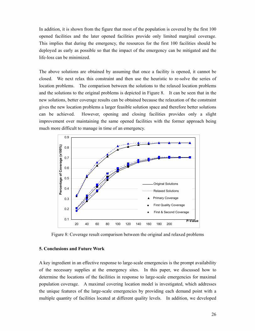
In addition, it is shown from the figure that most of the population is covered by the first 100 opened facilities and the later opened facilities provide only limited marginal coverage. This implies that during the emergency, the resources for the first 100 facilities should be deployed as early as possible so that the impact of the emergency can be mitigated and the life-loss can be minimized. The above solutions are obtained by assuming that once a facility is opened, it cannot be closed. We next relax this constraint and then use the heuristic to re-solve the series of location problems. The comparison between the solutions to the relaxed location problems and the solutions to the original problems is depicted in Figure 8. It can be seen that in the new solutions, better coverage results can be obtained because the relaxation of the constraint gives the new location problems a larger feasible solution space and therefore better solutions can be achieved. However, opening and closing facilities provides only a slight improvement over maintaining the same opened facilities with the former approach being much more difficult to manage in time of an emergency.

0.1

0.2

0.3

0.4

0.5

0.6

0.7

0.8

0.9

20 40 60 80 100 120 140 160 180 200P-Value

Perc

enta

ge o

f Cov

erag

e (x

100%

)

Figure 8: Coverage result comparison between the original and relaxed problems

5. Conclusions and Future Work A key ingredient in an effective response to large-scale emergencies is the prompt availability of the necessary supplies at the emergency sites. In this paper, we discussed how to determine the locations of the facilities in response to large-scale emergencies for maximal population coverage. A maximal covering location model is investigated, which addresses the unique features of the large-scale emergencies by providing each demand point with a multiple quantity of facilities located at different quality levels. In addition, we developed

Original Solutions

Relaxed Solutions

▲ Primary Coverage

■ First Quality Coverage

● First & Second Coverage

27

three heuristics to solve the maximal covering problem in an efficient manner. The studied models and developed heuristics have been tested by using an anthrax emergency example in the Los Angeles County area. The results imply a good capability of the model in improving the population coverage and reducing life-loss during large-scale emergencies. Additionally, the computational performance of the three heuristics in solving different problem instances is evaluated and suggestions have been given in selecting the appropriate heuristic for different problem instances. Finally we studied the sequence in which facilities should be opened in response to a large-scale emergency. The examples have shown that the heuristics are able to generate facility location solutions in an efficient and effective manner. In comparison, the GA heuristic is more appropriate to solve the location problems with small sizes, for which it is able to generate better solutions with reasonable computational times; The LR heuristic and the LocAlloc heuristic are more suitable for location problems with larger sizes since they can generate better or comparable solutions with less computational times. The maximal covering model studied in this paper is suitable for certain types of large-scale emergencies. However it may not be appropriate for all types of emergencies. For example, for emergencies in which all demand points in an area need to be simultaneously serviced or the worst case performance of the facilities needs to be avoided, the P-median or P-center model may be more appropriate to use. Detailed descriptions of different types of large-scale emergencies and discussions of the applicability of different location models to various large-scale emergencies can be found in Jia et al. (2005). Although the heuristics in this paper are developed to solve the maximal covering problems, they may be adapted to solve the P-median problems and P-center problems with multiple quantity and quality coverage requirement as well. For example, the GA heuristic can tackle the P-median and P-center problems with modifications only in the chromosome fitness evaluation step, based on the corresponding objective functions of the P-median and P-center models. Our future research direction will focus on developing the modified heuristics and then using them to test different P-median and P-center problems for other types of large-scale emergencies.

28

Appendix The complete steps of the LR heuristic is as follows:

1. Problem

Initialization

(a) Read all the data related to the demand points and eligible facility sites;

(b) Initialize the lagrangean multipliers riλ ;

(c) Compute parameters ,, rij

ri aA and jB ;

(d) Set initial UB = ∞+ , LB = ∞− , and 2=α ;

(e) Set UB_counter, Alaph_counter, Iter_counter = 0; These counters are used to

determine the execution of the LocAlloc heuristic, the update of the parameter of

α , and the total number of iterations of the heuristic.

2. Solve Relaxed

Covering Problem

(a) Solve the relaxed covering problem (6), described in section 3.3.1, to obtain the

optimal solution to the relaxed problem;

(b) Using the feasibility procedure in section 3.3.1, obtain a primal solution;

(c) Calculate the new UB and LB for the current iteration;

(d) Set Iter_counter = Iter_counter +1.

3. Bounds Update (a) If the new UB obtained in step 2 is better than the UB found so far, update the UB

and reset Alaph_counter = 0.

(a-1) If the UB improvement is greater than the prescribed percentage level, apply

the LocAlloc heuristic to update the primal solution and lower bound. Reset

UB_counter = 0;

(a-2) If the improvement is less than the prescribed percentage, set UB_counter =

UB_counter +1.

(b) If the new UB obtained in step 2 is not better than the UB found so far, ignore the

new UB. Set UB_counter = UB_counter +1, and Alaph_counter =

Alaph_counter+1;

(c) If UB_counter is greater than a prescribed value, execute the LocAlloc heuristic to

update the primal solution and lower bound. Reset UB_counter = 0;

4.Update Parameter α (a) If Alaph_counter is greater than the prescribed value, set α =α /2.

5. Update Lagrangean

Multipliers riλ

(a) Calculate parameter nf using (7) and update the Lagrangean multipliers riλ using

(8).

29

6. Check the Heuristic

Termination

Conditions

(a) If any one of the following conditions is satisfied, stop the heuristic and output the

bounds and solutions to the problems; (a-1) Iter_counter has reached the prescribed value;

(a-2) The UB equals The LB; The optimal solution has been found;

(a-3) The value of the parameter nf is less than 0.01; A duality gap exists;

(a-4) The total demand point coverage has been achieved. The optimal solution

has been found.

(b) If none of the termination condition is satisfied, go to step 2 and continue the

heuristic.

References Aickelin, U. (2002). An indirect genetic algorithm for set covering problems. Journal of the

Operational Research Society, 53, pp. 1118-1126. Alp, O., Drezner, Z. and Erkut, E. (2003). An Efficient Genetic Algorithm for the p-Median

Problem. Annals of Operations Research, 122, pp.21-42. Al-Sultan, K. S. and Al-Fawzan, M. A. (1999). A tabu search approach to the uncapacitated

facility location problem. Annals of Operations Research, 86, pp.91–103. Alves, M. L. and Almeida M. T. (1992). Simulated annealing algorithm for the simple plant

location problem: A computational study. Revista Investigaćão Operacional, 12. Beasley, J.E and Chu, P.C. (1996). A genetic algorithm for the set covering problem.

European Journal of Operational Research, 94, pp. 392-404. Chen, B. and Lin, C.S. (1998). Minmax-regret robust 1-median location on a tree. Networks

31, pp. 93–103. Church, R. and ReVelle, C. (1974). The maximal covering location problem. Papers of the

Regional Science Association, 32, pp. 101-118. Cooper, L. (1964). Heuristic methods for location - allocation Problems. SIAM Review, 6, pp.

37-53. Daskin, M. S. (1995). Network and discrete location: models, algorithms, and applications.

30

John Wiley & Sons, New York. Dessouky, M. M., Ordóñez, F., Jia, H.Z. and Shen, Z.H. (2006). Rapid Distribution of

Medical Supplies, In: Delay Management in Health Care Systems, Hall, R. (ed), Springer, 2006.

Galvão, R.D. and ReVelle, C. (1996). A lagrangean heuristic for the maximal covering

location problem. European Journal of Operational Research, 88, pp.114-123. Gen, M. and Cheng, R. (2000). Genetic algorithms and engineering optimization. Wiley, New

York. Geoffrion, A.M. (1974). Lagrangean relaxation for integer programming, Mathematical

Programming Study, 2, pp. 82-114. Goldberg, D. E. (1989). Genetic algorithms in search, optimization and machine learning.

Reading, MA: Addison-Wesley. Hakimi, S.L. (1990). Locations with spatial interaction: competitive locations and games. In:

Mirchandani, P.B. and Francis, R.L. (ed.), Discrete Location Theory. New York: Wiley. Hogan, K. and ReVelle, C. (1986). Concepts and applications of backup coverage.

Management Science, 32, pp.1434-1444. Holmberg, K. and Ling, J. (1997). A lagrangean heuristic for the facility location problem

with staircase costs. European Journal of Operational Research, 97, pp. 63-74. Jacobsen, S.K. (1983). Heuristics for the capacitated plant location model. European Journal

of Operational Research, 12, pp.253-261. Jain, K., Mahdian, M. and Saberi, A. (2002). A new greedy approach for facility location

problems. Proceedings of the 34th Annual ACM symposium on Theory of Computing, pp. 731 – 740.

Jaramillo, J.H., Bhadury, J. and Batta, R. (2002). On the use of genetic algorithms to solve

location problems. Location Analysis, 29(6), pp. 761-779. Jia, H. Z., Ordóñez, F. and Dessouky, M. M. (2005). A modeling framework for facility

location of medical services for large-scale emergencies. USC-ISE Working paper

31

#2005-01. To appear in IIE Transactions. Kariv, O. and Hakimi, S. (1979). An algorithm approach to network location problem.

SIAM Journal of Applied Mathematics, 37, pp. 513-560. Larson, R.C. and Brandeau, M. (1986). Extending and applying the hypercube queueing

model to deploy ambulances in Boston. In: Swersey, A. and Ignall, E. (ed.), Delivery of Urban Services. New York: North Holland.

Ladd, S. R. (1996). Genetic algorithms in C++, M & T Books, New York. Lorena, L. and deSouza-Lopez L. (1977). GAs applied to computationally difficult set

covering problems. Journal of the Operational Research Society, 48, pp. 440-445. Lorena, L. and Lopes, F. (1994). A surrogate heuristic for set covering problems. European

Journal of Operational Research, 79, pp.138-50. Lorena, L. and Plateau, G. (1988). A monotone decreasing algorithm for the 0-1

multiknapsack dual problem. Research Report, 89-1, Université of Paris-Nord, France. Marianov, V. and ReVelle, C. (1996). The queueing maximal availability location problem: A

model for the siting of emergency vehicles. European Journal of Operational Research, 93, pp.110-120.

Megiddo, N., Zemel, E., and Hakimi, S.L. (1983). The maximum coverage location problem.

SIAM Journal of Algebraic and Discrete Methods, 4, pp. 253-261. Owen, S.H. and Daskin, M.S. (1998). Strategic facility location via evolutionary

programming. Working paper, Dept of Industrial Engineering and Management Science, Northwestern University, Evanston, Illinois.

Paluzzi, M. (2004). Testing a heuristic P-median location allocation model for siting

emergency service facilities. Paper Presented at the Annual Meeting of Association of American Geographers, Philadelphia, PA.

Pirkul, H. and Schilling, D (1989). The capacitated maximal covering location problem with

backup service. Annal of Operations Research, 18, pp. 141-154. Reeves, C.R. (1993). Modern heuristic techniques for combinatorial problems. John Wiley &

32

Sons, New York.

Schilling, D., Elzinga, D., Cohon, J., Church, R. and ReVelle, C. (1979). The TEAM/FLEET

models for simultaneous facility and equipment siting. Transportation Science, 13, pp. 163-175.

Snyder, L. V. (2006). Facility location under uncertainty: A review. To appear in IIE

Transactions. Snyder, L. V., and Daskin, M. S. (2006). Stochastic p-robust location problems. To appear

in IIE Transactions. Taillard, E.D. (2003). Heuristic methods for large centroid clustering problems. Journal of

Heuristics, 9, pp. 51-73. Toregas, C., Swain, R., ReVelle, C. and Bergman, L. (1971). The location of emergency

service facility. Operations Research, 19, pp. 1363-1373. Weaver, J.R., and Church, R.L. (1984). A comparison of direct and indirect primal

heuristic/dual bounding solution procedures for the maximal covering location problem. Working Paper.

Whitaker, R. (1983). A fast algorithm for the greedy interchange of large-scale clustering and

median location problems. INFOR, 21, pp. 95-108. CDC website (2005). http://www.cdc.gov/ ESRI website (2006). http://reports.esribis.com/