solar power for deployment in populated areas

Solar Power for

Deployment in Populated Areas

A Thesis

presented to

the Faculty of California Polytechnic State University

San Luis Obispo, California

In Partial Fulfillment

of the Requirements for the Degree

Master of Science in Architecture with a Specialization in Architectural Engineering

by

Nathan Hicks

June 2009

ii

© 2009

Nathan Hicks ALL RIGHTS RESERVED

iii

COMMITTEE MEMBERSHIP

TITLE: Solar Power for Deployment in Populated Areas

AUTHOR: Nathan Hicks

DATE SUBMITTED: June 2009

COMMITTEE CHAIR: Craig Baltimore, Ph.D., S.E.

COMMITTEE MEMBER: Kevin Dong, S.E.

COMMITTEE MEMBER: Ansgar Neuenhofer, Ph.D., P.E.

iv

ABSTRACT

Solar Power for Deployment in Populated Areas

Nathan Hicks

The thesis presents background on solar thermal energy and addresses the

structural challenges associated with the deployment of concentrating solar power fields

in urban areas. Two potential structural systems and urban locales of deployment are

proposed and investigated to determine whether they have the potential to be a cost-

effective renewable energy solution for urban areas. The structural issues explored in the

thesis include flutter, the wind loading of open frame structures, performance-based

design, and the design of flexibly mounted equipment on a building.

v

TABLE OF CONTENTS

List of Tables .................................................................................................................... vii

List of Figures .................................................................................................................. viii

List of Nomenclature .......................................................................................................... x

1.0 Purpose.................................................................................................................... 1

2.0 Introduction............................................................................................................. 2

2.1 Focus of the Thesis ............................................................................................. 2

2.2 Focus of the Overall Project ............................................................................... 4

2.3 Relevance of Research........................................................................................ 5

3.0 Background............................................................................................................. 7

3.1 Early Solar Thermal Energy Systems ................................................................. 8

3.2 Contemporary Solar Thermal Energy Systems................................................. 10

3.2.1 Solar Power Towers.................................................................................. 10

3.2.2 Solar Troughs............................................................................................ 12

3.2.3 Concentrating Photovoltaics and Thermal (CPVT).................................. 14

4.0 Research................................................................................................................ 17

4.1 Flutter................................................................................................................ 17

4.1.1 Reason for Investigation ........................................................................... 17

4.1.2 Early Investigation of Flutter .................................................................... 18

4.1.3 Current Investigation of Flutter ................................................................ 20

4.1.4 Conclusion on Flutter................................................................................ 22

vi

4.2 Wind Loading of Open Frame Structures......................................................... 22


4.2.2 Current Investigation of Wind Loading.................................................... 24

4.2.3 Conclusion on Wind Loading ................................................................... 30

4.3 Performance-Based Design............................................................................... 30


4.3.2 Early Investigation of Performance-Based Design................................... 32

4.3.3 Current Investigation of Performance-Based Design ............................... 36

4.3.4 Performance-Based Design Case Study.................................................... 39

4.3.5 Conclusion on Performance-Based Design .............................................. 59

5.0 Conclusion ............................................................................................................ 60

6.0 Glossary ................................................................................................................ 61

7.0 Acronyms.............................................................................................................. 64

8.0 References............................................................................................................. 65

9.0 Works Consulted................................................................................................... 67

vii

LIST OF TABLES

Table A – Damage vs. Building Performance Level ........................................................ 33

Table B – Earthquake Hazard Levels ............................................................................... 34

Table C – Building Performance Objectives .................................................................... 35

Table D – Mass Assignment ............................................................................................. 42

Table E – Mode Periods.................................................................................................... 42

Table F – Amplitude of Modal Displacements................................................................. 46

Table G – Modal Participation Factors............................................................................. 47

Table H – Values of Exponent n....................................................................................... 50

Table I – Modal Spectral Accelerations............................................................................ 53

Table J – Modal Story Acceleration ................................................................................. 54

Table K – First Mode Spectral Roof Response Acceleration Tabulation......................... 55

viii

LIST OF FIGURES

Figure A – CSP Field over Urban Parking Lot................................................................... 3

Figure B – CSP Field on Urban Industrial Building........................................................... 4

Figure C – Worldwide Energy Consumption ..................................................................... 5

Figure D – Solar Thermal Energy....................................................................................... 7

Figure E – Pifre’s Solar Concentrator................................................................................. 9

Figure F – Seville Solar Power Tower.............................................................................. 11

Figure G – Ivanpah Solar Power Tower ........................................................................... 11

Figure H – Solar Trough................................................................................................... 13

Figure I – Concentrating Photovoltaics ............................................................................ 15

Figure J – Brighton Chain Pier ......................................................................................... 19

Figure K – B/D Ratio Comparison ................................................................................... 21

Figure L – Heaving and Torsional Motion ....................................................................... 22

Figure M – Basic Wind Speed .......................................................................................... 24

Figure N – Wind Direction ............................................................................................... 25

Figure O – Plan View of Framing..................................................................................... 27

Figure P – Force Coefficient............................................................................................. 29

Figure Q – Performance-Based Design Flow Diagram .................................................... 36

Figure R – Response of Flexibly Mounted Equipment .................................................... 38

Figure S – Industrial Building Plan .................................................................................. 40

Figure T – ETABS Model................................................................................................. 41

ix

Figure U – Mode Shapes................................................................................................... 45

Figure V – USGS Ground Motion Calculator .................................................................. 48

Figure W – Design Response Spectrum at Ground Level ................................................ 51

Figure X – Design Magnification Factor vs. Period Ratio ............................................... 55

Figure Y – Roof Response Spectrum (EQ-1) ................................................................... 57

Figure Z – Roof Response Spectrum (EQ-2).................................................................... 58

x

LIST OF NOMENCLATURE

axm – Modal story acceleration at level x for mode m (g)

As – The gross area of the solid wall as defined in ASCE 7-05

Ag – The gross area of the wall including all openings as defined in ASCE 7-05

B – Frame width, measured from outside edge to outside edge

CDg – Force coefficient on the gross area of the wall

Cf – Force coefficient as defined in ASCE 7-05

Cs – Seismic response coefficient as defined in ASCE 7-05 (g)

Fp – Design force applied to solar tower (force)

G – Gust Factor as defined in ASCE 7-05

I – Importance Factor as defined in ASCE 7-05

Kzt – Wind topographic factor as defined in ASCE 7-05

N – Number of framing lines normal to the nominal wind direction

ps – Net design wind pressure as defined in ASCE 7-05 (lb/ft2)

pS30 – Simplified design wind pressure as defined in ASCE 7-05 (lb/ft2)

PEY – Probability of exceedance (expressed as a decimal) in time Y (years) for the desired

earthquake hazard level

PR – Return period of seismic event (year)

PFxm – Modal Participation Factor at level x for mode m

Sam – Spectral roof response acceleration of mode m

SDS – Design spectral response acceleration response parameter, 5 percent damped, at

short periods as defined in ASCE 7-05 (g)

xi

SD1 – Design spectral response acceleration response parameter, 5 percent damped, at a

period of 1 second as defined in ASCE 7-05 (g)

SMS – The MCE spectral response acceleration response parameter, 5 percent damped, at

short periods adjusted for site class effects as defined in ASCE 7-05 (g)

SM1 – The MCE spectral response acceleration response parameter, 5 percent damped, at

a period of 1 second adjusted for site class effects as defined in ASCE 7-05 (g)

SF – Frame spacing, measured from centerline to centerline

Sfa – Spectral roof response acceleration (g)

Ta – Period of solar power tower or other flexibly mounted equipment (sec)

Tm – Building period for mode m (sec)

TO – .2 SD1/SDS as defined in ASCE 7-05 (sec)

TS – SD1/SDS as defined in ASCE 7-05 (sec)

V – Seismic base shear as defined in ASCE 7-05 (force)

wi/g – Mass assigned at level I (k-sec2/ft)

W – Effective seismic weight as defined in ASCE 7-05 (force/g)

Wp – Effective seismic weight of the solar tower (force/g)

Y – Years for the desired earthquake hazard level (years)

α – Wind angle of attack

Φim – Amplitude of mode m at level I (dimensionless)

ε – Solidity ratio (As/Ag)

λ – Wind adjustment factor for building height and exposure as defined in ASCE 7-05

1.0 Purpose 1


1.0 PURPOSE

The purpose of the thesis is to present a single document exploring the structural

challenges and issues that arise when integrating solar thermal energy (STE) in an

urban environment through the use of concentrating solar power (CSP) fields. To

facilitate the purpose, the thesis has been organized into the following sections:

• The Introduction provides a synopsis of both the thesis and the overall project.

• The Background discusses solar thermal energy and the concentrating solar power

systems that have the potential to be deployed in urban areas.

• The Research reveals the key structural issues investigated in relation to the

deployment of concentrating solar power systems in urban areas.

Many terms related to alternative energy methods may be unfamiliar to

individuals outside of the field. As a result, a Glossary section (6.0) has been provided for

all bold words within the body of this thesis.

2.0 Introduction 2


2.0 INTRODUCTION

The objective of the thesis is to explore the deployment of concentrating solar

power (CSP) fields in urban areas in order to provide solar thermal energy (STE).

Specifically, the thesis investigates the engineering-related issues of two structural

systems that have the potential to support the mass deployment of CSP fields in

populated areas. In addition, the thesis aims to provide a foundation for future research

and offers suggestions for where that research is best directed.

For an individual unfamiliar with solar thermal energy, the Background section

(3.0) should be referenced, as needed, for a more comprehensive understanding of the

presented material.

2.1 Focus of the Thesis

Populated regions provide only a limited number of areas that are both commonly

available and large enough to deploy a CSP field. Two areas that were deemed

appropriate to deploy CSP fields in urban areas were over urban parking lots and on top

of urban industrial buildings. Not only are these two types of locale commonly available,

but they also provide an area large enough to integrate an efficient CSP field.

Each potential locale of urban deployment gives rise to its own unique structural

system. In urban parking lots, the CSP field must be elevated so as not to interfere with

the vehicular use of the lot, whereas on industrial buildings, the CSP field can be

constructed directly on the rooftop.

2.0 Introduction 3


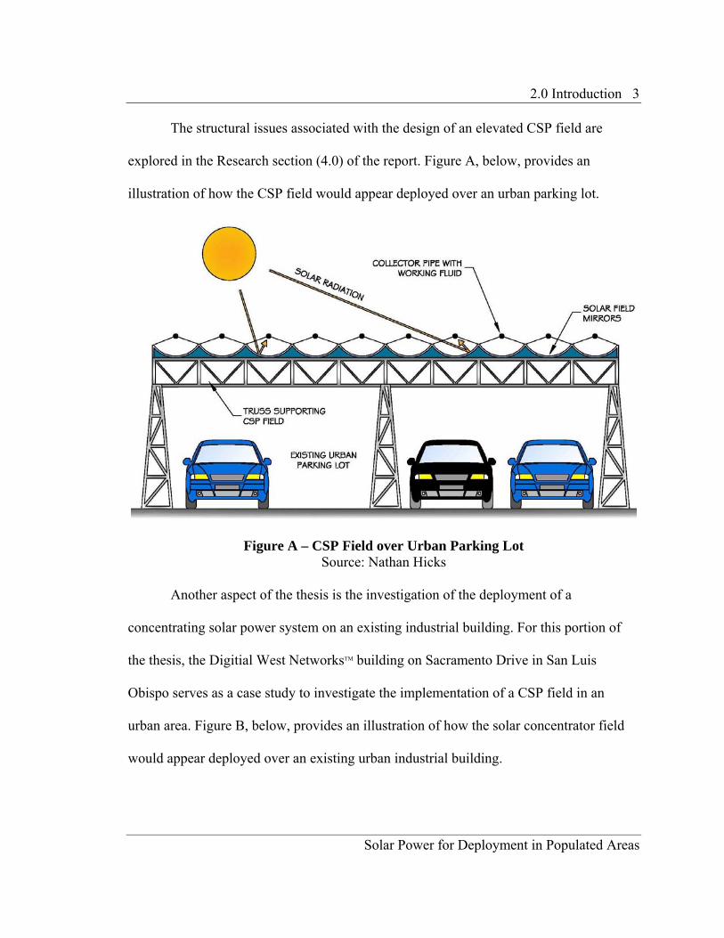
The structural issues associated with the design of an elevated CSP field are

explored in the Research section (4.0) of the report. Figure A, below, provides an

illustration of how the CSP field would appear deployed over an urban parking lot.

Figure A – CSP Field over Urban Parking Lot

Source: Nathan Hicks

Another aspect of the thesis is the investigation of the deployment of a

concentrating solar power system on an existing industrial building. For this portion of

the thesis, the Digitial West NetworksTM building on Sacramento Drive in San Luis

Obispo serves as a case study to investigate the implementation of a CSP field in an

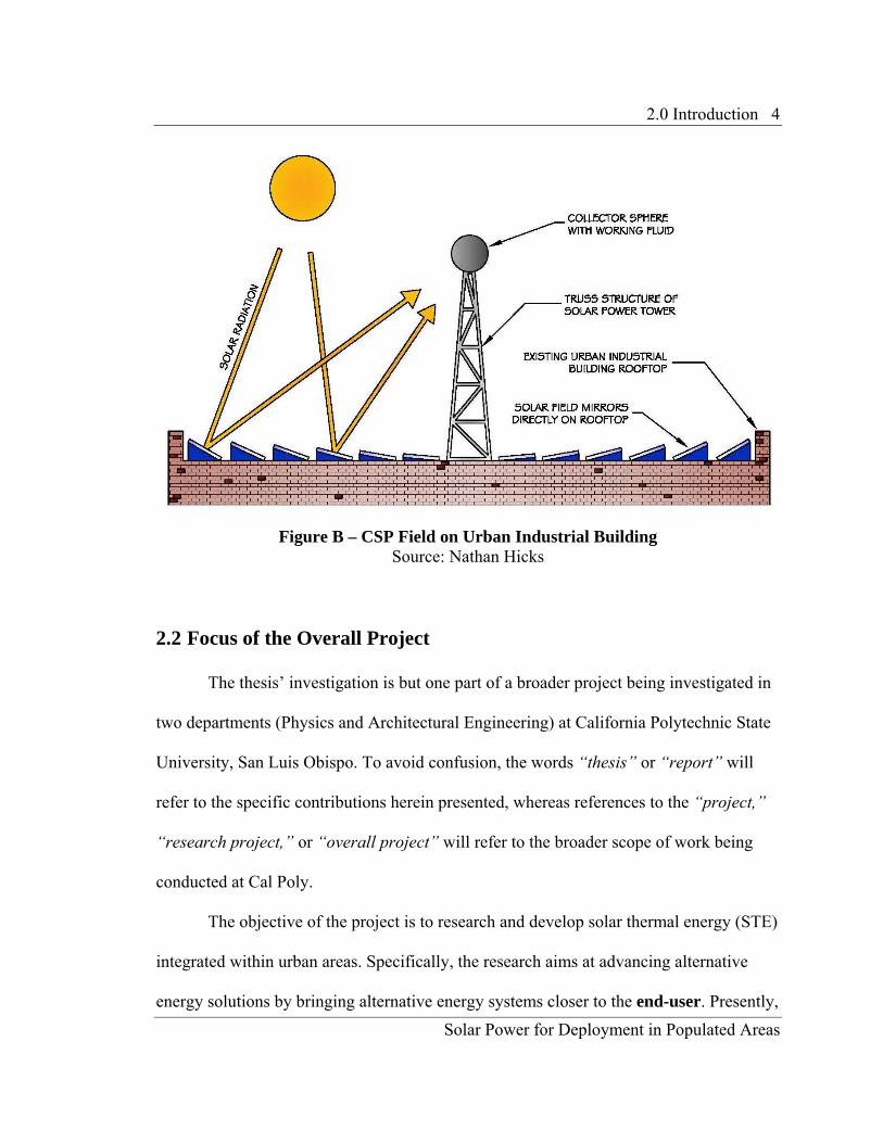
urban area. Figure B, below, provides an illustration of how the solar concentrator field

would appear deployed over an existing urban industrial building.

2.0 Introduction 4


Figure B – CSP Field on Urban Industrial Building


2.2 Focus of the Overall Project

The thesis’ investigation is but one part of a broader project being investigated in

two departments (Physics and Architectural Engineering) at California Polytechnic State

University, San Luis Obispo. To avoid confusion, the words “thesis” or “report” will

refer to the specific contributions herein presented, whereas references to the “project,”

“research project,” or “overall project” will refer to the broader scope of work being

conducted at Cal Poly.

The objective of the project is to research and develop solar thermal energy (STE)

integrated within urban areas. Specifically, the research aims at advancing alternative

energy solutions by bringing alternative energy systems closer to the end-user. Presently,

2.0 Introduction 5


urban end-users are offered a limited scope of on-site solar energy solutions, and the

solutions themselves are not economically feasible. Therefore, the project’s goal is to

investigate whether intermediate scale CSP fields have the potential to be the on-site

solar energy solution for urban areas and commercial buildings.

2.3 Relevance of Research

The fossil fuel trio of coal, oil, and natural gas provides more than three-quarters

of the world’s energy, today. Figure C, below, displays the predominant use of fossil

fuels worldwide as compared to other energy sources for 2004.

Figure C – Worldwide Energy Consumption Source: US Energy Information Administration

Despite this demand, intermittent concerns have been raised ever since the oil crisis of

the 1970s over the world’s continued dependence on fossil fuel. The expressed concerns

have dealt not only with the environmental impacts of fossil fuel use, but also with the

2.0 Introduction 6


finite nature of supplies (Boyle 2004), fueling an interest in finding a renewable energy

source for a sustainable future.

The goal of the overall project is to address the need for renewable energy sources

through the design of a solar concentrator field that provides cooling, heating, and power

services at a price consistent with present competitive technologies. In an effort to reach

this end, both the solar field and the structural system must be innovative in design.

While some individuals and corporations are willing to transition to renewable energy

sources out of concern for our natural resources and ecosystems, the majority will wait

until the solution is cost-effective. The wide-scale use of the solar concentrator field in

urban areas has the potential to be that cost-effective solution.

With the wide availability of suitable urban sites and the increasing scarcity of

conventional fuel sources, the solar concentrator field system could compete with fossil

fuel-based power in the future.

3.0 Background 7


3.0 BACKGROUND

The background section presents information on solar thermal energy (STE) that

is necessary for a complete understanding of this thesis.

Solar Thermal Energy (STE) is a technology for harnessing the sun’s solar energy

for thermal energy purposes. A majority of the solar thermal collectors currently

produced each year are low-temperature collectors that use water or air as a medium to

transfer heat to a final destination. The low-temperature collectors are common in

residential applications for space heating or the heating of swimming pools, but are

inefficient, in terms of return on investment, when used in commercial or large-scale

applications. As a result, the thesis will not deal with the low-temperature collectors, but

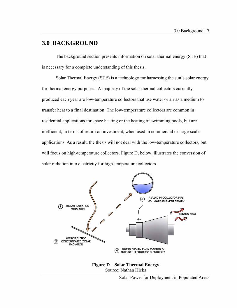
will focus on high-temperature collectors. Figure D, below, illustrates the conversion of

solar radiation into electricity for high-temperature collectors.

Figure D – Solar Thermal Energy Source: Nathan Hicks

3.0 Background 8


In the CSP field illustrated in the figure a mirror or lense is used to concentrate the sun’s

radiation onto a collector, creating a multi-sun effect. The working fluid in the collector is

then super heated to between 200° – 1000° C. As the fluid expands to a gaseous state, the

released energy powers a turbine that in turn produces electricity. In a vast majority of

solar thermal collectors, excess heat is wasted; however, by moving the solar thermal

collector near the end-user the waste heat can be used in heat storage, hot water

generation, and even air conditioning through the use of an absorption chiller.

STE technology should not be confused with the photovoltaic (PV) cells

commonly used in solar panels. Rather than converting the solar radiation into thermal

power, photovoltaic cells convert solar energy directly into electricity. While

photovoltaic panels are often adequate to meet the energy demands of a residential

building, they are not presently efficient for commercial use.

3.1 Early Solar Thermal Energy Systems

The idea of concentrating solar radiation in order to produce solar thermal energy

has been around for over 100 years.

In the late nineteenth century, France was struggling to meet energy demands as it

lacked an economical supply of coal. Addressing this lack of coal, Augustin Mouchot, a

French mathematics professor, began production on the first high-temperature solar

concentrators in the 1870s and 1880s. Over these years Mouchot and his assistant, Abel

Pifre, constructed and displayed a series of parabolic concentrators with a steam boiler

mounted at the focus of each concentrator. Solar radiation incident to the surface of the

parabolic dish was concentrated on the boiler, producing steam. The steam traveled down

3.0 Background 9


from the boiler through a series of pipes to a reciprocating engine, powering mechanical

work (Boyle 2004). Figure E, below, displays one of Pifre’s solar concentrators, which

was used to power a printing press.

Figure E – Pifre’s Solar Concentrator

Source: Boyle 2004

Although the concentrating solar power systems were widely acclaimed, it

became clear by the 1890s that the solar concentrators would be unable to compete with

coal in France. The parabolic dishes produced by Mouchot and Pifre were unable to

generate a concentration ratio high enough to create a competitive overall efficiency

(Boyle 2004).

3.0 Background 10


During this same era other attempts were made to mass-produce high-temperature

solar collectors, most notably by American entrepreneur Frank Shuman. After building

several prototypes and raising a substantial financial backing, Shuman began planning the

construction of 20,000 square miles of parabolic trough collectors in the Sahara Desert.

World War I broke out before construction could begin, and immediately after the war

the era of cheap oil began, effectively killing interest in high-temperature solar collectors

for half a century (Boyle 2004).

3.2 Contemporary Solar Thermal Energy Systems

Over the last few decades, interest in high-temperature solar collectors to use

solar thermal energy has increased once again. While these collectors are conceptually

the same, modern technology has allowed this new era of solar concentrators to reach

much higher overall efficiencies. The following sections will briefly overview three

concentrating solar power (CSP) systems that have the potential to be deployed in urban

areas.

3.2.1 Solar Power Towers

The first CSP system under consideration is the solar power tower. Solar power

towers use a large array of flat mirrors to concentrate solar radiation on a collector tower.

In the early 1980s the first solar power tower, Solar One, was constructed in Barstow,

California. The plant used synthetic oils to carry away the heat from the collector tower

to a steam boiler. In the 1990s Solar One was rebuilt to include heat storage, allowing the

production of electricity on a 24-hour basis. In 2005 a new tower project was completed

in Seville, Spain to explore the use of super-heated air as a transfer medium to a

3.0 Background 11


conventional steam turbine (Boyle 2004). Figure F, below, displays the solar power tower

in Seville and illustrates the intense concentration of the sun’s rays that can be achieved

with an array of flat mirrors.

Figure F – Seville Solar Power Tower

Source: NewEnergyDirection

Presently BrightSource Energy is developing solar power tower complexes in

both California’s Mojave Desert and Israel’s Negev Desert. Figure G, below, shows an

aerial view of the Ivanpah Solar Power Complex in the Mojave Desert.

Figure G – Ivanpah Solar Power Tower

Source: BrightSource Energy

3.0 Background 12


The 5-square-mile facility, illustrated above, began construction in 2009 and will be

completed in 2011, generating enough electricity to power 140,000 homes per year.

Solar power towers in an urban context would be on a much smaller scale than the

plants currently being built on desert floors. As a part of the thesis and the overall project,

the solar power tower is being explored as a possible method of deploying a solar

concentrator on the roof of an industrial building in an urban setting. The idea is that an

array of flat mirrors are added to the roof of existing industrial buildings of an adequate

size. The mirrors would then focus the sun’s rays onto a collector tower beginning, the

production of solar thermal energy.

From a structural perspective many issues must be addressed for the practical

integration of a collector tower in an urban area. First of all, the gravity system of the

industrial building on which the tower is being deployed must be investigated to ensure

that the building can resist the additional load of the mirrors, mechanical equipment, and

the tower itself. Additionally, in a seismically active region the tower must be engineered

to withstand the roof accelerations that would result from the ground accelerations of an

earthquake. As a relatively flexible column with a mass on the end, even small

accelerations at the base of the tower can lead to large and potentially destructive

displacements.

3.2.2 Solar Troughs

The second CSP system under consideration is solar concentrator troughs. Solar

concentrator troughs use long parabolic mirrors to focus the sun’s radiation on a

3.0 Background 13


continuous Dewar tube. The concentrated radiation heats up the fluid, commonly

synthetic oil, inside the tube as is shown in Figure H, below.

Figure H – Solar Trough

Source: trec-uk.org

The heat transfer fluid is then used to heat steam in a standard turbine generator (Boyle

2004). Often the troughs rotate to track the sun throughout the day and increase the

efficiency of the system. In such instances the solar troughs are oriented along a North-

South axis so that they can efficiently follow the sun from the east to the west horizon.

However, if the troughs are stationary and lack a tracking method, they are often oriented

along an East-West axis. With this stationary setup there is no need for tracking motors,

leading to a lighter, less mechanically complicated overall system, but this system

isconsequently far less efficient (Patel 2006).

3.0 Background 14


As a part of the thesis, the potential of an elevated solar trough system over urban

parking lots is being explored. The idea is that columns would support a frame-like

structure that would in turn carry the parabolic mirrors, tubing, and other mechanical

equipment for the solar concentrator system. Not only would the parabolic mirrors

provide solar thermal energy to the surrounding community, but the structure itself would

provide shielding from both sunlight and precipitation in the urban areas of deployment.

Structurally, the integration of a solar trough concentrator system over urban

parking lots raises key issues that are investigated in this thesis, including the wind

loading of open frame structures, the potential for destructive flutter behavior, and the

potential for destructive collapse. The key issues for both the industrial building and

parking lot structural systems will be discuessed in greater detail in the Research section

(4.0) of the report.

3.2.3 Concentrating Photovoltaics and Thermal (CPVT)

The third CSP system under consideration is concentrating photovoltaics (CPV).

Concentrating photovoltaics use lenses to concentrate the solar radiation onto a small area

of photovoltaic cells, as is shown on the following page in Figure I. To maximize the

concentration ratio, the CPV systems are often designed with tracking systems to stay in

line with the sun. While the photovoltaic cells convert the solar radiation into electricity

in the same manner as conventional panels, the photovoltaics in the concentrating system

are far more efficient; thus substantially fewer PV cells are required to produce the same

amount of electricity (Boyle 2004).

3.0 Background 15


Figure I – Concentrating Photovoltaics

Source: SolFocus

As a result of the high concentration of radiation, the cells in the concentrating

photovoltaic system have been plagued by overheating. In the past, the cells often needed

to be cooled either passively or actively to prevent this overheating. In order to address

this issue, Concentrating Photovoltaics and Thermal (CPVT) has emerged as a

technology that combines the electricity production of CPV systems with the thermal heat

production of STE systems. As the photovoltaic cells heat up, the system allows the flow

of a fluid to cool off the cells. Not only does the fluid absorb heat to allow the PV cells to

operate without overheating, but the heated fluid is also used in the production of solar

thermal energy. In this way both electricity and thermal energy are generated in a CPVT

system.

3.0 Background 16


The CPVT system has the potential to be integrated into both the elevated solar

trough system and the solar power tower system. As a part of the overall project, the

CPVT system is being explored by the physics team in order to establish whether or not

concentrating photovoltaics and thermal have the potential to be deployed in urban

environments.

4.0 Research 17


4.0 RESEARCH

The Research section investigates the key structural issues associated with the

integration of a solar concentrator field in an urban area, which are:

• Flutter

• Wind Loading of Open Frame Structures

• Performance-Based Design

In each of the sections, the key issue will be defined; the reason for an investigation of

the key issue will be explored; the research on the key issue will be presented; and finally

a conclusion will be made concerning the key issue’s impact on the thesis and overall

project.

4.1 Flutter

Flutter develops as the heaving (vertical) and torsional (twisting) motion of an

object are unified at single frequency. As the aerodynamic forces couple with the object’s

natural mode of vibration, a resulting rapid periodic motion emerges (Jakobsen and

Tanaka 2003). If the energy from the aerodynamic excitation exceeds the natural

dampening of the system, the level of vibration will increase. In such instances the self-

starting coupled flutter can result in potentially destructive vibrations (Jakobsen and

Tanaka 2003).

4.1.1 Reason for Investigation

Flutter was investigated to determine whether or not it was a phenomenon that

needed to be taken into account when designing the structural system for a CSP field. The

4.0 Research 18


thought was that flutter due to high winds might cause destructive behavior in the

elevated CSP structural model to be deployed over urban parking lots. In addition, there

was also a concern that flutter could cause destructive vibrations within the individual

elements, such as the mirrors, of the concentrating solar power field. As an open frame

structure, the interaction between the wind forces and the behavior of the building system

is more complex than for a similar closed structure.

4.1.2 Early Investigation of Flutter

The first exploration into flutter occurred in the first half of the nineteenth

century. On November 29, 1836 a section of the Brighton Chain Pier in East Sussex,

England failed in a storm. As local columnist George Bishop wrote,

About half-past twelve in the day the centre bridge seemed to have acquired through the force of the wind, a vibratory motion, which soon after, more or less affected the whole structure. At times the platform was raised to the level of the protecting iron rails at the sides of the Pier. Eventually one of the Towers began to rock, and the piles also to twist; and finally the platform of the third bridge was lifted up from its bed several feet, and, falling again — the suspension rods being unable to bear the stupendous strain — plunged into the stormy waters below (Bishop 1897).

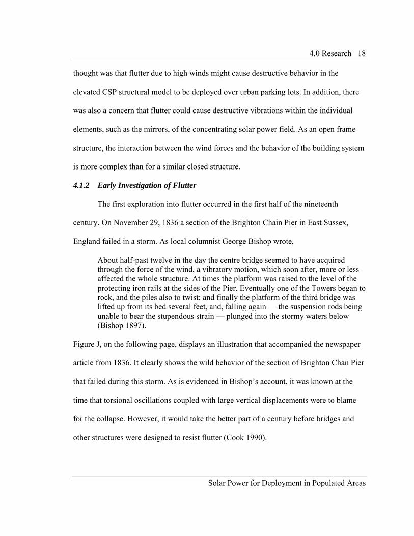
Figure J, on the following page, displays an illustration that accompanied the newspaper

article from 1836. It clearly shows the wild behavior of the section of Brighton Chan Pier

that failed during this storm. As is evidenced in Bishop’s account, it was known at the

time that torsional oscillations coupled with large vertical displacements were to blame

for the collapse. However, it would take the better part of a century before bridges and

other structures were designed to resist flutter (Cook 1990).

4.0 Research 19


Figure J – Brighton Chain Pier

Source: Bishop 1897

It wasn’t until the early 1900s with the development of the airplane that the

problem of flutter was readdressed. Individuals in the aeronautical field began

investigating the phenomenon of flutter after an aircraft designed by Samuel Pierpont

Langley broke apart shortly after takeoff on December 9, 1903. It was decided that a

complex torsional interaction between the airflow and the plane was at fault for the craft

breaking up, an interaction which we have come to know as flutter (Cook 1990).

The issue of instability in structures due to flutter wasn’t raised again until the

Tacoma Narrows Bridge Failure in 1940 (Matsumoto, et al. 2007). In the Tacoma

Narrows Bridge, as well as other long span bridges, the weak torsional rigidity ultimately

made the bridges susceptible to a strong wind flow. Over the years, as bridges have

employed the use of ever stronger and lighter building materials, there has been a

significant decrease in the natural frequency of these structures. In addition, the evolution

to stronger and lighter materials has resulted in a decrease in the ratio between the

4.0 Research 20


fundamental torsional and vertical mode frequencies, making long span bridges even

more vulnerable to flutter instability (Bartoli and Righi 2006). Research by bridge

engineers, such as Farquharsen and Karman, over the last half-century has led to the

formulation of high order differential equations to calculate the critical wind speeds at

which lift and pitching moment are maximized (Matsumoto, et al. 2008). These

differential equations have enabled the design of bridges less likely to experience

unstable torsional, dynamic responses. Furthermore, research in bridge engineering has

revealed that in the wind velocity range of interest for bridge design, the flow around

bluff body bridge sections (bridge deck) is not agreeable with the quasi-steady flow

theory. The use of turbulent flow as opposed to steady flow in bridge design actually

reduces the amplitude of the motion, since the lack of correlation of the incoming wind

introduces an aerodynamic damping effect (Bartoli and Righi 2006).

4.1.3 Current Investigation of Flutter

Outside of aeronautics and bridge engineering, very little research has been done

on the issue of flutter instability. One of the compelling reasons to investigate flutter as a

part of this thesis is due to the similarities between the cross section of the proposed

elevated CSP field and the cross section of a typical bridge. In bridge engineering the

ratio of the length or breadth of a bridge section (B), to the depth of the section (D) is an

indicator of how susceptible a structure is to flutter. A higher B/D ratio often translates to

a weak torsional rigidity and a structure potentially more susceptible to destructive

flutter. As Figure K, below, illustrates, the elevated CSP field for deployment over urban

parking lots has a B/D ratio larger than that of a bridge section.

4.0 Research 21


Figure K – B/D Ratio Comparison


While this may seem to be cause for concern, differences between the elevated CSP field

and the bridge section need to examined before arriving at any conclusions.

The first key difference is that a major contributor to the weak torsional rigidity of

many bridges is their relatively long span in relation to the breadth of the section. The

elevated CSP field’s span to breadth ratio is not as severe as that seen in bridges, and

therefore more torsional rigidity is provided. However, the defining difference between

the solar field model and a long span bridge is the fact that the CSP field is anchored to

the ground by columns. Although not perfectly rigid, these columns limit the overall

heaving and torsional displacements of the structure to infinitesimal amounts. As Figure

L, on the following page, displays a bridge develops flutter as the vertical and torsional

motion are unified at a single frequency. In the elevated CSP field the vertical and

torsional motion do not develop. The columns that support the structural system restrict

the CSP field from any large displacements in the vertical direction.

4.0 Research 22


Figure L – Heaving and Torsional Motion


4.1.4 Conclusion on Flutter

The thesis concludes that flutter is not an issue that need be addressed in the

modeling of the overall structural system for the elevated CSP field being deployed over

urban parking lots. The columns supporting the CSP field provide enough vertical

rigidity to resist large vertical displacements due to dynamic wind loading. Future testing

of the mirrors, solar troughs, and supporting infrastructure in moderate wind speeds will

be needed to establish what type of support is necessary to resist the potentially

destructive vibrations of flutter within individual components of the CSP field.

4.2 Wind Loading of Open Frame Structures

The basis and procedures for calculating wind induced forces on conventional and

enclosed structures are well documented in the engineering literature, perhaps most

notably in the ASCE 7-05 and its predecessor documents. The provisions set forth in the

4.0 Research 23


ASCE 7 have been adopted by organizations in the development of their building codes.

One such building code to adopt the ASCE 7 is the International Building Code, which is

the model building code adopted throughout most of the United States.

The scope of the ASCE 7 states, “This standard provides minimum load

requirements for the design of buildings and other structures that are subject to building

code requirements.” However, even a task committee from the American Society of Civil

Engineers (ASCE) acknowledged that the ASCE 7 does not adequately address open

frame structures. Lacking a uniform method, the industry has developed numerous design

practices to calculate the wind loading on open frame structures, all of which can vary

greatly in the resulting wind induced forces (ASCE 1997).


The concentrating solar power field deployed over urban parking lots calls for an

elevated structural system. The elevated CSP system consists of solar troughs running

over a frame-like structure that is supported above the parking lot by columns. The

structure would likely lack any exterior cladding and thus would behave as an open frame

structure. Due to the structure’s lightweight construction, it becomes increasingly likely

that the lateral forces in the system would be governed by wind rather than earthquake

even in high seismic regions of California. It is therefore essential that in the design of

the lateral force resisting system an acceptable method be found for calculating the wind

forces on an open frame structure.

4.0 Research 24


4.2.2 Current Investigation of Wind Loading

Chapter 6 of the ASCE 7-05 presents methods for calculating the wind-induced

lateral forces on a building. The basic principles and procedures behind the methods are

similar, and for the purpose of this thesis are presented in a simplified manner. The first

step in the design procedure is to determine the basic wind speed, V, in accordance with

the values shown on Figure M, below.

Figure M – Basic Wind Speed

Source: ASCE 7-05

The basic wind speed can then be translated into a simplified design wind pressure, pS30,

using an accompanying figure in the chapter. The final design wind pressure for the

system, ps, can be calculated using Equation 1, below:

4.0 Research 25


ps = λ(Kzt)(I)(pS30), Eq. 1

where λ is the adjustment factor for building ht. and exposure (dimensionless), Kzt is the wind topographic adjustment factor (dimensionless), I is the importance factor (dimensionless), and pS30 is the simplified design wind pressure (psf). The final design wind pressure, ps, is then applied to projections of the building surfaces

in order to determine the total base shear (ASCE 7-05).

The shortcoming of the ASCE 7-05 wind design procedure is illustrated in plan

view in Figure N, below.

Figure N – Wind Direction


As the solidity ratio, ε, of the frame decreases, the maximum force on the open frame

structure no longer occurs when the wind direction is normal to the set of frames. The

solidity ratio is defined in Equation 2, below:

ε = As/Ag, Eq. 2

where As is the gross projected area of the solid wall (ft2), and Ag is the gross projected area of the wall including openings (ft2).

4.0 Research 26


At a wind angle of attack, α, equal to 0° in an open frame structure, the columns

at the front of the structure in effect shield the back columns in the frame from

experiencing any wind pressure. As a result the design wind pressure is only applied to

the gross projected of the solid wall, Ag. As α increases beyond 0° the lateral force

component normal to the frame will decrease, but the projected area that the wind

pressure acts on will likely increase. Eventually an α is found that maximizes the lateral

force on the open frame structure. In a guideline for the wind loading of open frame

structures published by the ASCE, the task committee states

Although the wind direction is nominally considered as being normal to the set of frames under construction, the maximum force coefficient occurs when the wind is not normal to the frames. The angle at which the maximum force coefficient occurs varies with the dimensions of the structure, the solidity, number of frames, and frame spacing (ASCE 7-05).

The ASCE task committee, realizing the deficiency in the ASCE 7-05 for wind loading of

open frame structures, began work on a uniformly accepted design guideline for

calculating the wind-induced forces on open frame structures. Rather than using the

maximum α in order to calculate the wind-induced base shear, the task committee

devised a method in which the wind pressure calculated from the ASCE 7-05 was

modified by a force coefficient and a gust effect factor. The resulting Equation 3, below,

gives the base shear due to wind, F, on an open frame structure:

F = ps (G) (Cf) (As) , Eq. 3

where ps is the final design wind pressure (psf), G is the gust effect factor (dimensionless), Cf is the force coefficient (dimensionless), and As is the gross projected area of the solid wall (ft2).

4.0 Research 27


The gust effect factor, G, can be calculated using the ASCE 7-05, however the force

coefficient, Cf, is calculated using the ASCE task committee design guide and is

presented in Equation 4:

Cf = CDg / ε , Eq. 4

where CDg is the force coefficient on the wall’s gross area (dimensionless), and ε is the solidity ratio (dimensionless).

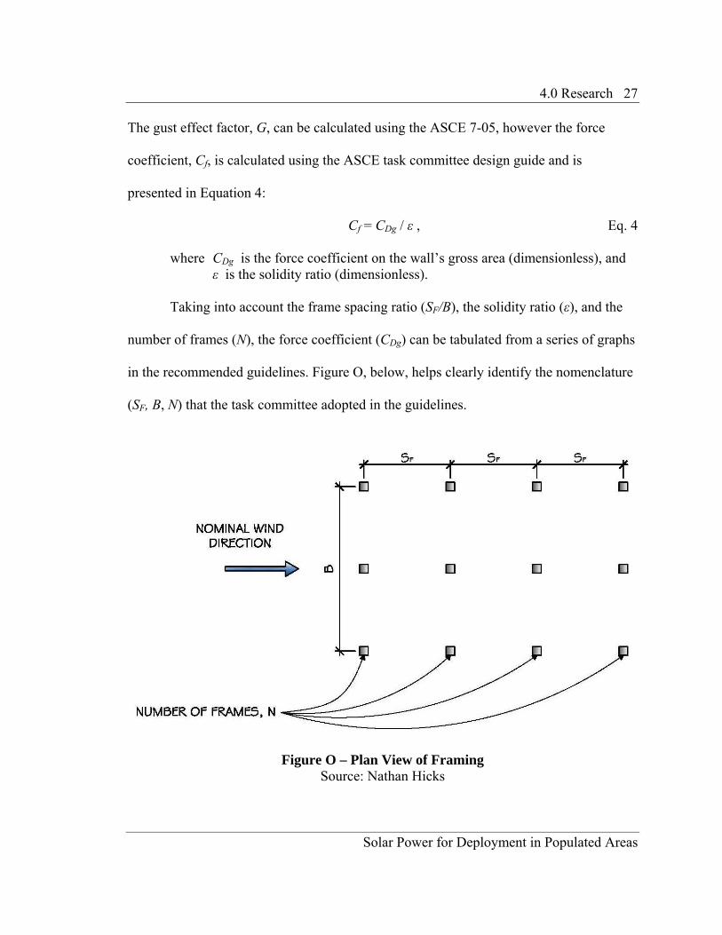
Taking into account the frame spacing ratio (SF/B), the solidity ratio (ε), and the

number of frames (N), the force coefficient (CDg) can be tabulated from a series of graphs

in the recommended guidelines. Figure O, below, helps clearly identify the nomenclature

(SF, B, N) that the task committee adopted in the guidelines.

Figure O – Plan View of Framing


4.0 Research 28


Figure O provides a hypothetical open frame structure in plan view and identifies

the variables that are needed in order to interpret the ASCE task committee’s design

guidelines force coefficient (CDg) graphs.

Figure P, on the following page, displays the force coefficient graphs for four

different frame spacing ratios (SF/B = .1, .2, .33, .5). For frame spacing ratios in between

the four frame spacing ratios, linear interpolation can be used in order to identify the

force coefficient on the gross area (CDg). Each graph in Figure P plots the force

coefficient (CDg) as a function of the frame solidity ratio (ε) for structures with anywhere

from 2 – 12 frames (N).

4.0 Research 29


Figure P – Force Coefficient

Source: (ASCE 1997)

4.0 Research 30


4.2.3 Conclusion on Wind Loading

It is the recommendation of this thesis that the wind-induced forces on an open

frame structure deployed over an urban parking lot be calculated using the ASCE 7-05 in

combination with the recommended guidelines set forth by the ASCE task committee in

Wind Loads and Anchor Bolt Design for Petrochemical Facilities. An additional

consideration with the wind loading of open frame structures is that the design load cases

must take into account that the maximum wind load occurs when α > 0. As a result it is

the recommendation of both the task committee and this thesis that the designer take the

total wind force acting on the structure in a given direction and simultaneously apply

50% of the total wind force along the other axis.

4.3 Performance-Based Design

Presently in the United States, design is regulated based on national model

building codes. When adopted and enforced by local authorities, building codes are

intended to establish minimum requirements for providing safety to life and property

from hazards such as wind, earthquake, and fire. The building code’s goal is

accomplished through prescriptive requirements, developed over the years by the

performance assessment of buildings after a hazard (FEMA 445). The prescriptive

criteria of building codes provide an assurance that design professionals will avoid

repeating mistakes. In addition, building codes facilitate a simple and relatively rapid

design, permit, and construction process, in which the liability of the design professional

is minimized (Hamburger 2009).

4.0 Research 31


Although the prescriptive criteria of model building codes are intended to result in

buildings capable of providing a minimum of life safety performance, actual performance

of individual building designs is not traditionally assessed. The lack of an assessment of

building performance in the codes has led to a public misconception of how buildings

will respond to a major seismic event. While the public may expect limited structural

damage after a large seismic event, this expectation is not in accord with the intent of the

building code. Historically, the intent of building code seismic provisions has been to

provide buildings with an ability to withstand intense ground shaking without collapse.

However even without collapse there could potentially be significant structural and

nonstructural damage (FEMA 445). As the 1997 Uniform Building Code (UBC) states,

the purpose of the code is “…to safeguard against major structural failures and loss of

life, not to limit damage or maintain function.”

Earthquakes at the end of the twentieth century, such as the 1994 Northridge

Earthquake, led to the recognition that “the level of structural and nonstructural damage

that could occur in code-compliant buildings may not be consistent with public notions of

acceptable performance” (FEMA 445). While the Northridge Earthquake resulted in only

fifty-seven deaths, the earthquake caused an estimated $20 billion in damage, according

to Pacific Earthquake Engineering Research Center (PEER). While the code was

relatively successful in safeguarding against loss of life, the money and time lost from the

damage and loss of function of building, was unacceptable. As a result, the engineering

community has moved toward predictive methods for assessing seismic performance, and

4.0 Research 32


the development of what is known in the engineering community as performance-based

design (PBD).


Performance-based design evaluates how a building is likely to perform, given a

potential hazard. The performance, which is detailed further in Table A, can be measured

in terms of deflections, plastic rotations, and nonstructural appearance, among other

things. PBD was investigated to determine if it was an appropriate method to use in the

design of CSP fields deployed directly on the roof of urban industrial buildings. The use

of PBD allows the design professional to clearly communicate to an owner the expected

performance of the rooftop solar power tower to a range of seismic events.

4.3.2 Early Investigation of Performance-Based Design

Traditionally in performance-based design, the target building performance levels

have been defined as:

• Operational Performance

• Immediate Occupancy Performance

• Life Safety Performance

• Collapse Prevention Performance

Table A, on the following page, reveals the expected post-earthquake structural and

nonstructural damage associated with specific performance levels.

4.0 Research 33


Table A – Damage vs. Building Performance Level

Source: FEMA 356

The post-earthquake damage state of the building ranges from severe for collapse

prevention performance, to very light for operational performance.

Building performance objectives are formed when selecting target building

performance levels for a broad range of earthquake hazard levels. For instance in PBD,

the performance objectives might dictate that a building be designed to an operational

performance level for relatively minor or frequent earthquakes, and a collapse prevention

performance level for major or very rare earthquakes. The earthquake hazard levels are

based upon a probabilistic approach to earthquake severity and are measured in terms of

the mean return periods of the earthquakes, or in other words the average number of years

between events of similar severity. Table B, on the following page, provides the

probabilistic earthquake hazard levels commonly used in FEMA and ASCE documents

(FEMA 356).

4.0 Research 34


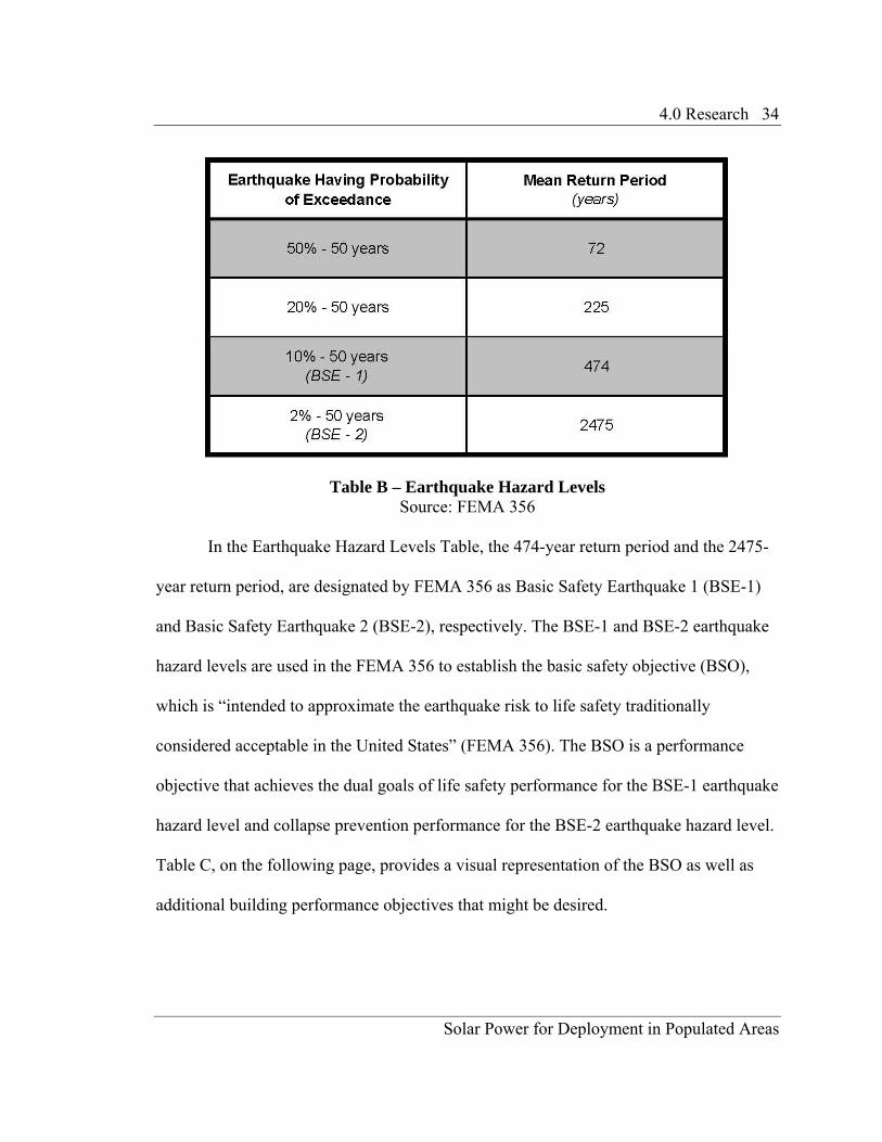
Table B – Earthquake Hazard Levels

Source: FEMA 356

In the Earthquake Hazard Levels Table, the 474-year return period and the 2475-

year return period, are designated by FEMA 356 as Basic Safety Earthquake 1 (BSE-1)

and Basic Safety Earthquake 2 (BSE-2), respectively. The BSE-1 and BSE-2 earthquake

hazard levels are used in the FEMA 356 to establish the basic safety objective (BSO),

which is “intended to approximate the earthquake risk to life safety traditionally

considered acceptable in the United States” (FEMA 356). The BSO is a performance

objective that achieves the dual goals of life safety performance for the BSE-1 earthquake

hazard level and collapse prevention performance for the BSE-2 earthquake hazard level.

Table C, on the following page, provides a visual representation of the BSO as well as

additional building performance objectives that might be desired.

4.0 Research 35


Table C – Building Performance Objectives

Source: Vision 2000

As is shown in the Performance Objectives Table, the basic safety objectives

outlined in the FEMA 356 are consistent with the minimum performance objectives

outlined in other performance-based design standards. If the building is designed to a

performance exceeding the BSO, it is termed an enhanced performance objective, and if

the building is designed to a performance less that that of the BSO, it is termed a limited

performance objective (FEMA 356).

After performance objectives for a building are determined collaboratively by the

owner, design professionals, and building officials a preliminary building design is

4.0 Research 36


developed. After the preliminary design PBD becomes an iterative process. The flow

diagram for PBD is illustrated in Figure Q, shown below.

Figure Q – Performance-Based Design Flow Diagram

Source: FEMA 445

Following the preliminary building design, the performance of the building is assessed,

and if it meets the objectives the process is complete. If the building does not meet the

objectives, the design is revised until it is able to meet the objectives (FEMA 445).

4.3.3 Current Investigation of Performance-Based Design

In a structure the seismic base shear, V, from an earthquake can be determined by

multiplying the mass of the structure, W, by the acceleration at the base of the structure,

Cs. Although earthquakes result from a rupture in the earth’s crust miles under the

ground, Cs considers the motion at the surface of the earth as well as the potential for

4.0 Research 37


resonance in the structure. Equation 5, below, presents the seismic base shear equation

from the ASCE 7:

,WCV s= Eq. 5

where V = Seismic base shear (k), Cs = Seismic response coefficient (g), and W = Effective seismic weight (k/g). The ground acceleration, Cs, is based upon ground motion data from the United States

Geological Survey (USGS) for a 474 year return period earthquake (BSE-1) modified by

the ASCE 7 to take into account the soil conditions and structure period (ASCE 7-05).

The structural challenge associated with deploying a CSP field on the rooftop of

an urban industrial building is that the roof accelerations acting at the base of the solar

power tower cannot be calculated directly from the USGS ground motion data. The ASCE

7 does not provide procedures for calculating accelerations at floor or roof levels, and

thus an alternative design guideline was needed to address the seismic design of flexibly

mounted equipment (solar power tower) on a building. The Seismic Design Guidelines

for Essential Buildings, a technical manual published by Office of the Chief of Engineers,

United States Army, was found to provide a basic performance-based procedure for

designing flexibly mounted equipment on a building, and will be drawn upon in the

design of the solar power tower. The premise of the guideline is quantifying the

accelerations at the roof from the ground accelerations at the foundation. Figure R,

below, displays the relationship between the ground accelerations, the amplified roof

accelerations, and the solar power tower, for an urban industrial building.

4.0 Research 38


Figure R – Response of Flexibly Mounted Equipment


Chapter 6 of Seismic Design Guidelines for Essential Buildings, “prescribes the

criteria for non-structural elements that must remain intact or functional after a major

seismic disturbance. The provisions include the determination of the seismic forces to be

applied to the elements and the determination of the deformations that the elements will

withstand” (United States 1986). The military design guideline provides two performance

objectives for the flexibly mounted equipment. In the event of a 50% in 50 years

earthquake (72-year return period) the element will be designed for an operational

performance level, and in a 10% in 100 years earthquake (950-year return period) the

element will be designed for a collapse prevention performance level. In the design

guideline, the 72-year return period earthquake is designated as EQ-1 and the 950-year

return period earthquake is designated as EQ-2.

4.0 Research 39


In order to design a solar power tower for both the 72-year (EQ-1) and 950-year

(EQ-2) earthquake hazard levels, the corresponding seismic base shear for each event

must be calculated. As Equation 5 (on page 37) illustrates, the seismic base shear of the

flexibly mounted equipment (solar power tower) is based upon the acceleration at the

base of the tower and the effective seismic weight of the tower. The effective seismic

weight can be calculated by summating the weights of the structural and mechanical

systems, including the working fluid in the solar power tower. However, to calculate the

design acceleration at the base of the tower (roof of the industrial building), a roof

response spectrum for each seismic event needs to be developed. The roof response

spectrum plots the maximum design acceleration at the roof, Sfa, as a function of the solar

tower period.

In order to generate the roof response spectra, the basic procedure from Chapter 6

of the Seismic Design Guidelines for Essential Buildings will be employed, with

modifications to take advantage of up-to-date ground motion data and three-dimensional

computer modeling. To clearly convey the design procedures for generating a roof

response spectrum, the Digitial West NetworksTM industrial building on Sacramento Drive

in San Luis Obispo will serve as a case study for deploying a solar power tower.

4.3.4 Performance-Based Design Case Study

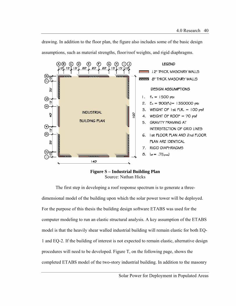
A basic floor plan of the industrial building on Sacramento Drive is provided in

Figure S, on the following page. The figure displays the dimensioned floor plan, with a

legend that designates the location of both the 8” and 12” thick masonry walls on the plan

4.0 Research 40


drawing. In addition to the floor plan, the figure also includes some of the basic design

assumptions, such as material strengths, floor/roof weights, and rigid diaphragms.

Figure S – Industrial Building Plan


The first step in developing a roof response spectrum is to generate a three-

dimensional model of the building upon which the solar power tower will be deployed.

For the purpose of this thesis the building design software ETABS was used for the

computer modeling to run an elastic structural analysis. A key assumption of the ETABS

model is that the heavily shear walled industrial building will remain elastic for both EQ-

1 and EQ-2. If the building of interest is not expected to remain elastic, alternative design

procedures will need to be developed. Figure T, on the following page, shows the

completed ETABS model of the two-story industrial building. In addition to the masonry

4.0 Research 41


walls along the exterior of the building, gravity framing was included at the intersection

of all grid lines to restrain the vertical movement of the diaphragm and allow the model

to display distinct mode shapes.

Figure T – ETABS Model


After completing the model and running the analysis, the next step is to record the

mass that was assigned to each level of the structure, mi, and the period of all modes, Tm.

Table D, on the following page, displays the mass assigned to both the floor level and the

roof level for the case study industrial building. The mass assigned to level 1, or the floor

level, is based upon a dead load of 100 psf, and the mass assigned to level 2, or the roof

4.0 Research 42


level, is based upon a dead load of 70 psf. Within the model the mass of the exterior

masonry walls as well as the gravity framing has been lumped into the dead load applied

to the diaphragm.

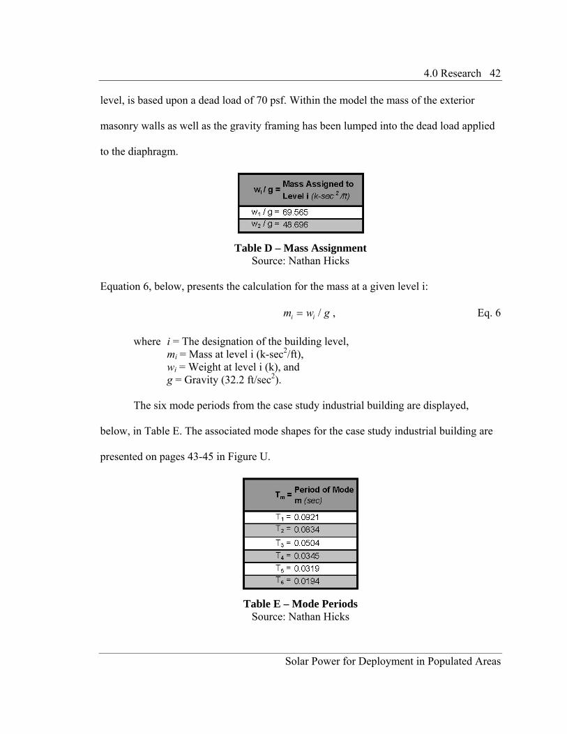
Table D – Mass Assignment


Equation 6, below, presents the calculation for the mass at a given level i:

gwm ii /= , Eq. 6

where i = The designation of the building level, mi = Mass at level i (k-sec2/ft), wi = Weight at level i (k), and g = Gravity (32.2 ft/sec2). The six mode periods from the case study industrial building are displayed,

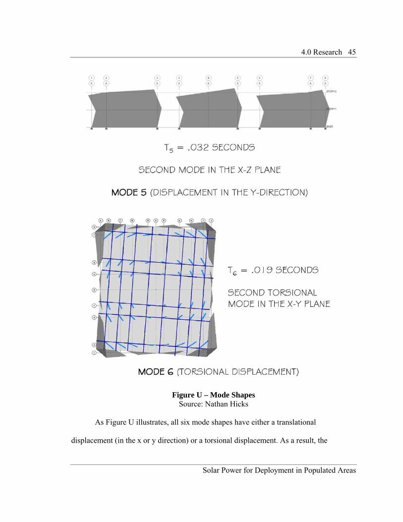
below, in Table E. The associated mode shapes for the case study industrial building are

presented on pages 43-45 in Figure U.

Table E – Mode Periods


4.0 Research 43


4.0 Research 44


4.0 Research 45


Figure U – Mode Shapes


As Figure U illustrates, all six mode shapes have either a translational

displacement (in the x or y direction) or a torsional displacement. As a result, the

4.0 Research 46


computer program can display the relative amplitude of the displacements, imφ , at all

levels, i, for every mode, m. The modal displacement amplitudes need to be recorded as

shown in Table F, on the following page, for modes 1 through 6 at both the floor level

and the roof level for the case study industrial building.

Table F – Amplitude of Modal Displacements


In the case study, the amplitude of displacements in the x-direction are used for modes 1

and 4, the amplitude of displacements in the y-direction are used for modes 2 and 5, and

the amplitude of rotations are used for the torsional modes 3 and 6.

The amplitude values from Table F are then used in the calculation of the modal

participation factor, PFxm, at the roof level for modes 1 through 6. Equation 7, on the

following page, presents the calculation for the modal participation factor from the

United States Army design guideline:

4.0 Research 47


( )

( )( )xm

n

iim

i

n

iim

i

xm

gw

gw

PF φ

φ

φ

⎟⎟⎟⎟⎟

⎠

⎞

⎜⎜⎜⎜⎜

⎝

⎛

⎟⎟⎠

⎞⎜⎜⎝

⎛

⎟⎟⎠

⎞⎜⎜⎝

⎛

=

∑

∑

=

=2

1

1 , Eq. 7

where x = Building level of interest, n = Total number of building levels, i = The designation of the building level, wi = Weight at level i (k), g = Gravity (32.2 ft/sec2), imφ = Amplitude of mode m at level i, xmφ = Amplitude of mode m at level x, and PFxm = Modal participation factor at level x for mode m. The modal participation factors at the roof level (x = 2) for the case study

industrial building are shown below in Table G.

Table G – Modal Participation Factors


The next step in developing the roof response spectra is to calculate the EQ-1 and

EQ-2 spectral acceleration, Sam, at the ground level, for every mode, m. The 50% - 50

year and 10% - 100 year earthquake hazard levels chosen for the performance objectives

by the US Army design guideline do not match up with the design level earthquake

(BSE-1) or maximum considered earthquake (BSE-2) that are typically used by the ASCE

4.0 Research 48


7, USGS, or FEMA. The BSE-1 corresponds to a 10% - 50 year earthquake and the BSE-

2 corresponds to a 2% - 50 year earthquake.

Using a ground motion calculator provided on the USGS website, the spectral

response acceleration at the ground level for short periods and at 1 second for both BSE-1

(SDS & SD1) and the BSE-2 (SMS & SM1) can be found. The ground motion calculator, as

shown in Figure V, below, obtains the four spectral acceleration values after the user

inputs the zip code of the building location and the site class.

Figure V – USGS Ground Motion Calculator

Source: USGS

One of the keys in converting the spectral accelerations from the BSE-1 and BSE-

2 hazard level earthquakes (SDS, SD1, SMS, SM1) to spectral accelerations for the EQ-1 and

4.0 Research 49


EQ-2 hazard level earthquakes is the establishment of the mean return period of the

hazard levels. Equation 8, below, presents the mean return period equation from FEMA

356:

( )EYR PYP −−= 1ln , Eq. 8

where Y = Exposure time for the desired earthquake hazard level (years), PEY = Probability of excceedance (expressed as a decimal) in time Y, and PR = Mean return period of the earthquake hazard level (years). After the mean return period has been obtained for EQ-1 (72 years) and EQ-2

(949 years), the spectral response acceleration at the ground level for these hazard levels

can be obtained from equations in section 1.6.1.3 of FEMA 356. If the mean return period

is between 475 years (BSE-1) and 2475 years (BSE-2) the spectral acceleration, Sxi, can

be determined from Equation 9:

( ) ( ) ( ) ( )[ ] ( )[ ]73.3ln606.lnlnlnln 121 −−+= −−− RBSEDiBSEMiBSEDixi PSSSS , Eq. 9

where PR = Mean return period of the earthquake hazard level (years), i = s or 1, 1−BSEDiS = Spectral acceleration parameter for BSE-1 hazard level (g), 2−BSEMiS = Spectral accel. parameter for BSE-2 hazard level (g), and XiS = Spectral acceleration parameter for EQ-1 or EQ-2 hazard level (g). If the mean return period is less than 475 years the spectral acceleration, Sxi, can

be determined from Equation 10 on the following page:

4.0 Research 50


nR

BSExixiPSS ⎟

⎠⎞

⎜⎝⎛= − 4751 , Eq. 10

where PR = Mean return period of the earthquake hazard level (years), i = s or 1, 1−BSEDiS = Spectral acceleration parameter for BSE-1 hazard level (g), XiS = Spectral accel. parameter for EQ-1 or EQ-2 hazard level (g), and n = Value obtained from Table H, which is Table 1-2 in FEMA 356.

As a part of Equation 10, a value of exponent n is provided by Table 1-2 in FEMA

356. That table has been reproduced, below, in the thesis as Table H.

Table H – Values of Exponent n

Source: FEMA 356

After the spectral accelerations have been calculated for the EQ-1 and EQ-2

hazard levels the design response spectra at the ground level of the industrial building can

be generated. Figure W, on the followng, displays the design response spectra for the

case study industrial building.

4.0 Research 51


Figure W – Design Response Spectrum at Ground Level


Based upon the period of the building, Tm, the design response spectrum can be

divided into three regions. If Tm < T0, then the building is in the constant velocity region

of the design spectra and the modal spectral acceleration, Sam, can be calculated using

Equation 11 (ASCE 7-05):

( )( )06.4. TTSS mXSam += , Eq. 11

where Sam = Spectral acceleration of mode m (g), SXS = 5 percent damped, spectral response acceleration parameter at short periods (g), Tm = Building period at mode m (sec), and T0 = .2(SD1/SDS).

4.0 Research 52


If T0 ≤ Tm ≤ TS the building is in the constant acceleration region of the design spectra

and the modal spectral acceleration, Sam, can be calculated using Equation 12

(ASCE 7-05):

Sam = SXS, Eq. 12

where Sam = Spectral acceleration of mode m (g), SXS = 5 percent damped, spectral response acceleration parameter at short periods (g), and TS = SD1/SDS (sec). If Tm < Ts the building is in the constant displacement region of the design spectra and the

modal spectral acceleration, Sam, can be calculated using Equation 13 (ASCE 7-05):

Sam = SX1/Tm, Eq. 13

where Sam = Spectral acceleration of mode m (g), SX1 = 5 percent damped, spectral response acceleration parameter at a period of 1 second (g), and Tm = Building period at mode m (sec), Using the building period for modes 1 through 6, Tm, and the design response

spectrum shown in Figure W (page 51), the spectral acceleration, Sam, of modes 1 through

6 can be calculated. In the case study industrial building, the period of all modes was less

than T0, and thus the modal spectral acceleration at the ground level could be calculated

using Equation 11. Table I, on the following page, displays a summary of the modal

spectral accelerations for both EQ-1 and EQ-2 for the case study industrial building.

4.0 Research 53


Table I – Modal Spectral Accelerations


Using the modal spectral acceleration at the ground level, Sam, the modal story

acceleration at the roof, axm, (x = 2) can be calculated using Equation 14:

( )amxmxm SPFa = , Eq. 14

where axm = Modal story acceleration at level x for mode m (g), PFxm = Modal participation factor (see Eq. 7 on page 47), and Sam = Spectral acceleration of mode m (g). For each earthquake hazard level, the maximum acceleration at level x, ax max, can be

found using the square-root-of-sum-of-squares (SRSS) rule for modal combination. The

SRSS rule is expressed, on the following page in Equation 15:

∑= 2max xmx aa , Eq. 15

where ax max = Maximum story acceleration at level x (g), and axm = Modal story acceleration at level x for mode m (g). A summary of the modal story accelerations, at the roof, for the case study industrial

building, along with the maximum roof acceleration is presented, below, in Table J.

4.0 Research 54


Table J – Modal Story Acceleration


Using the modal story accelerations at the roof a plot of the spectral roof response

acceleration, Sfa, versus the period of the solar tower, Ta, can be developed with the aid of

Figure X, which is located on the following page. Figure X plots the design magnification

factor as a function of the ratio of the solar tower period, Ta, over the modal building

period, Tm (United States 1986). Equation 16 and 17, shown below, can be used in

combination with Figure X in order to calculate the roof response spectrum plot for each

mode:

Ta = (Ta/Tm)Tm , Eq. 16

Sfa = axm(Magnification Factor), Eq. 17

where Ta = Period of solar tower or other flexibly mounted equipment (sec), Tm = Building period at mode m (sec), Ta/Tm = Period Ratio from Figure X, Sfa = Spectral roof response acceleration (g), axm = Modal story acceleration at level x for mode m (g), and Magnification Factor = Reference y-axis of Figure X on page 55.

4.0 Research 55


Figure X – Design Magnification Factor vs. Period Ratio

Source: United States 1986

Table K, below, illustrates the tabulation of the pertinent data required for such a plot for

the first mode of the case study industrial building.

Table K – First Mode Spectral Roof Response Acceleration Tabulation


4.0 Research 56


The tabulation shown for the first mode in Table K needs to be repeated for each

modal period and modal story acceleration in order to produce a curve on the roof

response spectrum for each mode. The roof response spectrum also needs to include a

horizontal line intersecting the coordinate at Sfa = ax max, where ax max is the maximum

floor acceleration from Eq. 15. The final roof response spectrum is defined by the

envelope of the aforementioned curves established by Eq. 16 and 17 as well as the

horizontal line established by Eq. 15 (United States 1986). For the case study industrial

building, it was necessary to develop a roof response spectrum for the service level

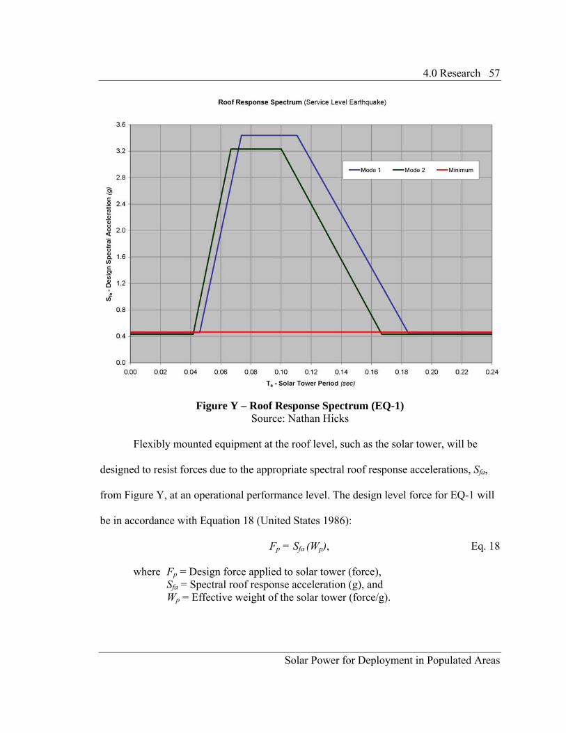
earthquake, EQ-1, and the maximum considered earthquake, EQ-2. Figure Y, on the

following page, displays the completed roof response spectra of the case study industrial

building for EQ-1.

4.0 Research 57


Figure Y – Roof Response Spectrum (EQ-1)


Flexibly mounted equipment at the roof level, such as the solar tower, will be

designed to resist forces due to the appropriate spectral roof response accelerations, Sfa,

from Figure Y, at an operational performance level. The design level force for EQ-1 will

be in accordance with Equation 18 (United States 1986):

Fp = Sfa (Wp), Eq. 18

where Fp = Design force applied to solar tower (force), Sfa = Spectral roof response acceleration (g), and Wp = Effective weight of the solar tower (force/g).

4.0 Research 58


Figure Z, below, displays the completed roof response spectra of the case study

industrial building for EQ-2.

Figure Z – Roof Response Spectrum (EQ-2)


Flexibly mounted equipment at the roof level, such as the solar tower, will be

designed to resist forces due to the appropriate spectral roof response accelerations, Sfa,

from Figure Z, at a collapse prevention performance level. The design level force for EQ-

2 will be in accordance with Equation 18 on page 57 (United States 1986).

If the solar power tower is to be rigidly mounted at the roof, the tower will be

designed to resist forces in accordance with Equation 19 (United States 1986):

4.0 Research 59


Fp = ax max (Wp), Eq. 18

where Fp = Design force applied to solar tower (force), ax max = Maximum story acceleration at level x (g), and Wp = Effective weight of the solar tower (force/g). 4.3.5 Conclusion on Performance-Based Design

The thesis recommends that design level forces for all performance objectives be

calculated according to the modified United States Army design guidelines procedures

outlined in Section 4.3.4. In order to avoid resonance in the solar power tower structure

the tower should be designed such that the period of the tower, Ta, is at a minimum two

times the max modal period, Tm.

This thesis also recommends that further exploration on collapse prevention as it

relates to performance-based design. The collapse prevention research could address

concerns over the expected damage that would result from the elimination of a column

due to a vehicular collision, in the solar field deployed over urban areas.

5.0 Conclusion 60


5.0 CONCLUSION

From a structural perspective, the deployment of concentrating solar power fields

in urban areas is a feasible goal for the immediate future. Structural challenges associated

with integrating solar thermal energy in an urban environment, such as flutter, wind

loading of open frame structures, and design of flexibly mounted equipment at the roof

level were investigated and addressed in detail in the Reasearch section (4.0) of the

thesis. The Research section provides a foundation for future research on the structural

systems deployed over urban parking lots and on top of urban industrial buildings.

More research is needed on both the physics and structural engineering side of the

overall project in order to determine whether intermediate scale CSP fields are the cost-

effective renewable energy solution for urban areas. Future research on the structural side

of the overall project should focus on more detailed modeling of the two structural

systems and eventually the construction of prototypes for both the solar power tower and

the elevated truss supporting solar troughs. In addition the structural research should look

into the potential challenge of transporting an extremely hot working fluid through

structural members. Finally, the future structural research should determine whether the

progressive collapse of columns due to a vehicular collision needs to be considered in the

design of the structural system deployed over urban parking lots.

6.0 Glossary 61


6.0 GLOSSARY

Absorption Chiller – An air conditioning device that uses a heat source to provide the energy needed to drive the cooling system. A refrigerant with a very low boiling point is heated by a fluid. As the refrigerant evaporates additional heat is taken away with it providing a cooling effect. ASCE 7-05 – A Standard from the American Society of Civil Engineers that provides a means to determine the minimum design loads for buildings and other structures. Base Shear – The total lateral force applied to a structure. Bluff Body – The flow streamlines do not follow the surface of the body, but detach from it leaving a wide trailing wake. Building Performance – The safety (qualitatively described) afforded the building occupants during and after a seismic event; the cost and feasibility of restoring the building to pre-earthquake condition; the length of time the building is removed from service to effect repairs; and economic, architectural, or historic impacts on the larger community. Dewar Tube – A tube, with an air cavity between the contents of the tube and the environment, that provides thermal insulation. Dynamic – The time evolution of physical processes. Earthquake Hazard Level – Probabilistic approach to quantifying the severity of an earthquake. The hazard levels correspond to the mean return periods (the average number of years between events of similar severity) of the earthquakes. Elastic – The linear response of the building to forces and displacements. No permanent deformation occurs. End-user – The consumer of the energy. Envelope – On a plot of multiple curves the envelope is established by taking the maximum y-value for every x-coordinate of the plot. Flutter – A phenomenon that develops as the heaving (vertical) and torsional (twisting) motion of an object are unified at single frequency.

6.0 Glossary 62


Intermediate Scale Solar Concentrators – A system capable of producing 100kW to 10MW of electricity. Mode – A natural mode occurs when the masses at the different levels of a structure move at the same period, such that the masses all pass through both equilibrium and maximum amplitude simultaneously. Model Building Code – A code developed and maintained by a standards organization independent of the jurisdiction responsible for enacting the building code. Normal – Acting in a direction perpendicular to the body of interest. Oil Crisis – A 1973 oil embargo declared by the Organization of Petroleum Exporting Countries (OPEC) in response to the US support of Israel in the Yom Kippur war. Performance-Based Design – A design process that evaluates how a building is likely to perform, given a potential hazard. Performance Objectives – A set of goals based upon the target building performance levels for a broad range of earthquake hazard levels. Period – The time, measured in seconds, required for the undamped system to complete one cycle of free vibration. Photovoltaic (PV) Cell – A device that converts sunlight directly into electricity. Prescriptive Requirements – Explicit and long-standing directions issued by the building code in order to regulate building safety. Reciprocating Engine – An internal-combustion engine in which the crankshaft is turned by pistons moving up and down in cylinders. Resonance – The increase in building displacements that occurs when the frequency of seismic waves approaches the natural frequency of the building. Rigidity – The degree of deforming ability of a solid material to an applied force. Roof Response Spectrum – A plot of the design spectral acceleration at the roof as a function of the period of the flexibly mounted-equipment at the roof level. Site Class – A classification of Site Class A, B, C, D, E, or F based on the site soil properties, in accordance with Chapter 20 of the ASCE 7.

6.0 Glossary 63


Solar Concentrator Field – A system that uses lenses/mirrors and tracking systems in order to focus a large area of sunlight into a small beam. The concentrated light is then used as a heat source for a conventional power plant or is concentrated on photovoltaic surfaces. Solar Thermal Energy (STE) – Technology for harnessing solar energy for thermal energy. Sustainable – An energy source that is not substantially depleted by continued use and does not entail significant environmental problems.

7.0 Acronyms 64


7.0 ACRONYMS

ASCE – American Society of Civil Engineers

BSE – Basic Safety Earthquake

BSO – Basic Safety Objective

CPV – Concentrating Photovoltaics

CPVT – Concentrating Photovoltaics and Thermal

CSP – Concentrating Solar Power

FEMA – Federal Emergency Management Agency

IBC – International Building Code

PBD – Performance-Based Design

PEER – Pacific Earthquake Engineering Research Center

PV – Photovoltaics

S.E. – Structural Engineer

SRSS – Square-Root-of-Sum-of-Squares

STE – Solar Thermal Energy

UBC – Uniform Building Code

USGS – United States Geological Survey

8.0 References 65


8.0 REFERENCES

(ASCE 1997) Task Committee on Wind Induced Forces and Task Committee on Anchor Bolt Design. “Wind Loads and Anchor Bolt Design for Petrochemical Facilities.” New York: American Society of Civil Engineers, 1997.

(ASCE 7-05) Minimum Design Loads for Buildings and Other Structures. Reston, VA: American Society of Civil Engineers/Structural Engineering Institute, 2005.

(Bartoli and Righi 2006) Bartoli, G., and M. Righi. “Flutter Mechanism for Rectangular

Prisms in Smooth and Turbulent Flow.” Journal of Wind Engineering and Industrial Aerodynamics. 94 (2006): 275-291.

(Bishop 1897) Bishop, John George. The Brighton Chain Pier: In Memoriam: Its History from 1823 to 1896. Brighton: Brighton Herald Office, 1897. (Boyle 2004) Boyle, Godfrey. Renewable Energy: Power for a Sustainable Future. Glascow: Oxford University Press in association with the open University, 2004.

(Cook 1990) Cook, N.J. The Designer’s Guide to Wind Loading of Building Structures.

Chicago: Butterworth-Heinemann Ltd, 1990.

(FEMA 356) Prestandard and Commentary for the Seismic Rehabilitation of Buildings. Federal Emergency Management Agency, 2000.

(FEMA 445) Next-Generation Performance-Based Seismic Design Guidelines: Program

Plan for New and Existing Buildings. Federal Emergency Management Agency, 2006.

(Hamburger 2009) Hamburger, Ronald O. “Performance-Based Design of Tall Buildings: A use of Alternative Means and Methods”. California Polytechnic State University, San Luis Obispo. 13 April 2009.

(Jakobsen and Tanaka 2003) Jakobsen, J.B., and H. Tanaka. “Modeling Uncertainties in

Prediction of Aeroelastic Bridge Behavior.” Journal of Wind Engineering and Industrial Aerodynamics. 91 (2003): 1485-1498.

(Matsumoto, et al. 2007) Matsumoto, M., K. Mizuno, K. Okubo, and H. Matsumiya.

“Flutter Instability and Recent Development in Stabilization of Structures.” Journal of Wind Engineering and Industrial Aerodynamics. 95 (2007): 888-907.

8.0 References 66


(Matsumoto, et al. 2008) Matsumoto, Masaru, Tonomi Yagi, Hitoshi Tamaki, and Tatsuki Tsubota. “Vortex-induced Vibration and its Effect on Torsional Flutter Instability in the Case of B/D = 4 Rectangular Cylinder.” Journal of Wind Engineering and Industrial Aerodynamics. 96 (2008): 971-983.

(Patel 2006) Patel, Mukund R. Wind and Solar Power Systems – Design, Analysis and Operation. Boca Raton: CRC Press, 2006. (United States 1986) United States. Office of the Chief of Engineers, United States Army.

Seismic Design Guidelines for Essential Buildings. Washington D.C.: Departments of the Army, the Navy, and the Air Force, 1986.

9.0 Works Consulted 67


9.0 WORKS CONSULTED

(Amorso 2007) Samuel D. Amorso. “Wind Loads for Petrochemical Structures.” Dissertation. Louisiana State University, 2007.

(Bearman and Trueman 1972) Bearman, P.W. and D.M. Trueman. “An Investigation of

the Flow around Rectangular Cylinders.” Aeronautical Quarterly. (August 1972): 229-237.

(Chopra 2007) Chopra, Anil K. Dynamics of Structures – Theory and Applications to Earthquake Engineering. Upper Saddle River, New Jersey: Pearson/Prentice Hall, 2007.

(Georgiou, Vickery and Church 1981) Georgiou, P.N., B.J. Vickery and R. Church. “Wind Loading on Open Framed Structures.” Vancouver, Canada. 13-14 April 1981. Program and Workshop Notes of the 3rd Canadian Workshop on Wind Engineering. Vol. VI. 1-19.

(Givoli and Rand 1993) Givoli, Dan, and Omri Rand. “Harmonic Finite-Element Thermoelastic Analysis of Space Frames and Trusses.” Journal of Thermal Stresses. 16 (1993): 233-248.

(Nadeem and Levitan 1997) Nadeem, Ahmad and Marc Levitan. “A Refined Method for

Calculating Wind Load Combinations on Open-Framed Structures.” Journal of Wind Engineering and Industrial Aerodynamics. 72 (1997): 445-453.

(Savard, Beaulieu and Fafard 1994) Savard, M., D. Beaulieu, and M. Fafard. “Nonlinear

Finite Element Analysis of Three-Dimensional Frames.” Canadian Journal of Civil Engineering. 21 (1994): 461-470.

solar power for deployment in populated areas

Documents