1 | P a g e

Solar Glare Hazard Analysis Tool (SGHAT) User’s Manual v. 2G

Clifford K. Ho, Cianan A. Sims, Julius E. Yellowhair

Sandia National Laboratories

(505) 844-2384, ckho@sandia.gov

SAND2013-7063P

Last update: 3/02/2015

Contents

1. Requirements ........................................................................................................................... 2

2. Introduction ............................................................................................................................. 2

3. Changes from Previous Versions ............................................................................................ 3

4. Assumptions and Limitations .................................................................................................. 5

5. User Interface .......................................................................................................................... 6

5.1 Analysis Menu Bar ......................................................................................................... 6

5.2 Google Map Section and Controls ................................................................................. 8

5.3 Component Data Sections .............................................................................................. 9

5.4 Results Section ............................................................................................................. 12

6. Case Study and Example ....................................................................................................... 18

6.1 ATCT analysis .............................................................................................................. 18

6.2 Energy optimization ..................................................................................................... 25

6.3 Flight path analysis ....................................................................................................... 27

7. Acknowledgments ................................................................................................................. 30

8. References ............................................................................................................................. 30

Appendix A – Analysis Parameters .............................................................................................. 31

Appendix B – PV Array Parameters ............................................................................................. 31

Appendix C –Flight Path Parameters ............................................................................................ 33

Appendix D – Observation Point Parameters ............................................................................... 34

Appendix E – Reflectance vs. Incidence Angle ............................................................................ 34

2 | P a g e

1. Requirements

Use of this software requires the latest version of one of the following free web browsers:

Mozilla Firefox or Google Chrome.

The Solar Glare Hazard Analysis Tool (SGHAT) can be accessed by registering at

www.sandia.gov/glare.

2. Introduction

With growing numbers of solar energy installations throughout the United States, glare from

photovoltaic (PV) arrays and concentrating solar systems has received increased attention as a

real hazard for pilots, air-traffic control personnel, motorists, and others. Sandia has developed a

web-based interactive tool that provides a quantified assessment of (1) when and where glare

will occur throughout the year for a prescribed solar installation, (2) potential effects on the

human eye at locations where glare occurs, and (3) the annual energy production from the PV

array so that alternative designs can be compared to maximize energy production while

mitigating the impacts of glare.

The Solar Glare Hazard Analysis Tool (SGHAT) employs an interactive Google map where the

user can quickly locate a site, draw an outline of the proposed PV array(s), and specify observer

locations or paths. Latitude, longitude, and elevation are automatically recorded through the

Google interface (see Figure 1), providing necessary information for sun position and vector

calculations. Additional information regarding the orientation and tilt of the PV panels,

reflectance, environment, and ocular factors are entered by the user.

If glare is found, the tool calculates the retinal irradiance and subtended angle (size/distance) of

the glare source to predict potential ocular hazards ranging from temporary after-image to retinal

burn. The results are presented in a simple, easy-to-interpret plot that specifies when glare will

occur throughout the year, with color codes indicating the potential ocular hazard. The tool can

also predict relative energy production while evaluating alternative designs, layouts, and

locations to identify configurations that maximize energy production while mitigating the

impacts of glare.

3 | P a g e

Figure 1. Screen image of SGHAT page with Google Map interface.

3. Changes from Previous Versions

SGHAT 2G:

Option to correlate slope error with PV surface material. The amount of scatter can

be dynamically determined based on the selected panel material.

SGHAT 2F:

Flight path pilot line-of-sight relative to glare. Recent research and flight simulator

testing has concluded that glare that occurs beyond 50º azimuthally from the line of sight

of the pilot will not pose a safety hazard to pilots. Points representing this type of glare, if

originally in the “yellow” region (potential for temporary after-image), are now displayed

in the glare hazard plots as transparent green. Points that were originally in the “green”

(low potential for temporary after-image) or “red” (potential for permanent eye damage)

are not changed.

SGHAT 2E:

Flight path azimuthal visibility restriction. Optionally ignore glare along flight paths

when the glare appears beyond the specified horizontal viewing angle of the pilot.

4 | P a g e

Editable glide slope for flight path. The glide slope angle is now configurable.

SGHAT 2D:

Single-axis tracking angle limit. PV panels can have a maximum angle of rotation when

tracking.

SGHAT 2C:

Single- and dual-axis tracking. PV panels can be set to track the sun along one or two

axes. The panels can also be offset from the tracking axis.

SGHAT 2B:

Flight path OP visibility restriction. Optionally ignore glare along flight paths when the

glare appears below a certain viewing angle from the pilot.

SGHAT 2A:

Multiple PV arrays can now be created for a single analysis. Configuration parameters

for each array can be specified separately.

Hazard Plots depicting the visual impact of glare can be generated for observation

points. Controls can be found in the results section of observation points.

Reflectivity based on Material Type is now an option for PV arrays. The reflectivity of

various materials has been characterized and added to the analysis computation. If

selected, reflectivity will be computed based on the material and incident angle between

the sun and the surface of the PV module. See Appendix E for further information.

SGHAT version 2 includes several significant updates from Version 1. These changes are

summarized below. Detailed explanations of each update can be found in later sections.

Flight Path Tool. Flight paths can now be drawn on the map using the flight path tool. A

flight path consists of nine observation points: a threshold point, which should be located

at the runway threshold, and eight observation points extending from the threshold at

quarter-mile intervals. The threshold crossing height and flight path direction can be

modified by the user.

Updated User Interface. The UI has been overhauled to provide for more streamlined

usage. No more tabbing between results and map – each section is now shown side-by-

side and can be expanded or collapsed depending on the focus.

Analysis Persistence. Analysis parameters and components are saved automatically.

Analyses can be closed and re-loaded without loss of information.

Manual Entry of Coordinates. Manually adjust the latitude and longitude coordinates

of the PV array vertices or observation points (except flight paths).

5 | P a g e

4. Assumptions and Limitations

Below is a list of assumptions and limitations of the models and methods used in SGHAT:

The software currently only applies to flat reflective surfaces. For curved surfaces (e.g.,

focused mirrors such as parabolic troughs or dishes used in concentrating solar power

systems), methods and models derived by Ho et al. (2011) [1] can be used and are

currently being evaluated for implementation into future versions SGHAT.

SGHAT does not rigorously represent the detailed geometry of a system; detailed

features such as gaps between modules, variable height of the PV array, and support

structures may impact actual glare results. However, we have validated our models

against several systems, including a PV array causing glare to the air-traffic control tower

at Manchester-Boston Regional Airport and several sites in Albuquerque, and the tool

accurately predicted the occurrence and intensity of glare at different times and days of

the year.

SGHAT assumes that the PV array is aligned with a plane defined by the total heights of

the coordinates outlined in the Google map. For more accuracy, the user should perform

runs using minimum and maximum values for the vertex heights to bound the height of

the plane containing the solar array. Doing so will expand the range of observed solar

glare when compared to results using a single height value.

SGHAT does not consider obstacles (either man-made or natural) between the

observation points and the prescribed solar installation that may obstruct observed glare,

such as trees, hills, buildings, etc.

The variable direct normal irradiance (DNI) feature (if selected) scales the user-

prescribed peak DNI using a typical clear-day irradiance profile. This profile has a lower

DNI in the mornings and evenings and a maximum at solar noon. The scaling uses a

clear-day irradiance profile based on a normalized time relative to sunrise, solar noon,

and sunset, which are prescribed by a sun-position algorithm [2] and the latitude and

longitude obtained from Google maps. The actual DNI on any given day can be affected

by cloud cover, atmospheric attenuation, and other environmental factors.

The ocular hazard predicted by the tool depends on a number of environmental, optical,

and human factors, which can be uncertain. We provide input fields and typical ranges of

values for these factors so that the user can vary these parameters to see if they have an

impact on the results. The speed of SGHAT allows expedited sensitivity and parametric

analyses.

Single- and dual-axis tracking compute the panel normal vector based on the position of

the sun once it is above the horizon. Dual-axis tracking does not place a limit on the angle

of rotation, unless the sun is below the horizon. For single-axis tracking, a maximum

angle of rotation can be applied to both the clockwise and counterclockwise directions.

6 | P a g e

5. User Interface

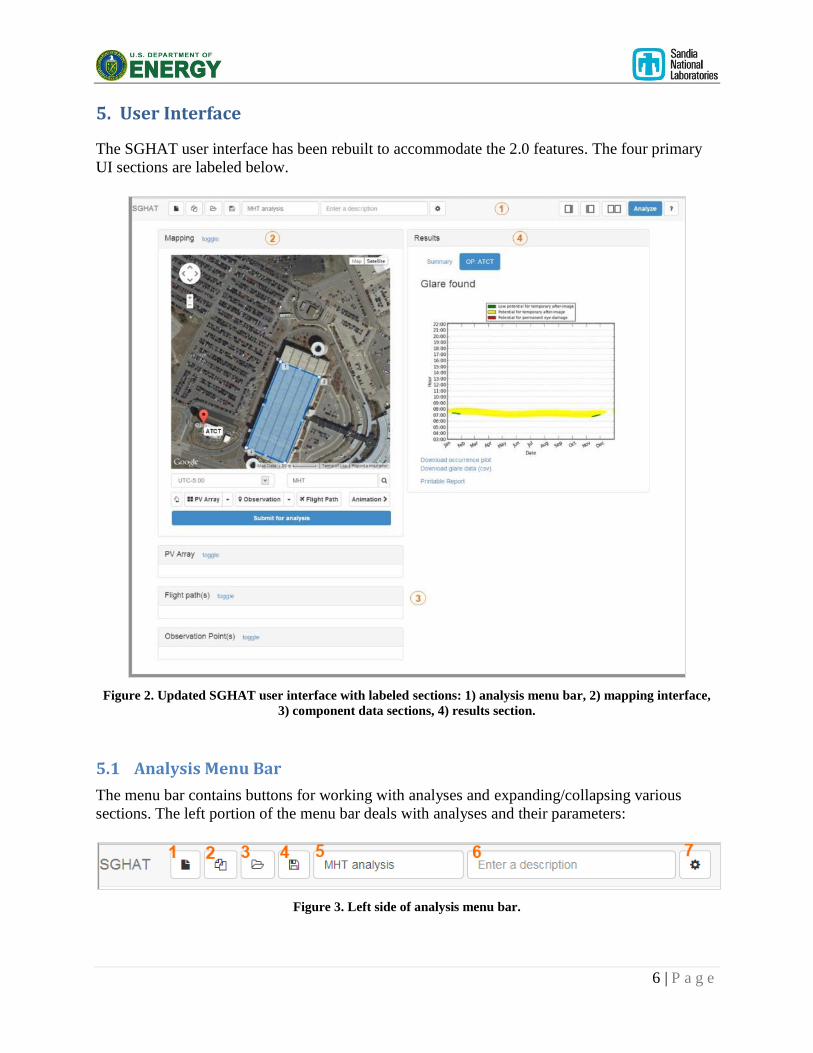
The SGHAT user interface has been rebuilt to accommodate the 2.0 features. The four primary

UI sections are labeled below.

Figure 2. Updated SGHAT user interface with labeled sections: 1) analysis menu bar, 2) mapping interface,

3) component data sections, 4) results section.

5.1 Analysis Menu Bar

The menu bar contains buttons for working with analyses and expanding/collapsing various

sections. The left portion of the menu bar deals with analyses and their parameters:

Figure 3. Left side of analysis menu bar.

7 | P a g e

1. New Analysis

Brings up the New Analysis screen where the user can enter a name and select a timezone to

create a new analysis. The previous analysis will be saved.

2. Clone Analysis

Create a new analysis and populate it with the components (PV array, observation points, flight

paths) of the current analysis. This is similar to the common “Save As…” functionality.

3. Load Analysis

Display a list of previously-saved analyses. Select an analysis to load it, or click “delete” to

permanently delete it.

4. Save

Save the current analysis and components. Note that analyses and components are auto-saved

when changed.

5. Analysis name

Modify the name of the current analysis. The name must be unique.

6. Analysis description

An optional description can be entered. The description does not have to be unique.

7. Analysis configuration

Display the analysis configuration screen. Use this to change parameters such as the time

interval, height units, etc. See Appendix A for detailed descriptions of each parameter.

The right portion of the menu bar has the following buttons:

Figure 4. Right side of analysis menu bar.

1. Expand Map and Component sections

Expand the left sections (mapping and components). The Results section on the right is

minimized.

2. Expand Results section

Expand the Results section to fill the screen. The mapping and component sections are

minimized.

3. Restore Both

All sections are restored to their original sizes and take up 50% of the screen.

8 | P a g e

4. Analyze

Submit the current analysis for processing. A glare analysis will be performed based on the

analysis parameters and drawn components (PV array, observation point(s) and/or flight path(s)).

5. View Help

Display the Help screen which provides a quick-start guide and links to relevant resources.

5.2 Google Map Section and Controls

The mapping sections contains buttons for adding map components, running glare animations

and setting the analysis time zone. In brief, components are added by clicking on the respective

button and then clicking on the map to set the location of the component.

Observation points and the PV array can be removed by right-clicking them on the map when in

Select mode, or by clicking the “Remove” button in their data section. Flight paths can be

removed by clicking the “Remove” button or by clicking on the threshold point and selecting

“Remove”.

Figure 5. Map and drawing controls for adding analysis components.

1. Select time zone

Select the standard time zone offset of the location being analyzed. Options are UTC-12 through

UTC+14.

2. Map search

Enter a location to center the Google Map. This functions exactly like the actual Google Map

search. Note that analysis components are not affected when the map location changes.

3. Select Tool

Activate the Map Select Mode to manually pan the map or move the position of PV array

vertices and observation points. Note that flight path observation points can only be adjusted by

changing the flight path direction.

4. PV Array Tool

Activate the PV array drawing mode to draw an array on the map. The default mode uses click-

and-drag to draw a rectangular PV array. Use the drop-down menu to select Polygonal mode in

order to click and set each array vertex manually.

9 | P a g e

5. Observation Point Tool

Activate the Observation Point drawing mode. Click on the map to add a new observation point.

SGHAT automatically queries Google for the ground elevation of the point. Using the dropdown

menu, select the ATCT Point mode to automatically set the observation point label to ‘ATCT’.

6. Flight Path Tool

Activate the flight path drawing mode. Click once on the map to set the runway threshold point.

Click again to specify the flight path direction. Eight observation points will be added in this

direction, spaced at quarter-mile intervals on the map.

7. Animation Menu

Click to open the Animation Menu:

Figure 6. Animation controls.

In the menu, select a date, PV array and observation point and click the Play button to view the

location of glare along the PV array surface for the given day, as it changes over time. The

Backwards and Forwards buttons can be used to manually step through the times of glare.

8. Submit Analysis

Submit the analysis parameters and components for glare analysis. The results will appear in the

Results section once the analysis is complete.

5.3 Component Data Sections

There are three component types: PV array, flight path and observation point. When drawn on

the map, the properties of each component are displayed in a respective component section for

convenient editing.

10 | P a g e

PV Array Section

The PV array section displays the configurable parameters of the PV array and its vertices

(corners).

Figure 7. Sample data section of PV array, including table of vertex (corner) coordinates.

See Appendix B for detailed descriptions of each parameter.

Note that the vertex coordinates, including elevation, are independent of the orientation and tilt.

The vertices establish the tilt of the PV-array plane and do not influence the tilt or orientation of

the individual panels themselves. For example, panels mounted flush on a 30° pitched roof will

have PV-array vertices with different elevations to accommodate the pitched roof and resulting

tilted PV-array plane (e.g., two vertices at 15 feet and two vertices at 10 feet). However, the

panels should still be prescribed with a tilt of 30° (if they are flush mounted against the 30°

pitched roof) and the appropriate orientation. A tilt of 0° indicates that the panels are parallel

with the earth’s surface and facing upward, regardless of the prescribed vertex elevations.

The array vertex parameters are all editable – entering a new latitude or longitude will

automatically adjust the corresponding vertex on the map. Values for vertex heights above

ground must be entered before a glare analysis can be performed.

Flight Path Section

The flight path section contains entries for each flight path added on the map. Each entry

displays the configurable parameters of the flight path as well as observation points. In addition,

11 | P a g e

the user can choose to limit the downward and azimuthal angles of view from the flight path

observation points to simulate restricted viewing from the cockpit by checking “Consider pilot

visibility from cockpit.” If checked, the default maximum downward viewing angle is set to 30

degrees and the default azimuthal viewing angle is set to 180 degrees, both of which can be

modified [3]. See Appendix C. Note that a glide slope of 3 degrees conforms to the Federal

Aviation Administration guidelines for analyzing flight paths (78 FR 63276).

Figure 8. Sample data section of flight path, including table of observation point coordinates.

Observation Point Section

Non-flight-path observation points are displayed in a tabular format in their data section:

12 | P a g e

Figure 9. Observation point data section with two sample observation points.

Observation points are fully editable. Changes to the name, latitude or longitude of an

observation point will be reflected on the map.

5.4 Results Section

Glare analysis results for each PV array are displayed in the Results section on the right side of

the SGHAT page.

Figure 10. Results section summary tab, with overview table of glare found.

13 | P a g e

A table summarizes the resulting glare for each flight path and observation point. Links on the

top of the results section can be used to navigate to specific results.

Observation Point Results

Observation points that experience glare will show results similar to the following figure:

Figure 11. Results tab for observation point (ATCT), with glare occurrence plot.

The Observation Point (“OP”) result shows the glare occurrence plot. Below it are links for

generating a printable report and for downloading the plot and glare data in comma-separated

format. Finally, a glare hazard plot can be created for a selected day using the controls at the

bottom. The following figure is an example hazard plot:

14 | P a g e

Figure 12. Glare hazard plot showing glare with potential to cause temporary after-image at several times

during the course of a day.

Flight Path Results

Flight path results contain data for glare found at each observation point (OP) comprising the

flight path. Results for each OP are contained in expandable tabs. By clicking on the OP name

the results section will expand to display results in the same format as solo OP results, with a

glare occurrence plot and links for generating a printable report or downloading data.

Finally, a link to generate a printable flight path report can be used to print a summary of the

entire flight path analysis.

15 | P a g e

Figure 13. Results tab for flight path with OP results contained in expandable sections.

16 | P a g e

Sample Glare Occurrence Plot

The Glare Occurrence Plot shows when glare can occur (as viewed from the prescribed

observation point) throughout the year. The color of the dots indicates the potential ocular

hazard [1] as shown in Figure 14. In the example shown in Figure 14, glare is predicted to be

visible from the prescribed observation point during the morning from January to November for

~30 – 40 minutes. The color of the plotted points indicates the potential ocular hazard. In Figure

14, the yellow dots indicate that the glare in this particular example has the potential to cause a

temporary after-image.

Figure 14. Glare occurrence plot showing when glare can occur (time and date) and the potential for ocular

impact (represented by the color of the dots). Times are shown in Standard Time (during Daylight Savings

Time, add one hour).

Note that for flight path observation points, yellow glare beyond 50º azimuthally from the line of

sight of the pilot is reduced to transparent green glare. This downgrading is due to recent

research which found that the ocular impact is reduced when glare is outside the line of sight.

Points that were originally in the “green” (low potential for temporary after-image) or “red”

(potential for permanent eye damage) are not changed.

17 | P a g e

Figure 15. Before (left) and after (right) the algorithm update which treats yellow glare 50º beyond the pilot

line-of-sight as transparent green. The majority of detected yellow glare in this sample was beyond this 50º

range.

18 | P a g e

6. Case Study and Example

We include a sample analysis of the Manchester-Boston Regional Airport (MHT), which has

experienced glare from PV panels that were installed on the roof of a parking garage near the air

traffic control tower. The blue highlighted area in Figure 16 is drawn by the user to denote the

location of the PV array. The red marker indicates the location of the observer in the air traffic

control tower.

Figure 16. Screen image of glare analysis of the Manchester Boston Regional Airport. PV array (blue

outline) and observation point (red marker) are entered using drawing tools integrated with Google Maps.

6.1 ATCT analysis

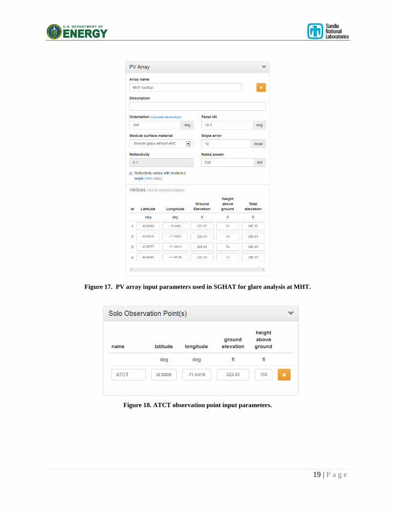
Figure 17 through Figure 19 show other input parameters entered by the user, including

orientation and tilt of the PV array, elevations, rated power (for energy production calculations),

optical and ocular parameters. The latitude, longitude, and elevation coordinates of the user-

drawn PV array and observation points are automatically calculated in Google Maps and used to

determine sun position and vector calculations for the glare and energy production analyses.

19 | P a g e

Figure 17. PV array input parameters used in SGHAT for glare analysis at MHT.

Figure 18. ATCT observation point input parameters.

20 | P a g e

Figure 19. Analysis configuration parameters for MHT analysis.

Figure 20 and Figure 22 show the results of the glare analysis assuming different values for the

optical slope error of the PV modules, which impacts the scatter and beam spread. The dots in

the plot represent occurrences of glare as viewed from the user-specified observation point

relative to the specified PV array as a function of the time of day and day of the year. The color

of the dots indicates the potential ocular hazard, which is impacted by the direct normal

irradiance, optical parameters (reflectance, slope error/scatter), and ocular parameters (pupil

diameter, transmission coefficient, ocular focal length). In Figure 20 and Figure 22, there is a

potential for glare that can cause temporary after-image (a lingering image of the glare in the

field of view) during the early morning for most months of the year Assuming an optical slope

error of 10 mrad, which yields a total beam spread of the reflected glare image of 0.13 rad (~7

degrees), predicts that glare will be visible for more days throughout the year and for a slightly

longer period each day when compared to the results using a slope error of 0 mrad, which has

less scatter and beam spreading (0.0093 rad or ~0.5 degrees).

At MHT, the general spatial and temporal pattern of glare is shown in Figure 23.

21 | P a g e

Figure 20. Results section and plot showing when glare can occur (time and date) and the potential for ocular

impact (represented by the color of the dots) in the ATCT assuming an elevation of 150 ft above ground level

with an optical slope error of 10 mrad (total beam spread of 0.1293 rad). Times are Eastern Standard Time

(during Daylight Savings Time, add one hour).

22 | P a g e

Figure 21. Hazard plot denoting visual impact of glare predicted for June 5. Glare has the potential to cause

temporary after-image.

23 | P a g e

Figure 22. Glare occurrence plot for MHT ATCT with slope error of 0, yielding total beam spread of 9.3

mrad (the subtended angle of the sun).

Figure 23. Approximate predicted locations and movement of glare on PV array at various times of the year.

Photos and videos of glare from the installed PV array at MHT were taken from the Air Traffic

Control Tower in late April and early May. Glare was observed during hours that were

consistent with those predicted by the glare tool (see Figure 24 and Figure 25; note that the

hours shown in the ocular hazard plot in Figure 20 and Figure 22 are Eastern Standard Time, but

the times shown in the photos in Figure 24 and Figure 25 are Eastern Daylight Time). Because

of the glare, tarp was placed over the offending PV modules.

~June

~March, September

~December

24 | P a g e

Features such as gaps between modules, uncertainty in the relative height of the PV modules and

observation points, obstructions/land features between the PV array and the observation point,

uncertainty in the optical properties of the modules, and atmospheric attenuation may impact the

actual perception and time of observed glare.

Figure 24. Glare viewed from Air Traffic Control Tower at Manchester/Boston Regional Airport

(8:15 AM EDT, 4/27/12).

25 | P a g e

Figure 25. Glare viewed from Air Traffic Control Tower at Manchester/Boston Regional Airport (~8:17 AM

EDT, 5/10/12). Note that tarp has been placed over some of the modules.

6.2 Energy optimization

The Solar Glare Hazard Analysis Tool can also be used to predict the relative energy production

from alternative configurations (orientation, tilt, etc.) so that designs can be identified that not

only mitigate glare but also maximize energy production. Table 1 shows alternative

configurations using the same footprint of the PV array shown in Figure 16 that are predicted to

produce no glare. The relative annual energy production is also shown for each configuration.

In addition, the current PV configuration (200° azimuthal angle, 20.6° elevation angle) and a

maximum energy production configuration (180° azimuthal angle, 43° elevation angle) are

shown in Table 1. The optimal configuration using the same footprint that is predicted to

produce no glare to the ATCT while maximizing energy production employs an azimuthal angle

of 120° and an elevation angle of 40°.

26 | P a g e

Table 1. Alternative PV array configurations that are predicted to produce no glare to the ATCT (unless

otherwise noted). Azimuthal angle is measured clockwise from due north (0°); elevation angle is measured

from 0° (facing up) to 90° (facing horizontal). Note: these analyses assumed an ATCT cabin elevation of 51.2

m. We were informed later that the cabin elevation was lower (~45 m), so other configurations with no glare

to the ATCT are possible (e.g., Az=110°, El=20.6°).

Azimuthal Angle (degrees)

Elevation Angle (degrees)

Relative Annual Energy Production

180 43 100.0%*

200 20.6 93.9%**

120 40 88.9%

120 50 87.2%

110 30 85.0%

110 40 84.7%

120 60 83.7%

110 50 82.8%

130 70 81.5%

100 30 80.9%

100 20 80.8%

100 40 79.9%

110 60 79.3%

120 70 78.3%

100 50 77.6%

90 20 77.5%

210 80 76.9%

90 30 76.4%

220 80 75.8%

90 40 74.5%

110 70 74.2%

100 60 74.1%

130 80 74.0%

90 50 71.8%

120 80 71.3%

100 70 69.2%

90 60 68.1%

110 80 67.7%

90 70 63.4%

100 80 63.2%

90 80 57.8% *Maximum energy production; produces glare to ATCT

**Current configuration; produces glare to ATCT

Based on a review of the glare analyses, an alternative configuration of the PV modules was

recommended where the assemblies are rotated 90° counter-clockwise so that they are facing

27 | P a g e

toward the east-southeast (110° from due north). The tilt of the modules remains the same

(however, since the downward tilt of the roof is 1.2° from east to west, the actual tilt of the

modules is 20.7° - 1.2° = 19.5°.

Figure 26 shows a screen image of the SGHAT analysis with the PV array outlined in blue and

the location of the ATCT indicated by the red marker.

Figure 26. Location of alternative PV array configuration (outlined in blue) rotated 90° counter-clockwise so

that they are facing toward the east-southeast (110° from due north).

6.3 Flight path analysis

In addition to the ATCT, observation points along straight approaches to runways 35, 6, 17, 24

were also evaluated assuming a glide slope of 3 degrees. The distance legend on the Google map

is used (along with a ruler) to specify observation points and desired distances from the

touchdown point on the landing strip. See Table 2 and Figure 27 – Figure 30 for locations and

elevations of observation points along the approach to these runways.

For this new configuration (PV assemblies rotated 90° counter-clockwise as shown in Figure

26), no glare was predicted to be observed in the ATCT or at the observation points along the

approaches to runways 35, 6, and 17. It should be noted that the elevation of the ATCT

observation point was varied between 40 – 51 m and no glare was predicted. Based on drawings

of the ATCT tower, the elevation of the ATCT cabin is ~45 m.

The annual energy produced from this new configuration was predicted to be within ~1% of the

existing configuration. The existing configuration consists of 2210 modules with a rated power

capacity of ~530 kW (~240 W/module). The new configuration has 247 additional modules for

28 | P a g e

a rated power capacity of ~589 kW. Using these values, SGHAT predicts that the maximum

annual energy production for the existing and new designs are 1.04 GWh and 1.16 GWh,

respectively, assuming clear-sky conditions. Actual annual energy production will be less due to

variable (lower) DNI when the sky is cloudy.

Table 2. Observation points for approaches to runways 35, 6, 17, and 24 assuming a 3 degree glide slope.

Observation

Point

Height above

ground (ft)

Threshold 52

¼ mile 121

½ mi. 190

¾ mi. 259

1 mi. 328

1 ¼ mi. 397

1 ½ mi. 467

1 ¾ mi. 536

2 mi. 605

Figure 27. Observation points approaching Runway 35 from the southeast.

29 | P a g e

Figure 28. Observation points approaching Runway 6 from the southwest.

Figure 29. Observation points approaching Runway 17 from the northwest.

30 | P a g e

Figure 30. Observation points approaching Runway 24 from the northeast.

7. Acknowledgments

Sandia National Laboratories is a multi-program laboratory managed and operated by Sandia

Corporation, a wholly owned subsidiary of Lockheed Martin Corporation, for the U.S.

Department of Energy’s National Nuclear Security Administration under contract DE-AC04-

94AL85000.

8. References

[1] Ho, C.K., C.M. Ghanbari, and R.B. Diver, 2011, Methodology to Assess Potential Glint

and Glare Hazards From Concentrating Solar Power Plants: Analytical Models and

Experimental Validation, Journal of Solar Energy Engineering-Transactions of the Asme,

133(3).

[2] Duffie, J.A. and W.A. Beckman, 1991, Solar engineering of thermal processes, 2nd ed.,

Wiley, New York, xxiii, 919 p.

[3] Federal Aviation Administration Advisory Circular, 1993, Pilot Compartment View

Design Considerations, AC No: 25.773-1, U.S. Department of Transportation, January 8,

1993.

[4] Sliney, D.H. and B.C. Freasier, 1973, Evaluation of Optical Radiation Hazards, Applied

Optics, 12(1), p. 1-24.

Additional references can be found at www.sandia.gov/glare.

31 | P a g e

Appendix A – Analysis Parameters

Height Units: Select the units of distance for the height of solar panels and the height

above ground of each observation point in feet or meters.

Subtended angle of the sun: The average subtended angle of the sun as viewed from

earth is ~9.3 mrad or 0.5°.

Peak DNI: The maximum Direct Normal Irradiance (W/m2) at the given location at solar

noon. This value may be scaled at each time step to account for the changing position of

the sun and reduced DNI in the mornings and evenings if the “variable” option is selected

in the next field. On a clear sunny day at solar noon, a typical peak DNI is ~1,000 W/m2.

DNI variability: “Variable” scales the peak DNI at each time step based on the changing

position of the sun. “Fixed” uses the peak DNI value for every time step throughout the

analysis, with no scaling.

Ocular transmission coefficient: The ocular transmission coefficient accounts for

radiation that is absorbed in the eye before reaching the retina. A value of 0.5 is typical

[1, 4].

Pupil diameter: Diameter of the pupil (m). The size impacts the amount of light

entering the eye and reaching the retina. Typical values range from 0.002 m for daylight-

adjusted eyes to 0.008 m for nighttime vision [1, 4].

Eye focal length: Distance between the nodal point (where rays intersect in the eye) and

the retina. This value is used to determine the projected image size on the retina for a

given subtended angle of the glare source. Typical value is 0.017 m [1, 4].

Time interval: Specify the time step for the glare analysis. The sun position will be

determined at each time step throughout the year. A time step of 1 minute yields

excellent resolution.

Appendix B – PV Array Parameters

Axis tracking: Indicate the type of tracking used by the panels (if any). “None” for

fixed-tilt panels, “single” for single-axis tracking and “dual” for dual-axis tracking. Note

that tracking affects the positioning of the panels at every time step while the sun is up.

o Orientation of array: (fixed-tilt panels) Specify the orientation of the array in

degrees, measured clockwise from true north. Modules facing east would have an

orientation of 90°, and modules facing south would have an orientation of 180°.

The “Calculate declination” link can be used to determine the orientation if an

angle based on magnetic north is known.

o Tilt of solar panels: (fixed-tilt panels) Specify the tilt (elevation angle) of the

modules in degrees, where 0° is facing up and 90° is facing horizontally.

o Tilt of tracking axis: (single-axis tracking) Specify the elevation angle of the

tracking axis in degrees, where 0° is facing up and 90° is facing horizontally. The

panels rotate about the tracking axis.

32 | P a g e

o Orientation of tracking axis: (single-axis tracking). Specify the orientation of the

tracking axis in degrees, measured clockwise from true north. Panels facing south

at solar noon would have an orientation of 180°. Panels facing east at solar noon

would have an orientation of 90°. Note: if the tilt of the tracking axis is 0°, an

orientation of the tracking axis of either 0° or 180° yields the same results.

o Offset angle of module: (single-axis tracking). Specify, in degrees, the vertical

offset angle between the tracking axis and the panel (if any). See Figure 4.6 in

http://www.powerfromthesun.net/Book/chapter04/chapter04.html#4.1.2%20Singl

e-Axis%20Tracking%20Apertures.

o Limit the rotation angle: (single-axis tracking). If checked, a maximum angle of

rotation will be used to constrain the tracking rotation in both clockwise and

counterclockwise directions.

Maximum tracking angle: (single-axis tracking). The maximum angle the

panel will rotate in both the clockwise and counterclockwise directions

from the zenith (upward) position.

Rated power: Specify the rated power (kW) of the PV system. This is used to calculate

the maximum annual energy produced (kWh) from the system in the prescribed

configuration (assuming clear sunny days). This is useful for comparing alternative

configurations to determine which one has the maximum energy production.

Module surface material: specify the type of material comprising the PV modules. The

reflectivities of the material choices have been characterized in order to generate scaled

values for each time step.

Correlate slope error to module surface type. If checked, the slope error value will be set

according to the following table, based on the selected material:

Table 3. Slope error and beam spread vs. surface type

PV Glass Cover Type Average

RMS Slope Error (mrad)

Average Beam

Spread (mrad)

Standard deviation of slope error

Standard deviation of beam error

Smooth Glass without Anti-Reflection Coating

6.55 87.9 4.43 53.3

Smooth Glass with Anti-Reflection Coating

8.43 110 2.58 30.9

Light Textured Glass without Anti-Reflection

Coating 9.70 126 2.78 33.3

Light Textured Glass with Anti-Reflection Coating

9.16 119 3.17 38.0

Deeply Textured Glass 82.6 1000 N/A N/A

o Slope error: specifies the amount of scatter that occurs from the PV module.

Mirror-like surfaces that produce specular reflections will have a slope error

closer to zero, while rough surfaces that produce more scattered (diffuse)

reflections have higher slope errors. Based on observed glare from different PV

modules, an RMS slope error of ~10 mrad (which produces a total reflected beam

33 | P a g e

spread of 0.13 rad or 7°) appears to be a reasonable value. Not used if correlate

slope error to module surface type is checked.

Reflectivity varies with incidence angle: If checked, the reflectivity of the modules at

each time step will be calculated as a function of module surface material and incidence

angle between the panel normal and sun position (see Appendix E).

o

o Reflectivity of PV module: Specify the solar reflectance of the PV module.

Although near-normal specular reflectance of PV glass (e.g., with antireflective

coating) can be as low as ~1-2%, the reflectance can increase as the incidence

angle of the sunlight increases (glancing angles). Based on evaluation of several

different PV modules, an average reflectance of 10% is entered as a default value.

Only used if reflectivity does not vary with incidence angle.

The following list comprises the array vertex parameters:

Latitude: geographic coordinate, in degrees, representing north-south position of the

point. 0 at the equator and positive above it.

Longitude: geographic coordinate, in degrees, representing east-west position of the

point. The value must be between -180 and 180, with 0 at the Prime Meridian and

negative to the west of it.

Ground Elevation: the height above sea level of the ground at the position of the point.

Height above ground: The absolute height of the observation point above the ground

elevation.

Total elevation: the sum of the ground elevation and height above ground. Changes to

this value are automatically reflected in the “height above ground” input. Use this if, for

example, the PV array sits on a roof and the height of a building is known. Enter the

height in the “total elevation” field and the heights above ground for each array vertex

will be automatically determined.

Appendix C –Flight Path Parameters

direction: angle, in degrees, from threshold along which to specify observations. 0 is true

north, 90 is due east of true north. Note that the direction value may deviate from the

specified runway angle.

threshold crossing height: height above ground of aircraft as it crosses threshold point.

glide slope: angle, in degrees, of ascent/descent of aircraft along path. Defaults to 3°.

consider pilot visibility from cockpit: If checked, glare below the “max downward

viewing angle” is ignored. Defaults to unchecked.

o max downward viewing angle: The angle below the horizon indicating the field

of view of the pilot in the cockpit from the flight path observation points. Glare

34 | P a g e

occurring below this field of view is ignored. Only used if “consider pilot

visibility from cockpit” is checked. Defaults to 30°.

o Azimuthal viewing angle: The horizontal angle clockwise and counter-clockwise

from the front of the aircraft parallel with the horizon. Glare occurring past this

field of view is ignored. An azimuthal viewing angle of 180° means glare behind

the aircraft can be seen (360° field of view). Default value is set to 180°.

For flight path observation point parameters, see Appendix D.

Appendix D – Observation Point Parameters

Latitude: geographic coordinate, in degrees, representing north-south position of the

point. 0 at the equator and positive above it.

Longitude: geographic coordinate, in degrees, representing east-west position of the

point. The value must be between -180 and 180, with 0 at the Prime Meridian and

negative to the west of it.

Ground Elevation: the height above sea level of the ground at the position of the point.

Height above ground: The absolute height of the observation point above the ground

elevation.

Appendix E – Reflectance vs. Incidence Angle

The reflectance of the module surfaces is highly dependent on the incidence angle of the sunlight

relative to the surface normal. In general, the reflectance of glass is relatively low (< 5%) at

small incidence angles but increases rapidly above 60°. Higher reflectances increase the glare

intensity, retinal irradiance, and potential for ocular impact. Figure 31 displays measured

reflectances vs. incidence angle for various PV module materials measured by Sandia National

Laboratories.

35 | P a g e

Nomenclature for labeling: “AR_glass-texturing_cell-type_backsheet-color_frame-color_power-rating”

a. AR: Anti-reflective coating was present b. Glass-texturing: smooth (none), light, or deep c. Cell-type: monocyrstalline or polycrystalline d. Backsheet-color: white or black e. Frame-color: silver or black f. Power-rating: power rating in Watts

Figure 31. Measured reflectance vs. incidence angle for different PV surface materials.

The data sets were grouped into similar categories (e.g., roughness, coating), and polynomial

regressions were applied to these data sets to determine approximate reflectance values as a

function of incidence angle for five PV glass cover types: (1) smooth glass without anti-

reflection coating, (2) smooth glass with anti-reflection coating, (3) lightly textured glass without

anti-reflection coating, (4) lightly textured glass with anti-reflection coating, and (5) deeply

textured glass. Profilometry tests revealed that the lightly textured glass had an average surface

roughness of ~1 – 2 microns, and the deeply textured glass had an average surface roughness of

~17 microns. contains the curve fits for each material type. These functions are used by

SGHAT when determining the reflectance of the PV array panels as a function of the incidence

angle of the incoming sunlight at each time step.

36 | P a g e

Table 4. Piece-wise functions describing the reflectance curves of the different types of PV glass covers.

Angle, , is the incidence angle. In the fit functions, ‘y’ is the reflectance and ‘x’ is the angle of incidence.

PV Glass Cover Type Fit Function Defined over 0 60

Fit Function Defined over

60 < < 90 Smooth Glass without Anti-Reflection Coating

y = 1.1977E-5 x2 – 9.5728E-4 x + 4.410E-2 y = 6.2952E-5 e

0.1019x

Smooth Glass with Anti-Reflection Coating

y = 1.473E-5 x2 – 9.6416E-4 x + 3.2395E-2 y = 4.7464E-5 e

0.1051x

Light Textured Glass without Anti-Reflection Coating

y = 1.5272E-5 x2 – 1.1304E-3 x + 4.305E-2 y = 7.3804E-5 e

0.0994x

Light Textured Glass with Anti-Reflection Coating

y = 1.4188E-5 x2 – 1.0326E-3 x + 3.9016E-2 y = 7.0179E-5 e

0.0994x

Deeply Textured Glass y = 6.8750E-6 x2 – 6.5250E-4 x + 2.10E-2 y = 4.1793E-5 e

0.0834x