solar augmentation of process steam oilers for ogeneration
TRANSCRIPT

Solar Augmentation of Process Steam Boilers for Cogeneration
Prepared by:
Onekai Adeliade Rwezuva
RWZONE001
Department of Mechanical Engineering
University of Cape Town
Supervisor:
A/Prof. Wim Fuls
December 2020
Submitted to the Department of Mechanical Engineering at the University of Cape Town in partial
fulfilment of the academic requirements for a Master of Science degree in Mechanical Engineering
Key Words: Solar assisted power generation, Heat exchanger sizing
Universi
ty of
Cape T
own

The copyright of this thesis vests in the author. No quotation from it or information derived from it is to be published without full acknowledgement of the source. The thesis is to be used for private study or non-commercial research purposes only.
Published by the University of Cape Town (UCT) in terms of the non-exclusive license granted to UCT by the author.
Universi
ty of
Cape T
own

i
Abstract
In this study, the techno-economic feasibility of converting an existing process steam plant into a
combined heat and power plant, using an external solar thermal field as the additional heat source
was studied. Technical feasibility entailed designing a suitable heat exchanger, which uses hot oil
from the solar field to raise the steam conditions from dry saturated to superheated. The solar field
was sized to heat a selected heat transfer fluid to its maximum attainable temperature. A suitable
turbine-alternator was chosen which can meet the required plant power demand. For this to be a
success, the processes which require process steam were analysed and a MathCAD model was
created to design the heat exchanger and check turbine output using the equations adapted from
various thermodynamics and power plant engineering texts, together with the Standards for the
Tubular Exchanger Manufacturer’s Association. The U.S. National Renewable Energy Laboratory
system advisor model was used to size the suitable solar field.
A financial model was developed in Excel to check the economic feasibility of the project, using
discounted payback period as the economic indicator. It was found out that amongst loan interest
rates, variation of system output and the electricity output, the profitability of the project was
largely influenced by the electricity tariff. An optimum size for the heat exchanger of 30ft was
established from the sensitivity analysis and it was concluded that the project is currently not
economically viable on an independent investor financing model, unless either the electricity tariff
improves or the solar thermal energy and turbine technology costs decrease.

ii
Declaration
I, Onekai Adeliade Rwezuva, hereby declare the work contained in this dissertation to be my own.
All information that has been gained from various journal articles, textbooks or other sources has
been referenced accordingly. I have not allowed and will not allow anyone to copy my work to pass
it off as their own work or part thereof.
________________________ __________________________
Name Date 05/03/2021Onekai A Rwezuva

iii
Acknowledgements
To my parents, for being my pillar of strength and believing in me. Thank you…
Firstly, I would like to thank my supervisor A/Prof. Wim Fuls whose assistance in my research I
cannot put a price tag on. It was not an easy journey but your emphasis on going down to
fundamentals and in-depth knowledge in power plant systems has been a unique resource I could
not do without. I am very grateful.
Secondly, I very much acknowledge Prof. T. Harms from the Solar Thermal Energy Research Group
from the University of Stellenbosch for his assistance in the solar design aspect of my research. You
came through and answered my questions like I was part of the STERG family. I appreciate.
I would also like to thank the Mandela Rhodes Foundation for financing my studies and I hope I will
take with me the vision of the foundation and put my education to good use for the betterment of
the continent.
Many thanks go to the staff at John Thompson Boilers, Tongaat Hulett Triangle, African Distillers and
Kadoma Paper Mills for providing the vital information which formed the basis of this study. Special
mention goes to my friends and family who have always been supportive of my endeavours, and
the postgraduate community at the University of Cape Town, particularly the AtPROM research unit.
You made it bearable to be in a new environment, thank you.
Above all, I thank the Lord Almighty for his guidance and grace. Most certainly, the skills I acquired
whilst working on this research will help me grow, both personally and professionally.
iv
Table of Contents
List of Figures ...................................................................................................................................... vi
List of Tables ...................................................................................................................................... viii
List of Nomenclature ........................................................................................................................... ix
1. Introduction .................................................................................................................................. 1
1.1 Background to the problem .................................................................................................. 1
1.2 Project aim ............................................................................................................................ 1
1.3 Project scope and limitation ................................................................................................. 2
1.4 Research outline .................................................................................................................... 3
1.5 Expected outcomes ............................................................................................................... 4
1.6 Disclaimer .............................................................................................................................. 4
2. Literature Review .......................................................................................................................... 5
2.1 Process steam plant and the Rankine cycle .......................................................................... 5
2.2 Cogeneration ......................................................................................................................... 7
2.3 Solar thermal systems ........................................................................................................... 9
2.4 Heat exchanger design ........................................................................................................ 13
2.5 Shell and tube-side pressure drops ..................................................................................... 32
2.6 Feedwater heater structural design .................................................................................... 33
2.7 Steam turbines and application to small steam plants ....................................................... 33
2.8 Steam plant economics ....................................................................................................... 40
2.9 Conclusion ........................................................................................................................... 44
3. Methodology ............................................................................................................................... 45
3.1 Model Investigation............................................................................................................. 45
3.2 Site visit reports ................................................................................................................... 46
3.3 Model development ............................................................................................................ 51
4. Results and Discussion ................................................................................................................ 70
4.1 System Model ...................................................................................................................... 70
4.2 Physical system parameters ................................................................................................ 71
4.3 Energy output ...................................................................................................................... 72
4.4 System outputs .................................................................................................................... 78
v
4.5 Performance Evaluation ...................................................................................................... 79
4.6 System capital costs ............................................................................................................ 81
4.7 Payback period and optimal length .................................................................................... 83
4.8 Sensitivity Analysis .............................................................................................................. 84
5. Conclusions and Recommendations ........................................................................................... 89
5.1 Conclusion…………………………………. ....................................................................................... 89
5.2 Recommendations .............................................................................................................. 90
6. Bibliography ................................................................................................................................ 92
Appendix A. Heat exchanger approximate sizing ......................................................................... 96
Appendix B. Heat exchanger program code ................................................................................. 98
Appendix C. Turbine calculations program code ........................................................................ 116
Appendix D. Turbine Quote ........................................................................................................ 118

vi
List of Figures
Fig 1: Research Outline flow diagram .................................................................................................. 3
Figure 2: Rankine cycle basic flow diagram ......................................................................................... 5
Figure 3: Ideal Rankine cycle T-s diagram ............................................................................................ 6
Figure 4: Cogeneration – Back Pressure Steam turbine topping cycle ................................................ 8
Figure 5: Solar thermal system basic layout ........................................................................................ 9
Figure 6: Cameo Generating Station SAPG system [15] .................................................................... 11
Figure 7: Concentrated Solar Power Parabolic Trough system adapted from the US Department of
Energy [18] ......................................................................................................................................... 12
Figure 8: Shell and Tube Heat Exchanger layout ............................................................................... 14
Figure 9: Heat Exchanger Schematic .................................................................................................. 14
Figure 10:Temperature differences for different heat exchanger flow arrangements..................... 15
Figure 11:TEMA Exchanger types adapted from Standards of the Tubular Exchanger Manufacturers
Association, 9th Edition [21] .............................................................................................................. 20
Figure 12: Baffle and tube bundle geometries [32] ........................................................................... 26
Figure 13:Tube layouts adapted from NPTEL Chemical Engineering Design Module I [33] .............. 27
Figure 14: Single segmental shell and tube type E shell showing baffle spacings [32] ..................... 29
Figure 15: Shell-side flow paths in a segmental baffled heat exchanger [32] ................................... 30
Figure 16: Shell & Tube heat exchanger design flow chart adapted from Heat Exchanger Design
Handbook [23] ................................................................................................................................... 32
Figure 17: Typical turbine condition line ........................................................................................... 37
Figure 18: Siemens SST-060 Turbo-alternator set ............................................................................. 39
Figure 19: SST-060 Specifications [39] ............................................................................................... 40
Figure 20: Tongaat Hulett Triangle Process Flow Diagram ................................................................ 48
Figure 21: Tongaat Hulett Triangle Steam & Condensate Flow Diagram .......................................... 49
Figure 22: Solar thermal feedwater heating and boiler modification for superheating .................. 52
Figure 23: Direct solar integration for superheating ......................................................................... 53

vii
Figure 24: Indirect solar thermal integration with superheat ........................................................... 54
Figure 25: Indirect solar thermal integration with superheat and feedwater heating ..................... 55
Figure 26: AFDIS GHI and dry bulb temperature annual variations from SAM NREL ........................ 56
Figure 27: Heat exchanger approximate design flow chart [23] ....................................................... 59
Figure 28: Solar field system design inputs ....................................................................................... 66
Figure 29: Proposed steam plant process flow diagram ................................................................... 70
Figure 30: Steam heat addition vs heat exchanger length ................................................................ 72
Figure 31: Timestep- averaged system outlet temperature .............................................................. 73
Figure 32: Typical daily hourly average thermal energy variation per month for a 1.06 MW (base
case) design heat sink power ............................................................................................................. 74
Figure 33: Annual daily hourly average output required for solar output throughout the year. ..... 75
Figure 34: Annual thermal energy output for normal solar field ...................................................... 76
Figure 35: Variation of heat exchanger effectiveness and imported power with the heat exchanger
length ................................................................................................................................................. 79
Figure 36: System capital costs breakdown ....................................................................................... 82
Figure 37: Total investment required and payback period vs heat exchanger length for normal solar
output ................................................................................................................................................. 83
Figure 38: : Total investment required and payback period vs heat exchanger length for maximum
solar output ........................................................................................................................................ 84

viii
List of Tables
Table 1: Kadoma Paper Mills Process Steam Requirements ............................................................. 47
Table 2: African Distillers Process Steam Requirements ................................................................... 51
Table 3: System Boundary Conditions ............................................................................................... 57
Table 4: Heat Transfer Fluid selection decision table [31], [45] ........................................................ 58
Table 5: Variation of shell diameter and tube dimensions with critical design parameters. ............ 63
Table 6: NERSA Phase renewable energy feed-in tariff (REFIT) table adapted from Energypedia ... 69
Table 7: Annual thermal and electrical energy output for a Normal solar field ................................ 76
Table 8: Annual thermal and electrical energy output for a Maximum solar field ........................... 77
Table 9: System outputs ..................................................................................................................... 78
Table 10: Total system costs .............................................................................................................. 81
Table 11: Sensitivity Analysis Results ................................................................................................. 86

ix
List of Nomenclature
General symbols
.
m mass flow rate x steam quality
P power, pressure s specific entropy
Q heat k thermal conductivity
T temperature w specific work
C heat capacity A area
pc mean specific heat capacity at constant pressure
h
specific enthalpy, heat transfer coefficient
Greek symbols
angle, temperature effectiveness
change efficiency
kinematic viscosity density
Acronyms and Abbreviations
CAPEX Capital Expenditure
CSP Concentrated Solar Plant
ESKOM Electricity Supply Commission of South Africa
HX Heat exchanger
HTF Heat Transfer Fluid
IPH Industrial Process Heat
NERSA National Energy Regulator of South Africa
NREL United States Department of Energy National Renewable Energy Laboratory
OPEX Operating Expenditure
REFIT Renewable Energy Feed in Tariff
SAM System Advisor Model
SAPG Solar Assisted Power Generation

x
SOP Sent Out Power
STHE Shell & Tube Heat Exchanger
STTC Steam Turbine Topping Cycle
tph tonnes per hour
. .wr t with respect to
ZAR South African Rand
ZESA Zimbabwe Electricity Supply Authority
ZERA Zimbabwe Energy Regulatory Authority
Chapter 1. Introduction
1
1. Introduction
In this research, the techno-economic feasibility of converting a conventional process steam plant
into a combined heat and power plant using an external solar field as the additional source of
process heat was investigated. This chapter provides an overview of the framework of the research
project, with an emphasis on the background to the study, statement of the problem, objectives of
the study, and a brief outline of the method which will be adopted in the execution of the project.
1.1 Background to the problem
Africa has a huge energy deficit, evidenced by massive load shedding during peak hours in most
African countries. In Zimbabwe, during the period 2014 – 2015, there was a peak demand deficit of
900MW which saw most industries and households going for more than six hours without electricity
per day. Of late South Africa has started experiencing load shedding, and although its problems are
different to the Zimbabwean problem, there is a need to provide alternative power generation
sources to kick in in the event of a failure of the main energy source to provide the much-needed
electricity to drive various industries.
In addition, Africa’s cost of energy is very high, pegged at a weighted average of US$0.14/ kWhr in
Sub-Saharan Africa compared to US$0.04 – 0.08/kWhr for the rest of the world [1]. With energy
being the key driver of all sectors of the economy, this explains why Africa is still behind the rest of
the world as far as techno-economic advancement is concerned. To partly address the energy
deficit, existing process steam plants can be used to generate electricity for that plant’s needs and
export the excess to the grid. Food processing plants like breweries use saturated steam to drive a
lot of their processes e.g., distillation, cleaning of product lines, packaging, and bottling. The steam
used in such process plants is usually in a saturated state, and by superheating this steam, it could
also be used for power generation.
1.2 Project aim
The project will study the feasibility to convert an existing process steam plant to be able to co-
generate electricity, without negatively impacting the process needs. The additional heat source
required to superheat the steam to the point of useful turbine inlet conditions will be provided by
an external solar field, thus no additional fuel cost is required. A detailed techno-economic
feasibility study of the solar field will not be included, rather, the focus will be placed on the process
requirements and equipment on the steam side.
Chapter 1. Introduction
2
1.3 Project scope and limitation
In this study, the major focus will be designing the system which will raise the steam conditions from
dry saturated to superheated steam. Site visits will include:
• A fire-tube boiler manufacturing company to understand the boiler design,
• An existing Cogeneration process plant to understand how the system was designed and
operates,
• Current steam-only process plants to identify potential sites to carry out the research.
Following the site visits and selection of a suitable plant for demonstration, the design of the
superheater section will be done. Mathcad models, Microsoft Excel worksheets and the SAM solar
design software will be used to aid in the design and performance evaluation.
Some limiting constraints are placed on the design:
i. The industrial process should still receive the same steam conditions.
ii. The boiler maximum operating pressure will be the maximum pressure in the combined
cycle.
iii. The boiler firing rate or steam production cannot be changed.
iv. No thermal storage of excess solar heat.
v. The minimum design electrical energy output from the cogeneration will be the process
plant maximum electricity demand.
Chapter 1. Introduction
3
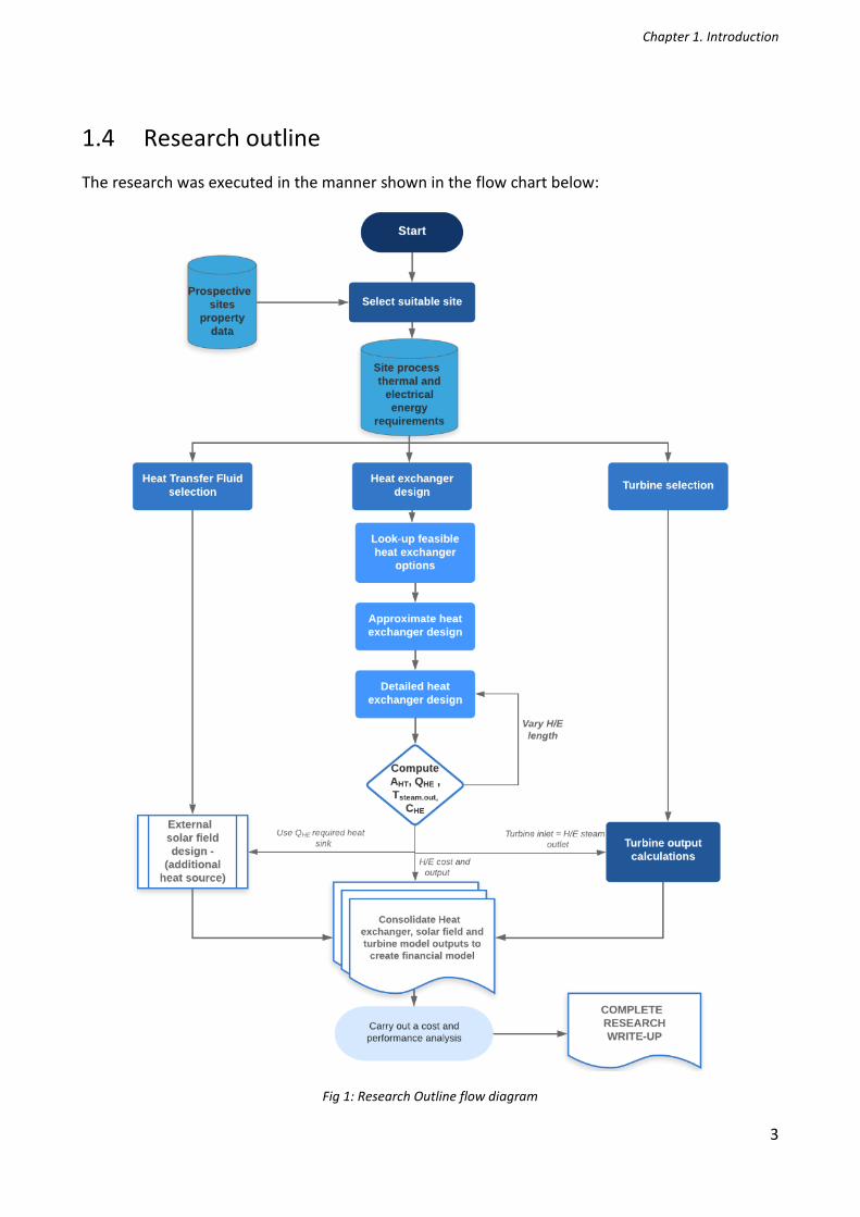
1.4 Research outline
The research was executed in the manner shown in the flow chart below:
Fig 1: Research Outline flow diagram
Chapter 1. Introduction
4
1.5 Expected outcomes
At the end of this research, the following will be produced:
• A framework for the integration of process steam boilers with steam turbine generator sets
for power generation whilst meeting process thermal load requirements.
• A heat exchanger design to raise the steam conditions from dry saturated to superheated.
• An indication of financial feasibility and typical costs associated with the uptake of such a
project.
1.6 Disclaimer
Techno-economic studies can be highly site, industry and country specific. This project does not
claim to be a comprehensive feasibility of the chosen site. Rather, it is meant to identify and
highlight certain aspects that could make solar augmentation of an existing process steam plant
potentially viable, or completely non-viable.

Chapter 2. Literature Review
5
2. Literature Review
Literature pertinent to this study will be reviewed in this chapter. The chapter begins by looking at
the existing process steam plants and their operating thermodynamic cycle, the Rankine cycle.
Following that, the concept of cogeneration will be presented, focusing on what has been put
forward to date, its relevance to this study and how a process steam plant can be converted into a
combined heat and power plant. Solar thermal systems, heat exchangers, steam plants and steam
plant economics will be explored subsequently as they are important in this study.
2.1 Process steam plant and the Rankine cycle
A steam plant is a system that utilizes a high-pressure boiler to generate steam for heating and or
power generation. Traditional process steam plants produce steam at mostly dry saturated
conditions and use it as a heat source for thermal processes. The Rankine cycle on the other hand
is a heat engine cycle, which uses water as the working fluid to convert heat energy to mechanical
work whilst the working fluid goes through phase changes [2]. The mechanical work is
predominantly further converted to electrical energy. Described first in 1859 by William Rankine,
thermal power plants worldwide utilize the cycle for power generation. It has four physically
different processes, which use different equipment joined by pipework to make a closed cycle
(Figure 2).
Figure 2: Rankine cycle basic flow diagram
The simple ideal cycle, with superheat consists of the following stages [3];

Chapter 2. Literature Review
6
• 3 - 4: Isentropic compression in the boiler feed pump,
• 4 - 1: Constant pressure heat addition in the boiler,
o 4 – 5: Subcooled liquid heat addition to boiling point,
o 5 – 6: Latent heat addition to change state from liquid to gas,
o 6 – 1: Superheating to increase thermal state at turbine inlet,
• 1 - 2: Isentropic expansion in the turbine,
• 2 - 3: Constant pressure two-phase heat rejection in the condenser.
Figure 3: Ideal Rankine cycle T-s diagram
Several enhancements to the simple cycle have been made to improve the cycle efficiency by either
increasing the thermal state of the high-pressure steam at the turbine inlet or reducing the thermal
state of the low-pressure steam at the condenser outlet. This can be realized in one of these ways:
• Increasing boiler pressure,
• Increasing boiler exit temperature,
• Decreasing condenser pressure,
• Feedwater heating – (Increasing the enthalpy of the working fluid at boiler inlet),
• Reheating – (increasing the enthalpy of the high-pressure turbine stage exhaust, before
feeding it into the intermediate/ low pressure turbine stage).
In this study, the objective is to increase the thermal state after boiler heat addition to superheated
steam, which allows the steam to be first expanded in a turbine for power generation, and then use
the turbine exhaust for process heating applications. Given that the original steam plant layout is
only for saturated process steam, the introduction of superheating will enable the simultaneous
production of heat and power, which is widely known as Cogeneration.

Chapter 2. Literature Review
7
2.2 Cogeneration
Cogeneration is the production of two usable sources of energy, usually heat and electricity, from
the same fuel [4] leading to considerable fuel cost savings. Practical use of the technology dates to
the earliest commercial Edison coal- fired power plants in the late 1800s [5]. The OPEC crisis of 1973
led to the use of renewables to augment supply, giving birth to the world’s first independent power
producers tied to the national grid and formulation of the Public Utility Regulated Policy Act widely
known as PURPA. This law paved the way for large scale cogeneration and independent power
production [5].
According to the International Energy Agency [4], cogeneration coupled with renewables leads to a
supply of low carbon electricity and heat which is vital to the realization of a sustainable future. It is
also a vector of energy efficiency, as the production of the heat and power occurs at the place of
consumption, minimizing transmission line losses. Classification of cogeneration systems is based
on the sequence of energy use, being either topping or bottoming cycles. Topping cycles (the most
common ones) produce electricity first and use the waste heat for industrial or district heating.
Bottoming cycles on the other hand produce useful heat first for high-temperature thermal
processes (glass and steel industries) then use the waste heat for power generation in heat recovery
steam generators.
Today, many process steam plants employ cogeneration, mainly steam turbine topping cycles to
provide electricity to meet plant demand and the turbine exhaust for process thermal load. The
researcher visited a few process steam plants in Zimbabwe to get an in-depth knowledge on how
the cogeneration systems are set up, and the findings are given in detail in the next chapter.
However, a point to note in this literature survey is that the process steam plants with cogeneration
were designed with cogeneration in mind from the onset, hence use utility water tube boilers for
steam generation. The process steam plants under investigation in this study use fire tube boilers,
which produce only dry saturated steam which is not adequate for power generation. A steam
turbine topping cycle (STTC) will be employed, generating the electricity from the superheater
outlet, and then using the turbine exhaust as the process steam. A steam turbine topping cycle
(with a back-pressure turbine) is shown in the figure below:

Chapter 2. Literature Review
8
Figure 4: Cogeneration – Back Pressure Steam turbine topping cycle
The turbine options in a STTC are either a back pressure (shown above) or extraction-condensing
type. In the back-pressure turbine STTC, the steam is exhausted from the turbine at a pressure above
atmospheric which is equal to the process steam pressure requirement. Also note that there is no
condenser in the back-pressure steam turbine topping cycle because the process plant “acts as the
condenser”. The advantages of the backpressure STTC are the simple configuration, lower capital
costs as no condenser is required (low or no need of cooling water as the turbine exhausts to the
process plant which acts as the condenser) and a higher thermal efficiency as all the heat added in
the boiler is fully utilized in both the turbine and process plant. The downside of a backpressure
STTC is that there is little or no flexibility in matching the electrical power output to the demand as
the thermal load controls the turbine output.
The second option, the extraction-condensing STTC uses an extraction-condensing/pass-out turbine
which partly bleeds steam to the process and partly condenses the remaining steam (detailed
explanation on the differences between the two turbine types is outlined in Section 2.5 below). The
advantage of the extraction-condensing turbine is that the electrical power output control is
independent of the thermal load requirement, thus the cogeneration plant can match the electrical
demand to the turbine output. The disadvantage however of this set-up is that the thermal
efficiency is lower as heat is lost to the surroundings in the condenser and higher capital costs as
there is need for a condenser and cooling water supply.

Chapter 2. Literature Review
9
2.3 Solar thermal systems
The conversion of solar energy to mechanical and electrical energy is as old as 1872 when a steam
powered press was exhibited at the Paris Exposition [6]. The system used concentrating collectors
to supply heat to the heat engines and from that other solar thermal-mechanical systems were
developed for small-scale applications, mostly solar water pumping.
Basic energy conversion in solar thermal systems is shown in the picture below:
Figure 5: Solar thermal system basic layout
The energy conversion process consists of:
• Solar energy collection by either a flat plate or concentrating collector (parabolic trough
shown above),
• Storage, in indirect integration solar systems, which usually use molten salts as thermal
storage heat transfer fluid,
• Heat addition in the heat exchanger,
• Conversion of heat energy to useful work in the heat engine.
Flat plate thermal collectors are usually utilized in small-scale solar thermal systems like home water
heating systems. Large scale solar thermal systems like solar power plants, use various kinds of focus
systems for concentrating the heat with a higher efficiency despite being more expensive and
complex to construct. The four main concentrated solar collector types are: parabolic trough
systems, linear Fresnel systems, power towers also known as central receiver systems and parabolic
dishes. Present day commercial Concentrated Solar Power (CSP) projects employ parabolic troughs
as they are the most developed CSP technologies with measured optical efficiencies as high as 78%
in the SkyFuel trough systems [7]. Power towers, though being more efficient and offering better
energy storage options are less developed than the trough system.

Chapter 2. Literature Review
10
Solar thermal technologies in power plants can be utilized in one of two ways: stand-alone solar
thermal power plants (STPPs) or solar assisted power generation (SAPG). SAPG is a synergy of solar
and fossil fuels which combines the environmental benefits of the solar energy and scale, reliability
and efficiency of traditional fossil fuel plants [8] . According to Pierce [8], a SAPG plant is 25% more
efficient and 1.8 times more cost effective than a STPP of equal size of parabolic trough solar
technology. Other authors, Petrov et al [9]; Yang et al [10] and Hu et al [11] have also shown that
SAPG utilizes solar thermal energy better than stand-alone STPPs.
SAPG systems are employed in countries with a rich fossil fuel resource base and high solar
insolation, which makes it relevant for Zimbabwe as it has an abundance of both the coal resource
and solar resource (annual average of 2100 peak sunshine hours per annum [12]). In utility high
scale systems, solar thermal energy is integrated for: production of main steam (superheating), or
production of intermediate steam (reheating) or preheating of feedwater. There are two options of
augmentation: direct and indirect integration. In direct integration, the steam is directly heated in
the solar field whereas in indirect heating, an additional heat exchanger with a separate solar loop
is employed. According to Petrov et al [13], the feedwater heating is the most effective in large
utility scale projects [13].
The world’s first true solar-coal hybrid project was located at Cameo Generating station in Colorado,
USA [14] (shown in the figure below):

Chapter 2. Literature Review
11
Figure 6: Cameo Generating Station SAPG system [15]
The system used parabolic troughs to heat mineral oil heat transfer fluid to ~300℃, which was used
to preheat feedwater for one of the 49-MW plant’s coal fired units. Commissioned in 2010, the plant
underwent a 7-month demonstration programme and showed positive results with an increase in
overall plant efficiency 1% and reduction in coal demand and emissions. It was decommissioned
after the 7-month pilot project. Another notable feedwater heating project was the New South
Wales Novatec Solar, Liddell power station solar boost. The 9.3MWth plant commissioned in 2012,
cut annual 2CO emissions by ~ 5000 tonnes but was closed down in 2016 due to technical and
contractual issues [16].
Kogan Creek A Power station solar boost project was a SAPG project which produced main steam to
add 44MW to the 750MW Kogan Creek Power Station during peak solar conditions in Queensland,
Australia [17]. The system, the largest in the capacity for SAPG to be ever developed commercially,
used compact linear Fresnel reflector technology. Construction began in 2012 but the project was
never completed due to technical and contractual issues. In 2016, the project was discontinued as
it could not be deployed commercially without a further substantial capital investment. Findings
from the project showed that location selection for a solar thermal addition plays a pivotal role given
that solar projects favour high insolation areas (arid and semi-arid areas). These high insolation
areas usually do not coincide with existing standalone utility coal fired plants which are in areas with

Chapter 2. Literature Review
12
an abundant supply of cooling water. Another key issue was the use of technology, which was in
early stages of development.
The figure below shows a typical solar parabolic trough system, with thermal storage and a power
cycle:
Figure 7: Concentrated Solar Power Parabolic Trough system adapted from the US Department of Energy [18]
The physical trough model is one of the US National Renewable Energy Laboratory (NREL) open-
source System Advisor Model (SAM) software’s models, which is designed for power generation
applications. SAM is a performance and financial model used to help renewable energy industry
researchers, technology developers, project managers and engineers make informed decisions
when sizing and designing solar projects [18].
Another model in the SAM NREL software package, which is similar to the CSP physical trough is the
industrial process heat parabolic trough (IPH), which instead of the power block assumes that the
heat from the solar field is used for thermal applications rather than driving a power cycle. In this
study, the IPH model will be used in the solar field design because the heat from the field is used to
heat up dry saturated steam to superheated steam. No thermal storage will be employed as it is
beyond the scope of this study and will escalate the capital costs, despite being the most effective
way of harnessing the solar resource. Given that indirect integration will be employed, a suitable
heat exchanger will be designed to superheat the steam.

Chapter 2. Literature Review
13
2.4 Heat exchanger design
Heat exchangers are process industry work horses, widely employed in thermal applications where
there is need for heat transfer between two or more process fluids. The heat transfer process
(heating or cooling) and the process fluids determine the type of heat exchanger to be used. Most
applications have several alternative designs and final selection must be done based on different
performance and cost factors [19] for example:
• For small duties, annular heat exchangers are the most feasible option as they are cheaper
to manufacture.
• For heavier duties where sealing gaskets do not give rise to operational difficulties, plate and
frame heat exchangers are the heat exchanger of choice. However, where pressure and
temperature of process fluids exceed 40bar and 350˚C [20], sealing becomes a problem and
the plate and frame heat exchanger becomes uneconomical to use.
• For heavier duties with high process pressures and temperatures, the shell and tube heat
exchangers become the cheaper option.
• Where space is limited, compact exchangers like the plate-fin, tube fin and rotary
regenerators are employed. However, plate-fin and tube fin exchangers can only be
considered if the working fluid does not pose significant fouling characteristics. Fouling
significantly increases the heat exchanger maintenance costs and diminishes the heat
exchanger long term performance.
• Where hygienic demands are high and it is desired to ensure no cross contamination
between the hot and cold fluid, plate heat exchangers are used.
Given the above considerations, and the process and heat transfer fluids’ operating temperature
and pressure, the shell and tube heat exchanger (STHE) is the most feasible option and the
subsequent sub-sections will focus on the thermal design of shell and tube heat exchangers.
2.4.1 STHE Basics
The basic layout for a shell and tube heat exchanger, with one tube pass and multiple shell passes
is shown below:

Chapter 2. Literature Review
14
Figure 8: Shell and Tube Heat Exchanger layout
Various tubes are arranged into a bundle, kept in place by a tube sheet on each end of the entire
tube length. The tube bundle is then welded into the shell, which is usually a steel pipe of required
shell material. However, only shell diameters up to 24” are fabricated from steel pipes [21]. Above
that, steel plates are rolled into the desired shell diameter. Baffles are used to both direct the shell
fluid into multiple passes and support the tubes (maximum unsupported span of the tubes is
specified in Tables R-4.41 and CB-4.41 of the TEMA standards [21]). The ends of the shell are
designed based on the fluid operating pressures and the whole component can be simplified into a
schematic diagram showing the flow of the hot and cold fluid streams as shown below:
Figure 9: Heat Exchanger Schematic
where the subscripts 𝑖, ℎ; 𝑖, 𝑐; 𝑒, ℎ 𝑎𝑛𝑑 𝑒, 𝑐 denote the hot fluid inlet, cold fluid inlet, hot fluid exit
and cold fluid exit respectively. The fundamental heat transfer equation states that:
LMTDQ UA T= (2.1)
Where Q is the heat transfer rate, U is the overall heat transfer coefficient, A is the heat transfer
area and LMTDT is the logarithmic mean temperature difference, calculated as shown in (2.2)
below for a pure counter flow arrangement:

Chapter 2. Literature Review
15
, . , ,
, .
, ,
( ) ( )
ln
i h e c i c e h
LMTD
i h e c
i c e h
T T T TT
T T
T T
− − − =
− −
(2.2)
The logarithmic mean temperature difference (LMTD) can also be expressed as follows:
1 2
1
2
ln
LMTD
T TT
T
T
− =
(2.3)
Where 1T and 2T are the temperature differences between flows on the left-hand side and
right hand side of the graphs shown in Figure 10 below:
Figure 10:Temperature differences for different heat exchanger flow arrangements
where the flow deviates from pure counter flow or parallel flow, a flow correction factor, TF , is
multiplied to LMTDT to give the true temperature difference as follows:
true T LMTDT F T = (2.4)
The flow correction factor is a function of the fluid temperatures and the number of shell and tube
passes [22] and is determined graphically, from graphs developed by Kern and other researchers
using a correlation of two dimensionless constants, R and S defined below:
, ,
, ,
i h e h
e c i c
T TR
T T
−=
−
, ,
, ,
e c i c
i h i c
T TS
T T
−=
−
The overall heat transfer coefficient is a measure of how well heat is transferred between the
different heat transfer media. In this instance, heat is transferred by convection from the fluids to
the wall surface, and conduction through the tube wall separating the hot and cold fluids. The
overall heat transfer equation, assuming clean conditions is calculated as follows [19, p. 264]:
ln
1 1
2
oo
i o
i o i
DD
D DU
h k h D
= + +
(2.5)
Chapter 2. Literature Review
16
Where, , , ,o i oh h k D and iD are the shell-side fluid convective heat transfer coefficient, tube-side
fluid convective heat transfer coefficient, tube wall thermal conductivity, tube outer and inner
diameter respectively. The convective heat transfer coefficient is defined as the rate at which heat
is transferred between a fluid and a solid surface per unit surface area of heat transfer per unit
temperature difference. It is a function of the fluid properties, Nusselt number and thermal
conductivity and the heat transfer surface dimensions (the diameter if it is a cylindrical section).
The first law of thermodynamics must be satisfied in any heat exchanger design, both at macro
and micro level [23] thus by principle of conservation of energy;
0h cQ Q+ = (2.6)
i.e., the heat gained by the cold stream equals the heat lost by the hot stream where,
( ) , ,h h e h i hQ m h h= − (2.7)
And
( ) , ,c c e c i cQ m h h= − (2.8)
Which reduces to
( ) ( ).
, , , ,true h ph e h i h c pc e c i cQ UA T m c T T m c T T= = − = − − (2.9)
if the heat transfer process occurs at constant pressure and pc is the specific heat capacity at
constant pressure.
Another heat exchanger heat transfer analysis method which is widely used is the effectiveness
method, popularly known as the -NTU method, where and NTU denote the effectiveness and the
Number of Transfer Units of the heat exchanger respectively. This method was formally introduced
in 1942 by London and Seban [23] and relates the heat transfer rate to the fluid flow rates,
effectiveness and temperature as follows:
. .
maxQ Q= (2.10)
.
maxQ is the theoretical maximum possible heat transfer rate which would be obtained if the heat
exchanger had a pure counterflow arrangement, infinite surface area and no heat losses to the
surroundings. It is calculated as follows:
.
min , ,max ( )i h i cQ C T T= − (2.11)
and,

Chapter 2. Literature Review
17
. .
min , ,min( ; )h cp h p cC m c m c= (2.12)
The effectiveness, , is a measure of how the heat exchanger performs and relates the actual heat
transferred by the heat exchanger to its maximum possible theoretical value. It is a dimensionless
factor, with a range of values between zero and 1
( ; )rf NTU C =
Where rC is the heat capacity ratio:
.
minmin
.
maxmax
( )
( )
p
r
p
m cCC
C m c
= =
(2.13)
The number of transfer units (NTU) designate the non-dimensional “heat transfer size/ thermal size”
of the heat exchanger [23], calculated as the ratio of the overall conductance and minimum heat
capacity rate as follows:
min min
1
A
UANTU UdA
C C= = (2.14)
Various analytical equations exist relating NTU and , and is a function of the specific flow
arrangement and fluid conditions. In the case where there is one shell pass, the -NTU correlation
is as shown in equation (2.15) below [24]:
( )( ) ( )
( ) ( )
21
21
11
2
11
12 1 1
1
r
r
NTU C
r rNTU C
eC C
e
−− +
− +
+
= + + + −
(2.15)
where the subscript 1 denotes values for the single pass shell. For multiple shell passes and multiple
tube passes (n shell passes and 2n, 4n… tube passes), the effectiveness-NTU correlation is a function
of the single shell, multi-tube pass effectiveness and is calculated as follows [24]:
1
1 1
1 1
1 11
1 1
n n
r rr
C CC
−
− − = − −
− −
(2.16)
where all symbols have their usual meanings. Given that the baffles direct the shell fluid, the chosen
baffle type plays a pivotal role in the direction of shell fluid flow (parallel for longitudinal baffles,
cross-flow for transverse baffles or mixed flow). The flow direction also has a bearing on the shell-
side heat transfer coefficient with flow parallel to the heat exchanger achieving pure counterflow
and having the highest possible heat transfer. In shells where transverse baffles are employed, flow
ceases to be pure counter-flow, but a mixture of cross and parallel flow. Although transverse baffles
Chapter 2. Literature Review
18
increase turbulence of the shell fluid [23], increasing the shell-side velocity, their heat transfer rate
is less than that of a pure counterflow heat exchanger of the same length due to losses in the baffle
clearances and window zones. However, according to Cayglan and Buthod [25], where the number
of transverse baffles are greater than ten, the heat exchanger is assumed to be a pure-counterflow
heat exchanger. Where the flow is pure counter-flow and the heat capacity ratio is less than 1, the
NTU equation is given as:
(1 )
(1 )
1
1
r
r
NTU C
NTU C
r
e
C e
− −
− −
−=
− (2.17)
And where the hot and cold fluid heat capacities are the same, i.e. 𝐶𝑟 = 1,
1
NTU
NTU =
+ (2.18)
2.4.2 Design Considerations
The objective in heat exchanger design is to ensure that it performs its thermal duty at the lowest
cost whilst still maintaining in-service reliability [26]. There is always a trade-off between heat
exchanger size, cost and pressure drop.
The general inputs in shell and tube heat exchanger thermal design are hot and cold fluid properties
(pressure, temperature) and flow rates. Design of a new heat exchanger means selection of a heat
exchanger construction type, flow arrangement, tube and shell material and physical size to meet
the specified heat transfer and pressure drop requirements [23]. The common heat exchanger
design problems are rating and sizing problems. In a rating problem, the performance evaluation
(determination of heat transfer rate, outlet fluid temperatures and pressure drop) of an existing or
already sized heat exchanger is done. The sizing problem determines the physical size (length, width,
height, and surface area) of a heat exchanger for a given duty [23].
Whether it is a rating or sizing problem, all designs of STHEs have two aspects, namely thermal and
mechanical design. Thermal design focuses on the determination of the heat transfer area, tube and
shell layout and fluid pressure drops. The designer then must check if the mechanical parts can
withstand the operational conditions without failure of components in the mechanical design.
Optimum design of STHEs involves the consideration of the following design parameters [22]:
Process considerations
i. Fluid flow arrangements and properties.
ii. Shell and tube side pressure drop limits.
iii. Shell and tube side velocity limits.

Chapter 2. Literature Review
19
Mechanical considerations
i. Heat exchanger Tubular Exchanger Manufacturers Association (TEMA) layout.
ii. Tube specifications such as size, layout, pitch, and material.
iii. Setting design limits on tube length.
iv. Shell specifications - material, baffle cut, baffle spacing and clearances.
v. Setting design limits on shell diameter.
vi. Thermal cycles for fatigue prediction.
vii. Thermal gradients during transients which influence the design of thick-walled
components like the tube sheet and shell attachments.
Heat exchangers with shell inside diameters up to 100” and max design pressure of 3000psi [21] are
manufactured to the standards set out by the Tubular Exchangers Manufacturers Association
(TEMA). The above limits are enforced to limit the shell wall thickness to 76mm for ease of
manufacturing, and the 9th Edition of the standard will be referenced throughout this design.

Chapter 2. Literature Review
20
2.4.3 TEMA Heat Exchanger types
Figure 11:TEMA Exchanger types adapted from Standards of the Tubular Exchanger Manufacturers Association, 9th Edition [21]
TEMA type designation, shown in Figure 11 above, is by letters describing the front end, shell type,
rear end in that order, followed by the size which has the nominal shell diameter (inside shell

Chapter 2. Literature Review
21
diameter rounded in inches) and nominal length of tubes in inches, followed by the metric size in
brackets. A typical example for a TEMA heat exchanger designation is:
SIZE 19-84 (483-2134) TYPE BGU
meaning a U-tube exchanger with bonnet type stationary head, a split flow shell, 19” (483mm)
shell inside diameter and straight tube length of 84” (2134mm).
The right shell choice leads to an optimized heat transfer rate [27]. TEMA standardized 7 types of
shells, described in detail below.
The type E, single pass shell is the most common for single phase shell fluid applications due to its
simplicity, ease of manufacture and subsequent low cost. Tubes can be single or multiple pass and
are supported by transverse baffles which also act as shell fluid multi-pass compartments. The most
effective heat exchanger is the type E shell with a single tube pass arrangement as it approaches a
pure counterflow arrangement.
Where a process requires a larger heat transfer area, such that more than one tube pass is used, or
if there is a temperature cross in the type E shell, the F shell is used to achieve a counter-current
flow and achieve effectiveness values as close to the 1-1 pass arrangement. It has a longitudinal
baffle separating the type E shell into two distinct sections. However, the disadvantage of the F shell
is baffle leakage and conduction heat losses to the baffle which reduces the shell side heat transfer
coefficient.
TEMA G (spilt flow) and H (double split flow) shells are employed where the pressure drop is
supposed to be kept at the minimum. The G shell has no baffles, just a single support in the middle
and fluid enters in the middle section and divides into two, hence the term split flow. Where the
tube lengths are longer, the H shell is employed which is like two G shells combined into one.
The J-shell is used where the pressure drop in the shell is too large for the E shell to handle [27]
which can lead to tube vibration. The shell side velocity in this shell is half that of the type E shell,
which implies that the pressure drop will be almost a quarter of that of the E shell. Fluid enters at
the centre, splits into two streams and leaves through two separate outlets which can be
recombined outside the shell.
The X shell is used for pure cross flow design where it is desired to have little or no pressure drop in
the shell. Fluid enters from one side and leaves at the direct opposite end of the inlet nozzle. The
final shell type is the K shell used for partially vaporizing the shell fluid in kettle reboilers. Almost
like the X shell, the K type has an enlarged shell to allow for vapor disengagement and minimize
carryover.

Chapter 2. Literature Review
22
2.4.4 Fluid Flow Allocations
Fluid flow allocation to either the shell side or tube side has a huge impact on the heat exchanger
effectiveness, maintenance requirements, initial cost and cost of replacement parts [28]. Practical
guidelines state that the flow arrangements for optimum operation should be as follows:
• Higher pressure (HP) fluid in the tubes as they have smaller diameters and nominal wall
thickness, making the design cheaper than having the fluid in the shell which will then call
for a thicker shell to withstand the pressure. However, if the HP fluid can only be put in the
shell, it is necessary to make the shell smaller in diameter and long length to minimize costs.
• Higher fouling fluid in the tubes as they are easier to clean using mechanical methods
compared to the shell.
• Lower heat transfer coefficient fluid in the shell.
• If all properties are almost similar, the corrosive fluid in the tubes as it is less expensive to
use special alloys for corrosion resistance in the tubes than the shell alloys.
• Lower velocity fluid in the tubes as the lower the fluid flow velocity, the higher the fouling
rates. Acceptable tube side velocity varies with the fluid, with most liquids ranging from 0.9-
1.52m/s and gases ranging from 15-30m/s.
2.4.5 Heat transfer model selection
Heat transfer model selection depends on the heat transfer process (sensible, boiling or
condensing); surface geometry of both the tube and shell side; fluid flow regime (laminar, turbulent
or mixed) and surface orientation (horizontal or vertical) [22]. In this study, the heat transfer process
is for sensible heat transfer and only the sensible heat transfer models in turbulent flow will be
discussed for both the shell and the tube -side.
Shell-side film coefficient methods
Stream analysis
In this method, usually employed in computer thermohydraulic programs for heat exchanger design,
the pressure drop across the baffles is balanced for each possible flow path, including leakage flow
areas [22].
Kern Method [29, p. 137]
The original Kern method was an adaption of the Nusselt equations to suit evaluation of fluid
conditions at film temperature for streamline flows with Reynolds numbers in the range of 1800 –
2100. The Colburn method on the other hand, is applicable to turbulent flow in industrial heat
exchangers using standard tube pitch designs. Using existing experimental techniques and different

Chapter 2. Literature Review
23
heat transfer fluids, Kern was able to show that for sensible heat transfer with turbulent flow in
segmented baffle shells:
0.14
10.55 30.36 Re Pr t
s s s
wall
Nu
= (2.19)
where the subscripts 𝑠 and 𝑡 denote the shell and tube side fluids respectively and the Reynolds
and Prandtl numbers are calculated as follows:
Re s es
s
G D
= and
.
.
Prp s s
s
s
c
k
=
where 𝐺𝑠 is the shell-side mass velocity and 𝐷𝑒 is the equivalent shell diameter, calculated as shown
in (2.29). This Nusselt correlation by Kern strongly agrees with the Colburn and Short methods [29].
Bell-Delaware Method [19, pp. 275-277]
The Bell-Delaware method is an improvement of the Kern method and corrects for heat transfer
coefficient reduction due to leakage flows by accounting for the losses due to leakages through the
tube holes and baffle clearances, by-pass flows and effect of baffle configuration on the shell-side
fluid flow pattern. In this method, the ideal shell side heat transfer coefficient is first calculated using
the Kern method, then correction factors for the leakage flows are calculated and factored in the
ideal heat transfer coefficient to give the corrected actual heat transfer coefficient.
Tube-side film coefficient methods
Dittus-Boelter Equation [19, p. 105]
This is the most popular correlation used to calculate the average Nusselt number for fully
developed (both thermally and hydrodynamically) turbulent flows in liquids and gases with a range
of Reynolds numbers, Re>10000; Prandtl number 0.7<Pr<150 and length to diameter ratio of tubes
greater than 10. It states that:
0.80.023 Re Prn
D DNu = (2.20)
where the coefficient n is either 0.3 when the tube-side fluid is being cooled or 0.4 when the tube-
side fluid is being heated. However, the Dittus-Boelter equation is less accurate for rough tubes and
flows characterized by large temperature variations.

Chapter 2. Literature Review
24
Sieder-Tate Equation [29, p. 103]
The Sieder-Tate equation was developed to account for the effect of variation of fluid viscosity with
temperature, particularly in instances where the difference between the fluid and surface
temperatures is very large. It states that:
0.14
0.8 0.330.027 Re Prfluid
D D
wall
Nu
= (2.21)
for flows in horizontal and vertical pipes involving inorganic liquids, aqueous solutions and gases
with a range of Reynolds numbers, Re>10000; Prandtl number 0.7<Pr<700 and length to diameter
ratio of tubes greater than 60.
Gnielinski Equation [24, p. 515]
Although equations (2.20) and (2.21) are easily applied and satisfactory for many heat transfer
applications, they result in errors as large as 25% [24] and a more recent correlation, the Gnielinski
correlation can be used. It is valid for a wide range of Reynolds numbers, including the transition
region and reduces the error to less than 10%. It states that:
( )( )
( ) ( )12 2
3
Re 1000 Pr8
1 12.7 Pr 18
D
D
f
Nuf
−
=
+ −
(2.22)
Where f is the Darcy friction factor, which accounts for the frictional losses in the pipe or duct,
obtained from the Moody diagram.
The VDI-Mean Nusselt method [19, pp. 73-79]
In this method, the average heat transfer coefficient of the whole tube bank is evaluated, as
opposed to a single tube in cross-flow [22] and bases the Reynolds number calculation on the
maximum flow velocity, rather than upstream velocity. It states that:
0.34
1 2Re Prm
mNu a F F= (2.23)
Where a and m are correlation constants and 1F and 2F are correction factors for surface to bulk
physical property variations [22].
A number of computer thermohydraulic design programs have been developed to aid in the design
and optimization of heat exchangers like CC-Therm and CHEMCAD [30], and automatically select

Chapter 2. Literature Review
25
the applicable heat transfer model for a given set of boundary conditions. In this study, an iterative
optimum sizing will be done using a MathCAD analytical calculation, developed for this purpose.
2.4.6 Tube design
Tube diameter and material
Standard tube sizes are available from 1 4⁄ " to 2” outer diameter, OD, with the common sizes being
ODs of 3 4⁄ " and 1”. The tube wall thickness is defined by the Birmingham wire gauge and standard
tube sizes are specified in Table RCB-2.21 of the TEMA standard. Tube materials are copper, steel
and alloy steel like aluminium-bronze, copper-nickel and admiralty, with other application specific
materials, diameters and gages still being acceptable.
Tube length and count
Straight and U-tube exchangers have common standard lengths of 12, 15, 18, 20 and 30ft. Other
sizes can also be used. Tube length determines the heat transfer area, but very long unsupported
lengths pose threats of in-service vibration and shell side distribution problems [22].
Tube count refers to the number of tubes in the tube bundle and dictates the velocity of fluid inside
the tubes. Acceptable tube side velocity varies with the fluid, with most liquids ranging from 0.9-
1.52m/s and gases ranging from 15-30m/s [19]. These values are however very dependent on the
type of fluid and fluid properties like viscosity, with Therminol VP-1, a thermal oil having acceptable
velocity ranges of 0.36 – 4.97m/s according to its manufacturer [31]. The minimum tube side
velocity is set to avoid settling of the fluid particle which increases fouling and the maximum to
avoid too much turbulence which leads to tube erosion. The desired flow velocity determines the
tube count. The bundle layout is determined by geometric factors, dimensions and clearances,
removal of scavenger air, etc., with the tube layout and tube pitch being the critical deciding factors
[32]. Table 11-3 of Perry’s Chemical Engineers’ Handbook sets out standard tube count data.
The tube count is calculated by dividing the shell circle area by the projected area of the tube layout
[33]. Figure 12 below shows typical baffle and bundle geometries useful in calculating the tube
count:

Chapter 2. Literature Review
26
Figure 12: Baffle and tube bundle geometries [32]
According to Taborek, a simple estimation formula can be used for fixed tube sheets with a single
tube pass and no tubes removed at the entrance and exit areas as follows [32, pp. 3-8]:
2
2
0.7854 ctlt
tp
DN
CL L
=
(2.24)
where, ctlD is the centreline tube limit diameter, calculated as the difference between the outer
limit tube diameter and the tube outside diameter; CL is the tube layout constant and tpL is the
tube pitch. On the other hand, defining the tube count from first principles reduces the expression
to [33, p. 76]:
2
2 24
St
o
CTP DN
CL PR D
=
(2.25)
Where CTP is a constant for tube passes defined as 0.93, 0.9 and 0.85 for one, two and three tube
passes respectively, SD is the shell inside diameter and PR is the ratio of the tube pitch to the tube
outside diameter. Knowing that the tubes have a limit of how far they go as far as the shell inside
diameter is concerned (which is accounted for in Taborek’s equation by using the centreline limit
diameter) and also to account for different tube pass arrangements in the analytical modelling of
the heat exchanger, the researcher combined aspects of equations (2.24) and (2.25) to calculate
the tube count as follows:

Chapter 2. Literature Review
27
2
24
ctlt
tp
CTP DN
CL L
=
(2.26)
Tube clearance, pitch and layout
Too small a distance between two adjacent tube holes weakens the tube sheet and thus a
considerable amount of space should be left between tube holes to maintain tube sheet structural
integrity [29]. Tube clearance is the shortest distance between two adjacent tube holes and tube
pitch is the shortest centre to centre distance between adjacent tubes [29]. The tube pitch is
calculated as follows:
tp oL D C= + (2.27)
Where tpL is the tube pitch in the transverse direction, oD is the tube outer diameter and C is the
tube clearance. The pitch is also dependant on the tube layout with the common layouts being
outlined below:
Figure 13:Tube layouts adapted from NPTEL Chemical Engineering Design Module I [33]
The square pitch is most widely used because the tubes are accessible for external cleaning and it
also has a lower pressure drop if the shell fluid flows in the direction shown above. Triangular
pattern provides a more robust tube sheet construction [22] but should not be used where
mechanical cleaning methods are used to clean the shell. According to TEMA, the minimum tube
pitch should be 1.25 times oD .
Tube sheet
Tubes are fixed to the tube sheet, which also acts as the barrier between shell-side and tube -side
fluids. Because the tube sheet is exposed to the most adverse of the operating conditions (varying
temperatures and pressures from shell and tube-sides), care must be taken in its design to avoid
either shear or bending failures in-service. TEMA specifies the minimum tube sheet thickness as

Chapter 2. Literature Review
28
greater than 75% of oD . Detailed design of the tube sheet is specified in Appendix A of the TEMA
Standard.
2.4.7 Shell design
The objective in shell design is to specify a shell which fits the tube bundle, at the same time
performing its thermal duty in the allowable range of fluid pressure drop. The method which will be
discussed in this section is the Taborek modification of the Bell-Delaware method as it gives a more
accurate result.
Shell diameter
The shell diameters are not standardized according to TEMA, but the selection of a shell inside
diameter should be such that the tube count is within limits for that size. Pipe and plate shells are
governed in accordance to ASTM/ASME pipe specifications [21]. The minimum shell thickness is
selected such that the whole shell withstands the pressure differential exerted on it, as well as
accounting for a corrosion allowance set in the TEMA standard.
The flow area in the shell is a function of the shell diameter. However, because of the presence of
the tube bundle in the shell, the shell flow area becomes non uniform necessitating the need of
finding a shell-side equivalent diameter, an approximate diameter which accounts for the non-
uniform fluid flow in the shell. It is a function of the hydraulic radius, which is the ratio of the cross-
sectional area of a non-circular flow conduit to its wetted perimeter. According to Kern [29], the
direction of flow in the shell is partly along and partly across the length of the tubes, the flow area
is variable from tube row to row. Because the hydraulic radius based upon the flow area across any
one row could not distinguish between square and triangular pitch [29], this led to the formulation
of the equivalent shell diameter which combines both the size and pitch of the tubes and their type
of pitch by considering the flow along (instead of across) the tube length to be four times the
hydraulic radius. The shell equivalent diameter is calculated as [29]:
4
e
FreeAreaD
Wettedperimeter
= 1 (2.28)
Which reduces to:
2 244
tp o
e
o
L D
DD
−
=
(2.29)
1 Kern uses free area to avoid confusion with free-flow area, an actual entity in the hydarulic radius [29]
Chapter 2. Literature Review
29
For a design with square pitch tube arrangement.
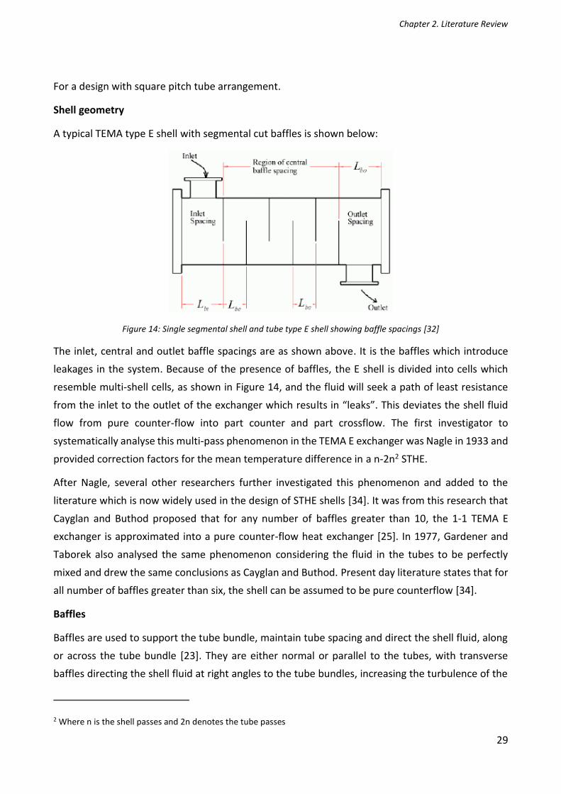
Shell geometry
A typical TEMA type E shell with segmental cut baffles is shown below:
Figure 14: Single segmental shell and tube type E shell showing baffle spacings [32]
The inlet, central and outlet baffle spacings are as shown above. It is the baffles which introduce
leakages in the system. Because of the presence of baffles, the E shell is divided into cells which
resemble multi-shell cells, as shown in Figure 14, and the fluid will seek a path of least resistance
from the inlet to the outlet of the exchanger which results in “leaks”. This deviates the shell fluid
flow from pure counter-flow into part counter and part crossflow. The first investigator to
systematically analyse this multi-pass phenomenon in the TEMA E exchanger was Nagle in 1933 and
provided correction factors for the mean temperature difference in a n-2n2 STHE.
After Nagle, several other researchers further investigated this phenomenon and added to the
literature which is now widely used in the design of STHE shells [34]. It was from this research that
Cayglan and Buthod proposed that for any number of baffles greater than 10, the 1-1 TEMA E
exchanger is approximated into a pure counter-flow heat exchanger [25]. In 1977, Gardener and
Taborek also analysed the same phenomenon considering the fluid in the tubes to be perfectly
mixed and drew the same conclusions as Cayglan and Buthod. Present day literature states that for
all number of baffles greater than six, the shell can be assumed to be pure counterflow [34].
Baffles
Baffles are used to support the tube bundle, maintain tube spacing and direct the shell fluid, along
or across the tube bundle [23]. They are either normal or parallel to the tubes, with transverse
baffles directing the shell fluid at right angles to the tube bundles, increasing the turbulence of the
2 Where n is the shell passes and 2n denotes the tube passes
Chapter 2. Literature Review
30
shell side fluid, which in turn increases the shell-side heat transfer coefficient. Longitudinal baffles
on the other hand are parallel to the tube bundle and are used to control the flow of the shell side
fluid, particularly in the F, G and H shells [23].
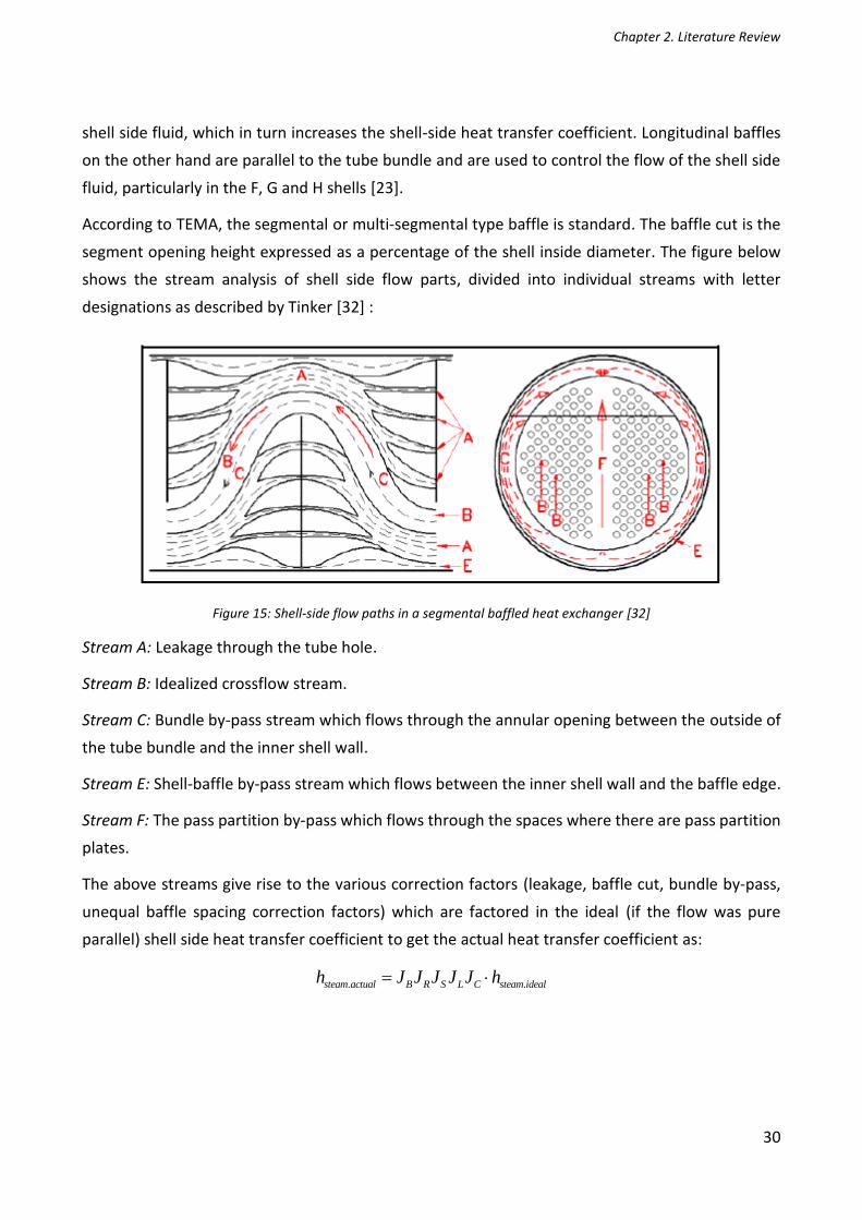
According to TEMA, the segmental or multi-segmental type baffle is standard. The baffle cut is the
segment opening height expressed as a percentage of the shell inside diameter. The figure below
shows the stream analysis of shell side flow parts, divided into individual streams with letter
designations as described by Tinker [32] :
Figure 15: Shell-side flow paths in a segmental baffled heat exchanger [32]
Stream A: Leakage through the tube hole.
Stream B: Idealized crossflow stream.
Stream C: Bundle by-pass stream which flows through the annular opening between the outside of
the tube bundle and the inner shell wall.
Stream E: Shell-baffle by-pass stream which flows between the inner shell wall and the baffle edge.
Stream F: The pass partition by-pass which flows through the spaces where there are pass partition
plates.
The above streams give rise to the various correction factors (leakage, baffle cut, bundle by-pass,
unequal baffle spacing correction factors) which are factored in the ideal (if the flow was pure
parallel) shell side heat transfer coefficient to get the actual heat transfer coefficient as:
. .steam actual B R S L C steam idealh J J J J J h=

Chapter 2. Literature Review
31
Where , , , &B R S L CJ J J J J are the bundle by-pass, laminar flow, unequal spacing, baffle leakage
and baffle cut correction factors respectively3.
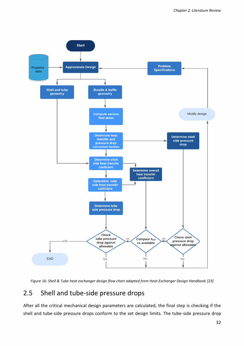
2.4.8 Detailed heat exchanger design process flow model
The detailed design of STHEs is briefly described in the flow chart below. The design process begins
with an approximate design which arrives at a tentative heat transfer area and physical design from
estimating the heat load and outlet temperatures. The most widely accepted approximate design
method is Bell’s Method [23]. After, that a more detailed design follows which takes into
consideration TEMA design guidelines and tolerances. Tube side design is quite standard as it
involves consideration of the tube side fluid, allowable tube-side pressure drops and then selecting
a suitable material to withstand the operating conditions of the tube side fluid.
Shell side design and performance on the other hand is quite rigorous due to the presence of shell
side constructional clearances (in the baffles and tube sheets) which cause fluid leakages, distorting
the perfect streamline flow of fluid [23] which has the net effect of reduction in heat exchanger
thermal effectiveness. Various methods have been put forward to determine shell side
performance, with the first flow distribution pattern being proposed by Tinker and later modified
by Palen et al [23]. This physical flow pattern was then used in the widely known and accepted Bell-
Delaware method for shell side performance [32] and then later modified by Taborek to account for
the shell-side heat transfer loss and additional pressure drops due to various leakages in the shell.
3 The equations for the stream leakage flow correction factors will be outlined in the mathematical model in Appendix B of this report.
Chapter 2. Literature Review
32
Figure 16: Shell & Tube heat exchanger design flow chart adapted from Heat Exchanger Design Handbook [23]
2.5 Shell and tube-side pressure drops
After all the critical mechanical design parameters are calculated, the final step is checking if the
shell and tube-side pressure drops conform to the set design limits. The tube-side pressure drop
Chapter 2. Literature Review
33
affects the pumping power requirement which in turn affects the auxiliary energy consumption.
According to the Indian Central Electricity Regulations Council, the allowable aux. power
consumptions for combined cycle thermal generating stations should be in the order of 2 – 5% for
thermal efficiency improvement [35].
Shell-side pressure drops, in this case has additional pressure drops due to cross flow, window zone
flow leakages, and end zone and nozzle inlet and exit losses, which will be calculated for the shell
side and added to the ideal pressure drop. The shell side pressure drop had to be kept as low as
possible to ensure the highest possible state at turbine inlet.
2.6 Feedwater heater structural design
An efficiency improvement to the basic Rankine cycle, shown in Figure 2 is using the low pressure
turbine steam (either exhaust steam or steam extracted after high pressure turbine expansion) to
preheat the feedwater, before it enters the economizer section of the boiler. In power plants, there
are two types of feedwater heaters: high pressure (HP) feedwater heaters situated after the
feedwater pump, and low pressure (LP) feedwater heaters located between the condenser and
feedwater tank [36]. In the HP feedwater heaters, the feedwater and the steam are not mixed, with
the normal construction being a shell and tube heat exchanger, with steam flowing in the shell and
feedwater in the tubes. For this reason HP feedwater heaters are also called closed feedwater
heaters. LP feedwater heaters can be closed or open, with the feedwater tank acting as an open
feedwater heater, responsible for both feedwater heating and removal of oxygen and carbon
dioxide gases (in the deaerator) which is necessary in feedwater chemistry control.
In the open feedwater heater, there is direct contact between the hot and cold fluids, with the
feedwater being sprayed into the tank and the LP steam bubbled from the bottom of the feedwater
tank, mixing with the feedwater and exchanging heat until thermal equilibrium is reached. The HP
heaters after the feedwater tank are also closed feedwater heaters, with large power plants typically
employing 3-4 LP feedwater heaters and 3 -5 HP feedwater heaters [36]. Optimum placement of the
HP feedwater heaters begins by defining the enthalpy difference between the feedwater pump and
the economizer inlet, then dividing it by the number of HP feedwater heaters, giving the enthalpy
rise in each HP feedwater heater stage [36].
2.7 Steam turbines and application to small steam plants
The steam turbine is a heat engine which transforms thermal energy from pressurized steam to
kinetic energy by flow through nozzles, which is then converted to a force doing work on rings of
blading mounted on a shaft [37]. It is used for various industrial operations, mostly power
Chapter 2. Literature Review
34
generation and providing mechanical work to drive process equipment like pumps and fans. The
first practical turbine was made by C. Parsons in 1884 and the usual turbine consists of four
fundamental parts:
• Rotor – shaft which carries the blades or buckets,
• Stator – also known as the cylinder or casing within which the rotor turns and where the
nozzles are fixed,
• Nozzles – which direct the steam on the rotor blades,
• Frame/ base – for supporting the turbine assembly.
The energy conversion process in the steam turbine is from potential (high pressure) and thermal
(temperature) energy in the steam, to kinetic energy (acceleration in the nozzle) and then rotational
energy (torque and speed) in the rotor shaft.
Classification of steam turbines is done in various ways [37]:
i. w.r.t form of blade passage – impulse, reaction or combination impulse and reaction turbine.
ii. w.r.t internal design and flow sequence - single flow, double flow, divided flow, compound
flow etc.
iii. w.r.t direction of steam flow relative to plane of rotation – axial, radial or tangential flow.
iv. w.r.t rotational speed – for 60 cycle or 25 cycle generators and for geared units without
special speed requirements.
v. w.r.t conditions of use – reheat, extraction, back pressure, regenerative or mixed pressure
turbines.
vi. w.r.t passes of steam flow through blades – single pass or re-entry turbines.
In this section, more literature will be covered on classification of steam turbines with respect to
conditions of use to enable the selection of a suitable turbine for the operating conditions required.
2.7.1 Classification of steam turbines w.r.t conditions of use
This classification places emphasis on the boundary conditions of the steam at both turbine inlet
and exit, focusing on:
• Inlet pressure – high, intermediate, or low-pressure turbine.
• Exhaust condition – condensing, non-condensing or back pressure, extraction-condensing
turbine.
• Steam mass flow through the turbine – extraction, regenerative or reheat turbine.

Chapter 2. Literature Review
35
Condensing turbine
The condensing turbine exhausts steam at below atmospheric pressure to allow it to be condensed
to liquid water in the condenser. It is employed in power plants where the requirement is power
only and thus all the steam which enters the turbine is exhausted at the exit stage (assuming no
leaks or extractions).
Non-condensing/ Back-pressure turbine
In the non-condensing turbine, the steam is exhausted at low pressure but above atmospheric,
usually between 1-12bar. It is mostly employed in process plant industries where there is both a
power and process steam requirement. In this set-up, the condenser is removed, and the process
plant acts as the “condenser” whilst utilizing the heat in the exhaust steam for process heating.
Extraction- condensing turbine
In this turbine, part of the steam is bled/ extracted at the process pressure requirements and the
remaining steam is further expanded in the low-pressure turbine stages and finally condensed in
the condenser.
High pressure (HP) turbine
Usually employed in utility power plants, where operating pressures are high and receive high
pressure, high temperature steam (main steam) from the boiler. The HP turbine can be condensing
or non-condensing. High pressure condensing turbines exhaust at below atmospheric pressure and
large volume [37] thus are designed to have short blading at the HP end and long blading at the low
pressure (LP) end.
High pressure non-condensing turbines on the other end exhaust steam at moderate steam
conditions for use in factory processing or heating applications. They are also used in instances
where cooling water for condensing is unavailable and are built in small or moderate sizes [37].
Intermediate pressure (IP)/ Reheat turbine
The intermediate pressure turbine is usually placed between the high- and low-pressure turbines.
It receives the HP turbine exhaust as its input steam and exhausts to the LP turbine inlet. It is
however mostly known as the reheat turbine, because the turbine does not receive the HP exhaust
Chapter 2. Literature Review
36
directly from the HP turbine, but from the boiler reheaters. After expansion in the HP turbine, the
HP exhaust is sent to the boiler reheater tubes located usually between the platen and pendant
superheaters, at HP exhaust pressure and reheated to the main steam temperature. After that, the
steam is then returned to the IP turbine to complete its expansion before subsequent exhaustion
into the LP turbine. Such arrangements are generally only found in power generation plants.
Low pressure (LP)/ Exhaust turbine
The low-pressure turbines are usually the last stages of expansion before condensing. They are
employed in applications where large power output (hence large mass flow) is required in a single
machine [37]. In order to control the length of the turbine and avoid turbine vibrations, the HP and
LP stages are divided into separate casing, having a separate LP turbine. There are also very often
more than one LP turbine running in parallel for a single HP turbine due to the large volume flow
requirement at the exhaust. The LP turbine is designed to handle high volume, low pressure, and
lower quality steam at the final stages.
Mixed pressure turbine
The mixed pressure turbine is designed to handle two different steam pressures. It can be HP-LP/
IP-LP combination, or two different LP inlets and the low-pressure inlet is usually from another heat
engine or turbine e.g., gas turbine combined cycle plants. This turbine is thus more employed in
applications where it is desirable to recover waste heat from other heat engines for power
generation. The LP steam joins the HP steam after it has been expanded down to the pressure at
which LP steam is usually received at.
Regenerative or bleeder turbines
The regenerative turbine receives HP steam at inlet, and at one or more stages before the steam
has been exhausted to its final low pressure, it is bled / withdrawn at intermediate pressures for
feedwater heating [37]. The feedwater is heated in stages with the last feedwater heating occurring
at the highest temperature bled steam. Regenerative turbines are almost similar in principle as the
extraction-condensing turbine except the extraction turbine steam goes to the process not feed
water heaters.
In this study, the maximum pressure is 950kPa, and the steam is required to be exhausted at 400kPa
to meet process plant demands. The suitable turbine for this operation is thus a back-pressure
turbine which can operate in the low-pressure ranges. Important to note, in addition to knowing

Chapter 2. Literature Review
37
the turbine operating conditions it is important to know how the steam changes state from turbine
inlet to exhaust. This is done on the Mollier diagram, using a turbine expansion line.
2.7.2 Turbine Expansion Line
Figure 17: Typical turbine condition line
Also known as the condition line, the turbine expansion line (shown above), depicts the thermal
state of the steam as it expands through the turbine. Steam enters the governing valve at state point
th, where the pressure is reduced due to valve losses to point 0. From point 0 – 1, the flow is
accelerated in the nozzle but due to nozzle losses, the flow is shifted from the ideal lossless exit
enthalpy at 0s to state point 1. In each turbine stage, the rotating blades extract a portion of the
flow’s kinetic energy (depicted as the red vertical bars), and the remainder moves on to the next
stage. At entry to the next stage, some kinetic energy is lost due to carryover losses. This further
shifts the steam state to point 1x where it has lower inlet velocity at entry to stage 2.
The carryover losses, also known as leaving-velocity losses occur between stages because of the
difference in the stage diameters or when there is a huge axial space between adjacent stages. It is
high in the governing and the exhaust stages because of the formation of eddies between the nozzle
and moving blades and also since there is no further device to extract kinetic energy after the last
stage. This heat loss which is not extracted as useful work, but raises the total heat and entropy of
the steam from point 1 to point 1x is also known as reheat as it appears like more heat has been
added to the steam between stages which can be seen in Figure 17 above. The more the number of
stages, the more these “inter-stage reheats” are, which increases the turbine’s reheat factor.

Chapter 2. Literature Review
38
However, for any specified initial steam conditions, final pressure and stage efficiency, there is a
limiting value of the reheat factor which corresponds to an infinite number of stages and for any
finite number of stages, the reheat factor will be less [37].
At point 4, all the unused kinetic energy is lost at outlet to point 5. The enthalpy at point 4 and 5 is
known as the expansion line end point (ELEP) and used energy end point (UEEP) enthalpy
respectively. The blue line is the condition line of the turbine.
2.7.3 Turbine efficiency
Turbine efficiency is a measure of how well the turbine converts the input heat into mechanical
work. It is determined by considering the actual work output to the maximum possible work which
could be extracted by the turbine. The maximum work is only realized when there are no losses,
which is represented by the ideal isentropic line (0 - s) between the inlet and outlet on Figure 17
above. The actual turbine work is depicted by the condition line from the turbine inlet to the UEEP
and thus the efficiency is calculated as:
0 5
0
turbine
s
h h
h h
−=
− (2.30)
A Siemens SST-060 turbine alternator was selected as the suitable turbine to convert the thermal
energy in the superheated steam from the heat exchanger, to mechanical work and electrical
energy. This decision was arrived at basing on information acquired from previous research done by
the researcher in an undergraduate project.
2.7.4 Siemens SST-060 Turbo-Alternator set
Siemens Turbomachinery Equipment (STE) has a range of small-scale turbine technologies, with four
distinct product lines: the SST-050 (up to 750kW), the SST-060 (up to 5000kW), the SST-110 (up to
7 000kW and the SST-120 (up to 10 000kW) with basic technical values as follows:
• Live steam pressure: 3 - 131bar (absolute),
• Live steam temperature: Dry saturated – 530˚C,
• Exhaust steam pressure: 0.08 – 29bar,
• Speed: 500 – 23000rpm,
• Power: Up to 10 000kW.
Through consultation with the Siemens team, the SST-060 was recommended as the most applicable
set for this duty.

Chapter 2. Literature Review
39
Figure 18: Siemens SST-060 Turbo-alternator set
Previously known as the “Dampfturbine”, the SST-060 (shown above) was originally designed and
manufactured by Kuhnle, Kopp & Kausch AG, a company established in 1899 which was later
acquired by Siemens in 2007. The turbine range has a modular design which allows it to be
connected in different combinations, making it very flexible and able to meet a wide range of
customer specifications [38].
It is a predesigned radial inflow impulse turbine, which has many applications and can be ordered
as a standalone unit (without generator) for use in mechanical drivetrains or as a turbo-alternator
for power generation in cogeneration, biomass, waste-to-energy, and heat recovery generator
projects [39]. The turbo-alternator can be used as both a backpressure or condensing turbine, with
an integral cooling system. It can operate smoothly through its range of operating speeds up to
overspeed. The figure below shows the detailed specifications of the SST-060 unit.
Rotor blade – CFR type
Nozzle ring

Chapter 2. Literature Review
40
Figure 19: SST-060 Specifications [39]
The researcher used the Siemens option as it was the only manufacturer with easily accessible
literature on the small-scale turbines and has been referenced in many cogeneration webinars like
the International Energy Agency Bioenergy Task 32 and 33 [39]. Siemens is a well-known turbine
manufacturer with years of providing quality and reliable turbines. Another factor which made the
SST-060 a turbine of choice, is the fact that it is suitable for quick start without preheating, making
it ideal for a SAPG system which has an intermittent heat supply source for the main steam.
2.8 Steam plant economics
One of the most important aspect of project evaluation is assessment of profitability or cost
effectiveness. Power plant projects are mostly must-have capital intensive investments [40], whose
investment appraisal focuses on minimizing costs (least cost approach) rather than maximizing
profit. Where the power plant project is state-owned, the economic viability is measured based on
levelized cost of energy rather than payback period. Capital for these projects is government
sourced, and the investment is paid back from tax revenue, unlike in independent power producer

Chapter 2. Literature Review
41
scenarios where the projects are private investor owned and the narrative shifts from just
minimizing costs but ensuring a positive return on investment in the shortest possible time.
In this research, the researcher adopted the discounted payback period to check the profitability of
the project. Despite there being other widely used and accepted methods of evaluating project
profitability (net present value or internal rate of return), the discounted payback method was
selected because for an already operational food and beverage processing industry whose key
objective is food processing, focus is on how soon the CAPEX can be recouped than other
profitability indicators like the net present value. The important factor to consider in this
augmentation is at what cost and how long it takes to recoup the initial investment rather than cost
of energy. The total capital investment was calculated based on the procedure outlined below.
2.8.1 Primary equipment
The capital investment of the project is largely influenced by the turbine capital costs, size of solar
field required to meet the thermal heat addition and heat exchanger cost. The turbine costs were
obtained from the manufacturer in 2016, shown in Appendix D of this research. Efforts to obtain a
more recent quote did not yield any positive results as manufacturers only release accurate cost
data to customers with orders. However, the initial quote was in Euros and the variation in exchange
rate of the Euro:US$ in the past 5 years is not that big and will be accounted for in the sensitivity
analysis rather than trying to refine cost estimates which is beyond the scope of this study.
Solar system costs will be done using the SAM NREL system advisor model costing template which
is based on actual United States Department of Energy’s National Renewable Energy Laboratory
(NREL) past project’s cost data. The SAM financial model is also based in US$ and variations in the
exchange rate between the US$ and the ZAR will be used in the sensitivity analysis to account for
the time value of money.
2.8.2 Heat exchanger costs
Critical in this study is designing a heat exchanger to superheat the saturated steam of the boiler,
thus estimation of the manufacturing cost of the optimum design is a major concern. Cost
optimization of heat exchangers, particularly shell and tube heat exchangers has been an ongoing
process, with parametric methods or variant based costing being the most popular [41]. The
parametric costing models rely on heat transfer area as the base factor to calculate total heat
exchanger cost and uses an exponential equation to calculate direct manufacturing cost, such as the

Chapter 2. Literature Review
42
formulation of Hall [42]. To increase the accuracy of the result, application (pressure factor) and
structural (length of tubes) coefficients are also included.
However, the parametric estimates are based on a specific heat exchanger configuration, provide a
purchasing cost which is affected by market situations and limited to a range of heat exchanger sizes
(e.g., Hall’s formulations are limited to heat transfer areas below 140m2) [41]. This has led to the
development of generative cost models which allow for up-to-date cost estimates, which reflect the
effect of design variations on the manufacturing costs. The equations used to calculate the heat
exchanger cost were adapted from the works of Caputo et al. [42] and will be presented below.
Direct manufacturing cost of a heat exchanger is the sum of materials and manufacturing processes
cost:
, , ,
1
n
m x mat x op k
k
C C C=
= + (2.31)
where ,m xC is the manufacturing cost of the xth component of the heat exchanger;
,mat xC is the
material cost, n is the number of processes needed for each component of the heat exchanger and
, op kC is the cost of the kth operation on the xth component .
The material cost of the xth component:
,mat x x x matC V C= (2.32)
where V is volume in m3, x is the density in 3
kg
m and matC is the material cost in ZAR.
The cost of the kth operation on the xth component:
, ,
kop k H k
k
LC C
v
=
(2.33)
Where L is the manufacturing process length, v is the operation speed and HC is the hourly rate.
However, the detailed cost of processing includes summing up the labour, consumables and
equipment amortization which is beyond the scope of this research. For simplicity’s sake, the
manufacturing cost was estimated as 50% of the total material cost and would be included in the
sensitivity analysis if it was found to play a major role in the overall costing. The eventual
component cost equation therefore reduced to:
, 1.5m x x x matC V C= (2.34)
Chapter 2. Literature Review
43
2.8.3 Total capital investment
Total capital investment is the amount of money required to install the system. It includes the total
heat exchanger cost, steam turbine cost and solar system capital costs. This will be the loan amount
which will be used to calculate of the discounted payback period, using the energy savings obtained
by operating the power generating system when the solar resource is available during the day.
/turb sf H ELoan C C C= + + (2.35)
Where turbC , sfC and
/H EC are the turbine, solar field and heat exchanger capital costs respectively.
The cost of process control e.g. isolation valves, control valves, safety valves, modulators,
instrumentation and distributed control system integration could potentially cost as much as the HX
but due to scope of this study will not be included. Impact of HX cost variation will be studied in the
sensitivity analysis.
2.8.4 Payback period
Payback period is the time required to recover the costs incurred in an investment. The ordinary
payback period is calculated by dividing the initial capital outlay with the estimated periodical net
cash flows. Where the time value of money is considered, by considering loan interest rates, it is
called the discounted payback period. This is particularly of interest to the investor as it gives an
insight on how long it will take to recoup the initial capital investment of the project. In this study,
the annuity equation was used to derive the discounted payback period formula. The annuity
equation states that:
1 (1 )n
Loan rA
r
=
− + (2.36)
Where A is the yearly / monthly fixed instalment to be paid back to recoup the initial loan
investment over a predetermined period n and r is the interest rate per period. It is however
advisable to pay back the instalments in the shortest possible time as each instalment reduces the
balance on the capital, subsequently reducing the interest payable. By making n the subject of the
formula, the discounted payback period can be calculated as shown in (2.37) below:

Chapter 2. Literature Review
44
12ln 1 ln 112
12
months
rLoan
rDPP
CF
= − +
(2.37)
Where monthsDPP is the discounted payback period in months, r is the interest rate per annum and
CF is the annual cash savings made by producing energy at the site, calculated as:
,( )annual produced OPEXCF E Tariff C= − (2.38)
Where,annual producedE is the electrical energy produced per annum and
OPEXC is the annual operating
and maintenance costs of the system.
2.9 Conclusion
The literature reviewed in this chapter will be the backbone for the model development and system
design that form part of this thesis. The first section looked at the process steam plant basics,
focusing on the process steam plant thermodynamic cycle and how it is related to the conventional
power plant cycle. The next section looked at cogeneration and how a basic steam plant can be
retrofitted to enable the generation of both heat and power by adding additional heat into the
system. Section 2.3 looked at solar thermal plants, which will be used to provide additional heat to
superheat the steam from the boiler and the next section focused on the design of the superheater.
Steam turbines were briefly discussed as they are the heat engines responsible for converting the
thermal energy to mechanical work. The last section looked at steam plant economics as this gives
the measure of economic viability of undertaking such a project to both the researcher and potential
investors.

Chapter 3. Methodology
45
3. Methodology
3.1 Model Investigation
In this section of the report, the findings of the qualitative component of this research which were
used in the development of ideas for the quantitative research are presented. A number of site visits
were done to food and beverage processing industries with the capacity to install combined heat
and power systems, as well as those which already have such systems in place, to gather information
on how their current systems are working. In addition to that, the researcher visited a local steam
boiler manufacturing company to learn more about steam boiler design.
3.1.1 Research Questions
The research questions were broken down into three distinct groups: questions on boiler design,
questions on process plants with the potential to adopt Cogeneration, and those for plants with
Cogeneration already in place. Outlined below are the different research questions:
3.1.2 Boiler Design Questions
▪ Can an existing fire-tube (package) boiler be retrofitted to produce superheated steam?
▪ What are the design considerations to be made when retrofitting a package boiler?
▪ What is the effect of exceeding the maximum continuous rating of a boiler, especially on the steam
release rate?
3.1.3 Process Steam plants
▪ What is the maximum plant electricity demand?
▪ What is the capacity of the existing process plant?
▪ Which processes require process steam in the operation and at what temperature and pressure?
3.1.4 Existing Combined Heat & Power Plants
▪ How is the cogeneration system currently working?
▪ What is the plant process thermal load requirement?
▪ Is power generation driven by the thermal load or electrical load?
▪ How are fluctuating demands, in terms of both thermal and or electrical load managed?
▪ Was the system originally designed for Cogeneration or was it upgraded to one? If yes, what were
the considerations made in the upgrade?

Chapter 3. Methodology
46
After drawing down the relevant questions for each section of the research, document analyses,
interviews, and observations were used to provide answers to the questions at the sites which were
visited. The data obtained provided the basis of the quantitative aspect of the research.
3.2 Site visit reports
3.2.1 John Thompson Boilers
John Thompson boilers, a division of ACTOM Private Limited manufactures electro-mechanical
equipment (package boilers, water-tube boilers, utility boilers) largely used in the steam plant
industries. The visit to John Thompson was meant to answer questions on the design considerations
to be made when retrofitting a package boiler to produce superheated steam and effects on boiler
operation.
Package Boiler Retrofit
It is possible to convert an existing package boiler to superheat steam for power generation.
However, the design of Fire-tube boilers is governed by BS EN 12953:3 which outlines specific
tolerances and design standards. At John Thompson, the superheater is fitted on the smoke box and
boilers in service can be sent back for the retro fitment. Boiler energy efficiency can be analysed on
three different levels:
▪ Boiler thermal efficiency - how well the boiler transfers heat?
▪ Combustion efficiency - ability of the burner to completely use the energy in the fuel without
generating carbon monoxide or leaving hydrocarbons unburned.
▪ Fuel-steam ratio.
When making any changes to the boiler, one should take into cognizance that the pressure rating
cannot be changed as it is proportional to material thickness and composition. The boiler is
approved by a third party and certified by the department of labor based on the pressure, steaming
rate and fuel fired. If any of these parameters change, the boiler will have to be re-certified.
In addition to that, further questions came up from this visit:
▪ How does preheating the feedwater with an external energy source affect the boiler firing
rate and flue gas flows?

Chapter 3. Methodology
47
It was noted that preheating the feedwater with an external thermal energy source like solar power
will reduce the mass flow rate of coal, lowering the flue gas fumes. This reduces the boiler’s carbon
footprint.
3.2.2 Kadoma Paper Mills
Kadoma Paper Mills manufactures tissue and craft products from recycled wastepaper. The recycled
paper is sorted, graded, and pulped to manufacture different grades of paper (enhanced white
tissue, hand towelling tissue, tinted tissue and craft paper).
Existing Steam Plant Specifications
Kadoma Paper Mills has four fire-tube boilers: three rated at 4.5 tonnes per hour (tph) and one
rated at 3.5tph used for process steam generation. The steam is generated at between 10 and 12bar
and used mainly on their M.G. Cylinder (tissue making machine) for paper drying, pulping, and
preheating processes around the plant. Currently, one 4.5tph boiler is enough to run the whole
plant as their second section which was the largest was decommissioned following the economic
decline in Zimbabwe. The current maximum electrical power demand is 741kW.
Thermal Load Specifications
The table below outlines the process steam requirements at Kadoma Paper Mills:
Table 1: Kadoma Paper Mills Process Steam Requirements
Process Temperature [T - ˚ C] Pressure −P kPA Dependence
Paper drying 110-150 (Off-take)
140 (Boiling)
540
500 T, P
Pulping 50 300 P
3.2.3 Tongaat Hulett Triangle Zimbabwe
Triangle Limited is an Agri-based industry that produces a variety of sugar products (raw, brown,
and white sugar) from sugarcane. The diagram below shows the process flow at Tongaat Hulett:

Chapter 3. Methodology
48
Figure 20: Tongaat Hulett Triangle Process Flow Diagram
The process inputs are cane, which is processed to produce cane juice and waste known as bagasse.
All the plant electrical power needs are met with a steam turbine topping power plant, which uses
the waste bagasse as the fuel source.
Existing Steam Plant Specifications
Tongaat Hulett began operations in 1931 when the first sugar plantation was planted. Processing
was done much later in 1939 and old mills from their sister company in South Africa were used. In
the late 1960s, as the business grew, it was decided to relocate to where the current mill house is
and that is when the power plant was also set up to meet the demands of their large equipment
(the shredder alone is rated at 1.8MW). Steam turbines and auxiliary equipment were bought from
Hwange Power Station as they were upgrading their plant and the boilers from John Thompson.
From the look of the current setup, the plant was designed for Cogeneration from the onset to
provide for both the process plant steam needs and plant power demand.
Currently four boilers are in operation: Boiler 7 & 8 rated 45tph each, Boiler 9 rated 100tph and
Boiler 10 rated 150tph. Steam is generated in the boilers at 3.2MPa and at 370˚C when using coal
as fuel and 390˚C when using bagasse as fuel. The main fuel source is bagasse which is obtained
from the cane extraction plant at 50% moisture. Coal is mainly used as a supplement during start-
ups, breakdowns, and routine maintenance in the extraction plant. The maximum plant steam

Chapter 3. Methodology
49
demand is 250tph and varies as the cane fed varies. Main steam is sent to the steam turbines for
power generation.
The total installed capacity is 32.5MW, with five back pressure and one condensing steam turbine
(TA2). All turbines are impulse type axial flow steam turbines rated as follows: TA1 - 6MW, TA2 –
3MW, TA3 – 2MW, TA4 – 6MW, TA5 - 8MW and TA6 -7.5MW. The backpressure turbines exhausts
at 130 ± 10 kPa and 120 ± 5˚C, and the exhaust steam is sent to the factory for heating and drying
purposes. Below is a steam and condensate flow diagram detailing how the steam flows in the
system:
Figure 21: Tongaat Hulett Triangle Steam & Condensate Flow Diagram
The condensing turbine was left out of the flow diagram as only one turbine was made
representative of the four back-pressure units. It is only used momemtarily when the steam flow is
more than the process thermal load requirement. The ideal operating scenario is to ensure that the
mass flow into the turbine matches the process plant steam requirement. Where the mass flow into
the turbines exceeds the process plant requirement, some of the steam is condensed whilst
decreasing the boiler firing rate to match thermal load requirement. This will be explained further
in the System manipulation section.

Chapter 3. Methodology
50
System Manipulation
In-order to manage fluctuations in both the thermal load and plant power demand, the following is
done:
If the thermal load increases beyond the capacity of the steam coming from the turbine exhaust,
live steam is bled from the boilers and passed through pressure reduction drag valves where the
pressure is reduced to 150kPa and sent to the process. When the thermal load falls below what the
turbines are producing, the exhaust steam is condensed and at the same time the boiler firing rate
is reduced to match turbine exhaust with the process steam requirements. Excess bagasse is
stockpiled for use when the thermal load spikes up.
When the electrical load increases above the power generated when operating in island mode (off-
grid), the system is synchronized with the 6.6kV busbar and set to import from Zimbabwe Electricity
Supply Authority (ZESA). On the other hand, when the turbine-alternators produce more than the
plant electrical demand when operating in island mode, the turbine-alternators are synchronized
with the 6.6kV bus bars and export to the grid momentarily whilst the boiler feed rate is lowered to
match generation with plant electricity demand. Tongaat Triangle, unlike Tongaat Hulett Hippo
Valley Estates does not have a contract with ZESA to sell its excess to the Power Distribution Utility.
In that case, any energy exported by Triangle Limited is free of charge thus the ideal operation
scenario is to just produce electricity enough to meet their own needs.
3.2.4 African Distillers
African Distillers manufactures, distributes, and markets under license, branded wines, spirits, and
ciders for both the local market and beyond. Situated in Mt Hampden, about 30km west of Harare’s
central business district, African Distillers (AFDIS) has six depots in Harare, Bulawayo, Kwekwe,
Mutare, Victoria Falls, and Masvingo, supplemented by customer collection depots countrywide.
Existing Steam Plant Specifications
AFDIS has three coal fired fire-tube boilers: two 4.5 tph boilers and one 2.5 tph boiler, which are
currently used for process steam generation. The steam is generated at between 600 and 850kPa
and used in the blending and bottling departments for distillation, pasteurization, cleaning in place
(CIP), bottle washing, and bottle warming. Plant maximum electrical power demand is 621.28kW.

Chapter 3. Methodology
51
Thermal Load Specifications
Table 2: African Distillers Process Steam Requirements
The location for conducting the research was largely selected based on the available infrastructure
for setting up a combined heat and power plant, ease of access to plant data and scale of production
from the three sites visited by the researcher namely Kadoma Paper Mills, African Distillers and
Tongaat Hulett Triangle Limited. Tongaat Hulett was ruled out as it already has Cogeneration in
place and based on the criteria, the best site for the project was identified as African Distillers
(AFDIS) Private Limited.
3.3 Model development
The next step after site selection was coming up with a feasible process layout for the new system,
considering different arrangements and design considerations. The design concepts are briefly
described in the subsequent section.
Process Temperature [T - ˚ C] Pressure −P kPA Dependence
Distillation 75-78 (Off-take)
95-98 (Boiling) 350 T, P
Pasteurization 72.3-80 400 T, P
Cleaning In Place (CIP) 80 400 T, P
Bottle Washing 90 - T
Bottle Warmer 28-30 - T
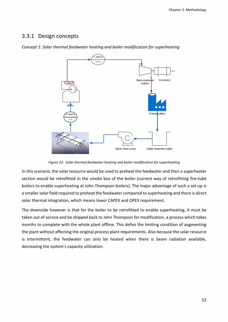
Chapter 3. Methodology
52
3.3.1 Design concepts
Concept 1: Solar thermal feedwater heating and boiler modification for superheating
Figure 22: Solar thermal feedwater heating and boiler modification for superheating
In this scenario, the solar resource would be used to preheat the feedwater and then a superheater
section would be retrofitted in the smoke box of the boiler (current way of retrofitting fire-tube
boilers to enable superheating at John Thompson boilers). The major advantage of such a set-up is
a smaller solar field required to preheat the feedwater compared to superheating and there is direct
solar thermal integration, which means lower CAPEX and OPEX requirement.
The downside however is that for the boiler to be retrofitted to enable superheating, it must be
taken out of service and be shipped back to John Thompson for modification, a process which takes
months to complete with the whole plant offline. This defies the limiting condition of augmenting
the plant without affecting the original process plant requirements. Also because the solar resource
is intermittent, the feedwater can only be heated when there is beam radiation available,
decreasing the system’s capacity utilization.

Chapter 3. Methodology
53
Concept 2: Direct solar thermal integration with super-heating
Figure 23: Direct solar integration for superheating
Direct integration of the solar thermal system with the existing process plant involves feeding the
boiler exit saturated steam into the solar thermal field as shown in Figure 23 above. In this system,
less solar field system components are required as direct superheating of steam can be done, which
also lowers the CAPEX and OPEX requirement. The major disadvantage however is that due to the
daily variation of the solar resource there are instances when the system, instead of adding heat to
the dry saturated steam from the boiler, will be extracting heat from it, lowering system efficiency.
In addition to that this might imply frequent turbine trips, when the steam quality at turbine inlet
does not meet the turbine boundary conditions, and poor process temperature control.

Chapter 3. Methodology
54
Concept 3: Indirect solar thermal integration with super-heating
Figure 24: Indirect solar thermal integration with superheat
For better temperature and pressure control, which is of critical importance at the turbine inlet,
indirect integration becomes a better option as a separate heat exchanger is used to heat the steam
using the solar thermal energy. The downside however for this set-up is increased capital and
operating costs as there are more system components. In addition to that, exhausting at the process
pressure implies superheated steam is exhausted at the turbine exhaust stage because of the low
operating pressure of the turbine. This calls for the use of a de-superheating mechanism like the
direct spray type shown above. The desuperheater introduces cold feedwater to the exhaust steam
and it cools it down to dry saturated state before it is piped to the process.
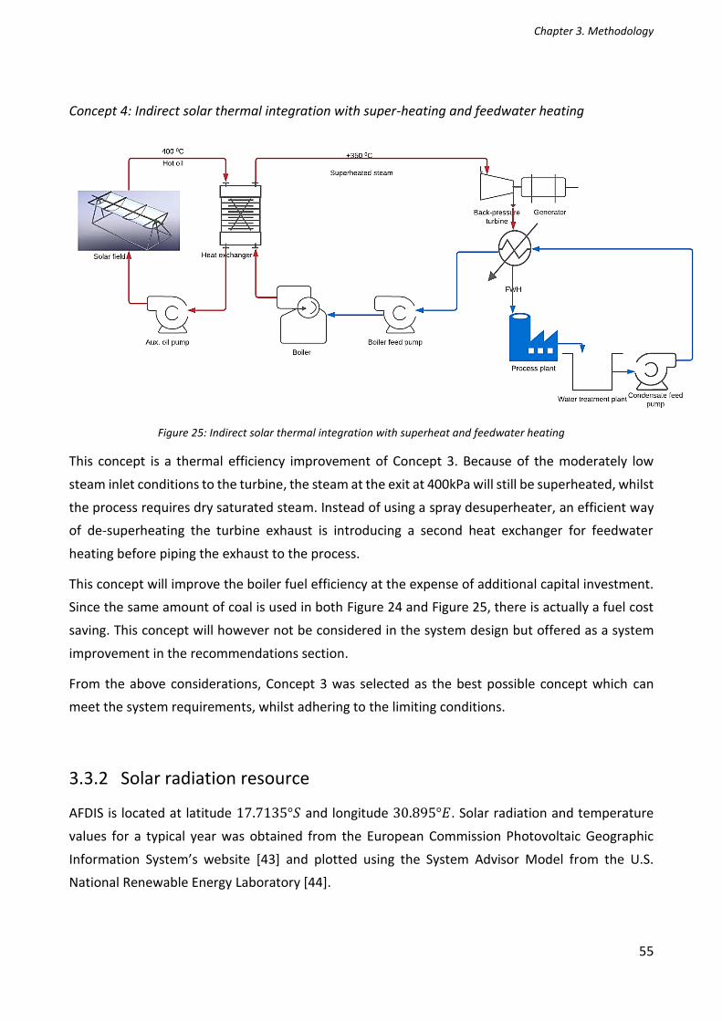
Chapter 3. Methodology
55
Concept 4: Indirect solar thermal integration with super-heating and feedwater heating
Figure 25: Indirect solar thermal integration with superheat and feedwater heating
This concept is a thermal efficiency improvement of Concept 3. Because of the moderately low
steam inlet conditions to the turbine, the steam at the exit at 400kPa will still be superheated, whilst
the process requires dry saturated steam. Instead of using a spray desuperheater, an efficient way
of de-superheating the turbine exhaust is introducing a second heat exchanger for feedwater
heating before piping the exhaust to the process.
This concept will improve the boiler fuel efficiency at the expense of additional capital investment.
Since the same amount of coal is used in both Figure 24 and Figure 25, there is actually a fuel cost
saving. This concept will however not be considered in the system design but offered as a system
improvement in the recommendations section.
From the above considerations, Concept 3 was selected as the best possible concept which can
meet the system requirements, whilst adhering to the limiting conditions.
3.3.2 Solar radiation resource
AFDIS is located at latitude 17.7135°𝑆 and longitude 30.895°𝐸. Solar radiation and temperature
values for a typical year was obtained from the European Commission Photovoltaic Geographic
Information System’s website [43] and plotted using the System Advisor Model from the U.S.
National Renewable Energy Laboratory [44].

Chapter 3. Methodology
56
Figure 26: AFDIS GHI and dry bulb temperature annual variations from SAM NREL
The global horizontal irradiance (GHI) is the total solar radiation incident on a surface. It is the sum
of the direct and diffuse component of radiation incident on a surface and is a measure of the total
available solar thermal energy which can be harnessed. In CSP projects, the important component
is the beam radiation (direct normal irradiance). The design point DNI for the site is 920 𝑊𝑚2⁄ .
Temperature data is the dry bulb temperature and is very important to consider when selecting the
solar heat transfer fluid which is best suited for the site’s weather conditions.
3.3.3 System Design Inputs
System boundary conditions are the boiler outlet steam properties (which will be the cold fluid inlet
conditions in the heat exchanger) and the process thermal load requirements (which will be the
turbine exhaust conditions). Additional data is the plant power demand which will dictate the size
of superheater. The heat input need not exceed the power requirement. However, it is possible
that due to other limitations, it may not be possible to achieve the total required heat input. The
actual heat exchanger thermal load will be an input to the external solar field sizing, as the field
need only be as big as the heat that can be transferred in the heat exchanger. The table below
summarizes the key system design inputs:

Chapter 3. Methodology
57
Table 3: System Boundary Conditions
Parameter Value
Steam mass flow 2.5 kg/s
Boiler outlet 950 kPa, x=1.0
Turbine exit 400 kPa
Electrical load 622 kW
Process input 100 °C, 350 kPa
3.3.4 Heat Transfer Fluid Selection for the Solar Field
The key decision factors in selecting the suitable heat transfer fluid for the solar field are briefly
discussed below.
• Heat capacity: Temperature change is inversely proportional to the heat capacity. Fluids with
a higher heat capacity need a lot of heat to be added before a significant temperature
change is noted and vice versa. An ideal heat transfer fluid should have a high heat capacity
to be able to store as much heat energy as possible.
• Thermal stability: Certain oil based HTFs can significantly degenerate at elevated
temperatures thus the operating temperature range should be below the temperature the
HTF degenerates.
• Solidification temperature: The ideal heat transfer fluid should have a freezing point lower
than the site’s minimum temperature to avoid in service solidification which leads to blocked
piping.
• Evaporation temperature: This is the thermal stability limitation. The HTF should have a high
evaporation temperature at low pressure to avoid flashing in service.
• Thermal conductivity: High thermal conductivity to ensure the receiver temperature is as
close as possible to the heat transfer fluid temperature.
• Viscosity: The higher the HTF viscosity, the greater the pumping power required to pump the
fluid in the system. Ideal HTF should have low viscosity to minimize plant auxiliary power
requirement.
• Density: The HTF should have a high density to enable its use as a storage medium.
• Toxicity and environmental hazards: Easy to dispose and non-toxic heat transfer fluids are
preferred to avoid damaging the environment and posing health risks to plant personnel.

Chapter 3. Methodology
58
• Corrosivity: A corrosive fluid leads to higher operational costs due to frequent heat
exchanger piping replacement. An ideal fluid should be non-corrosive.
• Explosivity: For safety of both plant and personnel, the ideal HTF should be non-explosive.
The table below shows the key thermophysical properties used in the selection of the heat transfer
fluid:
Table 4: Heat Transfer Fluid selection decision table [31], [45]
HEAT
TRANSFER
FLUID
Specific heat
capacity
kJ
kgK
Max temp
( )
Min temp
( )
Kinematic viscosity
@ 100˚ C
Market popularity
Therminol VP-1 2.889 400 12 0.99 Popularly used
DowthermTM A 2.4093 400 15 0.91 Popularly used
Hitec Salt 1.56 538 149 -
Still in the
developmental phases
• The heat capacity of a fluid is its ability to absorb heat relative to its change in temperature.
• Maximum operating temperature is the maximum attainable temperature of the HTF and
the higher the maximum temperature, the more favourable the HTF for use in the heat
exchanger.
• Minimum temperature is the limit the HTF can operate without change in state or physical
properties. The lower the minimum temperature, the lower the freeze point and the more
favourable the HTF for low ambient temperature conditions
• Viscosity is the measure a fluid’s resistance to flow, the more viscous the fluid, the difficult
it is to flow. An ideal HTF should have less resistance to flow to avoid clogging and fouling of
the heat exchanger.
• The more popular a HTF is on the market, the ease of availability of both the HTF and all the
necessary in-service data.
Therminol VP-1 was selected as the final heat transfer fluid because of its higher heat capacity and
popularity in the market as a HTF. Although the molten salt has more favourable properties, its use
in the solar thermal systems is still in the development phase.

Chapter 3. Methodology
59
3.3.5 Heat exchanger approximate design
The detail calculations for the approximate design can be found in Appendix A. The flowchart below
outlines the process and is followed by a brief explanation of the steps.
Figure 27: Heat exchanger approximate design flow chart [23]
Step 1: Fluid flow allocation and fluid boundary condition properties calculation
For the heat exchanger design, the heat transfer fluid, being the higher fouling fluid was placed in
the tube-side and the steam in the shell. Using the Therminol Fluid properties calculator [31], the
heat transfer fluid inlet conditions were calculated, assuming the solar field heats the fluid to its
maximum attainable temperature of 400˚C. Steam inlet properties were calculated using formulae

Chapter 3. Methodology
60
developed by The International Association for the Properties of Water and Steam [46] which were
programmed in MathCAD. The hot fluid (Therminol-VP1 oil) and cold fluid (saturated steam) velocity
were assumed to be 1m/s and 20m/s respectively to simplify the design. It was assumed that the
oil mass flow is 8 times more than the steam mass flow. This was chosen to arrive at a moderately
sized heater. A smaller number results in fewer tubes in parallel for the chosen oil velocity, and a
very long shell.
Step 2: Calculation of the heater UA value
The heat exchanger terminal temperature difference was assumed to be TTD = 5°C, which allows
one to calculate the steam outlet temperature:
. .steam out oil inletT T TTD= −
Using the calculated steam outlet temperature and equation (2.9) the heat gained by the steam was
calculated and subsequently used to calculate the oil outlet temperature.
After calculating all the temperature values, the LMTD of the heat exchanger was calculated using
equation (2.2). Since the heater can be approximated as pure counterflow, no LMTD correction
factor was needed. From equation (2.1) desired heater UA was calculated using the calculated
values of the LMTD and heat exchanger heat load.
Step 3: Tube-side heat transfer coefficient calculation
Stainless Steel tubes with inside diameter 3 4⁄ " , schedule 40 and a square pitch of 1.25 were initially
selected as HX tubes. Using the Sieder-Tate equation (2.21), as the most appropriate heat transfer
model for an inorganic liquid in a horizontal pipe, the oil heat transfer coefficient, oilh was calculated
to be about 1345W/m2K. For simplification, the effect of the tube wall was ignored, as well as the
change in viscosity due to temperature between the bulk fluid and wall.
Step 4: Shell-side ideal heat transfer coefficient calculation
Using the Kern Method for sensible heat transfer in turbulent flow and equation (2.19), the shell
side heat transfer coefficient was calculated to be 440 W/m2K. Once again, the change in viscosity
between the bulk and wall was ignored, as well as changes in fluid properties as the steam is
superheated.

Chapter 3. Methodology
61
Step 5: Calculation of overall heat transfer coefficient and required heat transfer area
Using the afore-calculated tube side and shell-side heat transfer coefficients and assuming no
fouling resistance or tube wall resistance, the overall heat transfer coefficient,
1
2
1 1331.7
steam oil
WUm Kh h
−
= + =
The required heat transfer area was calculated to be about 70 m2.
Step 6: Approximate size
Given the chosen oil mass flow and tube diameter, about 100 tubes in parallel are required, and to
achieve the total heat transfer area, the heater must be 11m (37ft) long. Using the equation (2.24)
the tube bundle diameter is 270mm, hence a shell size of 12in or more should be sufficient.
3.3.6 Shell diameter deciding factors
Following the approximate design, an initial standard shell diameter of 13.25in was selected and
the following limiting conditions checked in the detailed design to see if the given shell diameter
and length met the requirements below:
i. Shell side pressure drop – because the heated fluid is in the shell, the pressure drop of
importance in this design is the shell side pressure drop. The higher the shell side pressure
drop, the lower the thermal state of the superheated steam at turbine inlet hence the
pressure drop in this design was set to be at most 5% of the boiler exit pressure.
ii. Oil flow velocity – According to Eastman Inc, the velocity limits for Therminol VP-1 are
0.36m/s - 4.97m/s to avoid tube fouling and erosion respectively.
iii. Tubesheet thickness -According to TEMA, the calculated tubesheet thickness should be at
least 75% of the tube outer diameter to avoid warping and bending failure in service.
Initial tube diameter of 19.05mm, shell inner diameter of 13.25in and effective length of 37ft were
used and manually scaled up until the shell side pressure drop, oil flow velocity and tube sheet
thickness were within limits.
3.3.7 Detailed heat exchanger design
As outlined in Figure 16, the heat exchanger detailed design was performed using the Taborek
version of the Bell- Delaware method. The TEMA E shell, with one tube pass and multi-segmented
Chapter 3. Methodology
62
baffles was selected as it gives an almost pure counter-flow arrangement, which has the highest
effectiveness. The detail design is shown in Appendix B of this report. In this section a summary of
the important steps and results will be described in the way the design process progressed.
Step 1: System inputs and assignment of variable inputs
The system inputs, like the approximate design inputs, were defined. The only exception was the
assignment of variable inputs which could influence the heat exchanger size (the shell inside
diameter, tube length and an oil scale factor).
The steam and oil inlet conditions, as well as steam mass flow defines the system boundary
conditions. Only three other parameters are set as variable inputs to the model, namely:
• Shell diameter
• Tube length
• Oil mass flow scale factor
The diameters of both the shell and the tubes were based on the initial sizing and varied between
the values4 shown in Table 5 below:
4 The shell diameters are the lower and upper limits respectively, the shell diameter was increased gradually from 13.25” to 39” (using standard shell diameters), taking note of the changes in shell side pressure drop, oil flow velocity and tubesheet thickness.
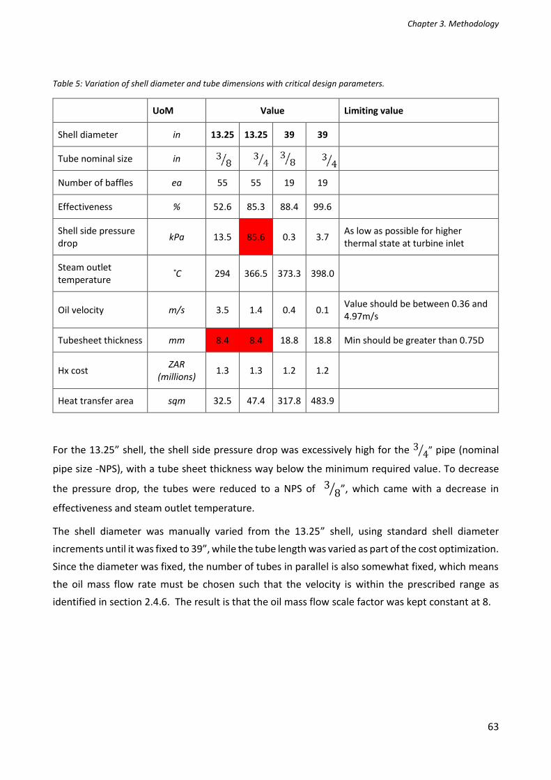
Chapter 3. Methodology
63
Table 5: Variation of shell diameter and tube dimensions with critical design parameters.
UoM Value Limiting value
Shell diameter in 13.25 13.25 39 39
Tube nominal size in
Number of baffles ea 55 55 19 19
Effectiveness % 52.6 85.3 88.4 99.6
Shell side pressure drop
kPa 13.5 85.6 0.3 3.7 As low as possible for higher thermal state at turbine inlet
Steam outlet temperature
˚C 294 366.5 373.3 398.0
Oil velocity m/s 3.5 1.4 0.4 0.1 Value should be between 0.36 and 4.97m/s
Tubesheet thickness mm 8.4 8.4 18.8 18.8 Min should be greater than 0.75D
Hx cost ZAR
(millions) 1.3 1.3 1.2 1.2
Heat transfer area sqm 32.5 47.4 317.8 483.9
For the 13.25” shell, the shell side pressure drop was excessively high for the 34⁄ ” pipe (nominal
pipe size -NPS), with a tube sheet thickness way below the minimum required value. To decrease
the pressure drop, the tubes were reduced to a NPS of 38⁄ ”, which came with a decrease in
effectiveness and steam outlet temperature.
The shell diameter was manually varied from the 13.25” shell, using standard shell diameter
increments until it was fixed to 39”, while the tube length was varied as part of the cost optimization.
Since the diameter was fixed, the number of tubes in parallel is also somewhat fixed, which means
the oil mass flow rate must be chosen such that the velocity is within the prescribed range as
identified in section 2.4.6. The result is that the oil mass flow scale factor was kept constant at 8.

Chapter 3. Methodology
64
Step 2: Shell and tube geometry selection
Tube size was selected as stainless steel (material recommended by HTF manufacturer) with a
nominal pipe size (NPS)5 of "
38
, schedule 40 and square pitch of 1.25”. TEMA standards were used
to select the tube hole diameters and standard tolerances.
25% segmental cut baffles were chosen, and with the fixed diameter, the actual baffle cut height,
baffle spacing, outer tube limit diameter and centre-line tube limit diameter were calculated.
Step 3: Tube sheet layout
Critical in HX design is ensuring that the calculated number of tubes fit inside the given shell
diameter. The number of tubes in the shell was calculated using equation (2.26) and the tube count
was then checked against the allowable count for that specific shell inside diameter [29, p. 841].
Step 4: Calculation of the shell leakage areas and correction factors for shell leakages
Equations from the Wolverine Tube, Inc Engineering Data Book III [32] were used to calculate the
baffle cut, baffle leakage, bundle by-pass and bundle spacing correction factors.
Step 5: Calculation of shell side heat transfer coefficient
An initial guess of the steam bulk fluid temperature and wall temperature was made. The ideal shell
side heat transfer coefficient was then calculated using equation (2.19), using the mean steam
temperature to calculate fluid properties and the actual heat transfer coefficient was calculated by
applying the adjustments as described in section 2.4.7.
Step 6: Calculation of tube side heat transfer coefficient
The oil flow rate was calculated by scaling the steam mass flow with the chosen scale factor. Using
the calculated oil flow rate, tube dimensions and oil viscosity, the Reynolds number was calculated,
including the effect of the tube count:
5 NB: Nominal Pipe size is not the actual pipe diameter, actual pipe dimensions were obtained from the ANSI 836.10 standard except in Table D-1 of the TEMA standard [21]

Chapter 3. Methodology
65
.
4
Re( 2 )
poil
toil
o tube oil
nm
n
D t
= −
The oil velocity was checked to confirm that it is within the suggested limits for the oil. The heat
transfer coefficient was then calculated using equation (2.21).
Step 7: Determination of overall heat transfer coefficient and HX outlet temperatures
The overall heat transfer coefficient was calculated, factoring in the corrected shell side heat
transfer coefficient and conduction wall resistance in the tube pipes. Using the calculated U value
and heat transfer area from tube count and geometry, the heater number transfer units were
calculated. The effectiveness was calculated using equation (2.17).
The pure counterflow heat exchanger assumption was employed as the calculated number of
baffles was greater than 10 for all the different scenarios under investigation. From the
effectiveness, the steam outlet temperature was calculated and checked to agree with the guessed
mean bulk shell fluid temperature. Using the energy balance equation, the oil outlet temperature
was also calculated, together with true temperature difference and the heat load of the heat
exchanger. The heat load will be used to calculate the size of the solar field, which is crucial in the
costing and performance evaluation section of the project. Lastly, the wall temperature was
calculated and compared to the initial guess.
Step 8: Determination of shell and tube side pressure drops
Tube-side pressure drops affect the pumping power required to pump the HTF. The tube-side
pressure drop was set to be at most 5% of the total turbine generated power. As outlined before in
section 2.4.7 above2.52.5 above, the detailed shell-side additional pressure drop calculations due
to the shell geometry are detailed in Appendix B of this report. The ideal shell diameter and tube-
geometry combination was the one with the lowest shell side pressure drop, in order to ensure the
highest possible thermal state at turbine inlet.
Step 9: Material cost
A tube sheet design was performed using the guidelines set out in Appendix A of the TEMA standard,
and the end heads were designed according to [47, pp. 815-823], using thick cylinder theory. Total
material cost was calculated as set out in Section 2.6 above. Material costs were obtained from Euro
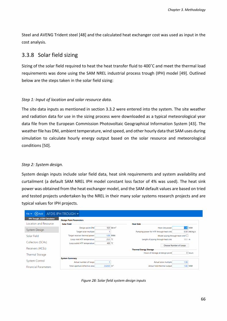
Chapter 3. Methodology
66
Steel and AVENG Trident steel [48] and the calculated heat exchanger cost was used as input in the
cost analysis.
3.3.8 Solar field sizing
Sizing of the solar field required to heat the heat transfer fluid to 400˚C and meet the thermal load
requirements was done using the SAM NREL industrial process trough (IPH) model [49]. Outlined
below are the steps taken in the solar field sizing:
Step 1: Input of location and solar resource data.
The site data inputs as mentioned in section 3.3.2 were entered into the system. The site weather
and radiation data for use in the sizing process were downloaded as a typical meteorological year
data file from the European Commission Photovoltaic Geographical Information System [43]. The
weather file has DNI, ambient temperature, wind speed, and other hourly data that SAM uses during
simulation to calculate hourly energy output based on the solar resource and meteorological
conditions [50].
Step 2: System design.
System design inputs include solar field data, heat sink requirements and system availability and
curtailment (a default SAM NREL IPH model constant loss factor of 4% was used). The heat sink
power was obtained from the heat exchanger model, and the SAM default values are based on tried
and tested projects undertaken by the NREL in their many solar systems research projects and are
typical values for IPH projects.
Figure 28: Solar field system design inputs

Chapter 3. Methodology
67
Step 3: Selection of the solar collector and receiver.
After design specifications, the next critical step was selection of the collector and the receiver. The
selected solar collectors were SkyFuel trough collectors as they are the most developed to date in
the parabolic trough systems, with efficiencies as high as 75% and the Schott PTR 80 receiver
because it is the largest on the market [7].
Step 4: Specification on the HTF and thermal storage requirements.
Since no thermal storage is required, only specifications for the heat transfer fluid, freeze protection
temperatures and flow rates were needed. The selected HTF was Therminol VP-1, using the HTF
specified operational limits as previously discussed.
Step 5: Results and running a parametric simulation for different heat loads.
For each different length of heat exchanger, a different heat load is calculated. A parametric
simulation was done for the different heat exchanger sizes by changing the Heat sink power input
in the model. This produced the required solar field size, capital costs, annual operational and fixed
maintenance costs and the annual thermal energy output.
3.3.9 Turbine Calculations
Based on the heat exchanger outlet steam temperature and required process plant thermal load
boundary conditions, the turbine work was calculated as follows:
Step 1: Determination of required turbine power to meet plant demand.
The SST-060 comes with a name-plate efficiency of 86% for the turbo-alternator and 95% for the
generator. Using those efficiency values, the turbine efficiency was calculated as 90.5%. Given that
the plant maximum demand is 621.68kW, the required generator input power was calculated as:
max..
demandgen in
generator
PP
=
Using the turbine efficiency, the required turbine power was calculated as:
.
.
gen in
turb required
turbine
PP
=
This is the required input power to the turbine if it were to fully meet the plant power demand.
Chapter 3. Methodology
68
Step 2: Calculation of turbine boundary conditions.
The turbine exhaust conditions are governed by the process steam plant requirements of 400kPa
and 100˚C and the heat exchanger steam outlet feeds into the turbine. Assuming a 5% pressure
drop in all the steam lines and governing valve, the turbine exhaust pressure was scaled up by 5%
to cater for steam line losses.
The turbine inlet pressure was calculated as the boiler pressure, minus the shell side pressure drop
and the 5% line and valve losses. The inlet enthalpy to the turbine is the heat exchanger steam exit
enthalpy.
Step 3: Calculation of actual turbine power.
The actual turbine exit enthalpy is calculated from the turbine efficiency equation, (2.30), and the
inlet and exit boundary conditions used to calculate the inlet enthalpy, ideal lossless turbine exit
enthalpy and turbine efficiency. From the actual exit enthalpy, the actual turbine power, steam
exit temperature and quality were calculated.
Step 4: Auxiliary power requirements and import power calculation.
Knowing the actual turbine power output, and the oil pump power requirement from the Heat
Exchanger Design analytical calculation, the auxiliary power requirement was checked to see if it
was in the 5% range of total power output (if too large, some changes to the shell diameter and oil
mass flow would be needed). The Sent-Out Power was then calculated as the difference between
the actual turbine output power and auxiliary oil pump power requirement, and power was
compared with the plant demand to calculate the imports required if any. The detailed turbine
calculation is attached in Appendix C of this report.
3.3.10 Project costing and optimization
The project capital costs were calculated as set out in section 2.8 and the heat exchanger length
varied to calculate the optimum heat exchanger size for this application. The heat exchanger length
determines the heat transfer area and by increasing or decreasing it, the actual work/heat load of
the heat exchanger is altered. This affects the thermal uptake of the system and subsequently the
solar field size requirement, which in turn increases or reduces the CAPEX of the project.
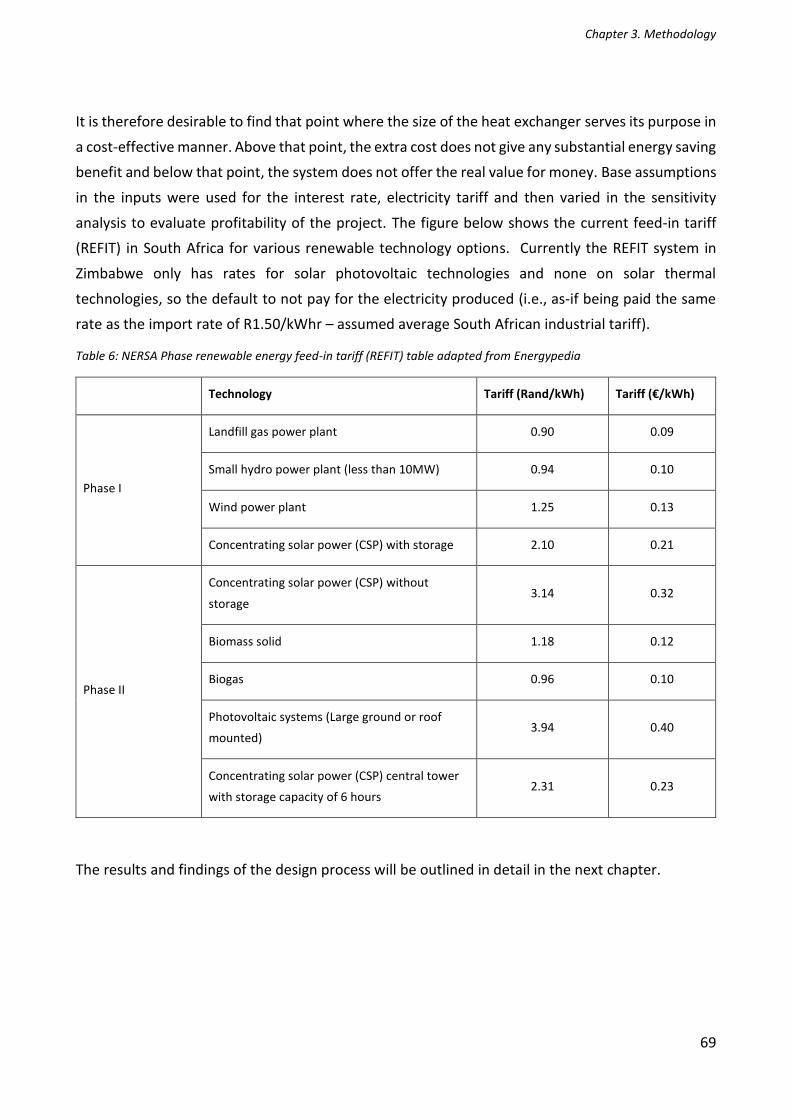
Chapter 3. Methodology
69
It is therefore desirable to find that point where the size of the heat exchanger serves its purpose in
a cost-effective manner. Above that point, the extra cost does not give any substantial energy saving
benefit and below that point, the system does not offer the real value for money. Base assumptions
in the inputs were used for the interest rate, electricity tariff and then varied in the sensitivity
analysis to evaluate profitability of the project. The figure below shows the current feed-in tariff
(REFIT) in South Africa for various renewable technology options. Currently the REFIT system in
Zimbabwe only has rates for solar photovoltaic technologies and none on solar thermal
technologies, so the default to not pay for the electricity produced (i.e., as-if being paid the same
rate as the import rate of R1.50/kWhr – assumed average South African industrial tariff).
Table 6: NERSA Phase renewable energy feed-in tariff (REFIT) table adapted from Energypedia
Technology Tariff (Rand/kWh) Tariff (€/kWh)
Phase I
Landfill gas power plant 0.90 0.09
Small hydro power plant (less than 10MW) 0.94 0.10
Wind power plant 1.25 0.13
Concentrating solar power (CSP) with storage 2.10 0.21
Phase II
Concentrating solar power (CSP) without
storage 3.14 0.32
Biomass solid 1.18 0.12
Biogas 0.96 0.10
Photovoltaic systems (Large ground or roof
mounted) 3.94 0.40
Concentrating solar power (CSP) central tower
with storage capacity of 6 hours 2.31 0.23
The results and findings of the design process will be outlined in detail in the next chapter.

Chapter 4. Results and Discussion
70
4. Results and Discussion
4.1 System Model
Figure 29: Proposed steam plant process flow diagram
The above P&ID diagram was developed to show the new steam and condensate flow if the steam
turbine topping cycle is retrofitted into the existing process steam plant. Steam leaves the boiler,
dry saturated at 950kPa, and is piped to the heat exchanger shell side, where it is superheated by
hot oil from the solar field, which flows in the tube side of the heat exchanger. The superheated
steam is expanded in the turbine, which exhausts at a pressure which is sufficient to ensure the
process steam thermal requirements are met. The generator is synchronized with the plant’s main
bus bar and feeds the generated electricity to the plant. There is a T-junction after the boiler, which
allows for by-passing the power block and feeding straight to the process steam plant in the case of
emergencies or low solar insolation when the power cycle is offline.
The following sections discuss the general system parameters and results from the analysis models
in Appendix B and C.
Chapter 4. Results and Discussion
71
4.2 Physical system parameters
Heat exchanger: Type BEM, Size 39 – 360 (991 – 9144) (base assumptions case)
Coal fired boiler output (steam inlet to the heat-exchanger)
• Mass flow: 2.5kg/s,
• Pressure: 950kPa,
• Temperature: 177.67 ˚C,
• Quality: dry saturated.
HTF to inlet conditions (hot fluid inlet into heat exchanger)
• HTF: Therminol VP-1,
• Mass flow: 20kg/s,
• Temperature: 400 ˚C.
Heat exchanger model outputs
• Shell diameter: 39” (990.6mm),
• Tubes length: 15 – 60ft. Based on the initial sizing, the first length chosen was 30 ft, and this
will be referred to as the Base case,
• Total heat transfer area: 158 – 637m2,
• Steam heat addition: 0.8 – 1.17MW,
• Heat exchanger effectiveness: 66.8 – 98.5%,
• Steam outlet temperature: 325.7 – 395.8 ˚C,
• Heat exchanger cost: mR0.64 – mR2.46.
Figure 30 below shows the steam heat addition requirement, versus the tube length.
6 mR0.64 means 0.64 million rands
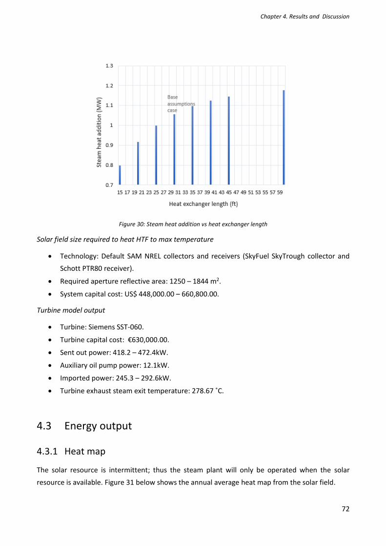
Chapter 4. Results and Discussion
72
Figure 30: Steam heat addition vs heat exchanger length
Solar field size required to heat HTF to max temperature
• Technology: Default SAM NREL collectors and receivers (SkyFuel SkyTrough collector and
Schott PTR80 receiver).
• Required aperture reflective area: 1250 – 1844 m2.
• System capital cost: US$ 448,000.00 – 660,800.00.
Turbine model output
• Turbine: Siemens SST-060.
• Turbine capital cost: €630,000.00.
• Sent out power: 418.2 – 472.4kW.
• Auxiliary oil pump power: 12.1kW.
• Imported power: 245.3 – 292.6kW.
• Turbine exhaust steam exit temperature: 278.67 ˚C.
4.3 Energy output
4.3.1 Heat map
The solar resource is intermittent; thus the steam plant will only be operated when the solar
resource is available. Figure 31 below shows the annual average heat map from the solar field.

Chapter 4. Results and Discussion
73
Figure 31: Timestep- averaged system outlet temperature
As expected, the solar collector performs better in the summer months, from mid-August to October
when the DNI is high. The system peaks to maximum outlet temperatures as early as 8am in the
morning and has very high outlet temperatures throughout the day in these months. From
November to May, the heat output oscillates between high and low in between days as this is usually
the rainy season in Zimbabwe, with the most rains falling around March which experiences the
lowest values of thermal energy output. This is because on rainy days, there is mostly cloudy
conditions reducing the incident beam radiation. From April to May the weather transitions to
winter, with winter falling between June and July. In winter there is also a lot of cloud cover which
will see some days not receiving beam radiation on thick cloud days.

Chapter 4. Results and Discussion
74
4.3.2 Daily hourly average thermal energy
Figure 32: Typical daily hourly average thermal energy variation per month for a 1.06 MW (base case) design heat sink power
Figure 32 above shows the daily hourly average incident thermal power on the collector (in blue),
and the outlet thermal energy delivered by the HTF to the heat sink from January to December (in
red) for the base case heat exchanger. One can see that the required 1.06MW of thermal energy is
essentially the maximum heat sink power the field can supply and occurs only in September. Since
the peak is achieved quite soon after sunrise, it is assumed that the required heat is available from
8:00 to 16:00 (8 hours) during the peak month. In subsequent solar field results, this will be termed
“Normal solar output”.
March, as shown in Figure 32 above, is the lowest output month with the system only delivering
slightly above half of the required thermal energy throughout the productive solar hours of the day.
To ensure that the heat exchanger heat load requirement is met throughout the year, the solar field
needs to be oversized. It was found that the solar field had to be scaled up by a factor of 1.65 to
ensure a theoretical constant maximum output during operation from 08:00 – 16:00 for the whole

Chapter 4. Results and Discussion
75
year (see Figure 33). This factor was then used to scale up the heat sink for different heat exchanger
lengths and the total investment, cash savings and subsequent payback period calculated. This will
be termed “Maximum solar output”.
The drawback with oversizing the solar field, is that excess energy during the peak months cannot
be used, and some portions of the collector must be shut to avoid overheating. It does however
enable maximum electricity production throughout the year, which may be financially more
beneficial compared to the extra capital investment.
Figure 33: Annual daily hourly average output required for solar output throughout the year.
4.3.3 Annual electricity production
For every 1.06MW input of thermal energy into the heat exchanger, the power cycle sends out
457.79kW of electrical power to the main busbar. The SAM model provided the net annual thermal
energy delivered to the heat sink, and using direct proportion, the annual energy production was
calculated. The table below shows the annual thermal energy output from the normal solar field
output, for all scenarios analysed, including maximum and minimum values.

Chapter 4. Results and Discussion
76
Table 7: Annual thermal and electrical energy output for a Normal solar field
Heat exchanger length (ft)
Q_heatsink_design (MWt)
Annual_energy_heat sink
(kWt-hr)
Max monthly output
(MWt-hr)
Min monthly output
(MWt-hr)
15 0.8 2.26E+06 243.93 172.95
20 0.9 2.48E+06 263.38 185.97
25 1.0 2.61E+06 280.97 194.32
30 1.06 2.71E+06 293.37 200.34
35 1.10 2.77E+06 301.53 204.22
40 1.13 2.81E+06 307.61 207.09
45 1.15 2.84E+06 311.68 209.03
60 1.18 2.88E+06 317.63 211.71
The net annual energy outputs for both the normal and maximum solar field outputs were obtained
by running a parametric simulation and using the heat sink power as input, and selecting the gross
and net annual thermal energy production as the output as shown in the figure below:
Figure 34: Annual thermal energy output for normal solar field

Chapter 4. Results and Discussion
77
The maximum and minimum monthly values were obtained from the Statistics tab in SAM [18]
Table 8: Annual thermal and electrical energy output for a Maximum solar field
Heat exchanger length (ft)
Q_heatsink_design (MWt)
Annual_energy_heat sink
(kWt-hr)
Max monthly output
(MWt-hr)
Min monthly output
(MWt-hr)
15 1.32 3.04E+06 344.11 223.18
20 1.51 3.17E+06 368.39 235.20
25 1.65 3.21E+06 372.42 236.77
30 1.75 4.80E+06 505.61 362.38
35 1.81 4.91E+06 519.97 368.89
40 1.86 4.99E+06 531.51 374.10
45 1.89 5.05E+06 538.34 377.29
60 1.94 5.14E+06 549.36 382.52
The maximum solar field heat sink power was calculated as explained in section 4.3.2, annual net
thermal energy obtained from the parametric simulation.

Chapter 4. Results and Discussion
78
4.4 System outputs
Table 9: System outputs
Item Description Units 1 2 3 4 5 6 7 8
in 39.0 39.0 39.0 39.0 39.0 39.0 39.0 39.0
ft 15.0 20.0 25.0 30.0 35.0 40.0 45.0 60.0
⁰C 325.7 347.6 362.8 374.2 381.0 386.2 390.0 395.8
MW 0.8 0.9 1.0 1.1 1.1 1.1 1.1 1.2
m 2 158.3 211.5 264.6 317.8 371.0 424.2 477.4 637.0
% 66.9 76.8 83.7 88.4 91.9 94.2 95.9 98.5
ZAR 640191.5 834786.0 1029380.5 1224192.8 1418569.6 1613164.1 1807758.6 2391542.2
m 2 1,250.0 1,438.0 1,563.0 1,656.0 1,719.0 1,766.0 1,797.0 1,844.0
USD 448,000.0 515,200.0 560,000.0 593,600.0 616,000.0 632,800.0 644,000.0 660,800.0
USD 6,400.0 7,360.0 8,000.0 8,480.0 8,800.0 9,040.0 9,200.0 9,440.0
m 2 2,063.0 2,359.0 2,578.0 2,719.0 2,828.0 2,906.0 2,953.0 3,031.0
USD 739,200.0 845,600.0 924,000.0 974,400.0 1,013,600.0 1,041,600.0 1,058,400.0 1,086,400.0
USD 10,560.0 12,080.0 13,200.0 13,920.0 14,480.0 14,880.0 15,120.0 15,520.0
Turbine SOP kW 418 435 447 458 461 465 468 472
kW 293 275 264 255 250 246 243 238
Euro 630,000 € 630,000 € 630,000 € 630,000 € 630,000 € 630,000 € 630,000 € 630,000 €
Heat transfer area
Shell & Tube Heat Exchanger, Type BEM
Shell inner
diameter
Tube length
Steam outlet
temperature
Heat input to steam
Turbine capital cost
Total required
aperture reflective
area
Effectiveness
Heat exchanger cost
External Solar Field Inputs
Normal solar field size
Capital costs
Operational costs
Total required
aperture reflective
area
Maximum solar output
Capital costs
Operational costs
Turbine Output
Import power
The created heat exchanger and turbine analysis models, together with the SAM solar simulation
package were used to analyse the system’s output, while varying the heat exchanger length. Heat
exchanger effectiveness, steam outlet temperature, turbine sent out and imported power and
equipment capital costs (shown in Table 9 above) were amongst the key output parameters. The
results were used for the financial analysis.

Chapter 4. Results and Discussion
79
4.5 Performance Evaluation
Figure 35: Variation of heat exchanger effectiveness and imported power with the heat exchanger length
As expected, the heat exchanger effectiveness increases with an increase in heat exchanger length.
This is because as the heat exchanger length increases, the greater the area available for heat
transfer and the closer the steam outlet temperature gets to the oil inlet temperature. However,
there are diminishing returns as the length increases, hence an excessively large heater would not
be financially viable. At 30ft length, the steam outlet temperature is 374.2˚C, and doubling the size
of the heat exchanger gives a steam outlet temperature of 396˚C, which is only 4.3˚C below the oil
inlet temperature. However, halving the length to 15 ft results in a steam outlet temperature of
325°C, which is 75°C below the achievable oil temperature.
From the project objectives, the designed system should meet the plant electrical maximum
demand of 621.68kW while still producing steam to the process at 400 kPa. This high exhaust
pressure means the steam is still superheated at the turbine outlet and will require de-superheating
spray to meet the 100°C temperature conditions. The downside of exhausting at such a high
backpressure is that the power cycle cannot meet the process plant electrical energy requirements,
and the deficit has to be imported from the grid supply. In all eight instances under investigation,
even at 98.5% heat exchanger effectiveness, the system did not produce enough electrical energy
to meet the process plant demand and the deficit must be imported from the grid. However, it was
noted that as the turbine output power increases the deficit reduces, decreasing the amount of

Chapter 4. Results and Discussion
80
power imported from the grid, as shown by the blue line in Figure 35. To get to the 621.68kW sent
out power from the generator, the following could be done:
• Increase mass flow,
• Increase the thermal state at turbine inlet,
• Reduce turbine exhaust pressure.
Option 1: Increase mass flow.
The power output is directly proportional to the steam mass flow. The mass flow of steam can be
increased by increasing the size of the boiler to 13.91tph, a 55% increase in the steam flow rate.
This implies purchasing a bigger size boiler which is not feasible as the additional steam which is not
used in the process must be condensed, increasing the system components, which escalates both
capital and operational costs. This also reduces the net thermal efficiency of the cycle as heat added
in the boiler and superheater section is lost in the condenser without doing any useful work.
Option 2: Increase thermal state at turbine inlet.
The thermal state at turbine inlet can be increased by either increasing the inlet pressure or inlet
temperature. Increasing the pressure is not an option as the boiler pressure cannot be altered
without changing the boiler itself. Increasing the temperature can be done by using a heat transfer
fluid which can be heated to more than the current HTF limit of 400˚C for Therminol VP-1. An option
will be using Hi-tec salt which can go as high up as 593˚C. Hi-Tec is not yet popular in practical CSP
applications due to its high freeze temperature of 235˚C. This freeze temperature is too high, for a
site like AFDIS with an average annual ambient temperature of 18.5˚C and no thermal storage. To
ensure the HTF flows through the system, a freeze protection system must be installed, which not
only increases the CAPEX and OPEX requirement, but poses a threat of operational challenges like
pipe blockages and need for more auxiliary power to keep the freeze protection system running.
Option 3: Reducing turbine exhaust pressure.
At 289kPa turbine exhaust pressure (28% reduction in exhaust pressure), using the base
assumptions, the sent-out power is 625.17kW. This reduction in turbine exhaust pressure increases
turbine output but goes against the original objective of providing power without altering the
original process thermal needs. To ensure that the process plant steam meets its boundary
conditions requirements (at 289kPa turbine exhaust pressure), it will thus be necessary to pressurize
the condensate to process steam pressure which is not technically feasible as the exhaust will still
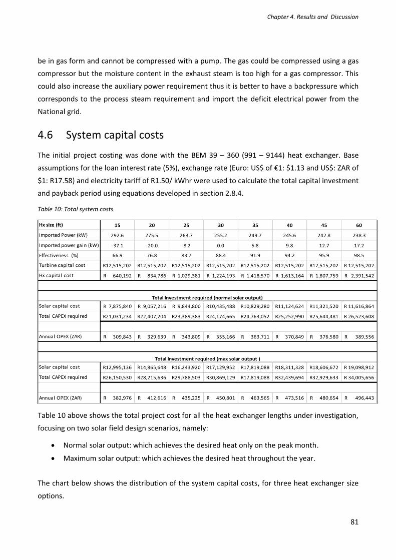
Chapter 4. Results and Discussion
81
be in gas form and cannot be compressed with a pump. The gas could be compressed using a gas
compressor but the moisture content in the exhaust steam is too high for a gas compressor. This
could also increase the auxiliary power requirement thus it is better to have a backpressure which
corresponds to the process steam requirement and import the deficit electrical power from the
National grid.
4.6 System capital costs
The initial project costing was done with the BEM 39 – 360 (991 – 9144) heat exchanger. Base
assumptions for the loan interest rate (5%), exchange rate (Euro: US$ of €1: $1.13 and US$: ZAR of
$1: R17.58) and electricity tariff of R1.50/ kWhr were used to calculate the total capital investment
and payback period using equations developed in section 2.8.4.
Table 10: Total system costs
15 20 25 30 35 40 45 60
292.6 275.5 263.7 255.2 249.7 245.6 242.8 238.3
-37.1 -20.0 -8.2 0.0 5.8 9.8 12.7 17.2
66.9 76.8 83.7 88.4 91.9 94.2 95.9 98.5
12,515,202R 12,515,202R 12,515,202R 12,515,202R 12,515,202R 12,515,202R 12,515,202R 12,515,202R
640,192R 834,786R 1,029,381R 1,224,193R 1,418,570R 1,613,164R 1,807,759R 2,391,542R
7,875,840R 9,057,216R 9,844,800R 10,435,488R 10,829,280R 11,124,624R 11,321,520R 11,616,864R
21,031,234R 22,407,204R 23,389,383R 24,174,665R 24,763,052R 25,252,990R 25,644,481R 26,523,608R
309,843R 329,639R 343,809R 355,166R 363,711R 370,849R 376,580R 389,556R
12,995,136R 14,865,648R 16,243,920R 17,129,952R 17,819,088R 18,311,328R 18,606,672R 19,098,912R
26,150,530R 28,215,636R 29,788,503R 30,869,129R 17,819,088R 32,439,694R 32,929,633R 34,005,656R
382,976R 412,616R 435,225R 450,801R 463,565R 473,516R 480,654R 496,443R
Hx size (ft)
Imported Power (kW)
Imported power gain (kW)
Effectiveness (%)
Turbine capital cost
Hx capital cost
Total Investment required (normal solar output)
Total Investment required (max solar output )
Solar capital cost
Annual OPEX (ZAR)
Solar capital cost
Total CAPEX required
Annual OPEX (ZAR)
Total CAPEX required
Table 10 above shows the total project cost for all the heat exchanger lengths under investigation,
focusing on two solar field design scenarios, namely:
• Normal solar output: which achieves the desired heat only on the peak month.
• Maximum solar output: which achieves the desired heat throughout the year.
The chart below shows the distribution of the system capital costs, for three heat exchanger size
options.

Chapter 4. Results and Discussion
82
Figure 36: System capital costs breakdown
Figure 36 above shows the capital cost breakdown for the 15ft, 30ft and 60ft heat exchanger. The
turbo-alternator capital costs contribution to the CAPEX decreased with increase in HX length
although it was the most capital-intensive item in all the systems. Solar thermal field capital costs
were the next capital-intensive variable, increasing with increase in HX length. Although the heat
exchanger costs appear insignificant compared to the other two cost drivers, it is important to note
that there is direct proportionality between heat exchanger size and solar field capital costs as the
amount of thermal heat input determines the solar field size. Despite using the same turbo-
alternator in all three instances, the smaller HX lengths had the lowest heat transfer area, which
translated to the lowest HX capital costs. This in turn made the contribution of the turbo-alternator
costs to the CAPEX decrease with increase in HX costs.

Chapter 4. Results and Discussion
83
4.7 Payback period and optimal length
4.7.1 Normal solar output
Figure 37: Total investment required and payback period vs heat exchanger length for normal solar output
It is evident that there appears to be an optimum point (about 30 ft) where the payback period is a
minimum for a given heat exchanger length. For smaller lengths, the cash savings due to electricity
production are too low compared to the CAPEX requirement. Larger heat exchanger lengths do not
give enough cash saving benefit to outweigh the CAPEX increase. The payback period is in the range
of 40 -50 years for all scenarios under investigation. This is not economically viable as the technical
lifespan of most solar thermal plants is at most 25 years.
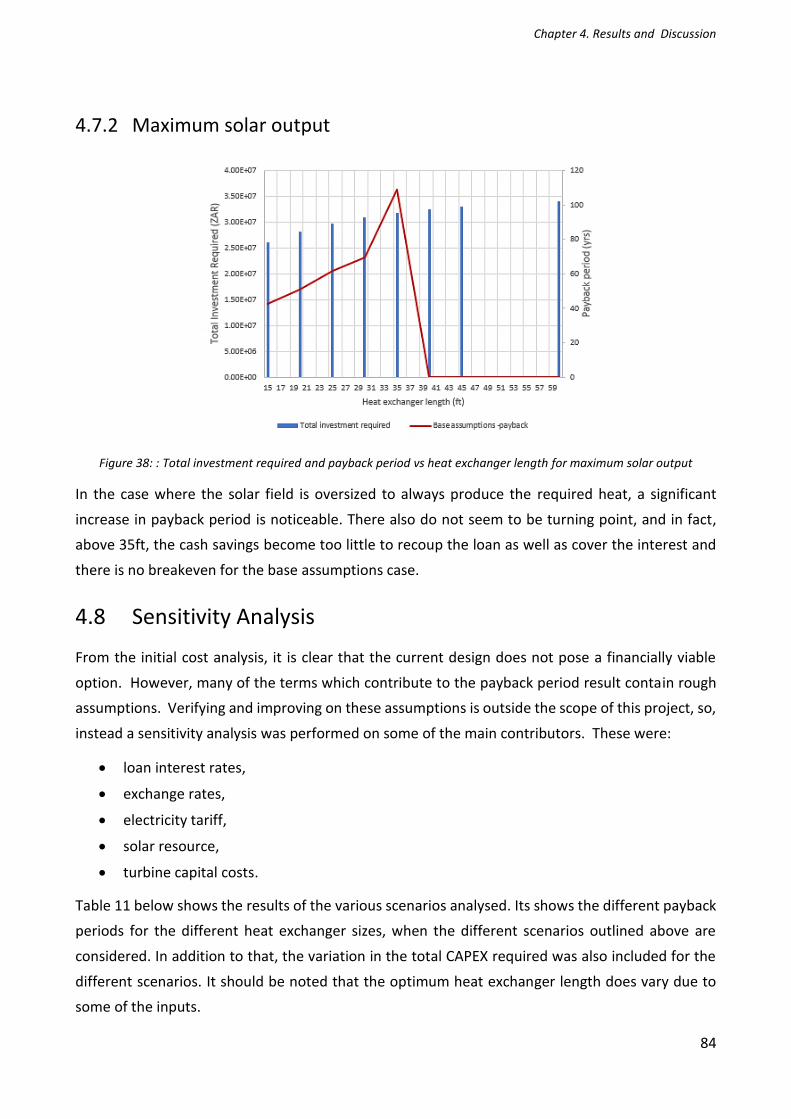
Chapter 4. Results and Discussion
84
4.7.2 Maximum solar output
Figure 38: : Total investment required and payback period vs heat exchanger length for maximum solar output
In the case where the solar field is oversized to always produce the required heat, a significant
increase in payback period is noticeable. There also do not seem to be turning point, and in fact,
above 35ft, the cash savings become too little to recoup the loan as well as cover the interest and
there is no breakeven for the base assumptions case.
4.8 Sensitivity Analysis
From the initial cost analysis, it is clear that the current design does not pose a financially viable
option. However, many of the terms which contribute to the payback period result contain rough
assumptions. Verifying and improving on these assumptions is outside the scope of this project, so,
instead a sensitivity analysis was performed on some of the main contributors. These were:
• loan interest rates,
• exchange rates,
• electricity tariff,
• solar resource,
• turbine capital costs.
Table 11 below shows the results of the various scenarios analysed. Its shows the different payback
periods for the different heat exchanger sizes, when the different scenarios outlined above are
considered. In addition to that, the variation in the total CAPEX required was also included for the
different scenarios. It should be noted that the optimum heat exchanger length does vary due to
some of the inputs.

Chapter 4. Results and Discussion
85
Color based formatting was used to highlight and differentiate the payback periods for the different
heat exchnager lengths, with the green colour scheme showing the lowest payback and thus
optimum heater length for each scenario and red showing the largest payback period. Where the
cell returns the #NUM! value, it means the cash saving is too low to recoup the capital investment7.
7 From equation (2.37), when the cash savings are too little, the term in the brackets becomes negative as the quotient becomes greater than one, thus the formula returns the #NUM! error as there is no natural logarithm for negative numbers.

Chapter 4. Results and Discussion
86
Table 11: Sensitivity Analysis Results
15 20 25 30 35 40 45 60
48.68 42.86 40.81 40.48 40.74 41.54 42.45 46.23
48.68 42.86 40.81 40.48 40.74 41.54 42.45 46.23
9.65 9.30 9.15 9.12 9.14 9.20 9.27 9.51
17.1 18.3 19.1 19.8 20.3 20.7 21.1 21.9
24.61 23.25 22.74 22.72 22.87 23.20 23.55 24.85
7.28 7.05 6.96 6.96 6.99 7.05 7.11 7.32
14.8 15.8 16.5 17.1 17.5 17.9 18.3 19.0
18.10 17.25 16.94 16.94 17.06 17.28 17.53 18.44
6.04 5.85 5.78 5.78 5.81 5.86 5.92 6.12
#NUM! #NUM! #NUM! #NUM! #NUM! #NUM! #NUM! #NUM!
24.37 23.29 22.84 22.77 22.83 23.01 23.21 23.95
8.46 8.19 8.08 8.06 8.07 8.12 8.17 8.36
1260.88 1361.46 1452.35 1516.44 1558.62 1590.04 1611.12 1641.85
21.91 21.28 20.33 19.91 19.77 19.76 19.85 20.46
893.98 961.31 1004.47 1035.59 1055.63 1070.48 1080.50 1094.34
#NUM! #NUM! #NUM! #NUM! #NUM! #NUM! #NUM! #NUM!
19.2 20.5 21.5 22.3 22.9 23.4 23.8 24.6
33.36 31.35 30.65 30.73 31.05 31.63 32.24 34.48
17.9 19.3 20.3 21.0 21.6 22.1 22.5 23.4
27.46 26.38 26.08 26.28 26.62 27.13 27.65 29.43
Heat Exchanger size (ft)
Base assumptions case
(interest rate 5%, tariff
Variation of Feed- in- Tariff
Sell at the price you buy at
from ESKOM)
With NERSA Tariff
Turbine CAPEX less by 15%
Variation of USD/ ZAR & Euro/USD exchange rate
Total investment required
(ZAR mill ion)Sell at the price you buy at
from ESKOM)
With NERSA Tariff
5 year average (US$1: R14.21; US$1: 1.13€ )
With NERSA Tariff and
2.5% interest rate
10 year average (US$1: R11.66; US$1: 1.217€)
Design for highest insolation month (September)
Design for lowest insolation month (March)
Payback period (years)
Variation of solar resource
Annual electrical energy
produced (MWhrpeak)
Payback period (years)
Annual electrical energy
produced (MWhrpeak)
Payback period (years)
Interest at 2.5%
Turbine CAPEX less by 25%
Total investment required
(ZAR mill ion)
Payback period (years)
Total investment required
(ZAR mill ion)
Total investment required
(ZAR mill ion)
Sell at the price you buy at
from ESKOM)
With NERSA Tariff
Variation of Interest rate
Interest at 7%
Variation of turbine capital costs

Chapter 4. Results and Discussion
87
Electricity tariff
The electricity tariff proved to be the deciding factor on the profitability of this project. Using the
REFIT tariff, the payback period dropped from the range of 40 – 50 years in the base assumptions
case to about 9 - 10 years, which is reasonable for such an investment. The payback period is even
reduced further if the REFIT tariff is coupled with an interest rate lower than 5%.
Variation of the exchange rates (Euro/US$ and US$/ZAR)
The turbine capital cost was quoted in Euros and the solar field sizing was done using a software
giving costs in US$. The effect of the exchange rate on the payback period was also analysed, given
that the financial analysis was performed based on the South African rand. The five- and ten-year
averages for the currencies were used to check the effect on the payback period. It was shown that
for the 5-year averages, the project is not economically feasible, but using the ten-year average,
payback period is below 20 years.
However, using the REFIT scheme, the payback period for both the five- and ten-year average
exchange rates falls to a promising 6.96 and 5.78 years respectively. This shows that the project
might be economically feasible in the future if the rand gains strength to the dollar and euro and
the equipment capital costs decrease due to better technological advancement and competition in
both the turbine manufacturing and CSP industries, similar to what happened to the solar
photovoltaic energy capital costs in the past decade.
Loan interest rate
At high interest rates, greater than 5%, the project is not commercially viable as the cash savings
are too low to recoup the initial investment. At an interest rate of 2.5%, the payback period almost
halves to between 20 and 25 years, which is still not acceptable as it means the loan repayment will
run through the course of the plant’s technical lifespan.
Design for a worst- and best-case solar resource day
The best and worst resource months for the location were September and March. Options were
analysed as-if the system will receive these outputs all year round for the Normal solar output case.
It can be seen that for the best solar resource case, the payback period is almost half that of the

Chapter 4. Results and Discussion
88
base assumptions case, but still too high considering the plant technical lifespan. For the worst solar
resource scenario, the project is not economically viable.
Turbine capital costs
Turbine capital costs account for 52% of the system total CAPEX, based on a non-binding quote from
2016 of the Siemens SST-060 TG set. This quote may be inaccurate and does not include potential
cost negotiations. However, even by reducing the turbine costs by 15% and 25%, the payback period
was still longer than the technical lifespan of the plant.
The figure shows a summary of cases where the minimum payback period is less than 40 years,
along with the optimum heat exchanger length. From the figure, it is safe to conclude that the
optimum heat exchanger length is generally 30ft. There are a few cases with a payback period less
than 20 years, though these might be considered hypothetical. Most of the scenarios result in
excessive paybacks, making the project economically unfeasible.

Chapter 5. Conclusions and Recommendations
89
5. Conclusions and Recommendations
5.1 Conclusion
Chapter 1 gave a brief background to the research problem and objectives of the study. Literature
pertinent to the study was discussed in Chapter 2, placing emphasis on what is already there and
how the researcher would develop the system from existing models. In Chapter 3, the model was
developed, beginning with analysis of the qualitative data obtained from site visits and merging it
with the quantitative data gathered in the literature review. The results from the created models in
Chapter 3 (including the performance evaluation and economic analysis) were discussed in Chapter
4, focusing on the base assumptions case.
From the above findings, it was concluded that although it is technically possible to convert an
existing process steam plant into a combined heat and power plant using an external solar field
without affecting the process thermal load requirements, the project is not yet economically viable
on an independent investor financing model as it was established that the payback period is largely
dependent on the tariff.
Although the NERSA REFIT for CSP projects without storage is R3.14/kWhr, which gives a positive
reasonable payback period of 9.12 years for the optimum heat exchanger length, the tariff which is
considered is the tariff the process plant buys its electricity from the power supply Authority not the
feed in tariff. Unless the government offers an incentive of topping up the deficit of the REFIT to the
process plant’s savings to encourage the uptake of CSP projects, the project remains economically
unviable until the CAPEX requirement for the solar and turbine technologies decreases.
However, it is also important to note that the need for this research came from the fact that most
industries were losing uptime due to the rampant load shedding, affecting their revenue streams.
Another downside of load-shedding is shorter equipment lifespans (particularly on electric motors
which get damaged on start-ups and overload failures on shaft couplings and gearboxes on the
drivetrains). During drive-train design of process plant equipment, the gearbox is sized for
continuous operation and daily start-stops during load-shedding increase the possibilities of
overload failure due to cyclic loading. By using the solar assisted power cycle to kick in just before
power is switched off, the companies can keep their plants running during load-shedding and
maintain their production volumes. This avoids revenue losses due to load-shedding, which if
converted into monetary value can also add to the annual cash flows and decrease the payback
period significantly.

Chapter 5. Conclusions and Recommendations
90
The downside of switching the power cycle on and off however is the introduction of thermal cycles
in the system, which deteriorates the heat exchanger and piping system material. With that said,
tube leaks in the heat exchanger will be expected in 5 years, and piping bends should be replaced
within 10 years.
5.2 Recommendations
Recommendations for further research
• Given a chosen heat exchanger size, it would be beneficial to develop a comprehensive
process model that links the solar field actual heat uptake with the power block, thereby
enabling more accurate annual savings calculations.
• A more detailed cost model can be employed particularly in the heat exchanger
manufacturing costs using the generic model developed by Caputo et al [42], as well as other
system costs that may have been overlooked.
• Solar system optimization by exploring the benefit of employing thermal storage, particularly
in this era when there is more research on the use of molten salts as HTFs which can attain
temperatures as high as +500˚C.
• A thorough cost benefit analysis should be done considering the monetary value of
intangible benefits like maintaining the plant availability in the event of load shedding.
• Use of other profitability indicators like Net Present Value and Internal Rate of Return to
check the economic viability of the project.
Recommendations for process steam plants
The energy sector is already experiencing massive shifts to renewable energy sources in a bid to
curb the effects of climate change caused by greenhouse gas emissions. It would be a noble
development to do a thorough feasibility assessment to evaluate profitability of such a project.
The benefits of cogeneration cannot be overemphasized again in this section as it is evident that
cogeneration not only reduces the carbon footprint of a coal fired process steam plant, but also
offers a reliable power source. In this era where most African power utilities are struggling to meet
rise in demand and opting for load-shedding during peak demand, cogeneration will go a long way
in minimizing revenue losses being experienced by most companies during load shedding.

Chapter 5. Conclusions and Recommendations
91
Recommendations for energy regulatory bodies
It is time more lucrative incentives are put in place to ensure that independent investors can invest
in the supply of renewable energies in Africa. European and Asian energy policies are already shifting
to renewables due to the adverse effects on the climate of brown power generation. China, the
largest producer of electricity in the world and also the largest emitter is already taking strides to
phase out less efficient systems in its High Efficiency Low Emissions (HELE) blueprint [51], and if
Africa adopts energy efficiency centred policies to merge the renewables and brown technologies,
it can both reduce its energy poverty and boost productivity.
The government should provide additional incentives, other than renewable energy feed-in tariffs
like equity or debt based financial instruments to encourage the uptake of solar thermal projects at
private investor levels. One way of offering such incentives is topping up the cost savings for the
process plant, by adding the deficit ESKOM will not pay to the investor (difference between NERSA
REFIT and the price the process plant buys the electricity from ESKOM) either in cash or as an
investment tax credit.
Retrofitment of process steam plants to enable cogeneration, after a thorough financial feasibility
study is a noble idea. However, the question to go to SAPG or just traditional steam cogeneration
plants still relies on the competitiveness of solar thermal technology, whose costs have remained
quite high compared to solar photovoltaic systems in the past decade. Most SAPG projects have
failed to take off due to high technology costs.

Bibliography
92
6. Bibliography
[1] C. Trimble, M. Kojima, I. P. Arroyo and M. Farah, “Financial Viability of Electricity Sectors in Sub-Saharan Africa: Quasi-Fiscal Deficits and Hiddne Costs,” World Bank Group: Energy and Extractives Global Practice Group, 2016.
[2] T. D. Eastop and A. McConkey, Applied Thermodynamics for Engineering Technologists, Delhi: Dorling Kindersley (India) Pvt. Ltd, 2009.
[3] Y. M. A. B and C. A, Thermodyanmics: An Engineering Approach, 5th Edition, Boston: McGraw-Hill College, 2006.
[4] J. Veerapa and M. Beerepoot, “Cogeneration and Renewables: Solutions for a low carbon energy future,” International Energy Agency, Paris, 2011.
[5] B. F. Kolanowski, Small Scale Cogeneration Handbook Second Edition, Georgia: The Fairmont Press, Inc, 2003.
[6] J. A. Duffie and W. A. Beckman, Solar Engineering of Thermal Processes, Fourth Edition, John Wiley & Sons, Inc, 2013.
[7] National Renewable Energy Laboratory, “SkyFuel Parabolic Trough Optical Efficiency Testing: Cooperative Research and Development Final Report,” U.S. Department of Energy, Oak Ridge, 2010.
[8] W. T. Pierce, “Solar Assisted Power Generation (SAPG): Investigation of Solar Preheating of Feedwater,” Stellenbosch University http://scholar.sun.ac.za, Stellenbosch, 2013.
[9] M. Petrov, M. Popa and T. Fransson, “Solar Augmentation of conventional steam plants: From system studies to reality,” in Proceedings of WREF 2012, Denver, 2012.
[10] Y. Yang, Q. Yan, R. Zhai, A. Kouzani and E. Hu, “An efficient way to use medium or low temperature solar heat for power generation - integration into conventional power plant,” Applied Thermal Engineering, no. 31, pp. 157-162, 2011.
[11] E. Hu, Y. Yang, A. Nishimura, F. Yilmaz and A. Kouzani, “Solar Thermal Aided Power Generation,” Applied Energy, no. 87, pp. 2881-2885, 2010.
[12] J. Gottshe and T. Hove, “Mapping global, diffuse and beam solar radiation in Zimbabwe,” Renewable Energy an International Journal, pp. 3-7, 1998.
[13] M. P. Petrov, M. Salomon Popa and T. H. Fransson, “Solar Augmentation of conventional steam plants,” in World Renewable Energy Forum, WREF 2012, Colorado, 2012.
[14] S. Mills, “Combining solar power with coal fired power plants, or co-firing natural gas,” Clean Energy, vol. 2, no. 1, pp. 1-9, 2018.
[15] Google Inc, “Google Images,” [Online]. Available: https://www.google.com/search?safe=active&tbs=simg:CAESlwIJmhwclhKV_1k8aiwILELCMpwgaYQpfCAMSJ9IUnQuBFtMU5wLWFUumA5Ie0xXuOKoqlyuEP7oq0TjNOPcijDmwKhowbdu3wvZdpKmBmQ_1xNu9qaMK3OO7w8h6--iPlhaPcp0sY0mGwxJTcQSTeIC2Otg1sIAQMCxCOrv4IGgoKCAgBEgS63XJODAsQne3BCRqEAQ. [Accessed 4 October 2020].

Bibliography
93
[16] AUSTELA, “Australian Solar Thermal Energy Association,” 2020. [Online]. Available: http://www.austela.net.au/newsletter/122-solar-boost-at-liddell-hunter-valley. [Accessed 2020].
[17] CS Energy, “Solar Boost Project: End of project report on the Kogan Creek Power Station,” ARENA, Queensland, 2016.
[18] Alliance for Sustainable Energy, LLC, System Advisor Model Help.
[19] G. F. Hewitt and S. J. Pugh, “Approximate Design and Costing Methods for Heat Exchangers,” Heat Transfer Engineering, vol. 28, no. 2, pp. 76-86, 2007.
[20] Alfa Laval, “Alfa Laval - Plate Technology,” 2020. [Online]. Available: https://www.alfalaval.com/globalassets/documents/industries/chemicals/petrochemicals/brochure_alfa_laval_plate_technology_ppm00063en.pdf. [Accessed February 2020].
[21] Tubular Exchanger Manufacturers Association, Standards of the Tubular Exchanger Manufacturers Association, Ninth Edition, New York: Tubular Exchanger Manufacturers Association, Inc, 2007.
[22] J. E. Edwards, “Design and Rating Shell and Tube Heat Exchangers,” MNL 032A, pp. 1-30, 29 August 2008.
[23] T. Kuppan, Heat Exchanger Design Handbook, New York: Marcel Dekker, Inc, 2000.
[24] F. P. Incropera, D. P. Dewitt, T. L. Bergman and A. S. Lavine, Fundamentals of Heat and Mass Transfer, Sixth Edition, New Jersey: John Wiley & Sons, Inc, 2007.
[25] A. N. Caglayan and P. Buthod, “Factors to correct air cooler and shell and tube exchanger LMTD,” Oil and Gas Journal, vol. 6, pp. 91-94, 1976.
[26] J. Ball, “Construction Basics of Shell and Tube Heat Exchangers,” API Heat Transfer, 1 March 2000.
[27] Enerquip Administrator, “Enerquip: The Helpful Heat Exchanger Experts,” 26 March 2018. [Online]. Available: https://www.enerquip.com/2018/03/26/7-shell-configurations-what-you-need-to-know-when-designing-a-shell-and-tube-heat-exchanger/. [Accessed 16 February 2020].
[28] Enerquip administrator, “Enerquip: The Helping Heat Exchanger Experts,” 26 March 2018. [Online]. Available: https://www.enerquip.com/2018/03/26/tubeside-or-shellside-comparing-fluid-allocation-options-for-your-shell-and-tube-heat-exchanger/. [Accessed 16 February 2020].
[29] D. Q. Kern, Process Heat Transfer, Tokyo: Mc-Graw Hill Book Company, Inc, 1965.
[30] Chemstations, Inc, CHEMCAD THERM Version 5.1 User Guide.
[31] Eastman Therminol, “Therminol - Heat Transfer Fluids by Therminol,” 2019. [Online]. Available: https://info.therminol.com/WF_2019_HTF_Calculator_Download-2.html#_ga=2.139334070.44303310.1592303265-1194112209.1592303265. [Accessed 31 October 2019].
[32] Wolverine Tube, Inc, “Single-Phase Shell-Side Flows and Heat Transfer,” in Engineering Data Book III, pp. 3-1 - 3-20.
[33] P. Subbarao, “Indian Institute of Technology, Delhi,” 14 February 2006. [Online]. Available: http://web.iitd.ac.in/~pmvs/courses/mel709/SHTE.pdf. [Accessed 23 March 2020].
Bibliography
94
[34] F. C. Magazoni, L. Cabezas-Gomez, P. F. Alvarino and J. M. Saiz-Jabardo, “Thermal Performance of One-Pass Shell and Tube Heat Exchangers in Counter-Flow,” Brazilian Journal of Chemical Engineering, vol. 36, no. 02, pp. 869-883, 2019.
[35] T. N. Raval and R. Patel, “Optimization of Auxiliary Power Consumption of Combined Cycle Power Plant,” Procedia Engineering, pp. 751-757, December 2013.
[36] S. Teir, Steam Boiler Technology, Second Edition, Helsinki: Helsinki University of Technology Department of Mechanical Engineering, Enenrgy Engineering and Environmental Protection Publications, 2003.
[37] E. F. Church, Steam Turbines, First Edition, New York: McGraw-Hill Book Company Inc, 1928.
[38] Howden Group, “Howden Group Products,” [Online]. Available: https://www.howden.com/en-gb/products/steam-turbines. [Accessed 23 March 2020].
[39] Siemens Turbomachinery Equipment (STE) GmbH, “IEA BioEnergy Task 32/33: Workshop on State-of-the-art technologies for small biomass co-generation, Copenhagen, Oct 7, 2010,” in Steam turbines: What is the lower limits for feasibility, recent developments to reduce costs and increase efficiency on small steam turbine systems, Reiner Schenk, Siemens Frankenthal, Germany, Copenhagen, 2010.
[40] P. Konstantin and M. Konstantin, Power and Energy Systems Engineering Economics: Best Practice Manual, Burgstetten: Springer International Publishing, AG, 2017.
[41] H. B. Foumani, “Manufacturing Cost Optimization of A Shell & Tube Heat Exchanger using the Differential Evolution Algorithm,” Lappeenranta University of Technology, Lappeenranta, Finland, 2018.
[42] A. Caputo, P. M. Pelagagge and P. Salini, “Manufacturing cost model for heat exchangers optimization,” Applied Thermal Engineering, no. 94, pp. 513 - 533, 2016.
[43] “European Commision Photovoltaic Geographical Information System,” [Online]. Available: https://re.jrc.ec.europa.eu/pvg_tools/en/tools.html#TMY.
[44] “sam.nrel.gov”.
[45] Coastal Chemical Co, L.L.C., “HITEC Heat Transfer Salt,” Brenntag Company, Texas.
[46] The International Association for the Properties of Water and Steam, “Revised Release on the IAPWS Industrial Formulation 1997 for the Thermodynamic Properties of Water and Steam,” The International Association for the Properties of Water and Steam, Lucerne, 2007.
[47] R. K. Sinnott, Coulson & Richardsons Chemical Engineering: Chemical Engineering Design, Volume 6, Fourth Edition, Oxford: Elsevier Butterworth-Heinemann, 2005.
[48] Aveng Trident Steel, “Aveng Trident Steel Product Catalogue,” 2020. [Online]. Available: http://www.aveng.co.za. [Accessed 10 March 2020].
[49] National Renewable Energy Laboratory, System Advisor Model Industrial Process Heat, 2020.
[50] P. Gilman, “Using parabolic trough field collector DNI for tower (salt),” 08 February 2017. [Online]. Available: sam.nrel.gov/forum/forum-general/1658-using-parabolic-trough-field-collector-dni-for-tower-salt.html. [Accessed 2020].
[51] I. C. C. Centre, Composer, China - Policies, HELE technologies and CO2 reductions. [Sound Recording]. International Energy Agency Clean coal centre. 2016.

Bibliography
95
[52] J. P. Laudon and K. C. Laudon, Essentials of Management Information Systems, New Jersey: Prentice Hall international editions, 2003.
[53] J. A. Duffie and W. A. Beckman, Solar Engineering of Thermal Processes, New Jersey: John Wiley & Sons,Inc, 2013.
[54] “Energypedia,” [Online]. Available: https://energypedia.info/wiki/South_African_Renewable_Energy_Feed-in_Tariff. [Accessed 19 August 2020].
[55] Verein Deutscher Ingenieure, VDI- Gesellschaft Verfahrenstechnik und Chemieingenieurwesen GVC, VDI Heat Atlas, Second Edition, Dusseldorf: Springer, 2010.
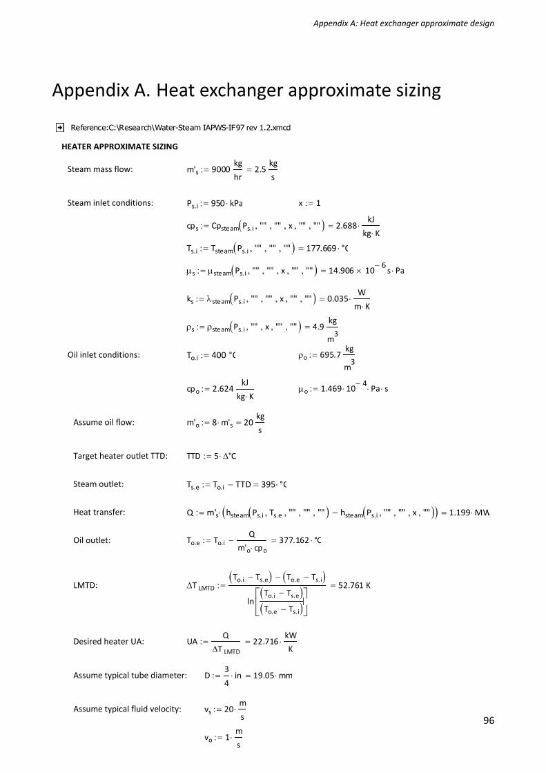
Appendix A: Heat exchanger approximate design
96
Appendix A. Heat exchanger approximate sizing
HEATER APPROXIMATE SIZING
Steam mass flow:
Steam inlet conditions:
Oil inlet conditions:
Assume oil flow:
Target heater outlet TTD:
Steam outlet:
Heat transfer:
Oil outlet:
LMTD:
Desired heater UA:
Assume typical tube diameter:
Assume typical fluid velocity:
Reference:C:\Research\Water-Steam IAPWS-IF97 rev 1.2.xmcd
m's 9000kg
hr2.5
kg
s==
Ps.i 950 kPa= x 1=
cps Cpsteam Ps.i "" "" x "" "" ( ) 2.688kJ
kg K==
Ts.i Tsteam Ps.i "" "" "" ( ) 177.669 °C==
s steam Ps.i "" "" x "" "" ( ) 14.906 106−
s Pa==
ks steam Ps.i "" "" x "" "" ( ) 0.035W
m K==
s steam Ps.i "" x "" "" ( ) 4.9kg
m3
==
To.i 400 °C= o 695.7kg
m3
=
cpo 2.624kJ
kg K= o 1.469 10
4− Pa s=
m'o 8 m's 20kg
s==
TTD 5 °C=
Ts.e To.i TTD− 395 °C==
Q m's hsteam Ps.i Ts.e "" "" "" ( ) hsteam Ps.i "" "" x "" ( )−( ) 1.199 MW==
To.e To.iQ
m'o cpo− 377.162 °C==
T LMTD
To.i Ts.e−( ) To.e Ts.i−( )−
lnTo.i Ts.e−( )To.e Ts.i−( )
52.761 K==
UAQ
T LMTD
22.716kW
K==
D3
4in 19.05 mm==
vs 20m
s=
vo 1m
s=

Appendix A: Heat exchanger approximate design
97
Steam side heat transfer:
Oil side heat transfer:
Overall heat transfer:
Required heater area:
Number of tubes in parallel:
Total length of a single tube:
Shell outer diameter:
Clearance: 300mm< DS < 1000mm, clearance = 0.5in
Outer tube limit diameter:
Shell diameter:
Prs
cps s
ks
1.144== Res
s vs D
s
125240.512==
Nus 0.36 Res0.55
Prs0.33
239.529==
hs
Nus ks
D440.311
W
m2
K
==
Pro
cpo o
ko
5.083== Reo
o vo D
o
90218.414==
Nuo 0.027 Res0.8
Prs0.33
337.952==
ho
Nuo ko
D1345.421
W
m2
K
==
U1
hs
1
ho
+
1−
331.743W
m2
K
==
AHTUA
U68.405 m
2==
nt
m'o
o vo1
4 D
2
100.862==
Lt
AHT
nt D37.179 ft==
Ltp 1.25 D= CL 1= CTP 0.90=
Dctl
4 nt CL Ltp2
CTP11.199 in==
Lbb 12.7mm=
Dotl Dctl D+ 0.303 m==
DS Dotl Lbb+ 12.449 in==

Appendix B. Heat exchanger program code
98
Appendix B. Heat exchanger program code
1. SYSTEM INPUTS
1.1 Problem specification: Heat exchanger inlet and exit conditions for steam
NB: Boiler exit & turbine inlet are heat exchanger inlet & exit respectively, assuming constant mass flow
Boiler exit:
Turbine inlet:
1.2 Fluid properties and flow arrangements
Shell side: Steam
Mass flow:
Inlet conditions:
Tube side: Therminol VP 1 oil from external solar source
Inlet conditions:
Fluid properties sourced from Therminol Fluid Properties calculator: https://info.therminol.com/WF_2019_HTF_Calculator_Download-2.html#_ga=2.139334070.44303310.1592303265-1194112209.1592303265
1.3 Heat Exchanger Schematic
Selected Model: Shell & Tube Heat Exchanger with a single shell, baffles and single tube pass
Reference:C:\Research\Water-Steam IAPWS-IF97 rev 1.2.xmcd
m'steam.outlet 9000kg
hr=
Psteam.outlet 950kPa=
Tsteam.out Tsteam Psteam.outlet "" "" "" ( ) 450.819K==
m'in 9000kg
hr=
pin 900kPa=
m's m'steam.outlet=
Psi Psteam.outlet= x 1=
cp.si Cpsteam Psi "" "" x "" "" ( ) 2.688kJ
kg K==
Tsi Tsteam Psi "" "" "" ( ) 450.819K==
Thi 400°C= oil 1.469 104−
Pa s=
cp.oil 2.624kJ
kg K= oil 695.7
kg
m3
=

Appendix B. Heat exchanger program code
99
Fig 1: ShelI schematic, showing fluid inlets and outlets and baffle arrangement
1.4 Chosen variable inputs
Shell diameter:
Tube length:
Oil scale factor: Chosen value to meet HTF flow requirements
1.5 Assumptions i. Overall heat transfer coefficient is constant throughout the heat exchanger ii. Mass flow rate of both shell side and tube side fluid is constant iii. Each pass has the same heat transfer area iv. System heat losses are negligible v. Specific heat capacity of cold and hot fluid is constant and independent of temperature vi. The flow rates of both fluid streams are steady, and flow is evenly distributed
2. SHELL & TUBE GEOMETRY
Tube side
Assuming SS tube (3/8"nominal pipe size) with schedule 40 and a square pitch of 1.25"
Fig 2: Tube arrangement adapted from Wolverine Tube, Inc Engineering Data Book III
Tube thermal conductivity
DS 39in=
Lt 30 ft=
Sm'.oil 8=
ksteel 14.4W
m K=

Appendix B. Heat exchanger program code
100
Dimensions of welded and seamless pipes Table D-1 TEMA - taken from ANSI 836.10 - for NPS 3/8 Tube diameter :
Tube inner diameter
Tube pitch
Tube length:
Standard fit: Table RCB-7.21 TEMA tube hole diameters & standard tolerances Tube hole diameter:
Clearance
Shell side
Shell diameter
Min shell wall thickness: Min shell thickness = 11.1mm +3.2mm corrosion allowance for all pressure parts RCB1.51
Shell outside diameter:
Equivalent shell diameter
Tube clearance
Assuming 25% cut segmented baffles, with spacing equal to half the shell diameter
Fig 3: Shell baffle spacing adapted from Wolverine Tube, Inc Engineering Data Book III
Do 0.675in= t 0.091in=
Di Do 2 t− 0.013 m==
Ltp 1.25in= Lpp Ltp= Lpn Ltp=
Lt 9.144m=
Dth 0.679in=
Ltb Dth Do− 1.016 104−
m==
DS 0.991m=
ts 14.3mm=
DSO DS 2 ts+ 1.019m==
De
4 Ltp2
4Do
2−
Do0.058m==
Ct Ltp Do− 14.605 mm==

Appendix B. Heat exchanger program code
101
Baffle cut
Baffle cut height
Center baffle spacing 0.3 DS < Baffle spacing < 0.5 DS for optimum spacing
Inlet baffle spacing
Outlet baffle spacing
Clearance between baffle and shell inner diameter
Number of baffles:
Assume shell inner diameter and outer tube limit diameter clearance, Lbb
Clearance 300mm< DS < 1000mm, clearance = 0.5in
Outer tube limit diameter
Centre line tube limit diameter
2.1 TUBE COUNT CALCULATION
Guess tube wall temperature
Number of tube passes:
Tube layout constant: For square tube layout
Tube pitch ratio
Tube pass constant: For single tube pass arrangement
Tube count within limits for given shell ID Number of tubes:
Bc 25%=
Lbch Bc DS 0.248m==
Lbc 0.5 DS 0.495m==
Lbi Lbc=
Lbo Lbc=
Lsb 1.6mm 0.004 DS+ 5.562 mm==
nb ceilLt
Lbc
19==
Lbb 12.7mm=
Dotl DS Lbb− 0.978m==
Dctl Dotl Do− 0.961m==
Twall.avg 658.084K= wall 1.96e-4Pa s=
np 1=
CL 1=
PRLtp
Do1.852==
CTP 0.90=
nt ceil CTP Dctl
2
4 CL PR2
Do2
648==
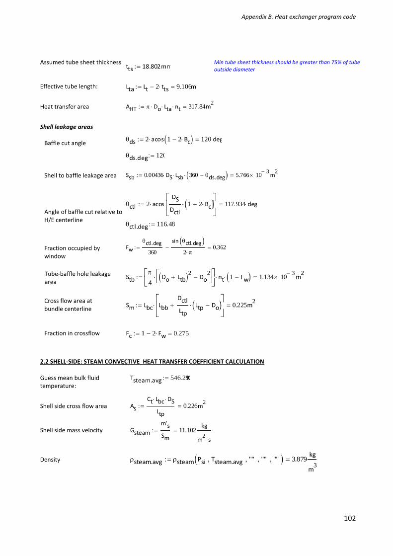
Appendix B. Heat exchanger program code
102
Assumed tube sheet thickness Min tube sheet thickness should be greater than 75% of tube outside diameter
Effective tube length:
Heat transfer area
Shell leakage areas
Baffle cut angle
Shell to baffle leakage area
Angle of baffle cut relative to H/E centerline
Fraction occupied by window
Cross flow area at bundle centerline
Fraction in crossflow
2.2 SHELL-SIDE: STEAM CONVECTIVE HEAT TRANSFER COEFFICIENT CALCULATION
Guess mean bulk fluid temperature:
Shell side cross flow area
Shell side mass velocity
Tube-baffle hole leakage area
Density
tts 18.802mm=
Lta Lt 2 tts− 9.106m==
AHT Do Lta nt 317.84m2
==
ds 2 acos 1 2 Bc−( ) 120 deg==
ds.deg 120=
Ssb 0.00436 DS Lsb 360 ds.deg−( ) 5.766 103−
m2
==
ctl 2 acosDS
Dctl1 2 Bc−( )
117.934 deg==
ctl.deg 116.486=
Fw
ctl.deg
360
sin ctl.deg( )2
− 0.362==
Stb
4Do Ltb+( )2 Do
2−
nt 1 Fw−( ) 1.134 103−
m2
==
Sm Lbc Lbb
Dctl
LtpLtp Do−( )+
0.225m2
==
Fc 1 2 Fw− 0.275==
Tsteam.avg 546.29K=
As
Ct Lbc DS
Ltp0.226m
2==
Gsteam
m's
Sm11.102
kg
m2
s
==
steam.avg steam Psi Tsteam.avg "" "" "" ( ) 3.879kg
m3
==

Appendix B. Heat exchanger program code
103
Kinematic viscosity
Reynolds number
Maximum inter-tube velocity
Specific heat capacity
Prandtl number
Thermal conductivity
Nusselt number
Ideal shell side heat transfer coefficient
Baffle cut correction factor
Baffle cut correction factor
Baffle leakage correction factor
Coefficients
Baffle leakage correction factor
Bundle by-pass, Laminar flow and unequal baffle spacing correction factors
Bundle by-pass correction factor
No flow leakages through pass partition
Unequal spacing correction factor
Baffle spacing is equal
Laminar flow correction factor
Flow in turbulent regime
Actual shell side heat transfer coefficient
steam.avg steam Psi Tsteam.avg "" "" "" "" ( ) 1.906 105−
kg
m s==
steam.wall steam Psi Twall.avg "" "" "" "" ( ) 2.38 105−
kg
m s==
ReS
Gsteam De
steam.avg3.361 10
4==
vmax
m's
steam.avg Sm2.862
m
s==
cp.steam.avg Cpsteam Psi Tsteam.avg "" "" "" "" ( ) 2.158kJ
kg K==
Prsteam.avg Prsteam Psi Tsteam.avg "" ( ) 0.986==
ksteam.avg steam Psi Tsteam.avg "" "" "" "" ( ) 0.042m kg
K s3
==
Nusteam 0.36 ReS0.55
Prsteam.avg
1
3
steam.avg
steam.wall
0.14
107.217==
I
Nusteam ksteam.avg
De77.55
kg
K s3
==
JC 0.55 0.72 1 2 Fw−( )+ 0.748==
rlm
Ssb Stb+
Sm0.031== rs
Ssb
Ssb Stb+0.836==
JL 0.44 1 rs−( ) 1 0.44 1 rs−( )− e2.2− rlm
+ 0.94==
JB 1=
JS 1=
JR 1=
hsteam.corrected I JB JR JS JL JC 54.5kg
K s3
==
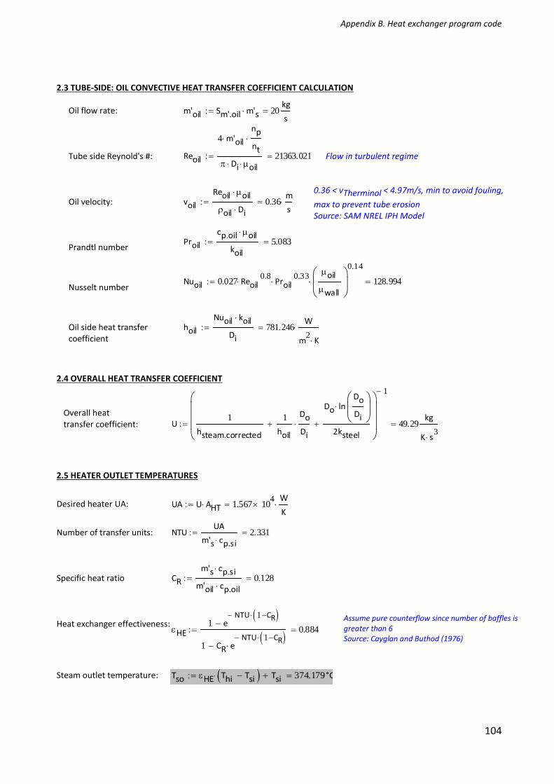
Appendix B. Heat exchanger program code
104
2.3 TUBE-SIDE: OIL CONVECTIVE HEAT TRANSFER COEFFICIENT CALCULATION
Oil flow rate:
Tube side Reynold's #: Flow in turbulent regime
0.36 < vTherminol < 4.97m/s, min to avoid fouling,
max to prevent tube erosion Source: SAM NREL IPH Model
Oil velocity:
Prandtl number
Nusselt number
Oil side heat transfer coefficient
2.4 OVERALL HEAT TRANSFER COEFFICIENT
2.5 HEATER OUTLET TEMPERATURES
Desired heater UA:
Number of transfer units:
Specific heat ratio
Assume pure counterflow since number of baffles is greater than 6 Source: Cayglan and Buthod (1976)
Heat exchanger effectiveness:
Steam outlet temperature:
Overall heat transfer coefficient:
m'oil Sm'.oil m's 20kg
s==
Reoil
4 m'oilnp
nt
Di oil21363.021==
voil
Reoil oil
oil Di0.36
m
s==
Proil
cp.oil oil
koil5.083==
Nuoil 0.027 Reoil0.8
Proil0.33
oil
wall
0.14
128.994==
hoil
Nuoil koil
Di781.246
W
m2
K
==
U1
hsteam.corrected
1
hoil
Do
Di+
Do lnDo
Di
2ksteel+
1−
49.29kg
K s3
==
UA U AHT 1.567 104
W
K==
NTUUA
m's cp.si2.331==
CR
m's cp.si
m'oil cp.oil0.128==
HE1 e
NTU− 1 CR−( )−
1 CR eNTU− 1 CR−( )
−
0.884==
Tso HE Thi Tsi−( ) Tsi+ 374.179°C==

Appendix B. Heat exchanger program code
105
Shell-side fluid mean temperature convergence check
True temperature difference
Heat added to the steam
True temperature difference
Oil outlet temperature
Tube wall temperature convergence check
Calculated HE heat transfer rate
Wall temperature convergence check
3. SHELL & TUBE PRESSURE DROP CALCULATIONS
3.1 TUBE-SIDE: PRESSURE DROP CALCULATION
Isothermal friction factor
Given
Tsteam.avg
Tso Tsi+
2
− 0
Tsteam.calc Tsteam.avg 546.29 K→=
Accuracy steam.temp
Tsteam.calc Tsteam.calc Tsteam.avg−−
Tsteam.calc100 %==
QHE m's cp.steam.avg Tso Tsi−( ) 1.06 MW==
T true
Tso Tsi−
UA
m's cp.steam.avg
67.678K==
Tho Thi
T true UA
m'oil cp.oil− 379.797 °C==
QHE.calc U AHT T true 1.06 MW==
Toil.avg
Tho Thi+
2389.898 °C==
Given
Twall.avg Toil.avg QHE.calc1
hoil AHT−
− 0
Twall.calc Twall.avg 658.084K→=
Accuracy wall.temp
Twall.calc Twall.calc Twall.avg−−
Twall.calc100 %==
fisotherm 0.025=H2O 1000
kg
m3
=

Appendix B. Heat exchanger program code
106
Corrected friction factor
Tube flow area:
Tube side mass velocity:
Specific gravity of oil:
Tube head loss:
Return loss:
Total tube side pressure drop
3.2 OIL PUMP DUTY CHECK
Type: Seal less centrifugal pump (magnetic pump)
Specification: Klaus SLM NHO 065-040-315
Pump volumetric flowrate:
Suction head: Tank height adapted from SAM NREL IPH thermal fluid reservoir dimensions
Total pump head:
Pump efficiency:
Pump power:
3.3 SHELL-SIDE: PRESSURE DROP CALCULATION
Assume that the inlet and outlet nozzle pressure drop = 2 velocity heads each
fcorrected
fisotherm
oil
wall
0.140.026==
Atube
nt 0.25 Di2
np0.08m
2==
Gtube
m'oil
Atube250.613
kg
m2
s
==
sg.oil
oil
H2O0.696==
p t
fcorrected voil2
Lt
Di 2 g0.126m==
p tr
4 np voil2
sg.oil 2 g0.038m==
p tube.tot p tr p t+( ) g oil 1.118 kPa==
V'oil.pump
m'oil
oil103.493
m3
hr==
hs 30m=
Hs hs p tr p t+( )+ 30.164m==
pump 60%=
Paux.oil.pump
oil g Hs V'oil.pump
pump9.86 kW==

Appendix B. Heat exchanger program code
107
Ideal shell pressure drop
Shell side friction factor:
Corrected friction factor
Shell side head loss:
Crossflow pressure drop
Cross flow coefficient:
Number of cross flow rows:
Crossflow pressure drop:
Window zone pressure drop
Window zone flow area:
Effective number of cross flow rows
Window zone pressure drop:
End zone pressure drop
Width of by-pass lane between tubes No pass partition
By-pass area
Ratio of by-pass to cross flow area
fS 0.0012=
fS.corrected
fS
steam.avg
steam.wall
0.141.238 10
3−==
p bI
fS.corrected Gsteam2
DS nb 1+( )
De 2 g steam.avg2
g steam.avg 6.752 Pa==
Kf 0.2670.249 10
4
ReS+
0.927 107
ReS2
−0.1 10
11
ReS3
+ 0.333==
Nc
DS 1 2Lbch
DS−
Ltp15.6==
p c Nc Kf1
2steam.avg vmax
2
0.083 kPa==
DS 2.Lbch−
DS0.5==
Sw
DS2
4acos ( ) 1
2−−( )
nt
81 Fc−( ) Do
2− 0.096m
2==
Ncw
0.8 Lbch
Ltp6.24==
p w
2 0.6 Ncw+( ) m's2
2 Sm Sw steam.avg0.213 kPa==
Lpl 0=
Sb Lbc DS Dotl−( ) Lpl+ =
Fsbp
Sb
Sm0.028==
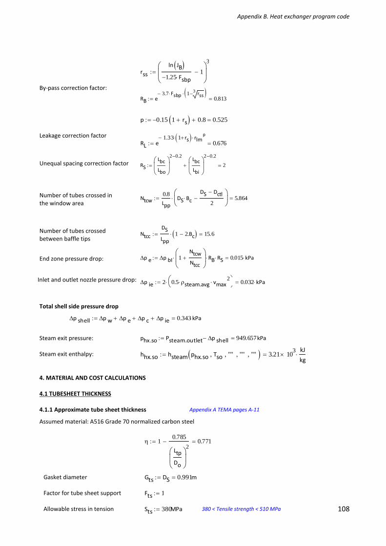
Appendix B. Heat exchanger program code
108
By-pass correction factor:
Leakage correction factor
Unequal spacing correction factor
Number of tubes crossed in the window area
Number of tubes crossed between baffle tips
End zone pressure drop:
Total shell side pressure drop
Steam exit pressure:
Steam exit enthalpy:
4. MATERIAL AND COST CALCULATIONS
4.1 TUBESHEET THICKNESS
4.1.1 Approximate tube sheet thickness Appendix A TEMA pages A-11
Assumed material: A516 Grade 70 normalized carbon steel
Gasket diameter
Factor for tube sheet support
Allowable stress in tension 380 < Tensile strength < 510 MPa
Inlet and outlet nozzle pressure drop:
rss
ln JB( )1.25− Fsbp
1−
3
=
RB e3.7− Fsbp 1
3 rss−( )0.813==
p 0.15− 1 rs+( ) 0.8+ 0.525==
RL e1.33− 1 rs+( ) rlm
p
0.676==
RS
Lbc
Lbo
2 0.2−Lbc
Lbi
2 0.2−
+ 2==
Ntcw0.8
LppDS Bc
DS Dctl−
2−
5.864==
Ntcc
DS
Lpp1 2.Bc−( ) 15.6==
p e p bI 1Ntcw
Ntcc+
RB RS 0.015 kPa==
p ie 2 0.5 steam.avg vmax2
0.032 kPa==
p shell p w p e+ p c+ p ie+ 0.343 kPa==
phx.so Psteam.outlet p shell− 949.657kPa==
hhx.so hsteam phx.so Tso "" "" "" ( ) 3.21 103
kJ
kg==
10.785
Ltp
Do
2− 0.771==
Gts DS 0.991m==
Fts 1=
Sts 380MPa=

Appendix B. Heat exchanger program code
109
Mean metal temperature
Assumed tube sheet thickness (bending):
Assumed tube sheet thickness (shear):
Check if shear or bending is the controlling variable
Variable 1:
Variable 2:
Since << shear will not control, thus design for bending.
4.1.2 Design for bending
Equivalent differential expansion pressure
Elastic modulus:
Elastic modulus tube sheet
Elastic modulus shell
http://asm.matweb.com/search/SpecificMaterial.asp?bassnum=mq304a Elastic modulus of tubes
Coefficient of thermal expansion:
Differential thermal growth between shell and tubes:
Assume there are no shell expansion joints
Coefficients:
Tmean
Twall.calc Tsteam.avg+
2602.187K==
Tts.bending
Fts Gts
3
Psteam.outlet
Sts 18.802 mm==
Tts.shear
0.31 De
1Do
Ltp−
Psteam.outlet
Sts 0.097 mm==
Psteam.outlet
Sts2.5 10
3−=
1.6 1Do
Ltp−
0.736=
Psteam.outlet
Sts1.6 1
Do
Ltp−
E T( ) T T /°C
E 206 4.326− 102−
T+ 3.502 105−
T2
−
1− 6.592 108−
T3
+
E GPa
=
Ets E Tmean( ) 185.626GPa==
Es E Tsteam.avg( ) 190.228GPa==
Et 193GPa=
t 17.2m
m K= s 12
m
m K=
L Lta s Tsteam.avg 70 °F−( )
1− t Toil.avg 70 °F−( )+
30.222− mm==
Jts 1=
Kts
Es ts DSO ts−( )
Et t nt Do t−( )0.637==

Appendix B. Heat exchanger program code
110
Differential expansion pressure:
Effective shell side design pressure
Shell equivalent pressure:
Effective shell design pressure: Shell design pressure sufficient to withstand operating conditions
Effective tube side design pressure
Oil pressure:
Tube equivalent pressure:
Effective tube design pressure:
Tube sheet thickness convergence check
Actual tube sheet standard thickness:
Fq 0.25 Fts 0.6−( )300 ts Es
Kts Lta Ets
Gts
Tts.bending
3
1
4
+ 7.547==
Pd
4 Es tsL
Lt
DSO 3 ts−( ) 1 Jts Kts Fq+( )6.339− 10
3 kPa==
P's Psteam.outlet
0.4 Jts 1.5 Kts 1.5 1 nt
Do
Gts−
+
+
1 Jts Kts Fq+
=
PS
P's Pd−
23.037 MPa==
Poil oil g Hs 205.792kPa==
P't Poil
1 0.4 Jts Kts 1.5 1 nt
Do 2 t−
Gts
2
−
+
+
1 Jts Kts Fq+
=
Pt P't P's− 322.276kPa==
Given
tts
Fts Gts
3
Psteam.outlet
Sts
− 0
Tts.calc Find tts( ) 18.802 mm==
Accuracy ts.thickness
Tts.calc Tts.calc tts−−
Tts.calc99.998 %==
tts.actual 20mm=

Appendix B. Heat exchanger program code
111
4.2 DESIGN OF HEAT EXCHANGER INLET & OUTLET NOZZLE AND ENDS
Check if it is a thin/ thick cylinder
Since d/t >> 20 the cylinder is a thick cylinder
Design for a thick-walled cylinder, type E shell
External pressure:
Internal pressure: Effective design internal pressure = 110% of operating pressure (Richard & Coulson Vol.6)
Internal radius:
External radius:
Lame's constants:
Lame' constants:
Longitudinal stress in shell:
Mean shell radius:
Radial stress in shell:
Select boiler steel for shell material A516 Grade 70 normalized steel Hoop stress in shell:
4.2.1 Selection of heat exchanger ends
Cylindrical section plate thickness:
Option 1: Torri spherical shape
DS
ts69.273=
P2 1atm=
P1 1.1 Psteam.outlet=
R1 DS 0.5 0.495m==
R2 R1 ts+ 0.51m==
AL.guess 50= BL.guess 13=
Given
AL.guess
BL.guess
R1
m
2−
P1−
Pa AL.guess
BL.guess
R2
m
2−
P2−
Pa
Constants Find AL.guess BL.guess ( )1.601 10
7
4.184 106
==
AL Constants0
Pa 16.009 MPa==
BL Constants1
N 4.184 MN==
L
P1 R12
P2 R22
−
R22
R12
−
16.009 MPa==
r 0.5 R1 R2+( ) 0.502m==
r AL
BL
r2
− 0.563− MPa==
H AL
BL
r2
+ 32.581 MPa==
edesign ts 14.3 mm==
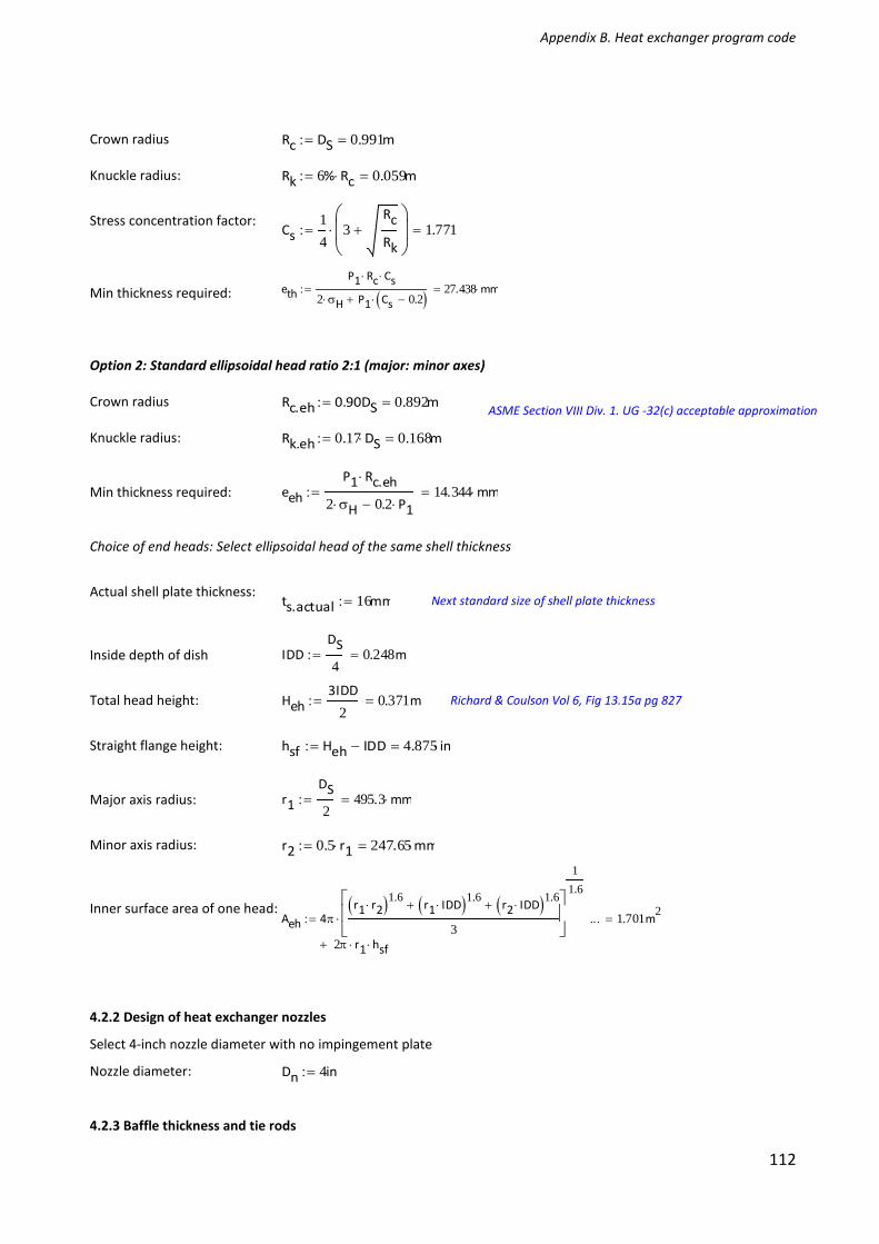
Appendix B. Heat exchanger program code
112
Crown radius
Knuckle radius:
Stress concentration factor:
Min thickness required:
Option 2: Standard ellipsoidal head ratio 2:1 (major: minor axes)
Crown radius ASME Section VIII Div. 1. UG -32(c) acceptable approximation
Knuckle radius:
Min thickness required:
Choice of end heads: Select ellipsoidal head of the same shell thickness
Actual shell plate thickness: Next standard size of shell plate thickness
Inside depth of dish
Total head height: Richard & Coulson Vol 6, Fig 13.15a pg 827
Straight flange height:
Major axis radius:
Minor axis radius:
Inner surface area of one head:
4.2.2 Design of heat exchanger nozzles
Select 4-inch nozzle diameter with no impingement plate
Nozzle diameter:
4.2.3 Baffle thickness and tie rods
Rc DS 0.991m==
Rk 6% Rc 0.059m==
Cs1
43
Rc
Rk+
1.771==
eth
P1 Rc Cs
2 H P1 Cs 0.2−( )+27.438 mm==
Rc.eh 0.90DS 0.892m==
Rk.eh 0.17 DS 0.168m==
eeh
P1 Rc.eh
2 H 0.2 P1−14.344 mm==
ts.actual 16mm=
IDDDS
40.248m==
Heh3IDD
20.371m==
hsf Heh IDD− 4.875 in==
r1
DS
2495.3 mm==
r2 0.5 r1 247.65 mm==
Aeh 4r1 r2( )1.6
r1 IDD( )1.6+ r2 IDD( )1.6
+
3
1
1.6
2 r1 hsf+
1.701m2
==
Dn 4in=

Appendix B. Heat exchanger program code
113
Tie rod diameter: Table CB-4.71 TEMA 9th Edition
Number of tie rods:
Unsupported tube length between baffles:
Baffle plate thickness: Table CB-4.41 TEMA 9th Edition
Actual baffle thickness:
4.3 MASS OF METAL REQUIRED
NB: All steel calculations were based on Aveng Trident Steel prices and specifications. Boiler steel was used for the shell and baffle plates and stainless-steel tubes.
4.3.1 Shell calculations: Including baffles
Density of boiler steel
Multiplying factor:
Cylindrical section:
Base perimeter
Mass of cylinder:
Front and rear end heads:
Volume of each end:
Mass of steel:
Total mass for front and rear ends:
Tube sheet:
Total volume required:
Total mass of steel:
Actual thickness:
Select standard width:
Calculated length: Add 5% for cutting tolerance
Dt 12.7mm=
ntr 8=
Lbu
Lta
nb479.284 mm==
tb.min 6.4mm=
tb ceiltb.min
mm
mm 7 mm==
bs 7861kg
m3
=
MF 7.85=
LPS DS 3.112m==
mcylinder LPS Lt ts bs 3.199 tonne==
Veh4
3 r1 r2 IDD r1
2 hsf+ 222.675L==
mhead bs Veh 1.75 103
kg==
mtot.head 2 mhead 3.501 tonne==
Vts r12
tts.actual 2 30.828L==
mtubesheets bs Vts 242.34kg==
tts.actual 20 mm=
wplate.ts 1200mm=
lplate 1.05mtubesheets
wplate.ts bs tts.actual1.349m==

Appendix B. Heat exchanger program code
114
Baffles:
Total volume required:
Total mass of steel:
Actual thickness:
Select standard width:
Calculated length:
4.3.2 Tube bundle calculations
Tube material: ASTM A312 Stainless steel, schedule 40S, Grade TP304 fusion welded (dimensions based on ANSI B36.10)
Total number of tubes:
Tube length:
Nominal pipe size:
Tube thickness:
Density of stainless steel:
Total mass of steel:
4.4 HEAT EXCHANGER MATERIAL COSTS
Cost per tonne:
Boiler steel: Estimated Aveng Steel last known price
Stainless steel: Confirmed Euro Steel price
Total mass of steel
Boiler steel:
Stainless steel:
Total H/E steel cost:
Total cost of H/E:
Vb 1 Bc−( ) r12
tb nb 76.878L==
mbaffles bs Vb 604.334kg==
tb.actual 8mm=
wplate 2400mm=
lplate.baffles 1.05mbaffles
wplate bs tb.actual4.204m==
nt 648=
Lt 30 ft=
NPS3
8in=
t 0.091 in=
ss 8070kg
m3
=
mtubebundle nt Di Lt t ss 4.348 tonne==
Cbs10000¤
tonne=
Css125¤
m=
mtot.bs mbaffles mtubesheets+ mtot.head+ mcylinder+ 7.546 tonne==
mtot.ss mtubebundle 4.348 tonne==
Coststeel mtot.bs Cbs Css nt Lt+ 816128.54ZAR==
HEcost Coststeel 1.5 1224192.81ZAR==

Appendix B. Heat exchanger program code
115
0
RESULTS
5.0 RESULTS
Heat exchanger spec: Type BEM Size 39 - 360 (991-9144)
Total heat transfer area:
Steam heat addition:
H/E effectiveness:
Cost of H/E:
Steam outlet temperature:
Steam exit enthalpy:
AHT 317.84m2
=
QHE 1.06 MW=
HE 88.386 %=
HEcost 1224192.81ZAR=
Tso 374.179°C=
hhx.so 3210.39kJ
kg=

Appendix C. Turbine quote
116
Appendix C. Turbine calculations program code
1.TURBINE OUTPUT
Property data: Plant specifications
Plant capacity
Process steam requirements:
Load rating:
Specification: Siemens SST -060 Turbine- Alternator set
1.1 GENERATOR INPUT SHAFT POWER: FULL LOAD REQUIREMENTS
Turbo-alternator efficiency
Generator output apparent power
Generator efficiency
Generator input power
1.2 TURBINE INLET STEAM CONDITIONS: FULL LOAD
Turbine efficiency
Turbine power
Assuming 5% pressure drop in the steam lines and governing valves:
Extraction line pressure drop
Turbine exhaust pressure
Steam header input to turbine
Boiler 1 & 2 exit pressure
Reference:C:\Research\Water-Steam IAPWS-IF97 rev 1.2.xmcd
Reference:C:\Research\HEAT EXCHANGER DETAILED DESIGN.xmcd
PCAP 46 106
L
yr=
pplant 400kPa= Tplant 100°C=
hplant hsteam pplant Tplant "" "" "" ( ) 419.32kJ
kg==
Pload 621.68kW= PF 0.85=
ta 86%=
Qoutput
Pload
PF731388.24V A==
gen 95%=
Pin.gen
Pload
gen654.4 kW==
turb
ta
gen90.53 %==
Pturb.required
Pin.gen
turb722.88 kW==
p loss 5%=
pout pplant 1 p loss+( )( ) 420 kPa==
pboiler 950kPa=

Appendix C. Turbine quote
117
Steam header pressure
Turbine inlet pressure
1.3 TURBINE ACTUAL OUTPUT POWER
Assumed turbine inlet temp
Turbine inlet quality
Turbine inlet enthalpy
Turbine exit enthalpy
Turbine exit temperature
Turbine exit quality
1.4 OIL PUMP AUXILLIARY POWER REQUIREMENTS & SOP
Pump power:
Fraction of turbine output:
Sent out power
Imported power:
1.5 MASS FLOW REQUIRED TO MEET PLANT POWER REQUIREMENT
Turbine work:
Mass flow required:
% increase in mass flow:
pheader pboiler p shell− 949657.44Pa==
pturb.in pheader 1 p loss−( ) 902174.57Pa==
Tin Tsteam pturb.in "" hhx.so "" ( ) 646.93K==
xin xsteam pturb.in Tin "" "" "" ( ) 1.22==
hin hsteam pturb.in Tin "" "" "" ( ) 3210.39kJ
kg==
sin ssteam pturb.in Tin "" "" "" ( ) 7.43kJ
kg K==
hex.s hsteam pout "" "" "" sin ( )=
hex hin turb hin hex.s−( )− 3023.33kJ
kg==
Pturb m'in hin hex−( ) 467.65 kW==
hexit hin
Pturb
m'in− 3023.33
kJ
kg==
Texit Tsteam pout "" hexit "" ( ) 278.92 °C==
xexit xsteam pout "" "" hexit "" ( ) 1.13==
Paux.oil.pump 9.86 kW=
faux
Paux.oil.pump
Pturb2.11 %==
PSOP 1 faux−( ) Pturb 457.79 kW==
Pimport Pturb.required Pturb− 255.24kW==
wturb hin hexit− 187.06kJ
kg==
m'req
Pturb.required
wturb13.91
tonne
hr==
%mf
m'req m'in−
m'in54.58%==

Appendix C. Turbine quote
118
Appendix D. Turbine Quote
NB: Efforts to get the current quote were unfruitful and the researcher used the last known price
obtained in 2016 during the researcher’s undergraduate research.