soil landscape reconnaissance mapping · soil landscape reconnaissance mapping nsw western regional...
TRANSCRIPT

SSooiill LLaannddssccaappeeRReeccoonnnnaaiissssaanncceeMMaappppiinngg
NNSSWW WWEESSTTEERRNN RREEGGIIOONNAALLAASSSSEESSSSMMEENNTTSS
FFIINNAALL RREEPPOORRTT JJUUNNEE 22000022
Resource and ConservationAssessment Council
Brigalow BeltSouth
Stage 2


Soil Landscape ReconnaissanceMapping�Brigalow Belt South (BBS)Interim Bioregion
NNSSWW WWEESSTTEERRNN RREEGGIIOONNAALL AASSSSEESSSSMMEENNTTSS
FFIINNAALL RREEPPOORRTT JJUUNNEE 22000022
A project undertaken for the Western Regional Assessment of NSWfor the Resource and Conservation Assessment CommitteeProject number: WRA 21
NEW SOUTH WALES GOVERNMENT

Soil Landscape Reconnaissance Project - Brigalow Belt South Interim Bioregion (WRA)ii
For more information and access to data contact:Resource and Conservation DivisionPlanning NSWGPO Box 3927SYDNEY NSW 2001Phone: (02) 9762 8207
Department of Land and Water ConservationSoil Information Systems [email protected] Box 3720PARRAMATTA NSW 2124Phone: (02) 9895 6172
© New South Wales GovernmentJune 2002
This document should be cited as:
Soil Information Systems Unit (2002), Soil Landscape Reconnaissance Mapping - Brigalow BeltSouth Stage 2, Department of Land and Water Conservation, Sydney, NSW.
ISBN 1 74029 181 6
Soil Landscape Reconnaissance Project - Brigalow Belt South Interim Bioregion (WRA) iii
CONTRIBUTIONS AND ACKNOWLEDGMENTS
This program was funded by the New South Wales Government and managed through the Resourceand Conservation Division, Department of Urban Affairs and Planning (DUAP). Thanks go to RicNoble, John Ross and Emma Mason for their advice and assistance with many aspects of this project.
Many Department of Land and Water Conservation (DLWC) staff also contributed to this project andtheir efforts are greatly appreciated. The following soil surveyors provided soil survey and soilattribute data for the project: Rob Banks, Karl Andersson, Mark Blair, Brian Jenkins, Brian Murphy,Dacre King and Evan Pengelly. Katie-Jane Nixon, Mark Young, Nicole Simons, Kate Secombe andAlex McGaw provided technical assistance.
Thanks also go to Ross Beasley, Jeremy Black, Jeanine Murray, Gary Coady and Paul Wettin formaking staff available for this project and to the Barwon Region’s Resource Information Unit (RIU),in particular their GIS unit, for the provision of spatial information and expertise.
Simon Ferrier and his team at National Parks and Wildlife Service (NPWS) provided importanttechnical advice on gap analysis and provided their code for use in the flexible gap analysis tooldeveloped by Dr. Geoff Goldrick.
Special thanks are extended to Dr. Geoff Goldrick who set-up and produced a series of sophisticatedsoil landscape maps using geographic information and statistical modelling systems, as well asdeveloping the flexible gap analysis software. This project could not have been completed withouthis significant inputs. Geoff received assistance in constructing the GIS modelling environment fromPaul Rampant at the Centre for Land Protection (Bendigo, Victoria) and Neil McKenzie, ChrisMoran, John Gallant and Elizabeth Bui from CSIRO Division of Land and Water.
DLWC's Barwon Region Resource Information Unit and the NSW Department of Mineral Resourcesprovided many of the underlying datasets.
Casey Murphy, Katie-Jane Nixon, Alex McGaw, Nicole Simons and Mark Young constructed andpopulated the database, with Nicole preparing the accompanying user guide. They also loaded soilprofile information into the NSW Soil and Land Information System (SALIS), and calculated manyof the soil attributes. Jonathan Gray provided the lithology classification used in the database. MarkYoung, Andrew Murrell and Hugh Jones completed the model accuracy checks.
Special thanks are also extended to Leanne Wallace, Peter Gallagher and Dorothy Mullins for theiradvice and support, within both DLWC and the WRA steering committee.
This project was initiated and managed by Greg Chapman, with technical supervision and qualitycontrol provided by Greg Chapman, Casey Murphy and Brian Jenkins.
This report is presented as per those prepared for previous Comprehensive Regional Assessments. Italso builds on work presented in Goldrick et al. 2001. The report was written by Greg Chapman andwas edited by Anne Bell, Brian Jenkins, Humphrey Milford, Casey Murphy, Mark Young andAndrew Murrell.
DISCLAIMER
Reconnaissance soil landscape mapping undertaken by DLWC constituted one of the largestquantitative land resource assessments undertaken to date in NSW. Every reasonable effort has beenmade to ensure that the mapping and information related to this project is correct. The State of NewSouth Wales, its agents and employees do not assume any responsibility and shall have no liability,consequential or otherwise of any kind arising from the use of or reliance on any of the informationcontained in the maps, this document or any other information related to this project.

Soil Landscape Reconnaissance Project - Brigalow Belt South Interim Bioregion (WRA)iv
1 Executive Summary....................................................................................................................................... 1
1.1 What has been provided? ...................................................................................................................... 1
1.2 How was it done?.................................................................................................................................. 1
1.3 What are the products? ......................................................................................................................... 2
2 Introduction ................................................................................................................................................... 4
2.1 Background ........................................................................................................................................... 4
2.1.1 The Brigalow Belt South Interim Bioregion ..................................................................................... 4
2.1.2 Study rationale .................................................................................................................................. 5
2.2 Project Objectives ................................................................................................................................. 6
3 Methods .......................................................................................................................................................... 7
3.1 Scope of Project .................................................................................................................................... 7
3.1.1 Project planning and management .................................................................................................... 7
3.1.2 Why the geographic statistical modelling approach was used .......................................................... 8
3.1.3 Project variation................................................................................................................................ 8
3.1.4 What is a soil landscape? .................................................................................................................. 9
3.2 Existing Datasets................................................................................................................................. 10
3.2.1 Soil landscape maps........................................................................................................................ 10
3.2.2 Soil profile point data ..................................................................................................................... 11
3.3 Calculation of key soil attributes ........................................................................................................ 11
3.3.1 Modified fertility class .................................................................................................................... 12
3.3.2 Drainage.......................................................................................................................................... 14
3.3.3 Effective rooting depth ................................................................................................................... 14
3.3.4 Estimated plant available water holding capacity ........................................................................... 15
3.4 Analysis ............................................................................................................................................... 18
3.4.1 Geographic modelling tools ............................................................................................................ 18
3.4.2 Soil landscape description recording .............................................................................................. 19
4 Work Program............................................................................................................................................. 20
4.1 Project Set-Up phase .......................................................................................................................... 20
4.2 Training Area Phase ........................................................................................................................... 20
4.3 Main Fieldwork And Modelling Phase ............................................................................................... 20
4.4 Post fieldwork phase ........................................................................................................................... 21

Soil Landscape Reconnaissance Project - Brigalow Belt South Interim Bioregion (WRA) v
5 Project Tasks................................................................................................................................................ 22
5.1 Project Set-up Phase........................................................................................................................... 22
5.1.1 Marshall staff, initial training, obtain specialist software and equipment ....................................... 22
5.1.2 Literature search and entry of existing soil profiles to SALIS ........................................................ 22
5.1.3 Establish map unit string................................................................................................................. 225.1.3.1 Provinces................................................................................................................................ 235.1.3.2 Lithology code ....................................................................................................................... 235.1.3.3 Modal slope code ................................................................................................................... 265.1.3.4 Landform pattern or element code ......................................................................................... 265.1.3.5 Soil landscape code................................................................................................................ 265.1.3.6 Facet code .............................................................................................................................. 26
5.1.4 Build MS Access database for soil landscape descriptions............................................................. 27
5.1.5 Build WRA Soil Data Card for SALIS with appropriate fields for western soil conditions ........... 30
5.1.6 Soil profile attribute data entry to SALIS ....................................................................................... 32
5.1.7 Assemble predictor surfaces and prepare predictor surfaces for proto-soil landscape modelling... 32
5.1.8 Predictor variable preparation......................................................................................................... 35
5.1.9 Initial data modelling ...................................................................................................................... 35
5.1.10 Cross-validation.......................................................................................................................... 375.1.10.1 Tree ‘pruning’ to reduce complexity...................................................................................... 38
5.1.11 Smoothing of the output prediction surfaces to become maps.................................................... 39
5.1.12 Initial model evaluation .............................................................................................................. 39
5.2 Training Area Phase ........................................................................................................................... 39
5.2.1 Compilation of independent checking dataset................................................................................. 39
5.2.2 Staff briefing and work allocation................................................................................................... 39
5.2.3 Training area selection.................................................................................................................... 41
5.2.4 Training area pre-field preparations................................................................................................ 41
5.2.5 Training area fieldwork................................................................................................................... 41
5.2.6 Training area digitising and database entry..................................................................................... 41
5.3 Main Fieldwork and Modelling Phase................................................................................................ 42
5.3.1 Post-training area modelling and model iterations.......................................................................... 43
5.3.2 Modelling by province and weighting of modelling within provinces ............................................ 435.3.2.1 Liverpool Ranges ................................................................................................................... 435.3.2.2 Liverpool Plains ..................................................................................................................... 435.3.2.3 Talbragar Valley .................................................................................................................... 435.3.2.4 Pilliga Outwash ...................................................................................................................... 445.3.2.5 Pilliga ..................................................................................................................................... 445.3.2.6 Northern Basalts..................................................................................................................... 455.3.2.7 Northern Outwash .................................................................................................................. 45
5.3.3 Site selection and gap analysis ........................................................................................................ 45
5.3.4 Gap analysis .................................................................................................................................... 46

Soil Landscape Reconnaissance Project - Brigalow Belt South Interim Bioregion (WRA)vi
5.3.5 Flexible gap analysis....................................................................................................................... 47
5.3.6 Main fieldwork................................................................................................................................ 48
5.3.7 Landholder communication protocols............................................................................................. 49
5.4 Post Fieldwork .................................................................................................................................... 49
5.4.1 Final modelling ............................................................................................................................... 49
5.4.2 Province boundary adjustments ...................................................................................................... 49
5.4.3 Line work adjustments .................................................................................................................... 49
5.4.4 Polygon tag changes........................................................................................................................ 50
5.4.5 Soil profile point data gaps ............................................................................................................. 50
5.4.6 Soil landscape database gaps .......................................................................................................... 50
5.4.7 “Mopping up” fieldwork................................................................................................................. 50
5.4.8 Linkage of soil landscape polygons and database........................................................................... 51
5.4.9 Attribution of soil landscape spatial summary parameters.............................................................. 515.4.9.1 Terrain attributes .................................................................................................................... 515.4.9.2 Temperature attributes ........................................................................................................... 51
5.4.10 Database attribution with major variables and calculation of key soil attributes ........................ 52
5.4.11 Map and database checking........................................................................................................ 525.4.11.1 Visual comparison of the model with its source maps ........................................................... 525.4.11.2 Logical consistency checking................................................................................................. 525.4.11.3 Misclassification checking ..................................................................................................... 535.4.11.4 Evaluation against the independent dataset ............................................................................ 535.4.11.5 Evaluation of training area representativeness ....................................................................... 54
5.4.12 Allocation of soil landscapes to 15 km buffer ............................................................................ 54
5.4.13 Design of Web products ............................................................................................................. 54
5.4.14 Access to information................................................................................................................. 54
5.4.15 Feedback..................................................................................................................................... 55
6 Outputs ......................................................................................................................................................... 56
6.1 Soil profile information ....................................................................................................................... 56
6.2 Map coverages and database.............................................................................................................. 56
6.2.1 Soil landscape coverage.................................................................................................................. 56
6.2.2 Other coverages .............................................................................................................................. 56
6.3 Soil attribute themes............................................................................................................................ 56
6.4 Soil landscape database...................................................................................................................... 57
6.5 Use of data .......................................................................................................................................... 57
6.6 Metadata ............................................................................................................................................. 57
6.7 Overlays .............................................................................................................................................. 58
7 Discussion ..................................................................................................................................................... 59
7.1 Are the data and conclusions robust and reliable?............................................................................. 59
7.2 How do the outputs from this process compare with other soil landscape mapping projects? .......... 59

Soil Landscape Reconnaissance Project - Brigalow Belt South Interim Bioregion (WRA) vii
7.3 Was the project variation successful? ................................................................................................. 59
7.4 How will the project be useful to the assessment? .............................................................................. 60
7.5 Model testing accuracy ....................................................................................................................... 60
7.5.1 Distribution and Descriptive Statistics............................................................................................ 60
7.5.2 Cohen’s Kappa................................................................................................................................ 66
7.5.3 Synthesis and Conclusion of Accuracy Tests.................................................................................. 67
8 Appendices ................................................................................................................................................... 69
8.1 Appendix 1: Western Regional Assessment Soil Data card ................................................................70
8.2 Appendix 2: References....................................................................................................................... 72
8.3 Appendix 3: Maps ............................................................................................................................... 75
Figures
Figure 1: Location and extent of the Brigalow Belt South Interim Bioregion ........................................................ 4Figure 2: Diagrammatic representation of the use of regression models for predicting soil-landscape units.......... 9Figure 3: Cross-section of a soil landscape showing the relationship between the soil landscape and its facetsafter Charman (1978)............................................................................................................................................ 12Figure 4: The calculation of estimated rooting depth ........................................................................................... 14Figure 5: Extent of existing 1:100,000 (yellow) and 1:250,000 (blue) soil landscape mapping in the BBS ........ 36Figure 6: A partial classification tree (upper nodes and branches) from the RPART analyses of the training dataincluding radiometrics for the BBS indicating the decision criteria ..................................................................... 37Figure 7: The relationship between tree complexity and cross-validation error for the classification trees of theBBS based on radiometrics................................................................................................................................... 38Figure 8: Grid of predicted soil landscapes as initially modelled for the south-eastern portion of the BBS (a) anddetail of a section with overlay of the training data line work (b)......................................................................... 39Figure 9: Detail of area around Narrabri illustrating the usefulness of the REI for identifying levees anddepressions ........................................................................................................................................................... 42Figure 10: Three data points in the two-dimensional environmental space defined by precipitation and elevation.............................................................................................................................................................................. 46Figure 11: Estimates of the average distance in environmental space of all grid cells in the BBS from the pointsin the training data (excluding lithology and radiometric data) ............................................................................ 47Figure 12: A soil corer in use on the gently undulating plains of the Northern Outwash...................................... 48Figure 13: Percentage accuracy for topsoil texture across all provinces............................................................... 62Figure 14: Percentage accuracy for Effective Rooting Depth across all provinces............................................... 62Figure 15: Percentage accuracy for Regolith across all provinces........................................................................ 63Figure 16: Percentage accuracy for EPAWC across all provinces ....................................................................... 63Figure 17: Percentage accuracy for Fertility across all provinces......................................................................... 64Figure 18: Percentage distribution of results showing percentage of matches for all for all main attributes fromeach province as a score out of 5. ......................................................................................................................... 64

Soil Landscape Reconnaissance Project - Brigalow Belt South Interim Bioregion (WRA)viii
Tables
Table 1: Fertility classes of Great Soil Groups ..................................................................................................... 12Table 2: Estimated plant available water holding capacity (EPAWC) values for texture grades ......................... 15Table 3: The GIS software packages and their functions...................................................................................... 19Table 4: Map unit and facet string layout ............................................................................................................. 23Table 5: Table listing types and codes for lithology used in the map string ......................................................... 24Table 6: Soil and landscape properties recorded for each soil landscape unit in the MS Access database........... 27Table 7: Facet properties recorded for each soil landscape unit in the MS Access database................................ 29Table 8: Site and soil attributes recorded on WRA Soil Data Cards .................................................................... 31Table 9: Base datasets used in the BBS study and their potential uses................................................................ 33Table 10: The environmental parameters (predictor variables) used for modelling and prediction of soillandscapes in the BBS .......................................................................................................................................... 34Table 11: Effective Rooting Depth ranges for calculation of accuracy ................................................................ 60Table 12: EPAWC ranges for calculation of accuracy ......................................................................................... 60Table 13: Fertility ranges for calculation of accuracy........................................................................................... 60Table 14: A1 Texture ranges for calculation of accuracy ..................................................................................... 61Table 15: Regolith ranges for calculation of accuracy.......................................................................................... 61Table 16: Liverpool Plains province descriptive statistics for each of the test parameters. .................................. 65Table 17: Northern Basalts province descriptive statistic of each of the test........................................................ 65Table 18:Northern Outwash province descriptive statistic for each of the test parameters................................... 65Table 19: Pilliga province descriptive statistic for each of the test parameters ................................................... 65Table 20:Pilliga Outwash Descriptive Statistic for each of the test parameters.................................................... 66Table 21:Accuracy for each of the provinces for all five parameters expressed as a percentage.......................... 66Table 22: Strength of Agreement ratings for Cohens Kappa Statistic .................................................................. 67Table 23: Summary of agreement statistics for the five soil characteristics.......................................................... 67
Soil Landscape Reconnaissance Project - Brigalow Belt South Interim Bioregion (WRA) 1
1.1 WHAT HAS BEEN PROVIDED?
The NSW Department of Land and Water Conservation (DLWC) has provided reconnaissance-levelsoil landscape mapping and soil attribute information for the Brigalow Belt South (BBS) InterimBioregion, an area of approximately 52,400km2. This information is to be used in native vegetationmapping and to assist with the determination of soil and land capability for public land use allocation.
Starting in late January 2001, and with datasets made available in February 2002, this projectprovided fundamental soil and other biophysical attribute data for many modelling projects within theNSW Western Regional Assessment process. These projects include assessments of the distributionof individual plant and animal species, the extent and pre-European distribution of vegetationcommunities, and site quality and associated fertility for timber resources. Furthermore, this projectprovided information concerning soil properties and limitations that will prove useful for sustainableland use planning.
1.2 HOW WAS IT DONE?
Innovative computer modelling methods were used to map the BBS in a more rapid, quantitative andrepeatable manner than could be achieved by using traditional reconnaissance land resource mappingmethods. In the southern portion of the mapping area the technique used involved recursivepartitioning of available environmental variables trained on existing soil landscape mapping todevelop rules for allocating soil mapping classes to adjacent areas. The environmental variablesincluded digital elevation models (DEMs) and climate interpolative drapes as well as geology andsoil parent material maps and gamma radiometric imagery.
In the northern and western parts of the BBS, where soils information was not available, nine smallertraining areas were chosen for representative soil mapping, which was then modelled throughoutthose areas based on the rules developed in the training areas.
Several key environmental variables such as surface geology and gamma radiometrics were neithercontinuous nor wholly available at the time of survey, which hampered modelling progress.Combined with limited digital elevation information in areas of lowest relief in the west of the studyarea, this presented challenges that need to be addressed before starting similar surveys.
Initial outputs from the model were originally applied universally over the entire area. It was found,however, that this over-represented the landscape-forming processes that dominate the south-easternpart of the study area but are not as prevalent elsewhere. The study area was subsequently subdividedinto seven provinces. This allowed geographic differences in landscape and soil formation processesin the bioregion to be modelled individually. This approach was adjusted with further refining ofprovince boundaries and subdivision of mapping areas for individual modelling.
Training area information, and other compiled soil data, were used for iterative refining of the soilsmap over the remainder of the area by using various combinations of repeated recursive partitioning.
Advice on model success or otherwise was only possible using critical feedback from the soilsurveyors and technical officers who extensively sampled soils and landscape conditions in the study

Soil Landscape Reconnaissance Project - Brigalow Belt South Interim Bioregion (WRA)2
area. Location of sampling points was guided by the use of a flexible gap analysis software packagerunning on laptop computers. The model-feedback approach was developed, in some cases, down toindividual soil landscapes. In some areas, the model was modified more than eight times until furtherimprovement could not be obtained within the constraints of the project. In some instances, modellingreverted to the use of radiometrics classifications, existing mapping and hand-drawn polygonsbecause the available environmental variables could not sufficiently delineate soil boundaries.
A smoothing and editing process was employed to resolve edge matches caused by discontinuities inthe environmental surfaces.
Mapping was conducted at a technical standard consistent with national agreements and standardsdeveloped under the Australian Collaborative Land Evaluation Program (ACLEP) by DLWC’s SoilSurvey Unit team of trained and qualified soil surveyors.
Soil and land descriptions follow the guidelines of the Soil and Land Survey Field Handbook(Macdonald et al. 1990). Soil and land data collection used a combination of integrated and free soilsurvey and is a synthesis of methods outlined in the Australian Soil and Land Survey Handbook—Guidelines to Conducting Surveys (Gunn et al. 1988), with the exception of the 15 km buffer.
The map unit database was joined with map coverage to enable various soil and landscape parametersto be portrayed.
1.3 WHAT ARE THE PRODUCTS?
Over 3,500 soil profiles were collected from existing records or described as part of this project andentered into DLWC’s NSW Soil And Land Information System (SALIS). This compares with around1,300 soil profile records available for the area at the start of the project. An independent samplingset, which is being finalised, will feature around 80 sites taken from the same locations as fauna andflora descriptions. This data will be valuable for double-checking against vegetation mappingpredictions.
The main product is a reconnaissance Soil Landscape Map for use in Geographic Information System(GIS) format. Each mapping unit is linked to a corresponding record in an MS Access database. Mainattributes include:
� Soil type;
� Soil depth;
� Drainage;
� Estimated rooting depth;
� Fertility;
� Estimated plant available water capacity; and
� Soil regolith stability class.
Further, each map unit has been assessed for localised or widespread presence of:
� Seasonal waterlogging, flood hazard, high run-on, groundwater pollution hazard;
� Gully erosion risk, sheet erosion risk, wind erosion hazard;
� Shallow Soil, non-cohesive soil, complex soil;
� Seepage scalds, saline discharge, potential recharge;
� Foundation hazard, surface movement potential; and

Soil Landscape Reconnaissance Project - Brigalow Belt South Interim Bioregion (WRA) 3
� Steep slopes, mass movement hazard.
Soil attribute information can be linked to Digital Elevation Models (DEMs) to produce a higherresolution of soil attributes at more intense scales.
A feature of the project was the use of 180 stratified random soil profiles to compare with predictionsof the mapped surfaces. For the five major attributes tested the mapping was found to be correct tocategory level in more than 70% of cases. Soil Landscape mapping which is almost three times moreexpensive is expected to be accurate to category level in 85% of cases
Beyond the scope of this project, DLWC undertakes to make these and other map views availableover the Internet in the future.
This mapping is provided at reconnaissance level and should be used only as a guide to thedistribution of specific soil attributes identified for the purposes of this project.

Soil Landscape Reconnaissance Project - Brigalow Belt South Interim Bioregion (WRA)4
2.1 BACKGROUND
This report describes a project undertaken as part of the Western Regional Assessments (WRA's) ofpublic lands in western NSW. The WRA's provide the scientific basis on which rational decisions aremade to determine the best use of public land in western NSW. The Western Regional Assessmentprocess is based on consecutive assessment of specified target areas.
The Brigalow Belt South (BBS) project is the second WRA project area. It follows Stage 1assessments in forests in the east of the Southern Brigalow Interim Bioregion. Future assessmentareas are likely to include land in the Nandewar and New England Tableland Interim Bioregions thatwere not studied as part of the North-East Comprehensive Regional Assessment (CRA) undertaken in1997.
2.1.1 The Brigalow Belt South Interim Bioregion
The Brigalow Belt South Interim Bioregion (BBS) covers over 52,400km2, or 6.2% of NSW. Itextends from the Queensland border south to Narromine and east to Merriwa (see Figure 1).Gunnedah, Coonabarabran, Dubbo and Narrabri are its major town centres.
Figure 1: Location and extent of the Brigalow Belt South Interim Bioregion

Soil Landscape Reconnaissance Project - Brigalow Belt South Interim Bioregion (WRA) 5
The area is covered by extensively cleared eucalypt woodland and lies in a sub-humid zone withsummer-dominated rainfall. Land uses include extensive grazing, cropping and forestry. Thelandscape consists broadly of basalt plateaux in the south with rolling hills and low hills in the eastand north, descending to subdued rises and outwash fans in the west.
The underlying geology is diverse, including extensive areas of sediments dating from recent back toJurassic times, large tracts of Pilliga and related sandstones in the west, and volcanic rocks formingmountains such as the Warrumbungles and the Liverpool Ranges. Soils range from highly fertilebasalt-derived soils of the Liverpool Ranges and plains to very poor soils and outwash materials ofthe Pilliga sandstones. Soil erosion, salinity and soil structure decline are amongst the maindegradation issues within the BBS.
2.1.2 Study rationale
This project was intended to provide essential soil and landscape information for input to vegetationmapping, determination of plantations potential and assessment of limitations to sustainable land useand land capability in the context of salinity, soil erosion and other forms of land degradation.
The Resource and Conservation Assessment Council (RACAC) of the NSW Governmentcommissioned a series of studies in the BBS so that the best possible decisions regarding the long-term use of State-owned land (for both conservation and production purposes) could be made. Thesedecisions will affect regional land use planning as well as conservation and land use management.The studies were to include assessments of geology, mineralogy, soils, vegetation, fauna, socio-economic factors and wood production. The soils inventory was considered important for themodelling of individual plant and animal species distributions, extant and pre-European distributionof vegetation communities, and site quality for wood resource productivity.
Mapped soil attributes (including depth, fertility, waterholding capacity and stability) are importantfor the vegetation mapping project, particularly as the terrain within the BBS is mostly subdued andsoils assume a greater influence in determining plant species distribution. Soils information is afundamental precursor to subsequent vegetation mapping so it was considered essential that soilsinformation be provided as soon as practicable.
Mapped soil attributes were required as inputs to a number of modelling projects. Prior to thisproject, the only reliable soil information available was an incomplete coverage of 1:100 000 and1:250 000 scale soil landscape mapping along with sporadic coverage by other mapping. None ofthese provided complete coverage of soil properties at an appropriate resolution across the entire areaas required for vegetation modelling purposes. In particular, the distribution of soil attributes such asestimated soil fertility, soil drainage, effective rooting depths (ERD) and estimated plant availablewaterholding capacity (EPAWC) were considered essential parameters for effective vegetationmodelling.
It should be noted that limitations regarding ERD and EPAWC exist in described locations where thesubstrate is not reached and the soil surveyor must estimate the soil depth using previous experience.This estimate may be inaccurate and can introduce significant errors into the calculated EPAWCvalues.
The particular aim of this project was to supply soil attribute data for inclusion in the vegetationmodelling process coverage for the entire BBS. However, the spatial and temporal scales of the BBSSoil Landscape mapping project made it impracticable to use conventional soil landscape mappingtechniques. The constraints of the project demanded the use of rapid, automated techniques with onlylimited reliance on time-intensive techniques such as air photo interpretation and map unitcorrelation.

Soil Landscape Reconnaissance Project - Brigalow Belt South Interim Bioregion (WRA)6
It is stressed that the automated methods used require careful checking against soils and landscapeconditions. The need for expert input and soil observations was recognised as fundamental toprovision of a quality product. To meet these constraints it was initially decided to augmentpreliminary soil landscape models using GIS and existing data with traditional soil survey techniquesof air photo interpretation and field sampling.
Predictive modelling of soil attributes has been shown to be a cost-effective means of improving theresolution and coverage of soil attribute mapping within narrow timeframes. The approach is basedon work undertaken by McKenzie and Austin (1993); Moore et al. (1993); and Gessler et al. (1995).It involved the modelling of soil attributes recorded at field survey sites within each mapped parentmaterial, climatic and topographic class (or soil landscape, if available) in relation to fine-scaledterrain and climate variables derived from DEMs.
This project covers the original BBS Interim Bioregion WRA project area as specified in theapproved project proposal. The mapping is at reconnaissance level and should only be used as a guideto the distribution of specific soil attributes identified for the purposes of this project. One can expectthat the accuracy of the model predictions will decrease in environments dissimilar to that in which itwas trained.
Subsequent modifications were made to the WRA boundary to include more land outside the originalproject area. The project includes a 15 km buffer around the bioregion which was mapped on requestfor NPWS at a very coarse level (see Section 5.4.12 for more details).
2.2 PROJECT OBJECTIVES
The project objective was to expand the existing soil landscape coverage of soil attributes where littleor no data was available, thus developing a mapped coverage of soil attributes across the entire regionto assist with vegetation modelling and assessment of soil and landscape capability. This included:
� Using algorithms previously developed during the Upper and Lower North-East and SouthernCRA projects (DLWC 1999a;b) and site criteria for collection and ranking of relevantparameters, including fertility, soil depth and soil waterholding capacity;
� Fitting of specific soil attributes to the existing Soil Landscape framework;
� Extension of the soil and landscape map framework over the remainder of the area; and
� Providing potential for greater resolution of soil attributes by making provision for allocation ofdirectly unmapped subdivisions of soil landscapes (facets) that can be linked to digital elevationmodels and their derivatives, thus allowing them to be mapped individually at more intensescales.

Soil Landscape Reconnaissance Project - Brigalow Belt South Interim Bioregion (WRA) 7
3.1 SCOPE OF PROJECT
The DLWC project requirement was for the provision of soil attribute information across the BBSInterim Bioregion. The Soil Landscape concept was used in conjunction with geographic statisticalmodelling to deliver the soil attributes. Existing soil landscape information was used whereverpossible, with new reconnaissance soil landscape mapping and modelling undertaken in areas withoutexisting soil landscape coverage.
A range of soil data was collected including soil drainage, soil depth and soil types. From the soilsdata a number of soil attributes were calculated or modelled including effective tree rooting depth,estimated soil available water holding capacity and soil fertility.
Soil landscapes were broken down to their constituent soil landscape facets, which were assessed forthe full range of soil attributes. This partitioning provides the potential to predict soil attributes atresolutions approaching 1:25 000 scale.
Note: The soil landscape mapping provided by this project is at reconnaissance level and should beused only as a guide to the distribution of specific soil attributes identified for the purposes of thisproject.
3.1.1 Project planning and management
RACAC convened a meeting in Dubbo in November 2000 to determine the scope and linkages for theBBS reconnaissance soil landscape mapping project. The linkages discussed and subsequentlyadopted for the project plan included:
� Sharing of vegetation and soil data sites where practical;
� Collection of vegetation data at soil project sites, and collection of soils data at vegetation projectsites;
� Training of vegetation field scientists in soil data collection, and training of soil surveyors invegetation attribute data collection; and
� Sharing of geological and soil information between projects, particularly radiometrics andgeological map outputs.
Specifications and plans for the DLWC soils component of the project were refined after thismeeting. The proposal was developed by Greg Chapman (DLWC) on advice from Dr. Geoff Goldrickand based on modelling work presented by Rampant (2000).
The DLWC project was initially costed and planned using MS Project software. The plans (includinginitial deadlines and staff requirements) were then communicated to all involved.
The initial DLWC project proposal required a second costing due to budget cuts. As a result, the 15km buffer around the study area was not to be used (a buffer zone was subsequently re-included at therequest of vegetation modellers in February 2002).
The DLWC project was subsequently approved by the DLWC Executive and RACAC.

Soil Landscape Reconnaissance Project - Brigalow Belt South Interim Bioregion (WRA)8
Monthly reports on progress were provided to the WRA Steering Committee. This reportingmechanism proved to be well suited to assisting with project linkages, providing background forproject variations and communicating between projects.
The project steering committee, which included representatives who were at the initial projectplanning meeting from RACAC, State Forests of NSW (SFNSW), NPWS and DLWC, met atGunnedah in May 2001. At this meeting changes in project methodology and linkages with otherprojects were discussed.
A briefing on geology of the mapping area at the NSW Department of Mineral Resources (DMR) wasattended in March. Two further meetings were held in July and October 2001 with vegetationmapping staff. The July meeting discussed shared sampling site strategy and the second meetingfocussed on landholder liaison and cross-project field sampling requirements.
A final project output training day was held in February 2002 at Dubbo. Here, the outputs from theproject, the methodology used in the project, and the attributes recorded in the database, wereexplained to various agency staff.
3.1.2 Why the geographic statistical modelling approach was used
The spatial and temporal scales of the BBS reconnaissance soil landscape mapping project made itimpracticable to use conventional soil landscape mapping techniques. Initial delays in project staffingand establishment further compounded the demand for rapid, automated techniques with limitedreliance on time intensive techniques such as Aerial Photo Interpretation (API) and intensive fieldsampling.
To meet these constraints it was decided to derive preliminary soil landscape maps by using ageographic statistical modelling approach. This involved the use of a Geographic Information System(GIS) to extract existing soil landscape map unit classes and environmental values at selectedsampling points. Rules for the environmental variable values were derived for each soil landscapemapping type. These rules were then applied to adjacent mapping areas and proto-soil landscape mapunits were derived. The process used is explained in Figure 2 (next page).
Small training areas were selected to provide initial training sets for the modelling where pre-existingsoil landscapes did not exist. The models were then tested and refined through field observation andsoil surveyor feedback.
3.1.3 Project variation
Project methodology was modified due to delays in both the project establishment and the delivery ofdatasets essential to the modelling.
Typically, conventional reconnaissance soil survey would consist of approximately one month of soilsurveyor time per map sheet. Within this period a soil surveyor would undertake remote sensing andaerial photo interpretation, reconnaissance fieldwork and field data collection, record map unitdescriptions, calculate required soil attribute parameters, edge match with adjacent map sheets, andtranspose field sheets for digital scanning. Further time would be required beyond this period forediting, production of final maps, and the merging of the various map sheets into a single coverage.
By the time all the required resources were assembled the project was running approximately threemonths behind schedule. It was apparent that insufficient time was available to continue withconventional reconnaissance survey, supplemented by modelling, as per the original project brief.Aerial photo interpretation over the entire study area was abandoned in favour of further modelling

Soil Landscape Reconnaissance Project - Brigalow Belt South Interim Bioregion (WRA) 9
based on the nine training areas and existing soil landscapes. A new work program was devised and islisted in section 4 of this report.
Figure 2: Diagrammatic representation of the use of regression models for predicting soil-landscape units
(Rampant 2000, p239)
3.1.4 What is a soil landscape?
Soil landscapes are defined as “areas of land that have recognisable and specifiable topographies andsoils, that are capable of presentation on maps, and can be described by concise statements”(Northcote 1978). The mapping of landscape properties can be used to distinguish mappable areas ofsoils because similar causal factors are involved in the formation of both landscapes and soils. Thisallows both soil and landscape limitations and other parameters to be portrayed using the same mapunit framework.
Traditionally, through remote sensing, interpretation of landscape features and the description of soilsin the field, a soil landscape model can be built to predict the distribution and occurrence of differentsoil types within each landscape. To map soil landscapes, a set of rules are developed and applied

Soil Landscape Reconnaissance Project - Brigalow Belt South Interim Bioregion (WRA)10
based on landscape features. With the current project, the rules were sourced from existing mappingand training areas and then applied using GIS.
Different soil types have different soil attribute properties, and these can often be linked to digitalelevation-based models for higher resolution of soil attributes. To gain this higher resolution, soillandscapes can be subdivided into smaller units known as Facets.
Facets are a way of dividing a landscape into discrete sub-units, each containing a distinct soil type orsuite of soil types. Facets are mapped at a scale too fine for 1:100 000-scale modelling. Dividing alandscape into discrete units (or facets) is not a new idea, but has been used previously in Walker(1991). Figure 3 (below) shows an example of how a soil landscape can be subdivided into facets,referred to in this instance by landform element across the top of the diagram.
Figure 3: Cross-section of a soil landscape showing the relationship between the soil landscapeand its facets
(Banks 1998, p85)
3.2 EXISTING DATASETS
3.2.1 Soil landscape maps
Existing soil landscape coverage for the BBS Interim Bioregion consisted of three published and fivedraft Department of Land and Water Conservation (DLWC) 1:100 000 soil landscape map sheets,plus two published and one draft 1:250 000 soil landscape map sheet. All existing soil landscapework was in the southern portion of the BBS (see Map 1).

Soil Landscape Reconnaissance Project - Brigalow Belt South Interim Bioregion (WRA) 11
Published soils information at 1:100 000 scale is available for the Curlewis (Banks 1995), Blackville(Banks 1998) and Tamworth (Banks 2001) 1:100 000 map sheets. This covers a portion of theLiverpool Plains and the Liverpool Ranges. The mapping of Hesse (2000) has covered a part of thePilliga outwash. Published soil landscape mapping at 1:250 000 scale is available for the Singleton(Kovac & Lawrie 1991) and Dubbo (Lawrie and Murphy 1998) map sheets. Other sources ofinformation include a CSIRO soils map of the Edgeroi 1:50,000 map sheet (Ward et al. 1992) and areconnaissance soil map (Keady and Banks 1998) for part of the western extent of the study area.
Draft 1:100 000 scale soil landscape information and linework is available for the Murrurundi(McInnes-Clarke, in press), Boggabri (Banks, in progress), Baan Baa (Pengelly, in progress), TambarSprings (Townsend & Pengelly, in progress) and Coolah (Townsend, in progress) map sheets. Soillandscape information and linework at 1:250 000 is available for the Narromine (Taylor, in press)map sheet. The mapping of many of these sheets was accelerated to provide data for the BBS project.
Extensive reconnaissance-level soil landscape survey and mapping needed to be undertaken for theremaining 21 (partial and complete) 1:100 000 map sheets not covered by the existing mapping.
3.2.2 Soil profile point data
Map 1 shows the distribution of the 1,364 soil profile descriptions available in the NSW Soil andLand Information System (SALIS) for the study area prior to the commencement of the project. Thisdata was filtered using queries for their completeness to provide estimates of soil fertility, rootingdepth and plant available water holding capacity.
During the course of the project, a further 1,990 soil profile descriptions were collected, either fromfieldwork undertaken as part of the project or from data collected from other studies. This includesdescriptions of soil samples collected as part of the vegetation plot assessments. The actual number ofsoil profiles described substantially exceeds the estimate of 1,550 profile points as per the originalproposal specifications.
A separate set of 124 points was collected independently at various locations throughout the studyarea for checking purposes. Predominantly in the central and southern sections of the study area, thelocation of these points was based on stratified random sampling criteria based on 1:100 000 mapsheets, geology and geographic spread. Approximately 90 further soil descriptions were located atfauna and flora description sites.
This data can be made available by sending an e-mail inquiry to [email protected].
3.3 CALCULATION OF KEY SOIL ATTRIBUTES
Key soil attributes for WRA modelling, namely soil fertility, soil drainage, effective rooting depth(ERD) and estimated plant available soil water-holding capacity (EPAWC) were identified anddeveloped during the North-East CRA project and used in the Southern CRA project. The attributesselected were important for the 3PGR program that was used in those assessments to model andpredict many aspects of plant growth.
A methodology for assessing the soil attributes required for vegetation modelling was developed forthe North-East CRA project in consultation with Dr Phil Ryan (CSIRO Forests) and Dr NeilMcKenzie (CSIRO Land and Water). The following outlines the methodology used to assess soilattributes within every facet of each soil landscape (i.e. unmapped partitions of the soil landscape) forboth existing soil landscape information and for new reconnaissance soil landscape mapping.

Soil Landscape Reconnaissance Project - Brigalow Belt South Interim Bioregion (WRA)12
Soil landscape descriptions including assessment of soil attributes for each facet have been enteredinto a specially designed MS Access database.
3.3.1 Modified fertility class
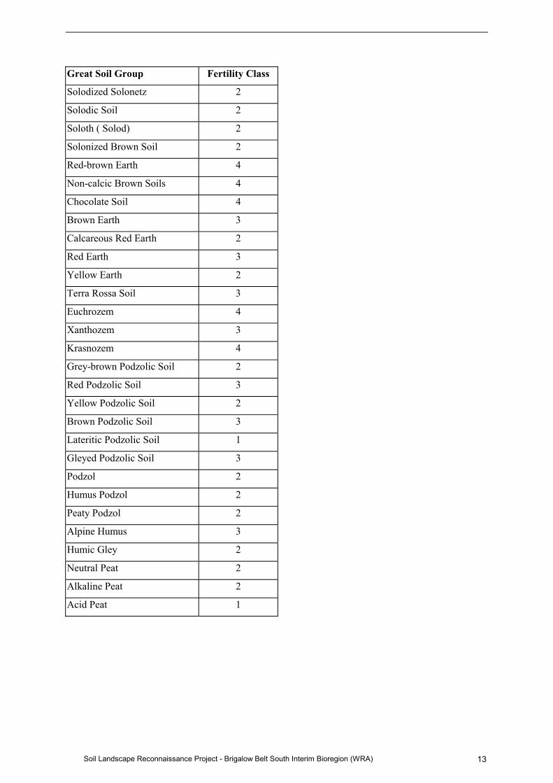
Five soil fertility classes (see Table 2) were developed, based on the Great Soils Group (GSG)classification (Stace et al. 1968), using a method outlined originally in Charman (1978) andsubsequently in Murphy et al. (2000). A class of “1” indicates a soil of very low fertility, while aclass of “5” indicates a soil with high fertility. Modified soil fertility classes were ascribed to eachGSG based on Table 2. Fertility classes were raised or lowered dependant on positive or negative soilfertility attributes that differed form the nodal soil description. For example, a facet such as a crestwith a Red Podzolic Soil has a fertility class of “3” (see Table 2), but this classification can bedowngraded to a modified fertility class of “2” if the soil is excessively stony and/or very shallow.Conversely, a soil’s modified fertility class may be upgraded if the soil has positive soil fertilityproperties, such as considerable depth, free drainage or high organic matter content in the topsoil.
Table 1: Fertility classes of Great Soil Groups
after Charman (1978)
Great Soil Group Fertility Class
Solonchak 1
Alluvial Soil 5
Lithosol 1
Calcareous Sand 1
Siliceous Sand 1
Earthy Sand 1
Grey-brown Calcareous Soil 1
Red Calcareous Soil 1
Desert Loam 1
Red and Brown Hardpan Soil 1
Grey Clay 3
Brown Clay 3
Red Clay 3
Black Earth 5
Rendzina 3
Chernozem 5
Prairie Soil 5
Wiesenboden 3
Solonetz 2
Soil Landscape Reconnaissance Project - Brigalow Belt South Interim Bioregion (WRA) 13
Great Soil Group Fertility Class
Solodized Solonetz 2
Solodic Soil 2
Soloth ( Solod) 2
Solonized Brown Soil 2
Red-brown Earth 4
Non-calcic Brown Soils 4
Chocolate Soil 4
Brown Earth 3
Calcareous Red Earth 2
Red Earth 3
Yellow Earth 2
Terra Rossa Soil 3
Euchrozem 4
Xanthozem 3
Krasnozem 4
Grey-brown Podzolic Soil 2
Red Podzolic Soil 3
Yellow Podzolic Soil 2
Brown Podzolic Soil 3
Lateritic Podzolic Soil 1
Gleyed Podzolic Soil 3
Podzol 2
Humus Podzol 2
Peaty Podzol 2
Alpine Humus 3
Humic Gley 2
Neutral Peat 2
Alkaline Peat 2
Acid Peat 1

Soil Landscape Reconnaissance Project - Brigalow Belt South Interim Bioregion (WRA)14
3.3.2 Drainage
Five drainage classes were defined based on the classes used by the SALIS Soil Data Cards(Abraham & Abraham 1992; Milford et al. 2001; and McDonald et al. 1990). They are:
1. Very poorly drained;
2. Poorly drained;
3. Imperfectly drained;
4. Moderately well-drained; and
5. Well-drained.
3.3.3 Effective rooting depth
Effective rooting depth (ERD) is an estimate of the soil and substrate available for tree roots topenetrate. It is an important factor in the calculation of Estimated Plant Available WaterholdingCapacity (EPAWC). Where the parent material has not fractured, or where an impeding layer for treeroots exists (e.g., pan or rock), then an estimate of ERD has been calculated. This is based on theaverage depth of soil and regolith that tree roots are likely to penetrate (ERD). Where the parentmaterial is fractured, tree roots will be able to penetrate both the solum and, to some extent,weathered parent material. Figure 3 shows how ERD is determined.
Figure 4: The calculation of estimated rooting depth
It should be noted that ERD can be a problematic attribute to measure in rocky soils and soils deeperthan 1.5 m. In such instances a modified estimate is provided based on the properties of the lowest
Soil Landscape Reconnaissance Project - Brigalow Belt South Interim Bioregion (WRA) 15
horizon and the probable solum depth. A maximum ERD of six metres is given as an arbitrary limit toroot penetration in deep alluvial soils. It should be noted that there are instances of many treessending roots far deeper than this to access water from aquifers.
To calculate the ERD:
Estimate the size, depth and number of fractures in the parent material and estimate an average depththat roots will be able to penetrate;Add this to the depth of the solum; andSubtract the Fragment Amount volume (see below) from the final calculation to get the effectiverooting depth.Example:
The soil depth is 1.2 m; fragment amount is 10%. The substrate is fractured, so roots will penetratethe substrate. The depth of the substrate to which the roots will penetrate is estimated to be 2.5 m, butonly 20% of the substrate volume is available (i.e., cracks, etc).
Derivation of ERD is achieved through the following formula:
ERD = soil depth + (substrate volume available to roots % x root penetration into substrate) -(fragment amount % x soil depth)
Thus:
ERD = 1.2 m + (20% x 2.5 m) - (10% x 1.2 m) = 1.58 metres
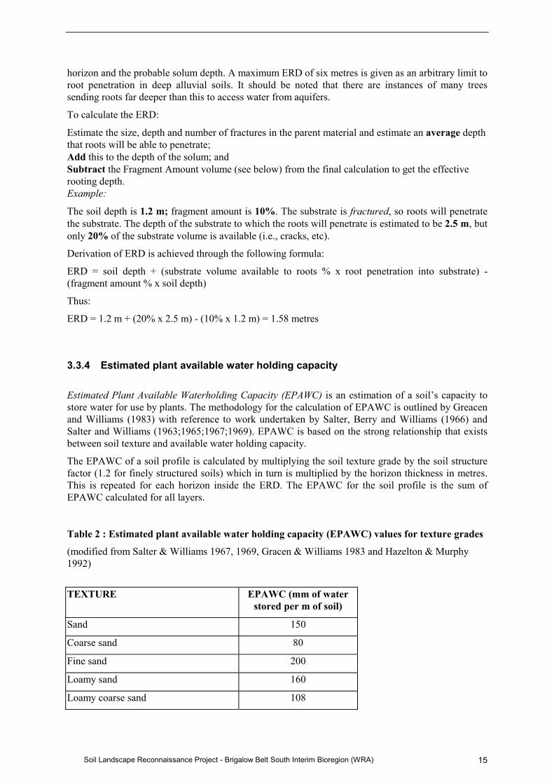
3.3.4 Estimated plant available water holding capacity
Estimated Plant Available Waterholding Capacity (EPAWC) is an estimation of a soil’s capacity tostore water for use by plants. The methodology for the calculation of EPAWC is outlined by Greacenand Williams (1983) with reference to work undertaken by Salter, Berry and Williams (1966) andSalter and Williams (1963;1965;1967;1969). EPAWC is based on the strong relationship that existsbetween soil texture and available water holding capacity.
The EPAWC of a soil profile is calculated by multiplying the soil texture grade by the soil structurefactor (1.2 for finely structured soils) which in turn is multiplied by the horizon thickness in metres.This is repeated for each horizon inside the ERD. The EPAWC for the soil profile is the sum ofEPAWC calculated for all layers.
Table 2 : Estimated plant available water holding capacity (EPAWC) values for texture grades
(modified from Salter & Williams 1967, 1969, Gracen & Williams 1983 and Hazelton & Murphy1992)
TEXTURE EPAWC (mm of waterstored per m of soil)
Sand 150
Coarse sand 80
Fine sand 200
Loamy sand 160
Loamy coarse sand 108

Soil Landscape Reconnaissance Project - Brigalow Belt South Interim Bioregion (WRA)16
TEXTURE EPAWC (mm of waterstored per m of soil)
Loamy fine sand 217
Clayey sand 150
Light clayey sand 150
Heavy clayey sand 150
Clayey coarse sand 80
Light clayey coarse sand 80
Heavy clayey coarse sand 80
Clayey fine sand 215
Light clayey fine sand 215
Heavy clayey fine sand 215
Sandy loam 180
Light sandy loam 180
Heavy sandy loam 180
Coarse sandy loam 125
Light coarse sandy loam 125
Heavy coarse sandy loam 125
Fine sandy loam 192
Light fine sandy loam 192
Heavy fine sandy loam 192
Loam 180
Loam, fine sandy 185
Silty loam 200
Light silty loam 200
Heavy silty loam 200
Sandy clay loam 150
Light sandy clay loam 150
Light - medium sandy clay loam 150
Medium sandy clay loam 150
Heavy sandy clay loam 150
Coarse sandy clay loam 140
Light coarse sandy clay loam 140
Light - medium sandy clayloam, coarse sandy
140
Medium sandy clay loam, coarse sandy 140

Soil Landscape Reconnaissance Project - Brigalow Belt South Interim Bioregion (WRA) 17
TEXTURE EPAWC (mm of waterstored per m of soil)
Heavy coarse sandy clay loam 140
Fine sandy clay loam 180
Light fine sandy clay loam 180
Heavy fine sandy clay loam 180
Clay loam 180
Light clay loam 180
Medium - heavy clay loam 180
Heavy clay loam 180
Clay loam, coarse sandy 170
Clay loam, sandy 175
Light clay loam, sandy 175
Heavy clay loam, sandy 175
Clay loam, coarse sandy 170
Light clay loam, coarse sandy 170
Heavy clay loam, coarse sandy 170
Clay loam, fine sandy 190
Light clay loam, fine sandy 190
Heavy clay loam, fine sandy 190
Silty clay loam 190
Light silty clay loam 190
Heavy silty clay loam 190
Light silty clay loam, fine sandy 195
Sandy clay 140
Sandy light clay 140
Sandy light - medium clay 140
Sandy medium clay 140
Sandy medium - heavy clay 140
Sandy heavy clay 140
Coarse sandy clay 130
Coarse sandy light clay 130
Coarse sandy light - medium clay 130
Coarse sandy medium clay 130
Coarse sandy medium - heavy clay 130

Soil Landscape Reconnaissance Project - Brigalow Belt South Interim Bioregion (WRA)18
TEXTURE EPAWC (mm of waterstored per m of soil)
Coarse sandy heavy clay 130
Fine sandy clay 150
Fine sandy light clay 150
Fine sandy light - medium clay 150
Fine sandy medium clay 150
Fine sandy medium - heavy clay 150
Fine sandy heavy clay 150
Silty clay 183
Silty light clay 183
Silty light - medium clay 183
Silty medium clay 183
Silty medium - heavy clay 183
Silty heavy clay 183
Clay 180
Light clay 180
Light - medium clay 180
Medium clay 180
Medium - heavy clay 180
Heavy clay 180
3.4 ANALYSIS
3.4.1 Geographic modelling tools
The geographic modelling environment for this study is summarised in Table 3.

Soil Landscape Reconnaissance Project - Brigalow Belt South Interim Bioregion (WRA) 19
Table 3 : The GIS software packages and their functions
Software Function Source
ESRI ArcView 3.2 Desktop vector GIS www.esri.com
Spatial Analyst Extension for ArcView 3.x enablinganalysis of raster data (grids)
www.esri.com
ER Mapper Image analysis software forconverting and manipulating gammaradiometric and satellite imagerydatasets
www.ermapper.com
Image Analyst Extension for ArcView 3.x enablinganalysis of image data
www.esri.com
S-Plus Statistical analysis package www.cmis.csiro.au/S-Plus
RPART Routines for the construction ofclassification and regression treesbased on recursive partitioning withinS-Plus (Therneau & Atkinson 1997,Venables & Ripley 1999, Atkinson &Therneau 2000)
http://lib.stat.cmu.edu/DOS/S/Swin/Rpart.zip
SLAP Extension for ArcView for terrainanalysis, coordinate transformation,derivation of erosion indices andvarious raster and vectormanipulations, developed by DrGeoff Goldrick
Soils Information SystemsUnit, DLWC
3.4.2 Soil landscape description recording
Soil landscape descriptions including assessment of soil attributes for each facet were entered into theMS Access database.
Enhanced resolution of the soil attribute information can be undertaken by linking DEMs withattributes of these facets (stored in the MS Access database) based on Compound Topographic,Elevation, Aspect and Solar Radiation Index and other factors of organisation that determinedistribution of soil types within individual soil landscape map units.

Soil Landscape Reconnaissance Project - Brigalow Belt South Interim Bioregion (WRA)20
The work program included the following steps:
4.1 PROJECT SET-UP PHASE
1. Marshall staff, initial training, obtain specialist software and equipment;
2. Literature search and entry of existing soil profiles into SALIS;
3. Establish map unit and facet strings;
Build MS Access database for soil landscape descriptions; design, test and populate;4. Soil profile attribute data entry to SALIS;
5. Assemble predictor surfaces and prepare predictor surfaces for proto-soil landscape modelling;
6. Predictor variable preparation;
7. Initial data modelling;
8. Cross-validation;
9. Smoothing of the output prediction surfaces to become maps; and
10. Initial Model Evaluation.
4.2 TRAINING AREA PHASE
1. Compilation of independent check dataset;
2. Staff briefing and work allocation;
3. Training area selection;
4. Training area pre-field preparations;
5. Training area fieldwork; and then
6. Training area digitising and database entry.
4.3 MAIN FIELDWORK AND MODELLING PHASE
1. Post-training area modelling and model iterations;
2. Modelling by province and weighting of modelling within provinces;
3. Site selection and gap analysis;

Soil Landscape Reconnaissance Project - Brigalow Belt South Interim Bioregion (WRA) 21
4. Gap analysis;
5. Flexible gap analysis;
6. Main fieldwork; and
7. Landholder communication protocols.
4.4 POST FIELDWORK PHASE
Each of the steps is detailed below:
1. Final modelling;
2. Province boundary adjustments;
3. Line work adjustments;
4. Polygon tag changes;
5. Soil profile point data gaps;
6. Soil landscape database gaps;
7. Mopping up fieldwork;
8. Linkage of soil landscape polygons and database;
9. Attribution of soil landscape spatial summary parameters;
10. Database attribution with major variables and calculation of key soil;
11. Map and database checking;
12. Design of Web products;
13. Access to information; and
14. Final report.

Soil Landscape Reconnaissance Project - Brigalow Belt South Interim Bioregion (WRA)22
The project comprised the following essential tasks:
5.1 PROJECT SET-UP PHASE
5.1.1 Marshall staff, initial training, obtain specialist software and equipment
Agreements were reached for the participation of DLWC’s Barwon Region soil surveyors and GISstaff, as well as for Dr Geoff Goldrick of DLWC’s North Coast Region. Two Technical Officers wererecruited to provide field and office support for the project. Arrangements were made for Dr Goldrickto visit soil scientists at the Centre for Land Protection Research and at CSIRO Division of Land andWater for training in the use of recursive partitioning statistical techniques. Other key staff memberswere trained to develop the MS Access database to be used for storing map unit descriptions. A highcapacity PC suitable for heavy GIS work was also ordered. This phase took four months to completedue to innumerable delays in gaining approvals.
5.1.2 Literature search and entry of existing soil profiles to SALIS
An extensive literature search was carried out. Soil profile descriptions and other data pertaining tothe project area was collected and entered into SALIS, amounting to some 1, 364 profile descriptions.
5.1.3 Establish map unit string
A map unit code string that also includes information about unmapped facets (Table 4) was devised.Use of this map unit string ensured that the soil surveyors were describing and mapping soillandscapes consistently. The string provided a shorthand way to describe a landscape for correlativepurposes, as well as to provide a unique linkage between the database and GIS coverage. The uniquelinkage was vital for populating database fields from the derived spatial surfaces.
The map unit string contains 13 alphanumeric characters and is described in Table 4. Only the lastthree or four characters of the soil landscape code were displayed on the maps� this ensured thatmap unit tags would fit comfortably within polygons.

Soil Landscape Reconnaissance Project - Brigalow Belt South Interim Bioregion (WRA) 23
Table 4: Map unit and facet string layout
ProvinceNumber(13-18)
Lithology Code(1st upper case2nd lower case)
LandformReliefModal slope(2-letterupper case)
LandformAttribute orElement(4-letter prefixlower,remainder uppercase)
SoilLandscapeCode(3 to 4-letterlower case)
Facet code(singlenumeral)
18Pilliga
VmVolcanic, mafic
RHRolling Hills
pHILHills
ahzAnt Hill
2Second largestfacet inlandscape
5.1.3.1 Provinces
To achieve the project’s aims within the restricted schedule, a number of tasks were implemented toensure orderly, on-time progress was achieved.
The BBS region was split into a number of Provinces (see Map 3), each of which corresponds to oneof the Interim Bioregion subdivisions developed by Morgan and Terry (1992). Use of thesesubdivisions allowed the BBS to be divided into broadly distinct physiographic areas, each of whichwould be allocated to an individual soil surveyor. The provinces are identified by unique numbers asfollows:
13 = Northern Outwash
14 = Northern Basalts
15 = Pilliga Outwash
16 = Liverpool Plains
17 = Pilliga
18 = Liverpool Ranges
19 = Talbragar
Province numbers less than 13 have already been used by previous projects.
The province boundaries were subsequently subdivided and adjusted using existing geology mapsand the work of Hesse (2000) (see Map 4).
Some provinces were further subdivided to facilitate modelling as the survey was nearing completion.These changes did not require any further alterations to the string.
5.1.3.2 Lithology code
Lithology (as a substitute for soil parent material) has proven to be useful in mapping the soils of theUpper North-east and Southern CRA Areas. Lithology in these areas simplified a plethora ofgeological mapping units of slightly different ages but fundamentally the same geology and soils. Thelithology code used was based on Gray and Murphy (1999) and is listed in the table below. However,
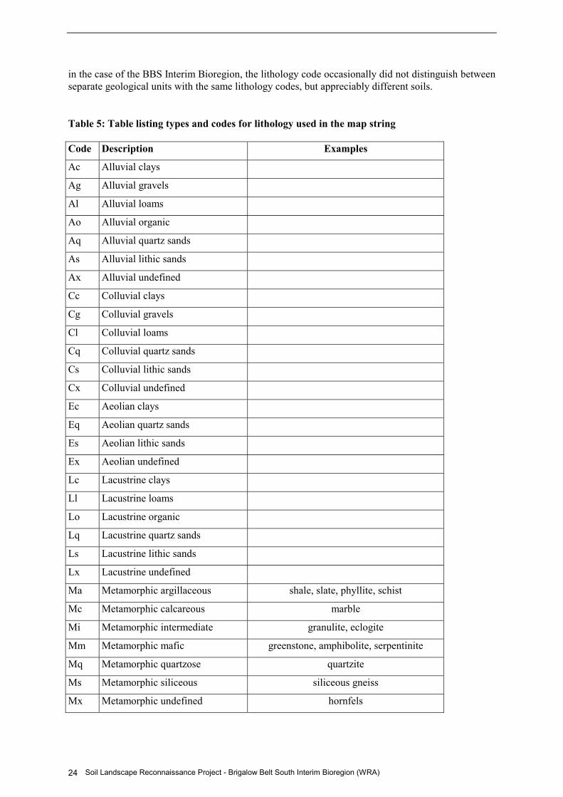
Soil Landscape Reconnaissance Project - Brigalow Belt South Interim Bioregion (WRA)24
in the case of the BBS Interim Bioregion, the lithology code occasionally did not distinguish betweenseparate geological units with the same lithology codes, but appreciably different soils.
Table 5: Table listing types and codes for lithology used in the map string
Code Description Examples
Ac Alluvial clays
Ag Alluvial gravels
Al Alluvial loams
Ao Alluvial organic
Aq Alluvial quartz sands
As Alluvial lithic sands
Ax Alluvial undefined
Cc Colluvial clays
Cg Colluvial gravels
Cl Colluvial loams
Cq Colluvial quartz sands
Cs Colluvial lithic sands
Cx Colluvial undefined
Ec Aeolian clays
Eq Aeolian quartz sands
Es Aeolian lithic sands
Ex Aeolian undefined
Lc Lacustrine clays
Ll Lacustrine loams
Lo Lacustrine organic
Lq Lacustrine quartz sands
Ls Lacustrine lithic sands
Lx Lacustrine undefined
Ma Metamorphic argillaceous shale, slate, phyllite, schist
Mc Metamorphic calcareous marble
Mi Metamorphic intermediate granulite, eclogite
Mm Metamorphic mafic greenstone, amphibolite, serpentinite
Mq Metamorphic quartzose quartzite
Ms Metamorphic siliceous siliceous gneiss
Mx Metamorphic undefined hornfels

Soil Landscape Reconnaissance Project - Brigalow Belt South Interim Bioregion (WRA) 25
Code Description Examples
Oc Marine clays
Og Marine gravels
Ol Marine loams
Oo Marine organic
Oq Marine quartz sands
Os Marine lithic sands
Ox Marine undefined
Pi Plutonic intermediate granodiorite, syenite, monzonite, diorite
Pm Plutonic mafic gabbro, dolerite, wherlite
Ps Plutonic siliceous granite, adamellite, quartz porphyry
Pu Plutonic ultramafic dunite, peridotite
Px Plutonic undefined porphyry
Sa Sedimentary argillaceous mudstone, claystone
Sc Sedimentary calcareous limestone, dolomite
Sf Sedimentary ferromanganiferous laterite, ferricrete, bauxite
Si Sedimentary intermediate greywacke
Sl Sedimentary lithic (coarse) lithic sandstone and conglomerate
So Sedimentary organic coal, peat
Sq Sedimentary quartzose chert, jasper, silcrete
Ss Sedimentary siliceous quartz sandstone, quartz siltstone
Sx Sedimentary undefined turbidite, clastics
Ux Unconsolidated undefined
Vi Volcanic intermediate dacite, trachyte, andesite, intermediate tuff
Vm Volcanic mafic basalt, picrite, mafic tuff
Vs Volcanic siliceous rhyolite, dellenite, siliceous tuff
Vx Volcanic undefined tuff, pyroclastic, pumice, ash
Xx Undefined

Soil Landscape Reconnaissance Project - Brigalow Belt South Interim Bioregion (WRA)26
5.1.3.3 Modal slope code
The two-letter modal slope codes used in this project are based on those of McDonald et al. (1990).Examples include UR - undulating rises; SH - steep hills; and PM - precipitous mountains.
5.1.3.4 Landform pattern or element code
These three-letter codes describe unique landform patterns or elements, as described in McDonald etal. (1990). These were used to determine similarities between map units described by different soilsurveyors. Attributes of landform patterns cover such things as HIL - hills, SAN - sandplain, ALP-alluvial plain and DUN - dunefield. Where significant, landform element codes were also used—e.g.,HCR - hillcrest, HSL - hillslope, FOO - footslope, BRI - beach ridge and TAL - talus, etc. Prefixes"p" and "e" identify landform patterns and elements respectively.
5.1.3.5 Soil landscape code
Soil landscapes were used to delineate areas of different soils by using distinguishing landscapefeatures (especially those important to vegetation modelling). Each soil landscape was given a three-letter code. Three-letter codes allowed the inclusion of published two-letter soil landscapes codes(e.g., ki from the local geographic name Kindamindi) and their variants with three-letter codes (e.g.,kia) to be given the same length character code. To achieve a consistent three-letter code systemacross all mapped units, normal soil landscapes were allocated an extra letter (using a descendingseries starting with z), which also allowed different soil landscapes from different areas with the sametwo-letter code to be distinguished (e.g., ki would become kiz).
Later, a four-letter code was added so that the originating soil surveyor could be linked with themodelled output and the map unit description.
A soil landscape variant usually has a different property than the parent soil landscape, e.g.,shallower soils, but generally all other soil landscape features are similar. The letter a is used toidentify the first soil landscape variant of the parent soil landscape. Any subsequent variants weregiven alphabetically ascending postscripts (e.g., b, c, d, etc). Although not mutually exclusive, thecode was linked in the database to the long map unit string code, which was unique and ensures thateach soil landscape is linked to appropriate data in the database.
5.1.3.6 Facet code
As mentioned earlier, facets are a way of dividing a landscape into discrete sub-units that eachcontains a distinct soil type or suite of soil types at a scale too fine to be depicted on 1:100 000-scalemaps. This methodology has been used previously in generating soil landscapes in the BBS area—e.g., the soil landscape modelling by Banks (1998) uses facets and was included during modelling.
The soil surveyor nominates the percentage area of the soil landscape covered by each facet. Thepercentage of the parent soil landscape does not reflect any modelled probability of occurrence or amodelled spatial percentage.
Modellers can map facets at a finer scale by using collateral data sets like DEMs because each facetis given a description of the main landform, lithological, climatic or soil factor used to delineate itfrom other facets. This is known as a Factor of Organisational Grouping (FOG) value (see Table 7).

Soil Landscape Reconnaissance Project - Brigalow Belt South Interim Bioregion (WRA) 27
For each facet in any soil landscape, an identifier is used. Facets are generally numbered inaccordance with the area that they occupy, with the number 1 being allocated to the most extensivefacet, 2 allocated to the next most extensive facet, and so on.
Example of a long string map unit code. The map unit code 18VmRHpHILahz(2) is used todefine a map unit on the Liverpool Ranges province with volcanic mafic lithology, a rolling hillmodal slope class, a hills landform pattern, an ahz soil landscape code and the (2) second largestfacet. A record at facet level in the database shows that this facet occurs across about 10% of the soillandscape, its location is determined by elevation and that the elevation range is the highest in thelandscape. This long string code is unique in NSW for all soil landscape map units.
5.1.4 Build MS Access database for soil landscape descriptions
An MS Access database similar to the database used for the Southern CRA soils project and othersoils mapping projects in western NSW was developed and populated for this project.
The central database was used to set-up, correlate, store and keep track of the soil landscapeinformation collected by the soil surveyors. A user-friendly data entry screen with pull down buttonsfor many attributes ensured that consistent information was entered, reducing the likelihood of errorsin the dataset. The data entry screen is linked to separate soil landscape and facet tables that allowready export and linking with other databases and GIS.
Each soil surveyor was given a copy of the database, which was to be filled in following fieldworkand its contents added to the main central database. To ensure version control and to prevent anyconfusion between map unit description updates, a file-naming protocol was implemented.Centralising the database allowed the data to be readily verified and controlled at a single location.Table 6 provides a list of the information recorded in the database for each soil landscape.
Table 6: Soil and landscape properties recorded for each soil landscape unit in the MS Accessdatabase
Database attribute Description
Soil landscape name The name of the soil landscape
Soil landscape code Three to four-letter soil landscape string that occurs on the maps. It is notunique and the code can occur on numerous mapsheets, but is linked to thesoil landscape string and secondary mapsheet units that identifies thecorrect dataset in the database.
Protosoil-landscapecode
Original map unit code, derived from model.
Soil landscapestring
13-character string contains code information for province, lithology,modal slope code, landform pattern or element and soil landscape/soillandscape variant code. It is unique in the database.
Completed by Identifies the person responsible for the entry of the soil landscape into thedatabase.
Date completed Identifies the date the soil landscape was entered into the database.
Mapsheet number Topographic 1:100 000 mapsheet number, e.g., 8838.
Process group Soil landscape geomorphologic groups. Examples include residual,erosional, alluvial and aeolian.

Soil Landscape Reconnaissance Project - Brigalow Belt South Interim Bioregion (WRA)28
Database attribute Description
Province number One of six province codes is entered. Makes up part of landscape string.
Lithology code DLWC lithology codes.
Modal slope code Modal slope code entered.
Landform patternor element code
Landform pattern - element class.
Included soillandscapedescription
Lists soil landscapes included within the soil landscape being described.
Variant description Variant description entered
Geology code The geology code.
Minimum andMaximum elevation
Minimum and maximum elevation (in metres) of the soil landscape.
Minimum andMaximum slope
Minimum and maximum slope for the soil landscape.
Local relief Relief of the soil landscape.
Rock outcrop % of rock outcrop in soil landscape.
Dominant lithology Dominant CSIRO lithology code.
Sub-dominantlithology code
Sub-dominant CSIRO lithology code.
Dominantstructuralformation class forvegetation
Dominant original structural class for vegetation.
Sub-dominantstructuralformation class forvegetation
Sub-dominant original structural class for vegetation.
Dominant land use Up to three dominant land uses.
Sub-dominant landuse
Up to three sub-dominant land uses.
Confidence rankingfor soil landscape
A confidence ranking (1 - 9) that the soil landscape unit is applicable.
Count of totalnumber of facets
A total count of the number of facet records within the selected soillandscape record.
Landscapelimitations
Major soil and landscape limitations that are likely to be present and poserestrictions to urban and rural activities. Limitations are described as eitherlocalised or widespread. Limitations include steep slopes, mass movementhazard, rockfall hazard, flood hazard, waterlogging, permanently highwatertables, seasonal waterlogging, water and wind erosion hazard, highrun-on, mine subsidence district, shallow soil, non-cohesive soil, surface

Soil Landscape Reconnaissance Project - Brigalow Belt South Interim Bioregion (WRA) 29
Database attribute Description
movement potential, rock outcrop, high foundation hazard, groundwaterpollution hazard, wave erosion hazard, gully and sheet erosion risk,complex soils, periodically frozen soils, potential saline aquifer rechargezone, saline discharge zone, salinity hazard, seepage scalds and woodyweeds.
Notes andcomments
Notes on the soil landscape.
The database also contains data collected and applicable at the facet level. The pertinent fields aredetailed in Table 7. The table contains fields that relate to Factor of Organisational Groupings(FOGs). FOGs are the external attributes by which a facet can be delineated using GIS to map likelyfacets at intense scales of 1:25,000. The characteristics of the dominant facet can be used as ananalog to the behaviour of its parent soil landscape, or alternatively weighted averages can be used toshow the gross distribution of soil depths, fertility and plant available water capacities across thelandscape.
Table 7 : Facet properties recorded for each soil landscape unit in the MS Access database
Database attribute Description
Facet code 14-character string code (the soil landscape 13-character string with an extranumber added as a postscript and starting with the number 1 and increasingconsecutively for each new soil sub-landscape present), e.g., 18VmRHpHILahz(1) is the first soil sub-landscape in the map unit18VmRHpHILahz landscape. Every soil landscape has at least 1 andgenerally � 4 soil sub-landscapes.
Additional facetnotes
Additional facet notes.
% of soil landscape the average % of area which the facet covers.
Nature of profile The type of profile used. Includes published type profile, field observation,CRA type profile and other information.
SALIS type profileand associatedSALIS surveynumber
SALIS profile number and associated SALIS survey number.
GSG and itsassociated fertility
Great Soil Group classification and associated fertility.
Soil depth The mean estimated soil depth is entered for each facet.
Mean estimatedeffective rootingdepth
Mean estimated effective rooting depth, i.e., the volume of soil/voids insubstrate that are accessible by tree roots is provided.
Mean modifiedfertility
Mean modified fertility class for each soil sub-landscape if given .
Estimated plantavailable
EPAWC is provided for each soil sub-landscape.

Soil Landscape Reconnaissance Project - Brigalow Belt South Interim Bioregion (WRA)30
waterholdingcapacity (EPAWC)
Mean drainage Mean drainage class of the soil sub-landscape.
Soil regolith class Soil regolith stability classification after Murphy, Fogarty and Ryan (1998)classifies the stability of a soil for forestry uses into four classes. Class 1 isstable coherent soils with low sediment delivery potential to streams. Class2 is non-coherent sandy soils with low sediment delivery. Class 3 iscoherent soils with high sediment delivery. Class 4 is non-coherent soilswith high sediment delivery potential.
FOG-landformelement
Identifies the landform element attributes that were used to subdivide thesoil landscape into facets, e.g., plain, hillslope, fan, ox-bow.
FOG-sitemorphology
Identifies the site morphology attributes that were used to subdivide the soillandscape into facets, e.g., upper slope, midslope, open-depression.
FOG-landformpattern
Identifies the landform pattern attributes that were used to subdivide the soillandscape into facets, e.g., alluvial plain, terrace, plateau.
FOG-relativeelevation
Identifies the relative elevation attributes that were used to subdivide thesoil landscape into facets, e.g., lowest, middle, highest.
FOG-site exposure Identifies the site exposure attributes that were used to subdivide the soillandscape into facets, e.g., sheltered, moderately exposed, highly exposed.
FOG-substratelithology
Identifies the substrate lithology attributes that were used to subdivide thesoil landscape into facets, e.g., alluvial, basalt, sand, granite.
FOG-remotesensing pattern
Identifies the remote sensing attributes that were used to subdivide the soillandscape into facets, e.g., radiometric signature like high K.
FOG-other Identifies the other attributes that were used to subdivide the soil landscapeinto facets, e.g., soil type.
The database was populated for all existing map units in the study area and tested against apreliminary map. A map unit string was used to link the database to the GIS map product.
There are over 500 different soil landscape map units and over 1,100 facets in the final database.
5.1.5 Build WRA Soil Data Card for SALIS with appropriate fields for western soilconditions
Soil conditions in the western part of NSW differ considerably from prevailing conditions in higherrainfall areas of the state. A two-page Western Regional Assessment Soil Data Card was designedwith input from experienced soil surveyors that contained fields of value to the survey:
� Reason for profile selection: e.g., random; bulked sample; opportunistic; curiosity/unusual soil;boundary checking; pre-planned; transect/catena; grid; type profile. Type profiles are consideredto be representative of the soil within a facet.
� Segregation types: carbonate and gypsum added to the existing set.
� Salinity test results.
� Crumb test (for dispersion and slaking).
� Testing for pH as alkalinity and acidity can vary throughout the area.

Soil Landscape Reconnaissance Project - Brigalow Belt South Interim Bioregion (WRA) 31
5,000 of these cards were printed. Delays were experienced in having SALIS programmed to acceptthe new fields on the cards because of other corporate priorities.
Many casual observations were also made and recorded on field sheets and in notebooks. Table 8shows the field attributes recorded at each site on the WRA observation cards.
Table 8: Site and soil attributes recorded on WRA Soil Data Cards
Parameter field Attribute
Landform Site morphology
Landform pattern
Site disturbance
Land use (site and general area)
Erosion type, its severity and present condition
Topography Slope gradient
Aspect
Microrelief
Lithology Solum parent material
Substrate
Geology map code
Soil A-horizon
Solum
Depth to impeding layer
Estimated rooting depth
Layer colour
Layer soil texture
Layer soil structure
Layer grade of structure
Fragment amount
Segregation type and amount
Soil Ph
Crumb, AgNO3, HCl and field dilatancy tests
Erosion hazard
Surface salinity
Layer permeability
Surface condition (wet and dry)
Australian Soil Classification
Great Soil Group Classification
Soil map code
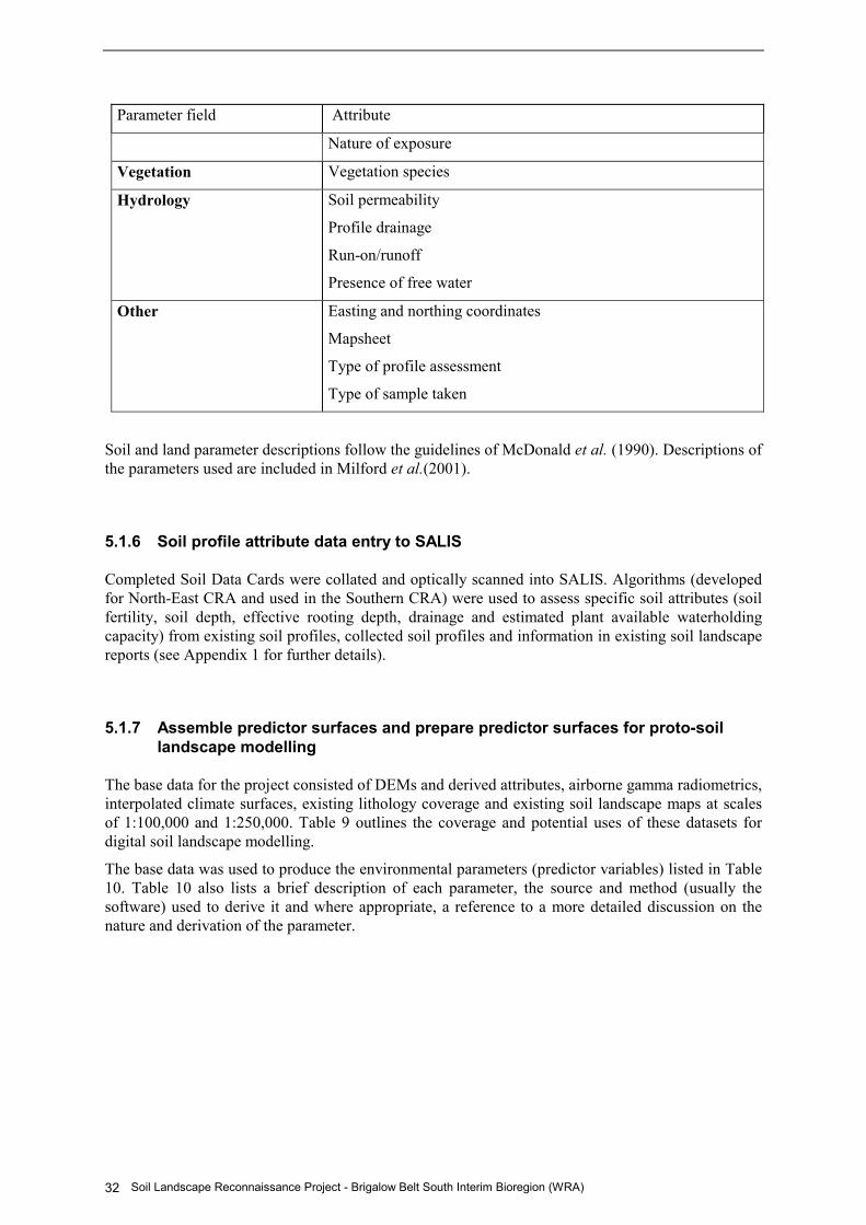
Soil Landscape Reconnaissance Project - Brigalow Belt South Interim Bioregion (WRA)32
Parameter field Attribute
Nature of exposure
Vegetation Vegetation species
Hydrology Soil permeability
Profile drainage
Run-on/runoff
Presence of free water
Other Easting and northing coordinates
Mapsheet
Type of profile assessment
Type of sample taken
Soil and land parameter descriptions follow the guidelines of McDonald et al. (1990). Descriptions ofthe parameters used are included in Milford et al.(2001).
5.1.6 Soil profile attribute data entry to SALIS
Completed Soil Data Cards were collated and optically scanned into SALIS. Algorithms (developedfor North-East CRA and used in the Southern CRA) were used to assess specific soil attributes (soilfertility, soil depth, effective rooting depth, drainage and estimated plant available waterholdingcapacity) from existing soil profiles, collected soil profiles and information in existing soil landscapereports (see Appendix 1 for further details).
5.1.7 Assemble predictor surfaces and prepare predictor surfaces for proto-soillandscape modelling
The base data for the project consisted of DEMs and derived attributes, airborne gamma radiometrics,interpolated climate surfaces, existing lithology coverage and existing soil landscape maps at scalesof 1:100,000 and 1:250,000. Table 9 outlines the coverage and potential uses of these datasets fordigital soil landscape modelling.
The base data was used to produce the environmental parameters (predictor variables) listed in Table10. Table 10 also lists a brief description of each parameter, the source and method (usually thesoftware) used to derive it and where appropriate, a reference to a more detailed discussion on thenature and derivation of the parameter.

Soil Landscape Reconnaissance Project - Brigalow Belt South Interim Bioregion (WRA) 33
Table 9: Base datasets used in the BBS study and their potential uses
Dataset (coverage) Uses References
Gamma Radiometrics
(Missing from north of studyarea and fromWarrumbungles)
Signal taken from dry soils todepths of up to 50 cm.Discrimination of soil parentmaterials and interpretation oflandforming processes,interpretation of soil depthand veneers of aeolianmaterials
Wilford et al. 1997; Pickupand Marks 2000.
Digital Elevation Models
(9 sec DEM complete; 25 mDEM complete except north-western portion of Narrabri1:250,000 sheet)
Derivation of terrainattributes as predictors of soillandscape class; importantpredictor for drainage anddepositional and erosionalprocesses
Moore et al. 1993; Wilsonand Gallant 1996; Wilson andGallant 2000.
Interpolated ClimateSurfaces (see Table 10)
(Complete but accuracy ofinterpolations betweensurfaces is dependant onsparse datasets)
Climate as a predictor ofbiological activity, soilmoisture regime and hencesoil type; fire regimeinfluenced by climateinfluences soil parameters
Hutchinson 1991; McKenzieand Ryan 1999.
Lithology
(Complete but composed oftiles of maps of differentstyles and purposes - notcontinuous)
Major determinant of soilmineralogy
Gray and Murphy 1999;Paton et al. 1995.
Soil Landscapes and otherSoil Maps
(Limited coverage, mostly insouth. Mapped at 1:100,000and 1:250,000 scales withedge mismatches betweenmapping scales and differentunit names - not continuous.)
Tested model of soildistribution in the landscape
Banks 1998.
Soil Profile DescriptionPoints
(Limited, mostly distributedthroughout areas of previoussoil mapping)
Point locations of soil types

Soil Landscape Reconnaissance Project - Brigalow Belt South Interim Bioregion (WRA)34
The parameters and predictor variables obtained from these datasets were used to derive thefollowing variables for use in the model.
Table 10: The environmental parameters (predictor variables) used for modelling andprediction of soil landscapes in the BBS
Parameter Description (units) Source/Method Reference
Elevation height above sea level(m)
DEM
Slope slope gradient (�) DEM + ArcView +SLAP
Wilson et al. 2000
Compoundtopographic index(CTI)
measure oftopographic controlon soil moisturebased on slope anddownslope flowaccumulation
DEM + ArcView +SLAP
Wilson et al. 2000
Profile curvature measure of thedownslope rate ofchange(slope/gradient)
DEM + ArcView +SLAP
Wilson et al. 2000
Tangentialcurvature
measure oftopographicconvergence anddivergence
DEM + ArcView +SLAP
Wilson et al. 2000
Relative elevationindex (REI)
local (300m radius)measure of positionin the landscape
DEM + ArcView +SLAP
Goldrick (this study)
Temperature (meanannual)
�C DEM + ANUCLIM Houlder et al. 1999
Precipitation (meanannual)
Mm DEM + ANUCLIM Houlder et al. 1999
Moisture index(mean annual)
measure of thebalance betweenprecipitation andevaporation
DEM + ANUCLIM Houlder et al. 1999
Moisture index(coefficient ofvariation)
measure of theseasonality of themoisture index
DEM + ANUCLIM DEM + ANUCLIM
Radiation index relative index of thetotal annual amountof radiation modifiedfor slope and aspect
DEM + ANUCLIM +ArcView + SLAP
Potassium gammaray count
Wilford et al. 1997

Soil Landscape Reconnaissance Project - Brigalow Belt South Interim Bioregion (WRA) 35
Parameter Description (units) Source/Method Reference
Thorium gammaray count
Wilford et al. 1997
Uranium gammaray count
Wilford et al. 1997
Parent materiallithology
reclassification ofgeological units
DMR Geology Gray et al. 1999
5.1.8 Predictor variable preparation
All base data and predictor variables were converted to ArcView grids for use in Spatial Analyst.Many datasets were not available in this form. Also, many datasets needed to be joined into singlethemes as they consisted of several tiles. Grids were then reprojected to the BBS-WRA standard(Australian Map Grid Zone 55 with a central meridian located at 147 Transverse Mercator AustralianSpheroid scale factor 0.9996, False Easting 500000 and False Northing 10000000). These routineswere performed using SLAP. The resultant surfaces consisted of grids with 25 m cells.
Digital climate drapes for all available climatic variables were prepared using the ESOCLIM 5.0software. These were modified according to the effect of terrain as derived from DEMs.
5.1.9 Initial data modelling
To “train” the soil landscape model, 25,000 sample points were randomly generated for the areacovered by existing 1:100 000 scale soil landscape data (Figure 5).

Soil Landscape Reconnaissance Project - Brigalow Belt South Interim Bioregion (WRA)36
Figure 5: Extent of existing 1:100,000 (yellow) and 1:250,000 (blue) soil landscape mapping inthe BBS
The 1:250 000 scale soil landscape data was excluded for this preliminary analysis due toincompatibilities in the soil landscape classes, but these are being resolved for future analyses. Use of25,000 sample points is arguably excessive because if meaningful relationships do exist between soillandscapes and environmental parameters, they should become evident at much lower samplingdensities. However, it was considered preferable to over-sample the training data and then reduce treecomplexity (by the methods described below), rather than run the risk of under-sampling and missingimportant relationships.
A training data matrix was constructed from the sample points with soil landscape class as thedependent (y) variable and the environmental variables in Table 10 as the predictor (x) variables.Because radiometric coverage was incomplete, two training data matrices were used, one includingradiometric data but omitting lithology, the other including lithology but omitting radiometric data.
These two datasets were analysed using RPART to create a classification tree (Figure 6). Aclassification tree is a method of hierarchically splitting a dataset into increasingly homogenoussubsets. The criterion for each split is to minimise some measure of the impurity of the resultantclasses, in this case the Gini index (see Therneau & Atkinson 1997; and Venables & Ripley 1999 fordetails).

Soil Landscape Reconnaissance Project - Brigalow Belt South Interim Bioregion (WRA) 37
Figure 6: A partial classification tree (upper nodes and branches) from the RPART analyses ofthe training data including radiometrics for the BBS indicating the decision criteria
Note: the first modelled and pruned tree has 451 nodes and is too complex to illustrate.
Two important controls on RPART are “minsplit” and “cp”. The former determines the minimumnumber of observations in a node for which the routine will try to compute a split. The latter is ameasure of tree complexity (Venables & Ripley 1999) with values ranging from 0 to 1 and lowervalues indicating greater complexity. For the BBS datasets, “cp” was initially set to 0.000001 and“minsplit” set to 2 to allow a very complex tree to be generated.
5.1.10 Cross-validation
The classification trees were constructed with 10-fold cross-validation. Cross-validation involvessplitting the training data into roughly equal-sized subsets and growing the tree on all but one of thesesubsets, and testing it with the unused portion of the dataset (Venables & Ripley 1999). In this case,the training data was split into 10 subsets, then 9 were used to grow the tree and the tenth used to testit. This was repeated 10 times (for each combination of subsets) and the results averaged to producethe final tree.

Soil Landscape Reconnaissance Project - Brigalow Belt South Interim Bioregion (WRA)38
5.1.10.1 Tree ‘pruning’ to reduce complexity
A tree with few “leaves” (terminal nodes) is likely to “under fit” the data— i.e., it is unlikely toadequately reflect the complexity of the relationship between the predictor variables and thedependent variable. On the other hand, a tree with very many leaves may “over fit” the data— i.e., itreflects noise within the data rather than meaningful relationships. Cross-validation provides ameasure for “pruning” the tree in order to reduce its complexity. As the size of a tree increases, thecross-validation error tends to decrease until it reaches a minimum. After this point, the cross-validation error may remain steady or even increase with increasing tree size (Figure 7).
Figure 7: The relationship between tree complexity and cross-validation error for theclassification trees of the BBS based on radiometrics
In other words, beyond this minimum increasing, the size of the tree does not increase theinformation about the relationship between the predictor and dependent variables. So this minimumprovides an objective basis for tree pruning. Venables and Ripley (1999) suggest applying the 1-SErule— i.e., to select the smallest tree with a cross-validation error within one standard error of theminimum cross-validation error. For example, the unpruned tree for the BBS training matrix withradiometrics had 3,794 leaves, but a plot of tree size versus cross-validation error indicates that if the1-SE rule is applied, the tree may be pruned to 451 leaves with no meaningful loss of information(Figure 7). At this level of complexity (cp = 0.0002), the misclassification rate is about 26 per cent.
For the training matrix with lithology, the initial tree had 6,958 leaves, but this was pruned to 895leaves with cp = 0.0001 and a resultant misclassification rate of 28 per cent. It is important to re-emphasise that a "perfect" fit could be achieved by setting cp = 0, but this would merely result in anexceedingly complex tree that reflects noise (inherent in any natural database), such as soillandscapes. The appropriate pruning allows description of meaningful relationships between thepredictor variables and the soil landscapes.
The pruned trees were then translated into an Avenue script for generating a grid of predicted soillandscape classes. The two grids were combined such that the values from the radiometric tree tookprecedence over values from the lithology tree.

Soil Landscape Reconnaissance Project - Brigalow Belt South Interim Bioregion (WRA) 39
5.1.11 Smoothing of the output prediction surfaces to become maps
The combined grid was simplified by passing a modal filter over the grid and then removing regionsless than 80 cells in size� about 20 ha, the minimum mapping area specified by Reid (1988). In theoutwash areas of subdued topography and large-scale fan influences, the minimum mapping areaswere increased to 40 ha (Reid 1988) by absorbing them into adjacent regions. The initial grid ofpredicted soil landscape class for the whole BBS is shown in Figure 8 on the following page.
5.1.12 Initial model evaluation
The grid model of the Curlewis 1:100,000 soil landscapes was smoothed to minimum mapping areaof 20 ha (i.e., eighty 25 m x 25 m cells) and compared with Curlewis original soil landscapes. Themodel compared favourably with the original mapping (see Figure 8b).
The model was also compared with other portions of the BBS area against local knowledge. Themodel outputs did not predict well where other landscape and soil-forming processes becomedominant and where the predictor variables are not sufficiently sensitive.
It was decided that a number of small training areas would be established to guide the model in areasthat did not have representative soil mapping.
5.2 TRAINING AREA PHASE
5.2.1 Compilation of independent checking dataset
An independent soil data checking set of around 130 locations for the study area was considered to besufficient, being around 10 per cent of the dataset expected to be collected as a result of fieldworkfrom the project (Reid 1988). The points sampled were confined to areas without existing (andchecked) soil landscapes as these had already been thoroughly field checked.
The check sampling points were mostly restricted to public roads and other accessible areas.
Sampling locations were initially stratified according to broad geological types and landform patternsbeing evenly distributed across 1:100 000 map sheets. It was later decided to complete theindependent sampling set at the end of the main mapping phase at locations where both flora andfauna had been sampled.
The soil profile information from the independent check dataset was not used during the mainmapping phase.
5.2.2 Staff briefing and work allocation
A meeting was held in May in Gunnedah where the project background, methodology, requirementsand database were discussed. File name protocols and database version control rules were discussed.Work areas were allocated and training areas were selected.
Figure 8: Grid of predicted soil landscapes as initially modelled for the south-eastern portion ofthe BBS (a) and detail of a section with overlay of the training data line work (b)

Soil Landscape Reconnaissance Project - Brigalow Belt South Interim Bioregion (WRA)40
(a)
(b)
The above analysis is based on soil landscape mapping on the Curlewis 1:100 000 map sheet (Banks1995). Blocks of colour represent the modelled soil landscape outputs, whereas the black linesrepresent the original soil landscape mapping.

Soil Landscape Reconnaissance Project - Brigalow Belt South Interim Bioregion (WRA) 41
5.2.3 Training area selection
To overcome the problem of existing soil landscapes representing the rest of the study area,additional mapping using air photo interpretation and field observation for several small areasscattered throughout the BBS was required. The aim was to create training datasets with a broadcoverage of various environmental conditions of the BBS and then interpolate between these trainingdatasets, rather than extrapolate models outwards from a single training set.
Nine training areas were selected on the basis of geomorphic and radiometric patterning in datasparse areas. Each training area was located to maximise the greatest amount of topographic andparent material variation in a reasonably small and accessible area. Map 2 shows the locations of thetraining areas.
1:100 000-scale soil landscape mapping already in progress was accelerated. In particular, line workwas completed and scanned to ensure that these preliminary maps could be provided and also usedfor training. It was realised that the 1:250 000 soil landscape mapping would confound the modelbecause of the conflicting scale and potential overlap between the two scales of mapping inintermediate areas. Consequently the 1:250 000 scale mapping was not used for training until later inthe project.
5.2.4 Training area pre-field preparations
Literature review and reconnaissance of each training area was undertaken. Base maps were preparedshowing context information, navigational data and, where possible, radiometrics and topographicfeatures. Each area was examined using radiometrics and air photos in stereoscopic pairs. Preliminarysoil landscapes were delineated.
A copy of the database populated with existing soil landscapes was provided to each soil surveyor.To keep the model as simple as possible and, more importantly, to prevent map unit decision conflictsin the model, instructions were issued to ensure that no new units were to be produced that duplicatedprevious mapping.
5.2.5 Training area fieldwork
The soils and associated physiographic information for each facet within each soil landscape in eachtraining area was observed and recorded on WRA Soil Data Cards.
5.2.6 Training area digitising and database entry
Training area field sheets were traced and despatched for scanning. The resulting digital soil mapswere edited and despatched for use in the model.
Complete descriptions for all soil landscapes were entered into the MS Access database. Somecommunication problems and iterative changes to training area line work delayed this process.

Soil Landscape Reconnaissance Project - Brigalow Belt South Interim Bioregion (WRA)42
5.3 MAIN FIELDWORK AND MODELLING PHASE
Expert knowledge can be incorporated into the tree-based soil landscape models at several stages,including the initial choice and derivation of predictor variables, pre-stratification, and assessmentand modification of the decision rules produced by the model.
The success of the model was primarily dependent on the choice of appropriate predictor variablesand the high-quality datasets that describe them. The range of possible predictor variables is verylarge, and expert knowledge was required to determine which of these would be the better predictorsof soil landscape class in particular areas.
Figure 9: Detail of area around Narrabri illustrating the usefulness of the REI for identifyinglevees (red) and depressions (blue)
It was also possible to manipulate base environmental data to develop new predictor variables. Forexample, in the broad alluvial plains of the BBS it is known that the soils of elevated areas such aslevees and dunes are different from the soils of the surrounding plain (Banks, R. 2002, pers. comm).However, the difference in elevation that defines such features is often subtle and hard to identifyreliably from raw elevation data. This association led to the development of the relative elevationindex (REI), which was designed specifically to identify such features. REI values were found tocorrelate well with the existence of levees and depressions (Banks, R. 2002, pers. comm.; Figure 9).
Another example of the use of expert knowledge to manipulate base datasets is the reclassification ofgeology into lithological parent material. This is important because geological classes may bedifferentiated on a variety of characteristics unrelated to their role as soil parent material.Reclassification of the geological database allowed the number of classes to be reduced from 409 to24 in a way that emphasised this role. It was later found, in the West Pilliga, that lithology wasinsufficient to discriminate between some soils. As a result of field checking and soil surveyorfeedback, the model was altered to include geology tags in these areas.

Soil Landscape Reconnaissance Project - Brigalow Belt South Interim Bioregion (WRA) 43
5.3.1 Post-training area modelling and model iterations
The model was run using the training datasets. Because of the relative size of the new trainingdatasets compared to the original soil landscape trained areas, the model remained dominated by theweighting of parameters in the Liverpool Plains and Liverpool Ranges. For example, climateparameters that were important soil landscape discriminators in the Liverpool Ranges were notappropriate for this purpose in the topographically subdued Pilliga outwash.
5.3.2 Modelling by province and weighting of modelling within provinces
The decision was made to use the provinces of Morgan and Terry (1992) as separate modelling areas.The model was run separately for each area and adjustments made on the advice of soil surveyors.Soil surveyors spent at least one day providing input to their modelled provinces. A brief synopsis ofeach province is listed below.
5.3.2.1 Liverpool Ranges
The model worked well here due to excellent training areas, a single geological province (basalt andassociated lithologies) and strong relief and terrain, which allowed DEM parameters to be usedconsistently.
5.3.2.2 Liverpool Plains
The southern portion modelled well initially, but prediction was poor in the northern part. Climateand elevation parameters were reduced in importance, but the model still failed to perform. Draft soillandscape mapping from the Baan Baa and Boggabri 1:100 000 map sheets was then scanned,checked and used directly.
This left a remaining small section of <500 km2 in the north to be modelled. However, the model didnot perform well on much of this area due to the strong influence of fan soil landscapes (originatingin the Nandewar Ranges Interim Bioregion to the east of the BBS, for which no training areas wereavailable). Further fieldwork was undertaken to describe these soil landscapes.
In summary, the Liverpool Plains was judged to be satisfactory, being based on soil landscape linework, except for a small portion in the extreme north-east.
5.3.2.3 Talbragar Valley
This province had been entirely mapped with 1:250 000-scale soil landscapes. After initial modelling,part of this area was checked. It was found that the initial model did not effectively discriminatebetween the Pilliga, Ballimore and Purlewaugh sandstones (all of which have been allocated the samelithology classification). Furthermore, the model under-weighed the influence of radiometrics. Themodel was subsequently refined on two occasions. Consequently the 1:250 000 line work wasretained and facets determined and modelled according to estimates of their percentage area, positionin the landscape, and relative elevation. This was judged to be a satisfactory outcome.
Soil Landscape Reconnaissance Project - Brigalow Belt South Interim Bioregion (WRA)44
5.3.2.4 Pilliga Outwash
Soil variation in the training area failed to relate to any discernible environmental predictorparameter. It was found that the mapping of Hesse (2000) was the best predictor of soil distribution,especially on the alluvial systems, while the hillslope systems appeared to be better predicted usingsoil landscape distribution rules from the hillslopes in the main Pilliga province.
However, Hesse’s map did not cover the entire study area and, appeared to ignore possiblegeomorphically related soil types (which were more prevalent to the north of the Hesse study area)when compared to gross radiometric features.
As a consequence, it was decided to:
� Alter the shape of the Pilliga Outwash province to include north-running alluvial drainagesystems from the Pilliga province and to exclude hillslopes in the Pilliga Outwash (includingthem instead in the Pilliga province); and
� Use the Hesse line work where it existed, and run a six-class unsupervised radiometricsclassification on the remaining areas. The six-class classification provided a strong geomorphicstructure and related well to the current and previous alluvial systems. Subsequent fieldworkshowed that the soil variation in all but one of the radiometrics classes was similar.
In summary, the Pilliga Outwash extended the mapping of Hesse (2000), augmented by furtheralluvial classifications from a radiometrics pattern associated with more recent alluvium.
5.3.2.5 Pilliga
The Pilliga province was subdivided into north-eastern, south-eastern and western sections. This wasdone for practical reasons as this large province contained diverse areas such as the Warrumbungles,which did not have radiometrics coverage and exhibited strong topographic, climatic and parentmaterial differences in comparison with the rest of the Pilliga province. Also, mapping from the east,such as Tambar Springs, could have conflicted with mapping in the south.
In the north-eastern Pilliga, modelling was based on training areas and soil landscapes from theTambar Springs sheet.
In the south-east Pilliga, modelling was based on training areas.
In the western Pilliga, modelling was based on training areas for portions remote from theWarrumbungles volcanics. The training areas were adjusted on several occasions and more emphasiswas placed on radiometrics and topography than on climate variables.
In flatter areas in the extreme south-west, training based on the 1:250 000-scale Narromine soillandscapes and radiometrics were used.
In the Warrumbungles, a geological map from Duggan and Knutson (1993) was compared with soilsand landscapes during a number of field trips. It was agreed that the Warrumbungle volcanics besubdivided on the basis of slope as this matched very well with the boundaries for geological unitsand Normalised Vegetation Difference Image signals. Soils were subsequently examined anddescribed.
The west Warrumbungles was not well represented by the modelling process due to subduedtopography and lack of training data. Fieldwork revealed broad and predictable patterns that weresubsequently hand-drawn.
Soil Landscape Reconnaissance Project - Brigalow Belt South Interim Bioregion (WRA) 45
5.3.2.6 Northern Basalts
Various models were run based on serially input training areas. Once again, climatic variables weregiven less emphasis than topography and lithology. In the Northern Basalts province, the modelmapped more intensely than for the training areas.
5.3.2.7 Northern Outwash
The mapping of this province, with its subdued topography, relied almost exclusively onradiometrics. However, it was found that much of the variation in radiometric signal proved to haveno clear correspondence with soil attributes. The model “tried hard” in many areas, but succeeded inproducing only a mass of meaningless polygons. In an attempt to resolve this clutter, the modeloutputs were smoothed beyond the 20 ha limit to create minimum mapped areas of 40 ha. Thisresulted in a clear and logical fan pattern that related much more closely to soil types. Smaller mapunits in drainage lines were hand-drawn.
The area to the north of the Moree radiometrics was not received in time to be used for this project,however, fieldwork showed very little variation from the ubiquitous grey clays of this area.
5.3.3 Site selection and gap analysis
Initially it was decided that as many soil and vegetation description/sampling sites as possible wouldbe at shared locations. The vegetation sites would be selected using gap analysis software developedfor the NPWS by Ferrier et al. (Ferrier, S. 2001, pers. comm). It was initially decided that one of theenvironmental variables used in the gap analysis would be the modelled soil map for the study area.
However, this approach proved to be impractical because:
� Original soil and vegetation sampling sites were concentrated in geographically separate parts ofthe study area. The under-sampled areas for vegetation were relatively over-sampled for soils andvice versa;
� The criteria for native vegetation sampling requires extant native vegetation, while the soilssampling regime does not have this requirement;
� Accessibility limitations for soil sampling (using trailer-mounted corer equipment and heavyfour-wheel-drive vehicles for routine fieldwork) were generally greater than for vegetationsampling. However, it should be noted that profiles were also described from hand augers, battersand pits when cores could not be taken;
� The gap analysis software is designed for incremental input of single sampling sites to choose thenext least sampled location. While 500 or more sites could be selected in a single session, thesystem required rigid rules for sampling, particularly at those sites. A more flexible system ofsampling was needed to allow for a greater number of sites, soil disturbance (in some locations),restrictive deadlines, and to avoid the use of heavy and noisy hole-digging equipment in sensitivelocations.
Discussion concerning practicalities such as location of sites with relation to pixel centres and thepossibility of running Gap Analysis in the field raised the possibility of using lap-top computers inthe field to sample site selection.
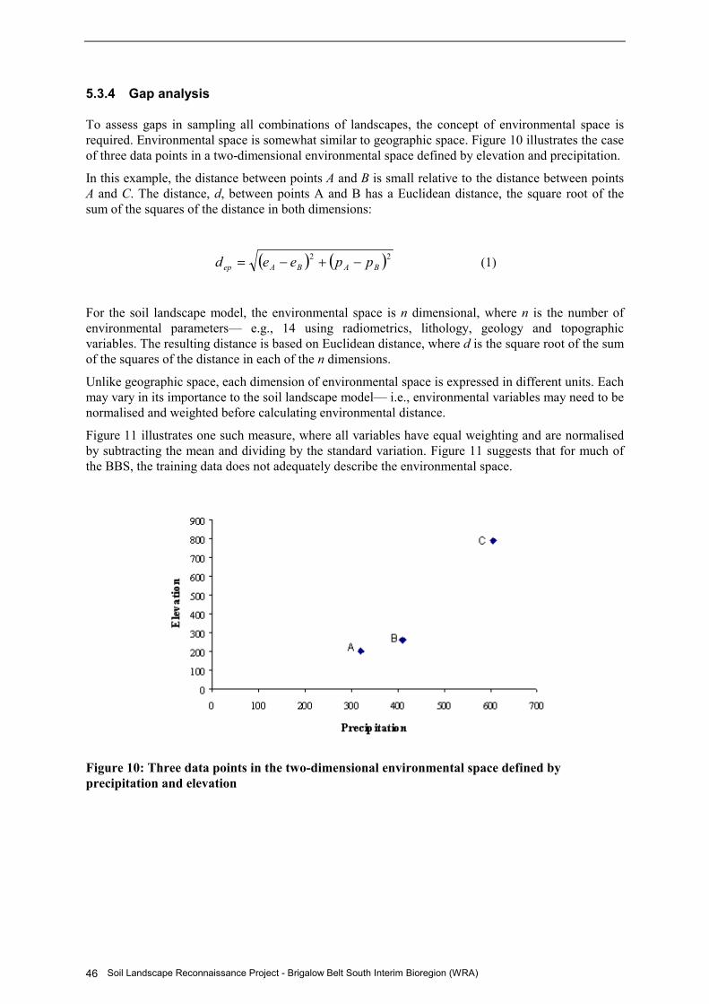
Soil Landscape Reconnaissance Project - Brigalow Belt South Interim Bioregion (WRA)46
5.3.4 Gap analysis
To assess gaps in sampling all combinations of landscapes, the concept of environmental space isrequired. Environmental space is somewhat similar to geographic space. Figure 10 illustrates the caseof three data points in a two-dimensional environmental space defined by elevation and precipitation.
In this example, the distance between points A and B is small relative to the distance between pointsA and C. The distance, d, between points A and B has a Euclidean distance, the square root of thesum of the squares of the distance in both dimensions:
� � � �22BABAep ppeed ���� (1)
For the soil landscape model, the environmental space is n dimensional, where n is the number ofenvironmental parameters— e.g., 14 using radiometrics, lithology, geology and topographicvariables. The resulting distance is based on Euclidean distance, where d is the square root of the sumof the squares of the distance in each of the n dimensions.
Unlike geographic space, each dimension of environmental space is expressed in different units. Eachmay vary in its importance to the soil landscape model— i.e., environmental variables may need to benormalised and weighted before calculating environmental distance.
Figure 11 illustrates one such measure, where all variables have equal weighting and are normalisedby subtracting the mean and dividing by the standard variation. Figure 11 suggests that for much ofthe BBS, the training data does not adequately describe the environmental space.
Figure 10: Three data points in the two-dimensional environmental space defined byprecipitation and elevation

Soil Landscape Reconnaissance Project - Brigalow Belt South Interim Bioregion (WRA) 47
Figure 11: Estimates of the average distance in environmental space of all grid cells in the BBSfrom the points in the training data (excluding lithology and radiometric data)
Note: Darker tone indicates greater environmental distance from sampled environmental spaces. Thisforms the basis for gap analysis.
Considerable delays were encountered due to problems with joint gap analysis due to what transpiredto be a minor data formatting problem that prevented input of the soils model to the gap analysis.This delayed the start of fieldwork for several weeks. In retrospect, it may have been better to startthe fieldwork according to standard soil survey rule sets.
5.3.5 Flexible gap analysis
Due to time constraints, the flexible gap analysis tool was developed from foundations established byS. Ferrier (2001, pers. comm).
Soil profiles for the main fieldwork phase were selected using a portable version of the gap analysismethod initially developed by Ferrier and used for vegetation mapping. The portable gap analysissoftware determines the locations of all existing sampling sites in the study dataset in terms ofweighted environmental variable space. It then calculates the relative distance of all locations in theenvironmental space of the study area to all the sampled locations. A map of the area showing thedegree of sampling in accordance with the environmental variables is then produced. Areas that arenot well represented by the sampled dataset are then selected for sampling. As each sample isselected the portable gap analysis is run again and the map of degree of sampling changes. Essentially

Soil Landscape Reconnaissance Project - Brigalow Belt South Interim Bioregion (WRA)48
the flexible gap analysis tool takes the measure distance from all other sampling points in terms ofenvironmental space (such as portrayed in Figure 11) and represents these distances on a map.
5.3.6 Main fieldwork
Main fieldwork was undertaken from October to December 2001. Extra soil survey staff were calledin to accelerate fieldwork which had been delayed by data management problems.
Four trailer-mounted soil corers were used (where access was available) to excavate soil profiles fordescription to 1.5 metres. Each corer has a jackhammer, propelled by a hydraulic ram, that drives a50 mm-diameter tube into the soil (see Figure 12). Once removed from the tube, each soil core isdescribed using attributes on the WRA Soil Data Card. The corer is well suited to operations in flataccessible areas and a wide range of soils without very hard fragments.
Figure 12: A soil corer in use on the gently undulating plains of the Northern Outwash
Soil landscape details including the calculation for soil attributes (except EPAWC) were entered bythe soil surveyors into the MS Access database for each map sheet area. These were e-mailed or sentby disc to the Soils Quality Officer who arranged for the calculation of EPAWC and entry into themain database.
Access to portable notebook computers with vehicle-based power supplies, and licences for ESRIArcView 3.2 and Spatial Analyst, was organised. Brief training in the use of the SLAP flexible gapanalysis module was arranged, and the system was pressed quickly into service. Many problems wereencountered at first with running such complex software on relatively low-powered computerhardware. However, further development was undertaken, and by the end of the main fieldwork phasethe gap analysis software was working successfully on datasets of around 1,000 km2.
Soil profile points for around 200 locations were determined using flexible gap analysis. This wouldhave been higher except for initial teething problems with hardware limitations and some initialsoftware bugs.
An advantage of the use of in-field computers is that modelled outputs could be field-checked usinglap-tops rather than the time consuming and more laborious approach of having draft maps printed.

Soil Landscape Reconnaissance Project - Brigalow Belt South Interim Bioregion (WRA) 49
5.3.7 Landholder communication protocols
The lengthy landholder consultation protocols used were not well suited to visiting up to 20 sites perday on private land. Consequently it was decided to locate as many sites as possible on publiclyaccessible land, with observations on private land to be undertaken only when communicationprotocols and assistance with making contact could be arranged. Delays were experienced inobtaining official maps showing publicly accessible land, but a travelling stock route and travellingstock reserve map was obtained from NSW Agriculture, which served as a useful guide to someaccessible areas.
Soil surveyors were equipped with various BBS brochures and newsletters and other informationabout soil landscape mapping to aid them in explaining the aims of the project to landholders.
It was not until late September that a formal meeting was held with vegetation and soil survey fieldstaff and the BBS Communications Officer. A protocol and supporting database to facilitatelandholder contact was agreed to be set up, but no further communication was received on thismatter.
Due to pressing deadlines, fieldwork went ahead despite the lack of the streamlined protocol, withsoil surveyors instructed to approach landholders prior to entering private property and to use the‘country code’.
One landholder rang to confirm that soil survey work was actually bona fide in the Coonabarabranarea, as the soil surveyor and technical officer were working on a Sunday.
Most landholders were unaware of the BBS-WRA project, but access refusal was rare.
5.4 POST FIELDWORK
5.4.1 Final modelling
Following the main fieldwork phase, final models were built for each province. Each of the provincemodels (except the Pilliga Outwash and Northern Outwash) was smoothed to minimum mappingareas of 80 pixels or 20 ha. This conforms with the minimum mapping area standards for 1:100 000-scale soil landscape mapping.
5.4.2 Province boundary adjustments
Province boundaries were adjusted so that alluvial, transferral and fan areas adjacent to alluvium andfans of the Northern Outwash and Pilliga Outwash were included in these provinces. Similarly,hillslopes that were included in the outwash provinces were included with hillslopes in adjacentprovinces.
5.4.3 Line work adjustments
Line work was adjusted where necessary, mostly to remove vertical and horizontal boundaries causedby:

Soil Landscape Reconnaissance Project - Brigalow Belt South Interim Bioregion (WRA)50
� Discontinuity in data, e.g., on the boundary between areas covered by radiometrics and areaswithout radiometrics;
� Discontinuities in the available geological mapping; and
� Edges of some existing soil landscape mapping and modelled areas.
Lines were relocated using radiometric and various digital elevation parameters as well as satelliteimagery in consultation with soil surveyors and also, by adhering as much as possible to checked orricher datasets.
A listing of line work changes has been compiled.
5.4.4 Polygon tag changes
In some instances polygons were mis-tagged. This was a consequence of several factors, including:
� serial addition of training areas;
� modelled polygons adjacent to mapped soil landscapes;
� mis-linking of equivalent map units across province boundaries; and
� the model’s occasional inability to always discriminate between whole soil landscapes and facets.
A listing of polygon tag changes has been retained.
5.4.5 Soil profile point data gaps
WRA Soil Data Cards were checked by soil surveyors and were sent to SALIS for scanning into thesystem. The soil profile information was later used to calculate EPAWC.
The locations of WRA Soil Data Cards entered into SALIS were superimposed on the last line workmodel and a count of soil profile observations by soil landscape was undertaken. This provided abasis for planning “mopping-up” fieldwork to address data gaps.
5.4.6 Soil landscape database gaps
A listing of map unit tags was compared with existing database map unit tags. Duplicate databaseentries and missing map unit descriptions in the database were addressed. A list was made of missingdata at facet level for the main predictive surfaces.
5.4.7 “Mopping up” fieldwork
Of the >500 map units and >1,100 facets for the project, it was found that facets lacked soil profiledescriptions. In most cases, soil type was known and confident estimates of important parameterswere made. At the time of writing, “mopping up” fieldwork had been completed for accessible areas.This process was delayed due to staff leave, wet weather and vehicular breakdown. When this soilprofile data becomes available, it will be added to the database and a further edition issued.

Soil Landscape Reconnaissance Project - Brigalow Belt South Interim Bioregion (WRA) 51
5.4.8 Linkage of soil landscape polygons and database
Polygon types were listed against and matched with map unit descriptions. This required correlationand unravelling of map units that were not updated during the modelling process. This was initiallydone on a province-by-province basis.
The map string from the database was then linked to each polygon according to its tag.
Once this process was completed for each province, the provinces were joined and merged into afinal coverage. The map units were then linked to the database. The resulting outputs were checkedfor ‘pinholes’, overlaps and ‘slivers’ and were topologically corrected by a contractor using ESRIArcINFO.
5.4.9 Attribution of soil landscape spatial summary parameters
A set of summary statistics was generated for each soil landscape based on the intersections of soillandscape polygon types with the various spatial surfaces. It included some initial modelling. Each ofthe following statistics is included in the database for generation of summary information and tofacilitate modelling.
The mean positive and negative standard deviations are recommended for use in characterising thetypical parameter range of the soil landscapes. This is because the intersect was completed on thefinal map, which has been smoothed for reliability at 1:100 000 scale. Use of range statisticsnecessarily includes some ‘noise’, which is a feature of natural resource datasets such as soillandscapes. In other words, small areas of included soil landscapes or mapping impurities result inoutliers, which unrealistically extend the range for typical parameters.
For soil landscapes where the standard deviation around the mean is small, it is likely that the soillandscape may have been delineated according to that particular environmental attribute or anotherspatially correlated variable. Where there is a broad range in standard deviation around the mean, thiscan indicate that variation in the soil landscape is related to this or another spatially correlatedvariable. The soil landscape may have had a broad range due to inherent complexity. Alternatively,the extension of the area by modelling may have included areas that may have been better assigned toa different or new landscape.
The summary statistics include: Maximum, Minimum, Range, Mean, Standard Deviation, StandardDeviation plus Mean, Standard Deviation minus Mean.
5.4.9.1 Terrain attributes
� Slope: in degrees, multiplied by 100 and converted to integer.
� Relief: elevation difference within 300 m radius of each cell.
� Relative Elevation Index: pixel elevation less the minimum elevation within 300 m divided bymaximum elevation minus minimum elevation (procedure developed by Dr Goldrick).
5.4.9.2 Temperature attributes
� Annual Mean Temperature ANUCLIM 5.0.
� Temperature Seasonality: coefficient of variation of weekly mean temperature. ANUCLIM 5.0.

Soil Landscape Reconnaissance Project - Brigalow Belt South Interim Bioregion (WRA)52
5.4.10 Database attribution with major variables and calculation of key soil attributes
EPAWC was determined from type profiles (i.e., soil profiles that are considered to be representativeof the main soil type of facets) and estimated using calculations and data in SALIS as described in theMethod section of this report.
Analysis of gaps in the database and checking of outlier values was also completed.
5.4.11 Map and database checking
A number of methods of model checking were explored.
5.4.11.1 Visual comparison of the model with its source maps
The key soil attributes were linked to ArcView 3.2 and evaluated by various staff involved in theproject.
A further planned stage is to have the various attribute surfaces scrutinised and verified by other soilscientists, particularly those familiar with the mapped areas. Initial scrutiny suggests that the surfacesare of sufficient quality for reconnaissance soil landscape mapping in and around the area of thetraining data (Banks, R., Senior Soil Surveyor, DLWC Gunnedah, 2002, pers. comm.). Figure 8shows the comparison of initial model outputs with existing soil landscapes.
A visual comparison of the predicted and training maps for the BBS appears good and adjustmentswere made after examining discrepancies.
Visual examination, however, is not conclusive. Even a poor quality predicted map— e.g., one thathas only about 50% agreement with the training map— can look generally acceptable, but even avery good model may produce a predicted map that differs from the training map when examined indetail.
Maps were produced and checked visually against expected outcomes. This resulted in a list ofqueries that were then checked against the database for clerical errors. Unsolvable discrepancies weredirected to the soil surveyors for solution. In some cases, minor fieldwork was required to solve suchdiscrepancies. Further fieldwork is required to solve all known discrepancies.
5.4.11.2 Logical consistency checking
A technical check for logical consistency of the datasets— e.g., production of pivot tables to checkconsistent features such as well-drained Solodized Solonetz and Lithosols with high EPAWCvalues— has begun. A thorough check will be undertaken by DLWC as part of a planned SALIS dataaudit. Discrepancies to date have been few and easily fixed by telephone queries.

Soil Landscape Reconnaissance Project - Brigalow Belt South Interim Bioregion (WRA) 53
5.4.11.3 Misclassification checking
Analysis in areas of existing soil landscape mapping in the Liverpool Plains and Ranges allowed theinitial predicted surface soil landscapes to be compared with existing soil landscape maps of theCurlewis and Blackville 1:100 000 map sheets (Banks 1995;1998). In the case of BBS regressiontrees, the misclassification rates were 26 and 29 per cent for the radiometric and lithological trees,respectively. Given the ‘noise’ inherent in any natural dataset, and the expected variations within thesoil landscapes (see below), this result seems acceptable. It should be noted that similar rates ofmisclassification are typical for land resource assessment and that soil landscape maps are typicallyfound to predict most physical soil attributes in around 17 cases out of 20 (Dewar 1996).
There are several reasons to expect such discrepancies between the modelled and pre-existing maps,even in the best of circumstances. In most cases, a soil surveyor and a classification tree will predictthe conceptual basis for each soil landscape in slightly different terms. For example, a soil surveyormight define a soil landscape with granitic parent material, steep to very steep slopes and low meanannual rainfall. The same soil landscape may be defined by the classification tree as those areas witha certain radiometric signal, slopes greater than 22� and mean annual precipitation below 587 mm.While these differences may seem trivial, they will lead to variations in the final product, mostnotably in the placement of boundaries.
Further, in delineating the boundaries and extent of this soil landscape, the classification tree followsprecise, objective rules. The soil surveyor, on the other hand, is more likely to delineate the soilboundary through the subjective assessment of information from API, geology maps, topographicmaps and climate maps. Moreover, it is often the case that two experienced soil surveyors will makeslightly different assessments of the data and thus delineate the boundaries differently. This is not tosay that the boundaries resulting from the classification tree are necessarily more accurate or betterthan those drawn by surveyors, but they are more precise and objective. On the other hand, it is alsopossible that where discrepancies exist, that the model has more accurately characterised the natureof a soil landscape than the surveyor. An advantage of the modelling approach is that the method isboth quantifiable and reproducible.
In two areas on the Curlewis 1:100 000 soil landscape map sheet, the model appeared to predict soillandscape boundaries better than the original mapping. This was mostly the result of usingradiometric data that was not available at the time of the original survey.
The predictive maps presented here are an evaluation of the technique based on presently availabledata in areas that are challenging for environmental modelling, especially where environmentalsurfaces are imperfect or of insufficient resolution or incomplete.
5.4.11.4 Evaluation against the independent dataset
Given expected differences between the training and predicted maps, it seems better to test thepredictions through field observation and air photo interpretation. The question to be asked for eachobservation is� “are the characteristics of the site consistent with the predicted soil landscape?”
In evaluating this question, it needs to be recognised that within each soil landscape, there will bevariations in most of its characteristics. For example, a single soil type may occur in a number of soillandscapes as either dominant or minor facets. The test of prediction must therefore be� “is itreasonable that the observed soil type should occur in this predicted soil landscape?”, not� “is theobserved soil the dominant type for this predicted soil landscape?” The latter criterion, used in asimilar study by Bui et al. (1999), is too restrictive given typical heterogeneity of soil landscapes.
The independently gathered soil profile dataset is being gathered at various fauna and flora surveysites. This process has been delayed to allow completion of the main map and database delivery.

Soil Landscape Reconnaissance Project - Brigalow Belt South Interim Bioregion (WRA)54
5.4.11.5 Evaluation of training area representativeness
No matter how well a model predicts soil classes in the vicinity of the training data, one can expectthat the accuracy of the model predictions will decrease in environments dissimilar to that in which itwas trained. This raises the problem of defining the degree of dissimilarity between the environmentof the training area and the environment of the areas that were modelled. Some areas were modelledin much more detail than was warranted, and some tagged inaccurately. While field-checking hasattempted to assign such areas to correct landscapes, not all can be checked off, so best estimates hadto be made.
In future projects, the flexible gap analysis tool could be potentially used to model areas that are leastsimilar to already mapped areas. In the current study, this opportunity was missed because gapanalysis technology was not available at the time of training area selection.
5.4.12 Allocation of soil landscapes to 15 km buffer
DLWC is currently completing linework and database entry of soil landscapes for the 15 km bufferfor NPWS. This buffer was dropped from the original proposal due to budget cuts to the project.
The 15 km buffer is being mapped and described independently from the main project using existingsoil landscape information (where available) and on-screen digitising of estimated soil landscapeboundaries using TM, geological, radiometric and contour information. Both soil landscapeboundaries and information entered in the database, for new mapping areas, are estimates made bythe soil surveyor and have not been field checked. As such, caution should be taken when using thecoverages or soils information for these areas.
5.4.13 Design of Web products
Preliminary design of a series of Internet-served maps of this study and their associated map unitdescriptions are planned, but cannot be carried out efficiently at time of writing. This is based on aWorld Wide Web environment where the user can select various views of the database along with anumber of checked maps. This process will take advantage of SALIS’s developing ability to storespatial information and allow it to be viewed using an Internet spatial viewer. At present, this isawaiting approval for development of SALIS to accept the fields used in the MS Access database. Asan organisation, DLWC is committed to producing interactive web products. It is expected that such asystem will be in place early next financial year.
5.4.14 Access to information
This document is accompanied by a compact disk, which contains the MS Access map unit database,and shape file of the final mapped output that can be used in ESRI and other GIS platforms.
Distribution is provided on the basis that the data is not to be handed to third parties beyond the BBS-WRA project without written permission and appropriate acknowledgment.
For further copies of the CD or the dataset in other formats, please request via e-mail to thefollowing address� [email protected].

Soil Landscape Reconnaissance Project - Brigalow Belt South Interim Bioregion (WRA) 55
Requests for access to publicly available soil profile information in SALIS should also be made via e-mail to the same address� [email protected].
5.4.15 Feedback
Feedback on this report or any aspect of the project is welcome. Such feedback should be sent to thefollowing e-mail address— [email protected].

Soil Landscape Reconnaissance Project - Brigalow Belt South Interim Bioregion (WRA)56
6.1 SOIL PROFILE INFORMATION
Soil profiles descriptions were collected or collated for the BBS area. Maps 1 and 2 show thedistribution of soil profile sites from both newly mapped areas and existing soil landscape coverage.The data is held in the NSW Soil And Land Information System (SALIS) and is accessible by e-mailrequest to [email protected].
Once the final results of the project are made public, the soil point information will also be madeavailable via DLWC’s Soil Profile Attribute Data Environment (SPADE) spatial viewer on theInternet at the following Web address: http://spade.dlwc.nsw.gov.au.
6.2 MAP COVERAGES AND DATABASE
6.2.1 Soil landscape coverage
A complete, seamless coverage of soil landscapes for the entire BBS area (Map 5) has beencompleted. Over 500 soil landscapes have been compiled both from existing draft and published soillandscapes and from reconnaissance level 1:100 000 scale soil landscape mapping. Furthermore, over1,100 facets with soil attribute data were described, which can be linked with DEMs to produceenhanced 1:25 000-scale coverage if required. This coverage and the matching database have beendistributed to major stakeholders for modelling purposes.
6.2.2 Other coverages
Map coverages and surfaces used as part of the modelling program (see Tables 9 and 10) includeClimatic Surfaces (Maps 6a through d), DEMs (Maps 7a through f), and derived Great Soil Group,GSG (Map 9). These were provided to Planning NSW staff and NPWS vegetation modellers inFebruary 2002.
6.3 SOIL ATTRIBUTE THEMES

Soil Landscape Reconnaissance Project - Brigalow Belt South Interim Bioregion (WRA) 57
Examples of current soil attribute themes for Fertility (Map 11), Soil Profile Depth (Map 12),Effective Rooting Depth (Map 13), Estimated Plant Available Waterholding Capacity (Map 14),Drainage (Map 15) and Soil Regolith Stability (Map 10) for dominant facets have been generated.These themes were compiled from the soil landscape coverage and information in the map unitdatabase and are displayed according to the dominant facet for each soil landscape. They are likely tobe revised as the modelling process evolves.
6.4 SOIL LANDSCAPE DATABASE
An MS Access database was produced that detailed descriptions for each soil landscape in the BBS.It includes information on the main soil attributes useful for vegetation modelling (e.g., fertility,EPAWC, ERD and drainage). Other soil and landscape information (e.g., soil type, soil and landscapelimitations) was also recorded for each soil landscape, making the data useful for many purposesother than vegetation modelling.
6.5 USE OF DATA
These maps and the associated database provide a guide to the distribution and assessment of soillandscape attributes across the BBS. The maps should be used only at 1:100 000 scale or smaller andshould not be used for any other purpose than broad regional vegetation modelling purposes.Enhanced resolution of these soil attributes can be gained through linkage with digital elevationmodels. This will be undertaken by NPWS as required for modelling purposes. The soil attributethemes generated will assist in the modelling of:
� Biodiversity assessment;
� Potential and current forest community modelling;
� Fauna modelling;
� Rare flora species modelling;
� Centres of endemism;
� Response to disturbance;
� Plantation potential on cleared private land; and
� Industry development opportunities (e.g., intensification).
6.6 METADATA
Individual metadata statements conforming to the ANZLIC Page 0 standard have been prepared forthe project, its associated MS Access database, and all maps in this report. These statements havebeen submitted for inclusion in the NSW Natural Resource Data Directory (available on the Internetathttp://www.canri.nsw.gov.au/nrdd).

Soil Landscape Reconnaissance Project - Brigalow Belt South Interim Bioregion (WRA)58
6.7 OVERLAYS
A transparent overlay containing road and town information has been provided with the appendices.Issues of scale mean that this overlay only matches with maps 5 and 9 through 16.

Soil Landscape Reconnaissance Project - Brigalow Belt South Interim Bioregion (WRA) 59
7.1 ARE THE DATA AND CONCLUSIONS ROBUST AND RELIABLE?
No matter how well a model predicts soil classes in the vicinity of the training data, the accuracy ofthe model predictions is likely to decrease in environments dissimilar to that in which it was trained.This raises the problem of defining the degree of dissimilarity between the environment of thetraining area and the environment of the areas that were modelled. Some areas were modelled inmuch more detail than warranted, and some were tagged inaccurately. While field checking attemptedto assign such areas to correct landscapes, not all could be checked in time, so best estimates weremade. The results of the model were significantly accurate at the reconnaissance scale used. This isfurther outlined in Section 7.5 on the following page.
In future projects, the portable gap analysis tool could be used to model areas that are least similar toalready mapped areas. In the current study, this could not be done because the gap analysistechnology was not available at the time of training area selection.
7.2 HOW DO THE OUTPUTS FROM THIS PROCESS COMPARE WITHOTHER SOIL LANDSCAPE MAPPING PROJECTS?
The Brigalow Belt South Interim Bioregion was mapped faster and in a more objective manner thanthe Southern CRA and North-East CRA soil mapping projects.
The quality of outputs tends to be more variable than the CRA soil mapping projects, dependingmostly on the quality of environmental variables available. The mapping technique is more rapid thansoil landscape mapping, but does not result in as high a quality or as versatile a product. This isessentially because there is less time available for detailed checking that the traditional soil landscapemapping process enjoys. Soil landscape mapping also includes laboratory data and assessments ofsoil limitations. Neither of these was included in this project.
7.3 WAS THE PROJECT VARIATION SUCCESSFUL?
The project variation was successful in that it overcame time constraints and included thedevelopment of the flexible gap analysis tool, a hybrid approach in which:
� Soil surveyors are able to carry out their own sample site selection;
� Air photo interpretation is used as a moderating layer over the entire study area; and
� Soil landscapes can be modelled according to rule sets determined in-the-field.
This process is expected to result in better maps and datasets, and is recommended for futuremapping projects of a similar nature. In particular, inclusion of limited soil testing for key plantgrowth variables is expected to increase the utility of the resulting dataset.

Soil Landscape Reconnaissance Project - Brigalow Belt South Interim Bioregion (WRA)60
7.4 HOW WILL THE PROJECT BE USEFUL TO THE ASSESSMENT?
This project was undertaken to fill the substantial gap in soil knowledge within the BBS. Thisinformation was required by the joint BBS vegetation mapping project by the end of March 2002. Asnoted previously, mapped soil attributes are particularly important in terms of the vegetation mappingproject in the BBS as the terrain is mostly subdued and soils assume a greater influence indetermining plant species distribution. Soils information is a fundamental precursor to subsequentvegetation mapping so it was essential that soils information be provided as soon as practicable.
7.5 MODEL TESTING ACCURACY
7.5.1 Distribution and Descriptive Statistics
An assessment was undertaken in order to determine the accuracy of the model. The requiredoutcomes of the assessment were to determine relationships between results, separated by into theprovinces of Liverpool Plains, Northern basalts, Northern Outwash, Pilliga and Pilliga Outwash asoutlined in pages 43-45 of this report.
In order to test the accuracy of the model, 180 independent field soil profiles were collected on astratified random basis by 1:100 000 map sheets across all new mapping areas and compared toequivalent points determined by the model. The values of effective rooting depth, estimated potentialavailable water capacity, fertility, A1 (topsoil) texture and regolith were extracted from both theprofiles and the model and were compared. These were grouped into ranges as shown in Tables 11through 15 with the exception of regolith, which is already grouped.
Table 11: Effective Rooting Depth ranges for calculation of accuracyas per Isbell (1996)
Grouping (Range) Value Classification1 0 – 0.25 Very Shallow2 >0.25 – 0.5 Shallow3 >0.5 – 1.0 Moderate4 <1.0 – 1.5 Deep5 >1.5 Very Deep to Giant6 Disturbed
Table 12: EPAWC ranges for calculation of accuracy
Grouping (Range) Value Classification1 1-140 Very Low2 141-300 Low3 301-550 Moderate4 551-800 High5 800-1500 Very High
Table 13: Fertility ranges for calculation of accuracy

Soil Landscape Reconnaissance Project - Brigalow Belt South Interim Bioregion (WRA) 61
Grouping (Range) Classification1 Very Low2 Low3 Moderate4 High5 Very High
Table 14: A1 Texture ranges for calculation of accuracyas per Isbell (1996)
Grouping (Range) Texture Group Texture Grades1 Sands Sand, Loamy Sand, Clay Sand2 Loams Sandy Loam, Loam3 Clay Loams Sandy Clay Loam, Clay Loam, Silty
Clay Loam4 Clay Sandy Clay, Loamy Clay, Silty Clay,
Medium Clay, Heavy Clay
Table 15: Regolith ranges for calculation of accuracy
Grouping (Range) Value Classification1 R1 High coherence, low sediment delivery potential2 R2 Low coherence, low sediment delivery potential3 R3 High coherence, high sediment delivery potential4 R4 Low coherence, high sediment delivery potential
A rating was given to point results on the basis of how well each matched the observed field resultcategory. For all values other than regolith, a match was given a score of 1. If the groupings did notmatch but were one field removed from a match, a score of 0.5 was assigned. All other result’s scored0. Regolith values were assigned either 1 for a match or 0 for a mismatch due to the unranked natureof the data. The sum of these scores gave a possible overall score out of 5 for each point. Wherelimitations existed in the database, due to the absence of suitable facets in many of the soillandscapes, the soil type/facet that best matched the facet from the model was used.
Accuracy values and statistics were determined at the levels: a) match versus mismatch; and b) matchversus partial match versus no match. These values were determined using the points ranking systemabove whereby a return of 1 indicates a match, 0.5 as a partial match and 0 as a non match. TheMode, Median, Mean and Standard Deviation were determined using the Descriptive Statistics tool inEXCEL. Mean was not applicable for Regolith as the data is nominal.
The overall accuracy using the match/partial match/no match system is shown in Table 21 on page66. Accuracy for match/no match is also shown for each attribute in the same table. Accuracy for thedifferent fields varied across provinces as can be seen in figures 13 through 17 on the followingpages. All figures bar Regolith show match and partial match. The remaining percentage is for nomatch. Regolith values are only match and no match for reasons outlined above. The distribution ofmatches with regards to a score out of five is shown in Figure 18 on page 64. The distribution ofresults for match/partial match/no match is shown for each attribute in maps 16a - e in Appendix 3.

Soil Landscape Reconnaissance Project - Brigalow Belt South Interim Bioregion (WRA)62
Figure 13: Percentage accuracy for topsoil texture across all provinces
Figure 14: Percentage accuracy for Effective Rooting Depth across all provinces
LiverpoolPlains
Northernbasalts
NorthernOutwash Pilliga
PilligaOutwash
40.74
48.15
60.00
30.00
80.95
9.52
34.43
50.82
50.00
30.00
0.00
10.00
20.00
30.00
40.00
50.00
60.00
70.00
80.00
90.00
100.00
Perc
enta
ge
Province
Partial MatchMatch
LiverpoolPlains
Northernbasalts
NorthernOutwash Pilliga
PilligaOutwash
0.00
10.00
20.00
30.00
40.00
50.00
60.00
70.00
80.00
90.00
100.00
Perc
enta
ge
Province
Estimated Rooting Depth
Partial MatchMatch
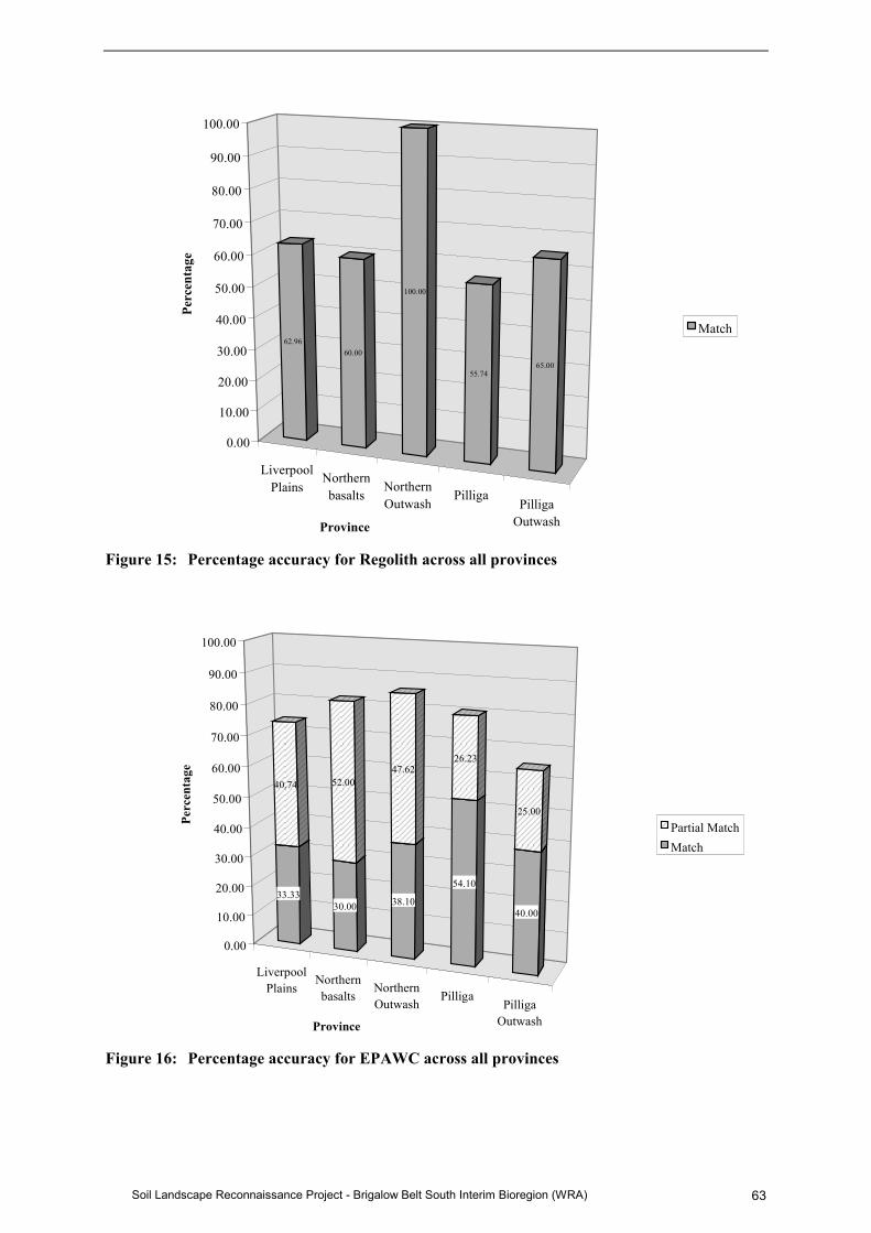
Soil Landscape Reconnaissance Project - Brigalow Belt South Interim Bioregion (WRA) 63
Figure 15: Percentage accuracy for Regolith across all provinces
Figure 16: Percentage accuracy for EPAWC across all provinces
LiverpoolPlains
Northernbasalts
NorthernOutwash
PilligaPilliga
Outwash
62.9660.00
100.00
55.7465.00
0.00
10.00
20.00
30.00
40.00
50.00
60.00
70.00
80.00
90.00
100.00
Perc
enta
ge
Province
Match
LiverpoolPlains
Northernbasalts
NorthernOutwash
PilligaPilliga
Outwash
33.33
40.74
30.00
52.00
38.10
47.62
54.10
26.23
40.00
25.00
0.00
10.00
20.00
30.00
40.00
50.00
60.00
70.00
80.00
90.00
100.00
Perc
enta
ge
Province
Partial MatchMatch

Soil Landscape Reconnaissance Project - Brigalow Belt South Interim Bioregion (WRA)64
Figure 17: Percentage accuracy for Fertility across all provinces
Figure 18: Percentage distribution of results showing percentage of matches for all for allmain attributes from each province as a score out of 5. The score is given by the number ofmatches (1) and partial matches (0.5) added for each of the tested parameters; ERD, A1texture, EPAWC, Regolith and Fertility as outlined above.
LiverpoolPlains
Northernbasalts
NorthernOutwash
PilligaPilliga
Outwash
37.04
48.15
56.00
20.00
85.71
4.76
55.74
31.15
55.00
35.00
0.00
10.00
20.00
30.00
40.00
50.00
60.00
70.00
80.00
90.00
100.00
Perc
enta
ge
Province
Partial MatchMatch
0
5
10
15
20
25
30
35
40
Liverpool Plains Northern basalts Northern Outwash Pilliga Pilliga Outwash
Province
Perc
enta
ge o
f Pro
files
0.00
0.50
1
1.5
2
2.5
3
3.5
4
4.5
5

Soil Landscape Reconnaissance Project - Brigalow Belt South Interim Bioregion (WRA) 65
Table 16: Liverpool Plains province descriptive statistics for each of the test parameters andthe final score. Test Parameter results are based on the groupings of data as outlined in Tables11 through 15 and the final score as outlined on page 61
Mean Median Mode Standard DeviationA1 Texture 2.89 3.00 4.00 1.09ERD 4.96 5.00 5.00 0.19EPAWC 3.52 3.00 3.00 1.34Regolith Class N/A R3 R3 N/AFertility 2.89 3.00 3.00 0.97Final Score 3.24 3.50 3.50 0.97
Table 17: Northern Basalts province descriptive statistic of each of the test parameters andthe final score. Test Parameter results are based on the groupings of data as outlined in Tables11 through 15 and the final score as outlined on page 61
Mean Median Mode Standard DeviationA1 Texture 2.66 3.00 4.00 1.15ERD 3.96 4.00 5.00 0.99EPAWC 2.06 2.00 2.00 1.11Regolith Class N/A R3 R3 N/AFertility 3.24 3.00 5.00 1.57Final Score 3.17 3.00 3.00 1.10
Table 18: Northern Outwash province descriptive statistic for each of the test parameters andthe final score. Test Parameter results are based on the groupings of data as outlined in Tables11 through 15 and the final score as outlined on page 61
Mean Median Mode Standard DeviationA1 Texture 3.81 4.00 4.00 0.60ERD 4.95 5.00 5.00 0.22EPAWC 4.05 4.00 4.00 0.74Regolith Class N/A R3 R3 N/AFertility 3.14 3.00 3.00 0.48Final Score 4.33 4.50 4.50 0.81
Table 19: Pilliga province descriptive statistic for each of the test parameters and the finalscore. Test Parameter results are based on the groupings of data as outlined in Tables 11through 15 and the final score as outlined on page 61
Mean Median Mode Standard DeviationA1 Texture 2.05 2.00 1.00 0.98ERD 4.68 5.00 5.00 0.84EPAWC 2.89 3.00 3.00 1.01Regolith Class N/A R3 R3 N/AFertility 2.35 2.00 2.00 0.89Final Score 3.35 3.50 3.50 1.13

Soil Landscape Reconnaissance Project - Brigalow Belt South Interim Bioregion (WRA)66
Table 20: Pilliga Outwash Descriptive Statistic for each of the test parameters and the finalscore. Test Parameter results are based on the groupings of data as outlined in Tables 11through 15 and the final score as outlined on page 61
Mean Median Mode Standard DeviationA1 Texture 2.10 2.00 2.00 0.97ERD 4.85 5.00 5.00 0.37EPAWC 3.30 3.00 3.00 0.98Regolith Class N/A R3 R3 N/AFertility 1.85 2.00 2.00 0.75Final Score 3.40 3.25 3.00 1.15
Table 21: Accuracy for each of the provinces for all five parameters expressed as apercentage
LiverpoolPlains
NorthernBasalts
NorthernOutwash
Pilliga PilligaOutwash
Overall
Match and Partial Match 64.8 63.4 86.7 67.1 68 68.1Match 48.9 60 80 54.83 58 55.9
7.5.2 Cohen’s Kappa
A common measure of agreement is the sum of the diagonal entries in the error matrix divided by thetotal number of observations (in this case N=180). This is the proportion of samples placed into thesame category by the model and from the field measurements, Po:
��
�
r
1iii Nn Po
However, this measure ignores agreement between the methods that may have been due to chance.The level of agreement due to chance is given by:
��
���
r
1iii Nnn
N1Pc
This formula is based on the marginal totals ni+ and n+i of the rows and columns. This formula alsoassumes that the marginal totals are independent which may not be the case for ordinal categories.There may be considerable difference between the observed and chance agreement. Cohen’s Kappa,�, is a statistic that measures this:
Pc1Pc-Po
�
��
When there is perfect agreement between the field and model values, Po = 1, so the maximumpossible difference between the observed and chance agreements will be (1 – Pc). The kappa statisticthus gives the ratio of the excess of the observed agreement over chance agreement. Fitzgerald andLees (1994) explain this as “The kappa statistic tests the null hypothethis that two independentclassifiers do not agree on the rating or classification of the same object”.
A rule of thumb (Landis and Koch 1977) for interpreting various kappa values is shown in Table 22on the following page. The strength of agreement indicates the probability of a reference point value

Soil Landscape Reconnaissance Project - Brigalow Belt South Interim Bioregion (WRA) 67
being the same as the model value. The weighted form of the Cohen’s Kappa statistic isrecommended for use with ordinal categories. This is described by Fleiss (1981). Everitt (1991) givesan estimate of the asymptotic standard error. This was used to calculate 95% confidence intervals andp-values.
Table 22 Strength of Agreement ratings for Cohens Kappa Statisticfrom Landis and Koch (1977)
Kappa Strength of Agreement
0.00 poor0.00–0.20 slight0.21–0.40 fair0.41–0.60 moderate0.61–0.80 substantial0.81–1.00 almost perfect
Kappa was significant for all characteristics as shown in Table 23 below. Most of the soil propertiesmeasured for the value of kappa fell into the “fair” to “moderate” range. For ERD, the modelledvalues showed only slight concordance with the observed data.
Table 23 Summary of agreement statistics for the five soil characteristics. Po is the observedprobability of agreement, Pc is the probability of agreement due to chance, kappa is the valueof Cohen’s Kappa statistic. This has been weighted for the first four ordinal categories. Theunweighted form of kappa was applied to regolith as is the asymptotic standard error (ase).
Po Pc kappa ase p-value 95% conf. interval
ERD 0.87 0.85 0.169 0.073 0.02 0.026 0.311EPAWC 0.79 0.67 0.365 0.049 <0.001 0.269 0.460A1 texture 0.79 0.58 0.494 0.047 <0.001 0.403 0.586Fertility 0.84 0.68 0.511 0.049 <0.001 0.415 0.607Regolith 0.64 0.43 0.367 0.055 <0.001 0.248 0.486
7.5.3 Synthesis and Conclusion of Accuracy Tests
The weakest Cohen’s Kappa result was Effective Rooting Depth (“slight” range). This can beexplained by a high probability of a match (85%) by chance due to the poor spread of the data. Alarge portion of the results fell in the very deep to giant range (soil depth greater than 1.5m). As theboreholes were dug to 1.5m, any sample with Rooting Depth greater than this fell into this range. Allother results were in the “fair” to “moderate” range, the strongest match being Fertility (84%probability of a match, 68% probability by chance). Regolith had the lowest probability of a result bychance (43%) and overall (64%).
Results show that there is variation in the accuracy of the model for different provinces. There aremany possibilities as to the reason that this occurred. Changed values due to incorrect classification

Soil Landscape Reconnaissance Project - Brigalow Belt South Interim Bioregion (WRA)68
are one possible explanation for incorrect results, particularly with regard to regolith values. This iscurrently under review and changes have been made. It was observed that results that were mostlyincorrect had been extrapolated across large distances ie the model had used soil informationdescribed at one location to match soils several 1:100 000 map sheets away.
The quality control check will satisfy many of the concerns raised by various Stakeholders, whoexpressed various sentiments regarding the accuracy and usefulness of the soil maps produced by theproject. Most areas of the model (eg Northern Outwash) have mapped accurately while other areashave not (eg Liverpool Plains). The majority of ground truthed areas (68.1%) were consistent withmodel values. The check was done using 180 soil profiles, which were selected on a stratified randombasis in areas without Soil Landscape mapping covering each of the unpublished map sheets in theregion.
This provides an indication of the accuracy of the model over different provinces, which weremapped using different environmental attribute weightings. Considering the broad scalereconnaissance level of mapping used (1:100 000), mapping could only be tested at a generallandscape level as opposed to the 14,420 individual polygons, as excessively extensive fieldworkwould be required to check the data at any resolution greater than that undertaken.
Soil landscape mapping is an interpretive process and as such, is based on the soil surveyoridentifying the relationship between soils and landscapes properties. It is these key relationships thatwere identified by the soil surveyors and incorporated into the model.
Higher resolution data can be viewed for each province using the provided ArcVIEW shape files andattribute tables. All Individual profiles described in the course of this project will be made availablefor viewing through SPADE (located at http://spade.dlwc.edu.au) in the near future.
The process undertaken in this project is similar to that of a Soil Landscape Map. The production of aSoil Landscape map over this size area (54 000 ha) usually requires 21 person years to produce thefinal output while this project required approximately 5 person years to complete. The accuracy ofSoil Landscape mapping ranges from 73 to 87 % accurate based on a range of soil propertiesincluding depth, texture, plasticity and Organic Matter content (Dewar et al., 1996). The cost of thisproject worked out at around $9.35 km2. This equates favourably with figures provided by McKenzie(1991), who states the figure of $28.00 km2 (1988 value quoted) as being sufficient to provide acrude prediction of soil land characteristics at a nominated location
All minor alterations and typographical errors reported have been edited. An overlay has beenincluded in the appendices showing road network and towns in the region.
The Department of Land and Water Conservation Soil Information Systems Unit are the custodian ofthis data set. As errors become known, efforts will be made where resources permit, to update thequality of the dataset. Users are requested to contact [email protected] to provide feedback andinformation regarding inconsistencies, errors, omissions or updates that will enhance the data set.