software trajectory analysis: an empirically based method for...
TRANSCRIPT

.
Dissertation proposal:
Software Trajectory Analysis:
An empirically based method for
automated software process discovery
Pavel Senin
Collaborative Software Development Laboratory
Department of Information and Computer Sciences
University of Hawaii
Committee:
Philip M. Johnson, Chairperson
Kyungim Baek
Guylaine Poisson
Henri Casanova
Daniel Port
CSDL Technical Report 09-09
http://csdl.ics.hawaii.edu/techreports/09-09/09-09.pdf
August 2009
Contents
1 Introduction 3
1.1 Motivation . . . . . . . . . . . . . . . . . . . . . . . . . . . . . . . . . . . . . 3
1.2 Proposed contribution . . . . . . . . . . . . . . . . . . . . . . . . . . . . . . 4
1.3 Roadmap . . . . . . . . . . . . . . . . . . . . . . . . . . . . . . . . . . . . . 5
2 Related work 6
2.1 Software process discovery . . . . . . . . . . . . . . . . . . . . . . . . . . . . 6
2.1.1 Process discovery through Grammar Inference . . . . . . . . . . . . . 7
2.1.2 Incremental Workflow Mining with Petri Nets . . . . . . . . . . . . . 9
2.1.3 Reference model for Open Source Software Processes Discovery . . . 11
2.2 Mining software repositories . . . . . . . . . . . . . . . . . . . . . . . . . . . 11
2.2.1 Mining evolutionary coupling and changes . . . . . . . . . . . . . . . 12
2.2.2 Ordered change patterns . . . . . . . . . . . . . . . . . . . . . . . . . 13
2.2.3 Usage patterns . . . . . . . . . . . . . . . . . . . . . . . . . . . . . . 13
2.3 Temporal data mining . . . . . . . . . . . . . . . . . . . . . . . . . . . . . . 14
2.3.1 Piecewise Aggregate Approximation (PAA) . . . . . . . . . . . . . . . 15
2.3.2 Symbolic Aggregate approXimation (SAX) . . . . . . . . . . . . . . . 16
2.3.3 Symbolic series, temporal models, concepts, and operators . . . . . . 18
2.3.4 Temporal data models . . . . . . . . . . . . . . . . . . . . . . . . . . 18
2.3.5 Temporal concepts . . . . . . . . . . . . . . . . . . . . . . . . . . . . 19
2.3.6 Temporal operators . . . . . . . . . . . . . . . . . . . . . . . . . . . . 19
2.3.7 Temporal patterns and indexing . . . . . . . . . . . . . . . . . . . . . 21
2.3.8 Time points patterns . . . . . . . . . . . . . . . . . . . . . . . . . . . 22
2.3.9 Time interval patterns . . . . . . . . . . . . . . . . . . . . . . . . . . 23
2.3.10 Apriori algorithm . . . . . . . . . . . . . . . . . . . . . . . . . . . . . 26
1

3 Software Trajectory: a software process mining framework. 28
3.1 Current state of development . . . . . . . . . . . . . . . . . . . . . . . . . . 28
3.1.1 Temporal data indexing . . . . . . . . . . . . . . . . . . . . . . . . . 31
3.1.2 Index database design . . . . . . . . . . . . . . . . . . . . . . . . . . 32
3.2 TrajectoryBrowser . . . . . . . . . . . . . . . . . . . . . . . . . . . . . . . . 34
3.3 Future development roadmap . . . . . . . . . . . . . . . . . . . . . . . . . . 35
4 Experimental evaluation 37
4.1 Review of evaluation strategies . . . . . . . . . . . . . . . . . . . . . . . . . 38
4.1.1 The two paradigms . . . . . . . . . . . . . . . . . . . . . . . . . . . . 38
4.1.2 Mixed methods and Exploratory research . . . . . . . . . . . . . . . . 39
4.2 Software Trajectory approach evolution . . . . . . . . . . . . . . . . . . . . . 39
4.3 Software Trajectory case studies and evaluation design . . . . . . . . . . . . 40
4.4 Pilot study . . . . . . . . . . . . . . . . . . . . . . . . . . . . . . . . . . . . 41
4.4.1 Clustering of the Hackystat Telemetry streams . . . . . . . . . . . . . 43
4.4.2 Sequential patterns search . . . . . . . . . . . . . . . . . . . . . . . . 43
4.5 Public data case study . . . . . . . . . . . . . . . . . . . . . . . . . . . . . . 45
4.6 Classroom study . . . . . . . . . . . . . . . . . . . . . . . . . . . . . . . . . 47
4.6.1 Classroom study design . . . . . . . . . . . . . . . . . . . . . . . . . 48
4.6.2 Personal software process discovery . . . . . . . . . . . . . . . . . . . 50
4.6.3 Team-based software process discovery . . . . . . . . . . . . . . . . . 50
5 Summary and Future Directions 53
5.1 Contribution . . . . . . . . . . . . . . . . . . . . . . . . . . . . . . . . . . . . 53
5.2 Estimated Timeline . . . . . . . . . . . . . . . . . . . . . . . . . . . . . . . . 53
6 Appendices 55
6.1 Classroom case study interview design . . . . . . . . . . . . . . . . . . . . . 55
6.1.1 Software Trajectory evaluation interview questionnaire . . . . . . . . 56
6.1.2 Software Trajectory consent form . . . . . . . . . . . . . . . . . . . . 57
2

Chapter 1
Introduction
1.1 Motivation
A software process is a set of activities performed in order to design, develop and maintain
software systems. Examples of such activities include design methods; requirements collec-
tion and creation of UML diagrams; requirements testing; and performance analysis. The
intent behind a software process is to structure and coordinate human activities in order to
achieve the goal - deliver a software system successfully.
Much work has been done in software process research resulting in a number of industrial
standards for process models (CMM, ISO, PSP etc. [10]) which are widely accepted by many
institutions. Nevertheless, software development remains error-prone and more than half of
all software development projects ending up failing or being very poorly executed. Some of
them are abandoned due to running over budget, some are delivered with such low quality
or so late that they are useless, and some, when delivered, are never used because they do
not fulfill requirements. The cost of this lost effort is enormous and may in part be due to
our incomplete understanding of software process.
There is a long history of software process improvement through proposing specific pat-
terns of software development. For example, the Waterfall Model process proposes a sequen-
tial pattern in which developers first create a Requirements document, then create a Design,
then create an Implementation, and finally develop Tests. The Test Driven Development
process proposes an iterative pattern in which the developer must first write a test case,
then write the code to implement that test case, then refactor the system for maximum
clarity and minimal code duplication. One problem with the traditional top-down approach
to process development is that it requires the developer or manager to notice a recurrent
3
pattern of behavior in the first place [10].
In my research, I will apply knowledge discovery and data mining techniques to the
domain of software engineering in order to evaluate their ability to automatically notice
interesting recurrent patterns of behavior. While I am not proposing to be able to infer a
complete and correct software process model, my system will provide its users with a formal
description of recurrent behaviors in their software development. As a simple example,
consider a development team in which committing code to a repository triggers a build of
the system. Sometimes the build passes, and sometimes the build fails. To improve the
productivity of the team, it would be useful to be aware of any recurrent behaviors of the
developers. My system might generate one recurrent pattern consisting of a) implementing
code b) running unit tests, c) committing code and d) a passed build: i → u → c → s, and
another recurrent pattern consisting of a) implementing code, b) committing code, and c) a
failed build: i → c → f . The automated generation of these recurrent patterns can provide
actionable knowledge to developers; in this case, the insight that running test cases prior to
committing code reduces the frequency of build failures.
Although the latest trends in software process research emphasize mining of software
process artifacts and behaviors [23] [45] [39] [45], to the best of my knowledge, the approach
I am taking has never been attempted. This may be partly due to the lack of means of
automated, real-time data collection of fine-grained developer behaviors. By leveraging the
ability of the Hackystat system [25] to collect such a fine grained data, I propose to extend
previous research with new knowledge that will support improvements in our understanding
of software process.
1.2 Proposed contribution
In summary, the proposed contributions of my research will include:
• the implementation of a system aiding in discovery of novel software process knowledge
through the analysis of fine-grained software process and product data;
• experimental evaluation of the system, which will provide insight into its strengths and
weaknesses;
• the possible discovery of useful new software process patterns.
4
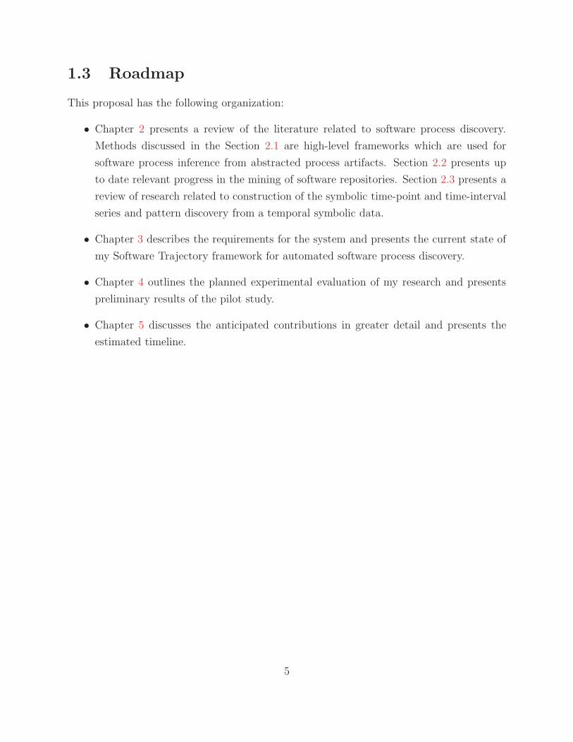
1.3 Roadmap
This proposal has the following organization:
• Chapter 2 presents a review of the literature related to software process discovery.
Methods discussed in the Section 2.1 are high-level frameworks which are used for
software process inference from abstracted process artifacts. Section 2.2 presents up
to date relevant progress in the mining of software repositories. Section 2.3 presents a
review of research related to construction of the symbolic time-point and time-interval
series and pattern discovery from a temporal symbolic data.
• Chapter 3 describes the requirements for the system and presents the current state of
my Software Trajectory framework for automated software process discovery.
• Chapter 4 outlines the planned experimental evaluation of my research and presents
preliminary results of the pilot study.
• Chapter 5 discusses the anticipated contributions in greater detail and presents the
estimated timeline.
5
Chapter 2
Related work
The purpose of this chapter is to review related work in software process discovery and
unsupervised temporal pattern mining. These two research areas provide a basis for my
research. I am planning to use unsupervised temporal pattern mining methods for the
automated discovery of recurrent behavioral patterns from the stream of low-level process
and product artifacts generated by the software process. These patterns, in turn, will be
used for software process discovery.
Discovery of recurrent behaviors in software process discussed in the Section 2.1. Min-
ing recurrent evolutionary patterns from software repositories discussed in the Section 2.2.
General algorithms of temporal data mining discussed in Section 2.3.
2.1 Software process discovery
Although process mining in the business domain is a well-established field with much software
developed up to date (ERP, WFM and other systems), “Business Process Intelligence” tools
usually do not perform process discovery and typically offer relatively simple analyses that
depend upon a correct a-priori process model [52] [3]. This fact restricts direct application
of business domain process mining techniques to software engineering, where processes are
usually performed concurrently by many agents, are more complex and typically have a
higher level of noise. Taking this fact in account, I will review only the approaches to the
mining for which applicability to software process mining was expressed.
Three papers are reviewed in this section:
• Cook & Wolf in [13] discuss an event-based framework for process discovery based on
grammar inference and finite state machines. The authors directly applied their frame-
6
work to Software Configuration Management (SCM) logs demonstrating satisfactory
results.
• Van der Aalst et al. [52] demonstrate the applicability of Transition Systems and
labeled Petri nets to process discovery in general. While this paper does not apply its
results directly to software process, the subsequent work by van der Aalst and Rubin
[45] discusses software process application.
• The third paper, by Jensen & Scacchi [23], while not presenting a pattern mining
strategy, describes an interesting framework built upon an universal generic meta-
model and specific to the observed processes models which are iteratively built and
revised during case studies. The value of this paper is in the demonstration of the
importance of the correct mapping between process artifacts and process entities as
well as a demonstration of iterative, human-involved technique of process revision which
is emphasizing importance of pre-existing domain knowledge in the effective pruning
of the search space.
As pointed by the authors in the reviewed papers, the proposed methods have difficulties
dealing with concurrency, which, in turn, is inevitable in the software process usually per-
formed by many agents. Much successive work has been done extending reviewed approaches
to the concurrent processes. Among others, Weijters & van der Aalst in [59] propose heuris-
tics to handle concurrency and noise issues, while van der Aalst et al. in [53] discuss a genetic
programming application.
2.1.1 Process discovery through Grammar Inference
Perhaps, the research most relevant to my own was done by Cook & Wolf in [13]. The authors
developed a “process discovery” techniques intended to discover process models from event
streams. The authors did not really intend to generate a complete model, but rather to
generate sub-models that express the most frequent patterns in the event stream. They
designed a framework which collects process data from ongoing software process or from
history logs, and generates a set of recurring patterns of behavior characterizing observed
process. In this work they extended two methods of grammar inference from previous work:
purely statistical (neural network based RNet) and purely algorithmic (KTail) as well as
developing their own Markovian method (Markov).
Process discovery, in the author’s opinion, resembles the process of grammar inference,
which can be defined as the process of inferring a language grammar from the given set
7
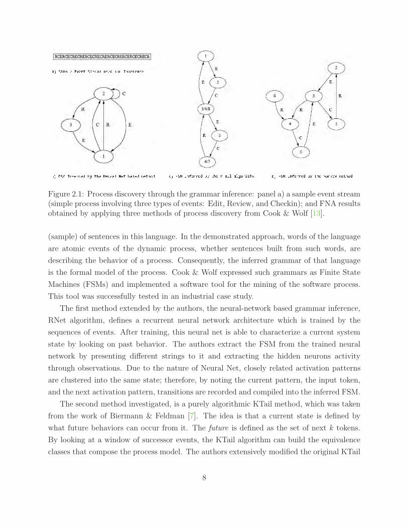
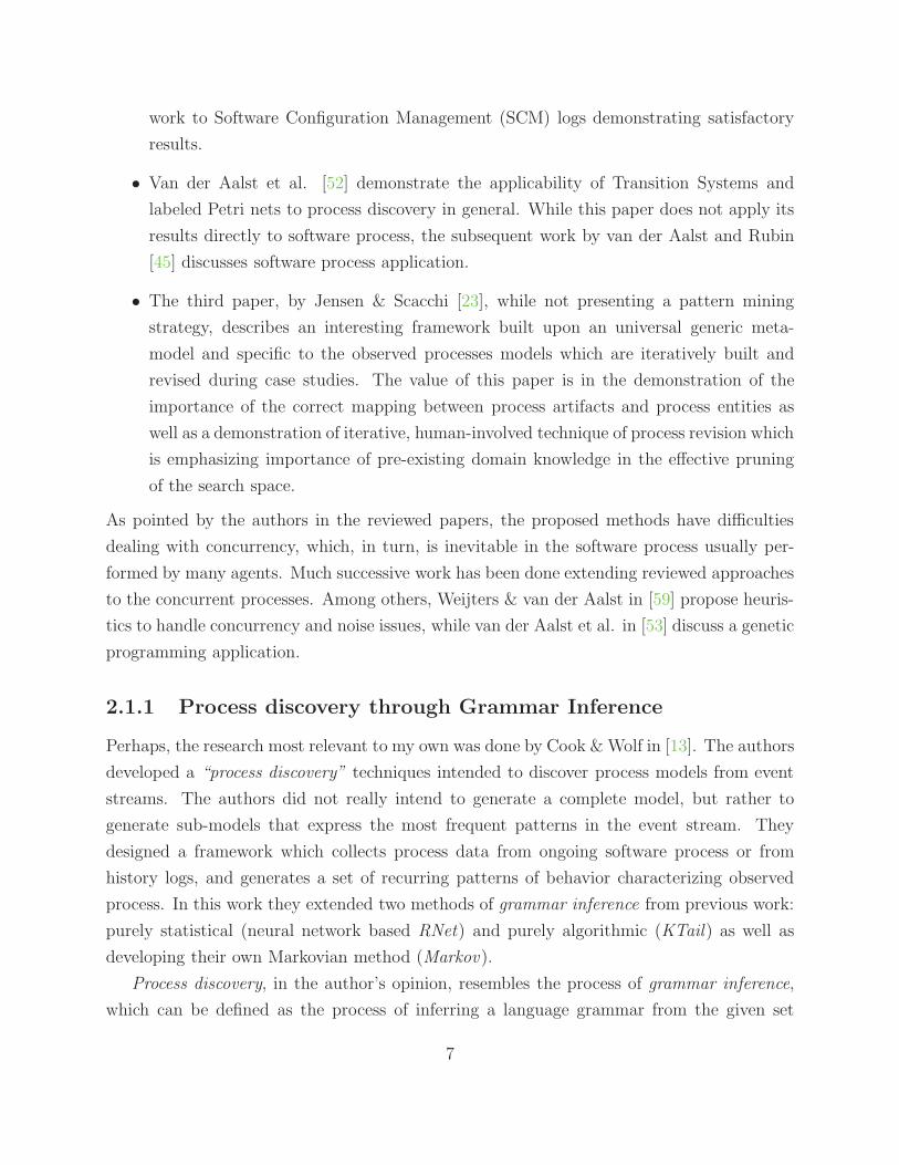
Figure 2.1: Process discovery through the grammar inference: panel a) a sample event stream(simple process involving three types of events: Edit, Review, and Checkin); and FNA resultsobtained by applying three methods of process discovery from Cook & Wolf [13].
(sample) of sentences in this language. In the demonstrated approach, words of the language
are atomic events of the dynamic process, whether sentences built from such words, are
describing the behavior of a process. Consequently, the inferred grammar of that language
is the formal model of the process. Cook & Wolf expressed such grammars as Finite State
Machines (FSMs) and implemented a software tool for the mining of the software process.
This tool was successfully tested in an industrial case study.
The first method extended by the authors, the neural-network based grammar inference,
RNet algorithm, defines a recurrent neural network architecture which is trained by the
sequences of events. After training, this neural net is able to characterize a current system
state by looking on past behavior. The authors extract the FSM from the trained neural
network by presenting different strings to it and extracting the hidden neurons activity
through observations. Due to the nature of Neural Net, closely related activation patterns
are clustered into the same state; therefore, by noting the current pattern, the input token,
and the next activation pattern, transitions are recorded and compiled into the inferred FSM.
The second method investigated, is a purely algorithmic KTail method, which was taken
from the work of Biermann & Feldman [7]. The idea is that a current state is defined by
what future behaviors can occur from it. The future is defined as the set of next k tokens.
By looking at a window of successor events, the KTail algorithm can build the equivalence
classes that compose the process model. The authors extensively modified the original KTail
8

algorithm improving the folding in the mined model making to make it more robust to noise.
The Markov based method developed by the authors is based on both algorithmic and
statistical approaches. It takes to account past and future system behavior in order to
guess the current system state. Assuming that a finite number of states can define the
process, and that the probability of the next state is based only on the current state (Markov
property), the authors built a nth-order Markov model using the first and second order
probabilities. Once built, the transition probability table corresponding to the Markov model
is converted into FSM which is in turn reduced based on the user-specified cut-off threshold
for probabilities.
The authors implemented all three of these algorithms in a software tool called DaGama
as a plugin for larger software system called Balboa [11]. By performing benchmarking, Cook
& Wolf found that the Markov algorithm was superior to the two others. RNet was found
to be the worst of the three algorithms.
Overall, while having some issues with the complexity of produced output and noise han-
dling, the authors proved applicability of implemented algorithms to real-world process data
by demonstrating an abstraction of the actual process executions and capturing important
properties of the process behavior. The major backdraw of the approach, as stated by the
authors, lies in the inability of the FSMs to model concurrency of processes which limits its
applicability to the software development process. Later, Cook et al. in [12] addressed this
limitation.
2.1.2 Incremental Workflow Mining with Petri Nets
Another set of findings relevant to my research approach was developed by Rubin et al.
[45] and van der Aalst et al. [52] and is called incremental workflow mining. The authors
not only designed sophisticated algorithms but built a software system using a business
process mining framework called ProM by van Dongen et al. [54] which synthesizes a Petri
Net corresponding to the observed process. The system was tested on SCM logs and while
the process artifacts retrieved from the SCM system are rather high-level, the approach
discussed is very promising for the modeling of software processes from the low-level product
and process data.
Within the incremental workflow mining framework, the input data from the SCM audit
trail information is mapped to the event chain which corresponds to the software process
artifacts. The authors call this process abstraction on the log level which is implemented as
a set of filters which not only aggregates basic events into single high-level entities but also
9

Figure 2.2: Illustration of the “Generation and Synthesis Approach” from [54]: a) TransitionSystem with regions shown; b),c) Petri Nets synthesized from the Transition System.
removes data irrelevant to the mining process (noise).
The event chain constructed through the abstraction is then treated with the Generate
part of the “Generate and Synthesis” [52] algorithm in order to generate a Transition System
which represents an ordered series of events. This algorithm looks at the history (prefix)
and the future (suffix) sequences of events related to the current one in order to discover
transitions. When applied to the abstracted log information, the algorithm generates a rather
large Transition System graph where edges connect to abstracted events. This transition
system is then successively simplified by using various reduction strategies such as “Kill
Loops”, “Extend”, “Merge by Output” and others; it is possible to combine these reduction
strategies in order to achieve a greater simplification.
At the last step of the incremental workflow mining approach, Transition Systems are
used to Synthesize labeled Petri nets (where different transition can refer to the same event)
with the help of “regions theory” [14]. As with the Transition System generation, the authors
investigate many different strategies of Petri nets synthesis, showing significant variability
in the results achieved. (see Figure 2.2).
The significant contribution of this research is in the generality of the method. It was
shown that by tuning the “Generate” and “Synthesize” phases it is possible to tailor the
algorithm to a wide variety of processes. In particular, as mentioned before, Rubin et al.
successfully applied this framework to the SCM logs analysis.
10

Figure 2.3: Example of the reference model mapping from [23].
2.1.3 Reference model for Open Source Software Processes Dis-
covery
Jensen & Scacchi in [23] take a somewhat different approach from the previously discussed
research efforts. The authors are follow a top-down approach and do not try to build a
software process model from available process artifacts. Instead, they try to develop a
software process reference model by iteratively refining mapping between observed artifacts
and the model entities.
The proposed software process reference model is a layer which provides a mapping
from the underlying recognized software process artifacts into a higher level software-process
meta-model by Mi & Sacchi [40]. The iterative revision of the reference model vocabulary
of mapped terms (Figure 2.3) is performed through case studies. During such a study, the
observed process artifacts such as SCM logs, defect reports and others are queried with terms
from the reference model pulling correlated artifacts which are revised and curated by the
process expert and lead to the further revisions of the terms taxonomy on the next iteration.
In the relation to my research, I am envisioning the application of such iterative “meta-
model driven approach” for characterization of the discovered recurrent patterns with un-
known generative phenomena. The creation of the low-level recurrent patterns taxonomy
through successive mapping into the meta-model assures from a “nonsense patterns” discov-
ery.
2.2 Mining software repositories
According to Kagdi et al. [27] the term mining software repositories (MSR) “... has been
coined to describe a broad class of investigations into the examination of software reposito-
ries.” The “software repositories” here refer to various sources containing artifacts produced
11

by software process. Examples of such sources are version-control systems (CVS, SVN, etc.),
requirements/change/bug control systems (Bugzilla, Trac etc.), mailing lists archives and so-
cial networks. These repositories have different purposes but they support a single goal - a
software change which is the single unit of the software evolution.
In the literature, software change defined as an addition, deletion or modification of any
software artifact such as requirement, design document, test case, function in the source code,
etc. Typically, software change is realized as the source code modification; and while version
control system keeps track of actual source code changes, other repositories track various
artifacts (called metadata) about these changes: a description of a rationale behind a change,
tracking number assigned to a change, assignment to a particular developer, communications
among developers about a change, etc.
Researchers mine this wealth of data from repositories in order to extract relevant in-
formation and discover relationships about a particular evolutionary characteristic. For
example, one may be interested in the growth of a system during each change, or reuse of
components from version to version. In this section I will review some MSR research liter-
ature which is relevant to my research and based on the mining of temporal patterns from
SCM audit trails.
2.2.1 Mining evolutionary coupling and changes
One of the approaches in MSR mining relevant to my research is built upon mining of the
simultaneous changes occurring in software evolution. This type of mining considers changes
in the code within a short time-window interval which occur recurrently. Such changes are
revealing logical coupling within the code which can not be captured by the static code
analysis tools. This knowledge allows researcher and analysts predict the required effort and
impact of changes with a higher precision.
Mining of evolutionary coupling is typically performed on different levels of code abstrac-
tion: Zimmermann et al. in [64] discuss mining of version archives on the level of the lines of
source-code using annotation graphs; Ying et al. in [62] discuss mining of version archives for
co-change patterns among files by employing association rule mining algorithm, and refining
results by introducing interestingness measure, which based on the call and usage patterns
along with inheritance; Gall et al. in [51] use a window-based heuristics on CVS logs for
uncovering logical couplings and change patterns on the module/package level. Kim et al. in
[33] taking a different approach by mining function signature change and introducing kinds
of signature changes and its metrics in order to understand and predict future evolution
12

patterns and aid software evolution analysis.
The fine-grain mining of changes on the level of lines of source code is usually implemented
with the use of diff utilities family which report differences between versions of the same file.
For capturing temporal properties the sliding-window approach is used if mining CVS logs,
while Subversion is able to report co-changed filesets (change-sets). Use of the information
extracted by parsing issue/bug tracking logs and developer comments from version control
logs allows to capture co-occurring changes with higher precision.
What is common among all this work is that while researchers use different sources
and abstraction levels of information, they are extracting only the relevant to a specific
question data (using filters and taxonomy mappings) and compose data sets suitable for
KDD algorithms. In order to refine and classify (prune) reported results, various support
functions proposed.
The main contribution of this type of mining is in the discovery of patterns in software
changes which are improving our understanding of the software and allowing estimation of
effort and impact of new changes with higher precision.
2.2.2 Ordered change patterns
A step ahead in the analysis of co-occurring changes in source code entities was shown by
Kagdi et al. in [28]. The authors investigated a problem of mining ordered sequences of
changed files from change-sets. Six heuristics (Day, Author, File, Author-date, Author-file,
and Day-file) based on the version control transaction properties were developed and imple-
mented. Abstracted sequences were mined with Apriori algorithm (see 2.3.10) discovering
recurrent sequential patterns. The authors proposed a higher specificity and effectiveness of
such approach to software change prediction than by using convenient (un-ordered) change
patterns mining.
2.2.3 Usage patterns
Another interesting approach for MSR, relevant to my work, is the mining of usage patterns
proposed by Livshits & Zimmermann in [38]. In this work, the authors approach a problem
of finding violations of application-specific coding rules which are ultimately responsible for a
number of errors. They designed approach to find “surprise patterns” (see Subsection 2.3.7)
of the API and function usage in SCM audit trail by implementing a preprocessing of the
functional calls and mining aggregated data with a customized Apriori algorithm (see 2.3.10)
13
implementation. By considering past changes and bug fixes, authors were able to classify
patterns into three categories: valid patterns, likely error patterns, and unlikely patterns.
Candidate patterns found with Apriori algorithms were considered to be a valid pattern if
they were found a specified number of times and an unlikely patterns otherwise. Similarly,
if a previously labeled as valid pattern was later violated a certain number of times, it was
considered as an error pattern. The authors validated their approach on mining publicly
available repositories effectively reporting error patterns.
2.3 Temporal data mining
My research in software process discovery mainly rests on the mining of recurrent behavioral
patterns from a representation of software processes as a temporal sequences of events per-
formed by individual developers or automated tools with or without concurrency. As we saw
in the previous sections of this Chapter, it is possible not only to infer the known high-level
processes from observing low-level artifacts, but also to discover novel processes through the
use of a unsupervised process mining techniques.
In my research, the collection of development artifacts is performed by Hackystat, a
framework for automated software process and product metrics collection and analysis. The
event streams provided by Hackystat are very rich in information. They provide temporal
data about atomic events, such as invoking of a build tool or performing a test, along with
a great variety of process and product metrics such as cyclomatic complexity of the code, or
amount of effort applied to software development and many other. It is possible to retrieve
other very low-level artifacts such as buffer transfers within the IDE editor or background
compilation activities. All of these artifacts characterize the dynamic behavior of a software
process in great detail.
In order to perform analyses in my system, I am extracting the necessary process data
with a desired granularity from the Hackystat and converting it into a symbolic representa-
tion by performing a direct mapping based on the taxonomy of events or by approximating
telemetry streams (time-series) with Piecewise Aggregate Approximation (section 2.3.1) and
Symbolic Aggregate approXimation (section 2.3.2). This symbolic representation of the ob-
served software processes are used in the Software Trajectory analyses which build upon
Symbolic Temporal Data Models (section 2.3.4), Temporal Concepts (section 2.3.3) and
Temporal Operators (section 2.3.6).
Section 2.3.7 defines temporal patterns of motif and surprise along with discussing rel-
14

evant pattern search algorithms and data structures used for the indexing. Section 2.3.10
presents AprioriAll algorithm for unsupervised pattern mining.
2.3.1 Piecewise Aggregate Approximation (PAA)
According to Yi & Faloutsos [61], most of the prior research in the time series indexing was
centered around the Euclidean distance (L2) applied to time sequences, where the method
proposed by the authors enable efficient multi-modal similarity search. Supporting the claim,
the authors explain some of pitfalls of previously published spectral-decomposition methods
such as DFT, DCT, SVD etc. whose core algorithm employs Euclidean distance based
metrics over a set of transform coefficients is shown to be inefficient over other distance
functions.
The proposed method performs a time-series feature extraction based on segmented
means. Given a time-series X of length n transformed into vector X = (x1, ..., xM) of
any arbitrary length M ≤ n where each of xi is calculated by the following formula:
xi =M
n
(n/M)i∑j=n/M(i−1)+1
xj (2.3.1.1)
This simply means that in order to reduce the dimensionality from n to M , we first divide
the original time-series into M equally sized frames and secondly compute the mean values
for each frame. The sequence assembled from the mean values is the PAA transform of the
original time-series. It was shown by Keogh et al. that the complexity of the PAA transform
can be reduced from O(NM) (2.3.1.1) to O(Mm) where m is the number of sliding windows
(frames). The satisfaction of the transform to a bounding condition in order to guarantee
no false dismissals was also shown by Yi & Faloutsos for any Lp norms and by Keogh et al.
[30] by introducing the distance function:
DPAA(X, Y ) ≡√
n
M
√√√√ M∑i=1
(xi − yi) (2.3.1.2)
and showing that DPAA(X, Y ) ≤ D(X, Y ).
15

Figure 2.4: The illustration of the SAX approach taken from [37] depicts two pre-determinedbreakpoints for the three-symbols alphabet and the conversion of the time-series of lengthn = 128 into PAA representation followed by mapping of the PAA coefficients into SAXsymbols with w = 8 and a = 3 resulting in the string baabccbc.
2.3.2 Symbolic Aggregate approXimation (SAX)
Symbolic Aggregate approXimation was proposed by Lin et al. in [37]. This method ex-
tends the PAA-based approach, inheriting algorithmic simplicity and low computational
complexity, while providing satisfiable sensitivity and selectivity in range-query processing.
Moreover, the use of a symbolic representation opens the door to the existing wealth of data-
structures and string-manipulation algorithms in computer science such as hashing, regular
expression pattern matching, suffix trees etc.
SAX transforms a time-series X of length n into a string of arbitrary length ω, where
ω << n typically, using an alphabet A of size a ≥ 2. The SAX algorithm consist of two steps:
during the first step it transforms the original time-series into a PAA representation and this
intermediate representation gets converted into a string during the second step. Use of
PAA at the first step brings the advantage of a simple and efficient dimensionality reduction
while providing the important lower bounding property as shown in the previous section.
The second step, actual conversion of PAA coefficients into letters, is also computationally
efficient and the contractive property of symbolic distance was proven by Lin et al. in [36].
Discretization of the PAA representation of a time-series into SAX is implemented in a
way which produces symbols corresponding to the time-series features with equal probability.
The extensive and rigorous analysis of various time-series datasets available to the authors
has shown that normalized by the zero mean and unit of energy time-series follow the Normal
distribution law. By using Gaussian distribution properties, it’s easy to pick a equal-sized
areas under the Normal curve using lookup tables [35] for the cut lines coordinates, slicing
the under-the-Gaussian-curve area. The x coordinates of these lines called “breakpoints” in
16

Figure 2.5: The visual representation of the two time-series Q and C and three distancesbetween their representation: Euclidean distance between raw time-series (A), the distancedefined for PAA coefficients (B) and the distance between two SAX representations (C).(The figure taken from [37] as well)
the SAX algorithm context. The list of breakpoints B = β1, β2, ..., βa−1 such that βi−1 < βi
and β0 = −∞, βa = ∞ divides the area under N(0, 1) into a equal areas. By assigning a
corresponding alphabet symbol alphaj to each interval [βj−1, βj), the conversion of the vector
of PAA coefficients C into the string C implemented as follows:
ci = alphaj , iif ci ∈ [βj−1, βj) (2.3.2.1)
SAX introduces new metrics for measuring distance between strings by extending Eu-
clidean and PAA (2.3.1.2) distances. The function returning the minimal distance between
two string representations of original time series Q and C is defined as
MINDIST (Q, C) ≡√
n
w
√√√√ w∑i=1
(dist(qi, ci))2 (2.3.2.2)
where the dist function is implemented by using the lookup table for the particular set of
the breakpoints (alphabet size) as shown in Table 2.1, and where the singular value for each
cell (r, c) is computed as
cell(r,c) =
⎧⎨⎩
0, if |r − c| ≤ 1
βmax(r,c)−1 − βmin(r,c)−1, otherwise(2.3.2.3)
17

a b c da 0 0 0.67 1.34b 0 0 0 0.67c 0.67 0 0 0d 1.34 0.67 0 0
Table 2.1: A lookup table used by the MINDIST function for the a = 4
As shown by Li et al., this SAX distance metrics lower-bounds the PAA distance, i.e.
n∑i=1
(qi − ci)2 ≥ n(Q − C)2 ≥ n(dist(Q, C))2 (2.3.2.4)
The SAX lower bound was examined by Ding et al. [16] in great detail and found to be
superior in precision to the spectral decomposition methods on bursty (non-periodic) data
sets.
2.3.3 Symbolic series, temporal models, concepts, and operators
The SAX transformation procedure described in the previous section yields symbolic time-
series based on the real-valued data. Having such a symbolic representation (also called in
the literature a symbolic temporal data) is very advantageous compared to the real-valued
data due to the many algorithms available for the string processing. Moreover, having
homogeneous symbolic series corresponding to low-level process artifacts combined with the
symbolic event streams from the SCM or bug tracking system creates a rich data field for
in-depth software process analysis. In following subsections I will review symbolic temporal
data models, temporal concepts and operators.
2.3.4 Temporal data models
Morchen aggregates much work in the field of data mining from symbolic temporal data in
[41]. Two figures taken from this report (Figure 2.6) depict a hierarchy of time-points (left
panel) and time-intervals (right panel) data models, concepts and operators.
While the time-points data model is intuitive and resembles the actual real-valued time
series, the time-intervals temporal data model is built upon the concept of duration which is
a repetition of the property over several time-points. Time-intervals are continuous groups
of discrete time instants and some of the algorithms and applications operate with this
18
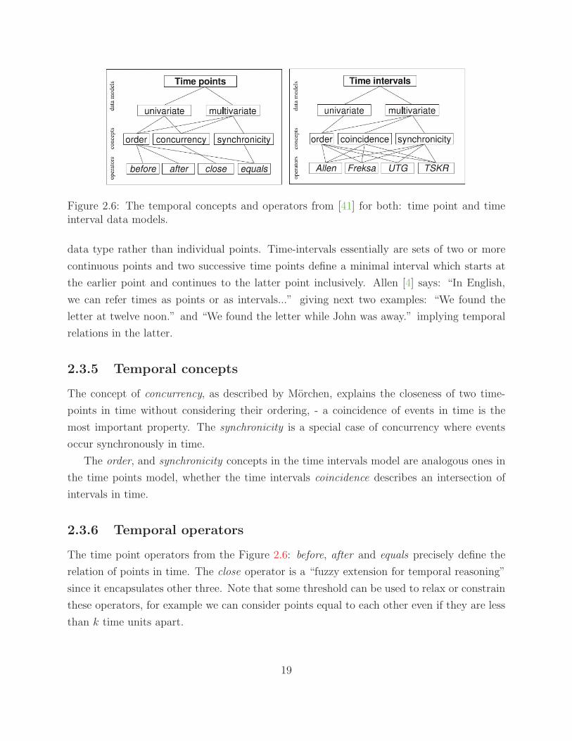
Figure 2.6: The temporal concepts and operators from [41] for both: time point and timeinterval data models.
data type rather than individual points. Time-intervals essentially are sets of two or more
continuous points and two successive time points define a minimal interval which starts at
the earlier point and continues to the latter point inclusively. Allen [4] says: “In English,
we can refer times as points or as intervals...” giving next two examples: “We found the
letter at twelve noon.” and “We found the letter while John was away.” implying temporal
relations in the latter.
2.3.5 Temporal concepts
The concept of concurrency, as described by Morchen, explains the closeness of two time-
points in time without considering their ordering, - a coincidence of events in time is the
most important property. The synchronicity is a special case of concurrency where events
occur synchronously in time.
The order, and synchronicity concepts in the time intervals model are analogous ones in
the time points model, whether the time intervals coincidence describes an intersection of
intervals in time.
2.3.6 Temporal operators
The time point operators from the Figure 2.6: before, after and equals precisely define the
relation of points in time. The close operator is a “fuzzy extension for temporal reasoning”
since it encapsulates other three. Note that some threshold can be used to relax or constrain
these operators, for example we can consider points equal to each other even if they are less
than k time units apart.
19
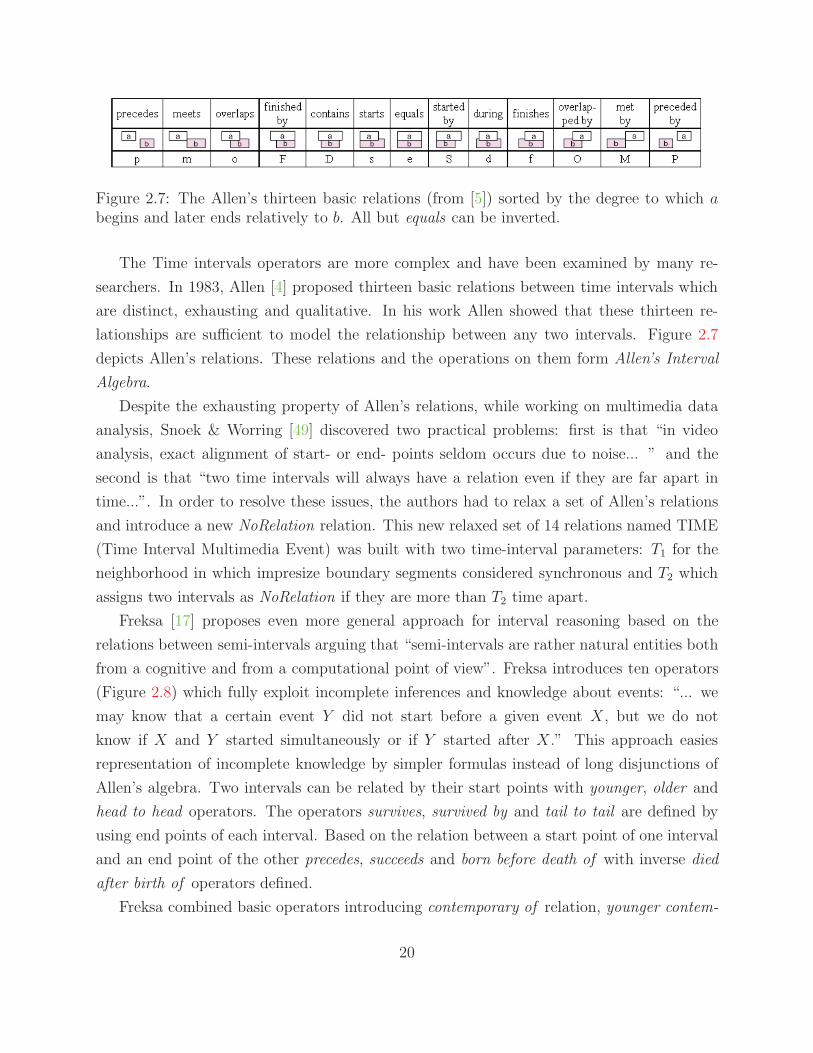
Figure 2.7: The Allen’s thirteen basic relations (from [5]) sorted by the degree to which abegins and later ends relatively to b. All but equals can be inverted.
The Time intervals operators are more complex and have been examined by many re-
searchers. In 1983, Allen [4] proposed thirteen basic relations between time intervals which
are distinct, exhausting and qualitative. In his work Allen showed that these thirteen re-
lationships are sufficient to model the relationship between any two intervals. Figure 2.7
depicts Allen’s relations. These relations and the operations on them form Allen’s Interval
Algebra.
Despite the exhausting property of Allen’s relations, while working on multimedia data
analysis, Snoek & Worring [49] discovered two practical problems: first is that “in video
analysis, exact alignment of start- or end- points seldom occurs due to noise... ” and the
second is that “two time intervals will always have a relation even if they are far apart in
time...”. In order to resolve these issues, the authors had to relax a set of Allen’s relations
and introduce a new NoRelation relation. This new relaxed set of 14 relations named TIME
(Time Interval Multimedia Event) was built with two time-interval parameters: T1 for the
neighborhood in which impresize boundary segments considered synchronous and T2 which
assigns two intervals as NoRelation if they are more than T2 time apart.
Freksa [17] proposes even more general approach for interval reasoning based on the
relations between semi-intervals arguing that “semi-intervals are rather natural entities both
from a cognitive and from a computational point of view”. Freksa introduces ten operators
(Figure 2.8) which fully exploit incomplete inferences and knowledge about events: “... we
may know that a certain event Y did not start before a given event X, but we do not
know if X and Y started simultaneously or if Y started after X.” This approach easies
representation of incomplete knowledge by simpler formulas instead of long disjunctions of
Allen’s algebra. Two intervals can be related by their start points with younger, older and
head to head operators. The operators survives, survived by and tail to tail are defined by
using end points of each interval. Based on the relation between a start point of one interval
and an end point of the other precedes, succeeds and born before death of with inverse died
after birth of operators defined.
Freksa combined basic operators introducing contemporary of relation, younger contem-
20

Figure 2.8: Panel a): Freksas semi-interval relations between the intervals A and B withinverse operators in italics. Panels b), c), d): Alternative interval operators.
porary of, older contemporary of, surviving contemporary of, survived by contemporary of,
older & survived by and younger & survives.
Rainsford & Roddick in [44] implemented a system of temporal knowledge discovery based
on the Freksa’s relations. Later, Roddick introduced Midpoint Interval Operators extending
Allen’s and Vilain’s five-points [55] relations with nine different overlaps. Two overlaps large
overlap and small overlap depicted at the Figure 2.8 panel b. This improvement allowed the
handling of coarse temporal data and data from streams.
Further extensions were proposed by Morchen & Ultsch in the form of UTG (Unification-
Based Temporal Grammar) introducing an extension to the Allen’s equals operator with
more or less simultaneous and coincides operators as shown at the Figure 2.8 panels c
and d. Later, the Time Series Knowledge Representation (TSKR) hierarchical language for
expressing temporal knowledge in time interval data was built by the same authors on the
base of UTG [42]. It was shown that TSKR, while compared to other alternative approaches,
has advantages in robustness, expressivity, and comprehensibility
2.3.7 Temporal patterns and indexing
In previous sections of this chapter I have shown the PAA and SAX algorithms for conversion
of real valued time series into the symbolic representation along with symbolic temporal
data models, concepts and operators. All of this is a necessary background in order to
21

understand approaches for unsupervised knowledge mining from a symbolic temporal data.
In this section I will review sequential pattern mining algorithms from time points and time-
intervals data. I will begin the review by focusing on the univariate data and then extend it
to the multivariate.
Before discussing algorithms, I need to provide a formal definition of pattern. The es-
sential property which defines a pattern is called support. Support, roughly speaking, is the
frequency of occurrence of a certain pattern in the observed data. It is generally assumed
that each of the possible patterns have a certain probability to be seen in the dataset just
by chance, and this probability is called the expected probability and defines the expected
support for the pattern. When the actual observed support (or frequency) of a pattern sig-
nificantly differs from the expected one, it is called significant support and indicates that
pattern might have some meaningful knowledge artifact attached to it. Although support
different from the expected level does not guarantee usefulness or interestingness, it is used
for a powerful pruning of a search space since most possible patterns will not have sufficient
support. Note that there is property [56] discussed in the literature which essentially similar
to support: confidence. Usually confidence correlates with support, i.e. greater support
corresponds to higher confidence.
There are two well-established categories of patterns with significant support. The first
category of patterns, frequently occurring ones (with support higher than expected), is very
important in many data mining areas such as medicine, motion-capture, robotics, video
surveillance, meteorology and others. Patterns from this category usually named as repeated,
approximately repeated or motifs. The second category of patterns, contains patterns with
the support lower than expected, this type of pattern is named surprise or novelty patterns.
Novelty patterns also have a great value for many applications: for example it is important to
detect unusual semi-repeated pattern in the ECG data diagnosing heartbeat abnormalities,
or detecting unusual activity patterns in video surveillance recognizing a suspicious activity.
The temporal motif finding problem from symbolic data is very similar to one of the
central problems in the field of Computational Biology [26]. Many algorithms are very
similar, but, in Biology, motifs are usually informative and bear some information about
evolutionary artifacts, which is not true in the field of time-series analysis [60].
2.3.8 Time points patterns
According to Morchen, the most commonly searched pattern within univariate symbolic time
series is order. This search for a particular order of symbols within a subsequence is called
22

Figure 2.9: The time-points patterns as explained in [41]
sequential pattern mining [2] and does not necessarily require symbols to be consecutive.
The classical suffix tree algorithm [50] with some modifications is a standard approach
for pattern discovery from string time-series according to Palopoli et al. [43]. In this paper,
the authors discuss algorithms for automatic discovery of frequent patterns (motifs) in “ex-
act” or “approximate” forms. There are two approaches generally used for the suffix tree
building: generative, when algorithms generate all possible patterns and test their appear-
ance frequency [57], and scanning, when a sliding window used to scan over the sequences
available and construct the tree on the fly [57]. In [24] Jiang & Hamilton compare traversal
strategies for suffix trees: breadth-first (BF , O(K2n)), depth-first (DF , O(Kn)) and the
heuristic depth-first (HDF) algorithms implementations for temporal data mining.
The limitation of the suffix-tree based algorithms is that the maximum length of a pat-
tern needs to be specified upon tree construction since all sub-sequences of this length are
generated or extracted from the time series with a sliding window.
Another approach, specifically designed for the surprise pattern finding problem, is pro-
posed by Keogh et al. in [32]. The authors discuss methods for finding a surprise pattern
from the temporal data and propose their “TARZAN” algorithm which is based upon suffix
tree and Markov model, reporting surprising patterns occurring with a frequency substan-
tially different from that expected by chance.
2.3.9 Time interval patterns
As we saw before, the duration concept is implicit in the time interval definition. Neverthe-
less, while defining a time-interval pattern we do not actually take into account the length
23

Figure 2.10: The time-interval patterns from [41]
of the interval. Interval relations are abstracted to the “border” or “mean points” relations.
Containment patterns are discussed by Villafane et al. in [56]. This type of temporal
patterns has found application to many areas, for example software system log mining. In
this case it is important to see what events were happening within the resource overload time
interval. Another example is medicine: what was happening with the heartbeat within the
period when patient’s fever was high? The authors propose a method based on containment
graphs which allows counting of the containment frequency based on a lattice. The authors
designed a naive algorithm of the graph traversal performed incrementally by the path-
size and have shown satisfiable results considering their limitations in computational power.
One of the limitations found is that it yields different patterns describing the same temporal
events. An example of containment patterns is shown at Figure 2.10 panel a, this figure is
borrowed from [41].
Allen’s relations are used in many of the approaches to mining of time-interval patterns.
In [29], Kam & Fu considered interval-based events where duration is expressed in terms
of end-points relations and designed a category of A1 temporal patterns based on Allen’s
relations. However, Kam and Fu restrict the search space to the right concatenations of
intervals corresponding to existing patterns and limit the depth of the patterns. Depending
on time-interval consideration order, this approach yields different patterns describing same
events, for example on the Figure 2.10 panel b: left pattern is (((A starts B) overlaps C)
overlaps D) whether right one is (((A before C) started by B) overlaps D).
24

Fluents, another type of time-interval patterns based on the Allen’s algebra, were intro-
duced by Cohen in [9] to address the problem of unsupervised learning of structures in time
series. The formal definition given by the authors states that “Fluents are logical descrip-
tions of situations that persist, and composite fluents are statistically significant temporal
relationships between fluents.” Sliding window and Apriori algorithms are used in this work.
The Fluent learning algorithm designed by the authors was applied to the robot motion data
collected by sensors and helped in the discovery of temporal patterns indicating persistent
robot behavior along with problems with robot’s sonar system. This algorithm suffers from
the same problem as A1 - it reports variations of the same pattern as different patterns. The
authors had to remove “the set of variants” manually before presenting results.
Hoppner, in [22], demonstrates an approach to association rules mining through the use
of state sequences. State sequences based on pairwise relations between all temporal intervals
according to Allen. A sliding window is used to generate sub-sequences and the duration
of the pattern over consecutive sliding windows is used to quantify the pattern support
value. This information is then used in the Apriori algorithm for pattern discovery. The
experimental validation of the algorithm on the weather dataset shows the ability of the
approach to yield meaningful patterns.
UTG relations were used in some work for temporal interval patterns mining (Figure
2.10 panel d), but according to Morchen [41], it was “criticized for the strict conditions
relating interval boundaries”. UTG rules place restrictions on the intervals, requiring the
start and end of the intervals in the pattern to be almost simultaneous. Also, lacking the
ability to express the concept of coincidence, UTG-based methods found somewhat limited
application. However, Guimaraes in [20] shows targeted application of UTG-based linguistic
knowledge representation to the discovery of sleep-related breathing disorders. Results of this
study allowed doctors to improve diagnosis, and moreover, led to the discovery of previously
unknown recurrent behaviors among patients.
Unlike UTG, TSKRpatterns provide support for a partial order and allow inclusion of
the sub-intervals into the pattern. This makes them more expressive than UTG and Allen’s
relations. TSKR Chord patterns shown at the Figure 2.10 panel e are mined with the
CHARM [63] algorithm extended with a support function that counts the duration of the
pattern occurrence [41]. TSKR Phrase patterns, in turn, are built upon the partial order of
the several Chords (2.10 panel f ), and provide greater sensitivity and selectivity for temporal
patterns mining.
25

Large 3-sequences Candidate 4-sequences Candidate 4-sequencesafter join after pruning
{1, 2, 3} {1, 2, 3, 4} {1, 2, 3, 4}{1, 2, 4} {1, 2, 4, 3}{1, 3, 4} {1, 3, 4, 5}{1, 3, 5} {1, 3, 5, 4}{2, 3, 4}
Table 2.2: Illustration of AprioriAll algorithm generative function by Agrawal & Srikant [2].4-sequences candidates are generated from 3-sequences by join and pruned in turn.
2.3.10 Apriori algorithm
I have mentioned several applications of the Apriori algorithm while reviewing temporal
patterns mining from symbolic time-points and time-interval series. The family of Apriori
algorithms was proposed in 1995 by Agrawal & Srikant [2]. These algorithms are based on
the naive apriori association rule stating that any sub-pattern of a frequent pattern must be
frequent.
The authors has shown application of their algorithms to the mining of recurrent behavior
patterns from a database of purchase transactions. They used a support function which is
defined as the fraction of the customers supporting such a pattern. The problem solved in
this work with the Apriori algorithm can be stated formally: “given a database of customer
transactions, find the set of maximal sequences among all others that have at least user-
specified support”.
The naive Apriori algorithm starts by building a set of maximal sequences by finding all
“candidate” patterns of size 1 with a support value that is greater or equal to the specified
minimum. On the next step, the algorithm generates a successive set of candidate patterns
by extending each of the candidate patterns by 1, and testing it against the database for
sufficient support. The algorithm iterates over this second step, until it terminates when no
further extension is possible, yielding a set of maximal sequences. While being simple, and
proven to produce a correct solution, the naive approach is extremely inefficient due to the
high time cost of the database scanning phase (which is the product of an amount of time
needed for a single pass over the database and the number of generated candidates).
The significant improvement of the generative function and the scanning speed over the
naive approach is the main contribution of Agrawal & Srikant. First, they designed a clever
generative function which efficiently prunes the search space by excluding non-existing se-
26
quences of length n + 1 just by looking at the existing set on sequences of length n. Second,
the authors’ implementation of the database scanning leverages the use of efficient inter-
mediate in-memory index (built with a hash-tree and conducts breadth-first search). is to
transform (shrink) the database of transactions during each step. During this transforma-
tion each of the individual transactions within single sequence is replaced by the “set of all
litemsets contained in that transaction. If a transaction does not contain any litemset, it is
not retained in the transformed sequence.” The “litemset” here refers to the item set with
a minimum support.
AprioriAll, AprioriSome and DynamicSome by Agrawal & Srikant were the very first
algorithms for sequential pattern mining built upon the Apriori principle. While being far
more efficient than a naive implementation, they still require many passes over the database
while testing candidate sequences. Many other algorithms based on this implementation
were proposed. In 1996 Srikant & Agrawal extended their original work with GSP (General-
ized Sequential Pattern) algorithm. GSP allows time constraints and relaxes the definition
of transaction; additional improvement was achieved by use of the knowledge of taxonomies
which prunes search space by excluding non-interesting sequences. Wang et al. in 2001 pro-
posed a GSP-based MFS (Mining Frequent Sequences) [58] algorithm based on the concept
of pre-large sequences which further reduces the amount of rescanning.
27

Chapter 3
Software Trajectory: a software
process mining framework.
As we saw in Chapter 2, it is possible to infer and successively formalize software process
by observing its artifacts, and in particular, recurrent behavioral patterns. The problem of
finding such patterns is the cornerstone of my research. My approach to this problem rests
on the application of data-mining techniques to symbolic time-point and time-interval series
constructed directly from the real-valued telemetry streams provided by Hackystat.
To investigate the requirements for a software tool that aids in the discovery of recur-
rent behavioral patterns in software process, I am designing and developing the “Software
Trajectory” framework. A high-level overview of the framework is shown in Figure 3.1 and
resembles the flow of the “Knowledge Discovery in Database” process discussed by Han et
al. in [21]. As shown, the data collected by Hackystat is transformed into a symbolic format
and then indexed for further use in data-mining. The tools, designed for data-mining, have
a specific restrictions placed on the search space by domain and context knowledge in an
attempt to limit the amount of reported patterns to useful ones. I am planning to design a
GUI in a way that will allow easy access and modification of these restrictions.
3.1 Current state of development
I started development of the Software Trajectory framework in early 2008 by designing
a user interface for visual comparison of multi-variate time series. I called this package
“TrajectoryBrowser” and called its results “Software Trajectory Analysis”. The idea was
to visualize software project metrics as a set of trajectories in 3D space, as opposed to the
28
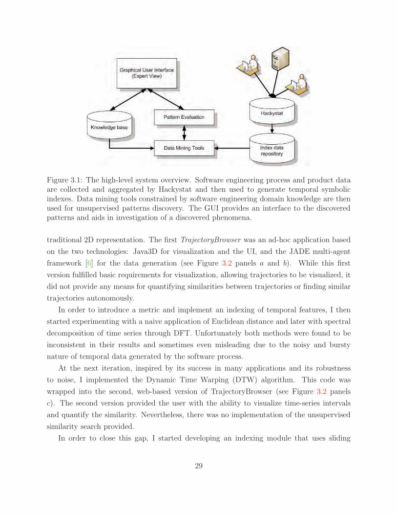
Figure 3.1: The high-level system overview. Software engineering process and product dataare collected and aggregated by Hackystat and then used to generate temporal symbolicindexes. Data mining tools constrained by software engineering domain knowledge are thenused for unsupervised patterns discovery. The GUI provides an interface to the discoveredpatterns and aids in investigation of a discovered phenomena.
traditional 2D representation. The first TrajectoryBrowser was an ad-hoc application based
on the two technologies: Java3D for visualization and the UI, and the JADE multi-agent
framework [6] for the data generation (see Figure 3.2 panels a and b). While this first
version fulfilled basic requirements for visualization, allowing trajectories to be visualized, it
did not provide any means for quantifying similarities between trajectories or finding similar
trajectories autonomously.
In order to introduce a metric and implement an indexing of temporal features, I then
started experimenting with a naive application of Euclidean distance and later with spectral
decomposition of time series through DFT. Unfortunately both methods were found to be
inconsistent in their results and sometimes even misleading due to the noisy and bursty
nature of temporal data generated by the software process.
At the next iteration, inspired by its success in many applications and its robustness
to noise, I implemented the Dynamic Time Warping (DTW) algorithm. This code was
wrapped into the second, web-based version of TrajectoryBrowser (see Figure 3.2 panels
c). The second version provided the user with the ability to visualize time-series intervals
and quantify the similarity. Nevertheless, there was no implementation of the unsupervised
similarity search provided.
In order to close this gap, I started developing an indexing module that uses sliding
29
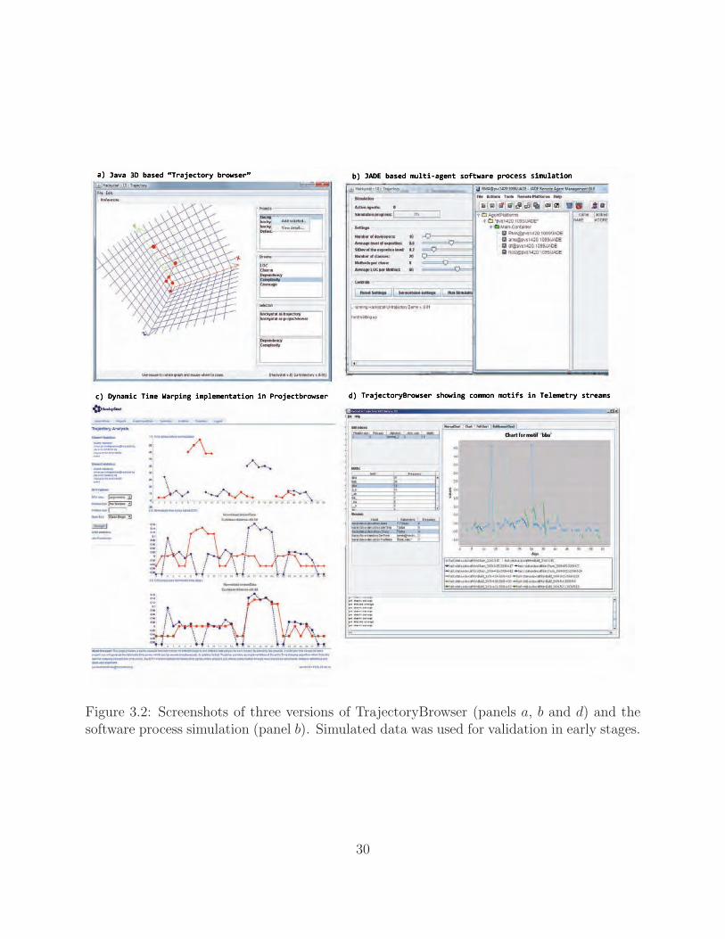
Figure 3.2: Screenshots of three versions of TrajectoryBrowser (panels a, b and d) and thesoftware process simulation (panel b). Simulated data was used for validation in early stages.
30
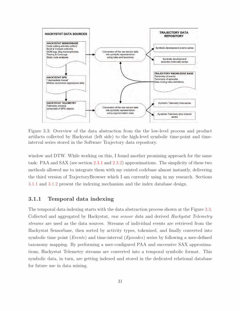
Figure 3.3: Overview of the data abstraction from the the low-level process and productartifacts collected by Hackystat (left side) to the high-level symbolic time-point and time-interval series stored in the Software Trajectory data repository.
window and DTW. While working on this, I found another promising approach for the same
task: PAA and SAX (see section 2.3.1 and 2.3.2) approximations. The simplicity of these two
methods allowed me to integrate them with my existed codebase almost instantly, delivering
the third version of TrajectoryBrowser which I am currently using in my research. Sections
3.1.1 and 3.1.2 present the indexing mechanism and the index database design.
3.1.1 Temporal data indexing
The temporal data indexing starts with the data abstraction process shown at the Figure 3.3.
Collected and aggregated by Hackystat, raw sensor data and derived Hackystat Telemetry
streams are used as the data sources. Streams of individual events are retrieved from the
Hackystat Sensorbase, then sorted by activity types, tokenized, and finally converted into
symbolic time point (Events) and time-interval (Episodes) series by following a user-defined
taxonomy mapping. By performing a user-configured PAA and successive SAX approxima-
tions, Hackystat Telemetry streams are converted into a temporal symbolic format. This
symbolic data, in turn, are getting indexed and stored in the dedicated relational database
for future use in data mining.
31

Figure 3.4: Overview of the current implementation of Software Trajectory framework.
I have not experimented with symbolic abstraction and mining of the raw sensor data
yet, but this approach has a solid foundation provided by Hongbing Kou, in his thesis
[34]. In his work, he was able to infer TDD behaviors by using a technique called Software
Development Stream Analysis (SDSA) which is very similar to mine, except the fundamental
difference in the approach: Hongbing defined TDD patterns at first and then search for them
using SDSA. Within SDSA, low-level software process data was first converted into symbolic
Episodes first. Next, sequences of Episodes (candidate patterns) were matched (aligned) to
the set of the known TDD temporal rules (patterns), and if they were found to satisfy TDD
rules (having sufficient support), the generative process was inferred as TDD.
I have implemented the indexing of Telemetry streams with a sliding window, PAA, and
SAX. I am using a sliding window approach following [37] for generating a set of subsequences
from a real-valued stream. Each of the subsequences is then normalized and converted into a
symbolic representation with PAA and SAX. This symbolic representation and the position
information is then stored in the relational database. For index manipulation and data
retrieval, I am using SQL. Figure 3.4 presents the current software system overview.
3.1.2 Index database design
Figure 3.5 presents the TrajectoryDB database schema in detail. This schema was designed
with two main requirements in mind. First, it must be able to hold a local copy of Teleme-
try streams due to the high time cost of querying Telemetry service remotely. Second, it
must support KDD algorithms through optimized SQL queries. Both goals were achieved,
resulting in high turn-around speed for both indexing and querying.
32

Figure 3.5: The database schema used for the Hackystat Telemetry data retrieval and in-dexing in the pilot project.
33
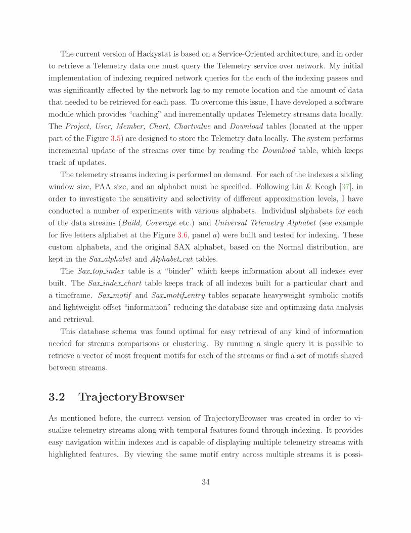
The current version of Hackystat is based on a Service-Oriented architecture, and in order
to retrieve a Telemetry data one must query the Telemetry service over network. My initial
implementation of indexing required network queries for the each of the indexing passes and
was significantly affected by the network lag to my remote location and the amount of data
that needed to be retrieved for each pass. To overcome this issue, I have developed a software
module which provides “caching” and incrementally updates Telemetry streams data locally.
The Project, User, Member, Chart, Chartvalue and Download tables (located at the upper
part of the Figure 3.5) are designed to store the Telemetry data locally. The system performs
incremental update of the streams over time by reading the Download table, which keeps
track of updates.
The telemetry streams indexing is performed on demand. For each of the indexes a sliding
window size, PAA size, and an alphabet must be specified. Following Lin & Keogh [37], in
order to investigate the sensitivity and selectivity of different approximation levels, I have
conducted a number of experiments with various alphabets. Individual alphabets for each
of the data streams (Build, Coverage etc.) and Universal Telemetry Alphabet (see example
for five letters alphabet at the Figure 3.6, panel a) were built and tested for indexing. These
custom alphabets, and the original SAX alphabet, based on the Normal distribution, are
kept in the Sax alphabet and Alphabet cut tables.
The Sax top index table is a “binder” which keeps information about all indexes ever
built. The Sax index chart table keeps track of all indexes built for a particular chart and
a timeframe. Sax motif and Sax motif entry tables separate heavyweight symbolic motifs
and lightweight offset “information” reducing the database size and optimizing data analysis
and retrieval.
This database schema was found optimal for easy retrieval of any kind of information
needed for streams comparisons or clustering. By running a single query it is possible to
retrieve a vector of most frequent motifs for each of the streams or find a set of motifs shared
between streams.
3.2 TrajectoryBrowser
As mentioned before, the current version of TrajectoryBrowser was created in order to vi-
sualize telemetry streams along with temporal features found through indexing. It provides
easy navigation within indexes and is capable of displaying multiple telemetry streams with
highlighted features. By viewing the same motif entry across multiple streams it is possi-
34

ble to guess information about coincidence of entries, as an example, see Section 4.4, for
sequential “growth” pattern finding experiment.
3.3 Future development roadmap
As I pointed out before, the current version of the TrajectoryBrowser and analyses do not
support processing of low-level raw Hackystat data and analyses based upon them. I have
already started the development of such a module along with extending the database schema
for storing raw data, its approximation, and taxonomy. Once these components are in place,
I will start developing data mining algorithms for Events and Episodes using the discussed
temporal data mining algorithms. Once all major software pieces are in place, I will focus
on the experimental evaluation of the system and improving the usability of the GUI.
35

Figure 3.6: The distribution of the Hackystat Telemetry data for a sample project dataset.While individual telemetry streams (panel b, left three plots for each stream represent rawdata, right three plots - Z-normalized data) show different data distributions, the combinedand normalized data (panel a) close to the normal distribution. Combined data was usedfor creation of the Universal Telemetry SAX alphabet.
36

Chapter 4
Experimental evaluation
I propose to conduct two case studies: Public data case study (Section 4.5), and Classroom
case study (Section 4.6) in order to empirically evaluate the capabilities and performance of
Software Trajectory framework. These studies differ in the granularity of data used, and in
the approaches for evaluation.
During my work on the pilot version of Software Trajectory framework, I began a set of
small experiments in order to aid in the architectural design and algorithms implementation.
In addition, these experiments helped me to outline the boundaries of applicability of my
approach to certain problems in software engineering. I call these experiments the Pilot
study and Section 4.4 discusses some of the insights yielded by this study.
My intent behind these empirical studies is to assess the ability of Software Trajectory
framework to recognize well known recurrent behavioral patterns and software processes (for
example Test Driven Development), as well as its ability to discover new ones. In addition,
these studies will support a classification and extension of the current Hackystat sensor
family in order to improve Software Trajectory’s performance. It is quite possible that some
of the currently collected sensor data will be excluded from the Software Trajectory datasets,
while some new ones will be designed and developed in order to capture important features
from the studied software development data streams.
Before proceeding with the presentation of design of these studies and approaches for
evaluation, I will discuss my evaluation paradigm.
37

4.1 Review of evaluation strategies
In contemporary literature, research methods are categorized into three paradigms: quan-
titative, qualitative and mixed-methods [46]. Despite the arguments presented in the past
for integrating first two methods [19], combining qualitative and quantitative methods in
a single, mixed-method study is currently widely practiced and accepted in many areas of
research, and in particular, in empirical software engineering [8] [48].
4.1.1 The two paradigms
The quantitative paradigm is based on positivism. The positivism philosophy presumes that
there exists only one truth, which is an objective reality independent from human perception,
which, in turn, means that a researcher and a researched phenomena is unable to influence
this truth or be influenced by it [19]. Quantitative studies are focused on finding of this
truth through extensive study of the phenomena, and often characterized with very large
sample sizes, control groups etc. in order to ensure proper statistical analysis.
In contrast, qualitative study is based on constructivism [15] [19] and interpretivism [1].
Both presume the existence of multiple truths based on the one’s construction of reality,
as well as non-existence of such a reality prior to the investigation. Moreover, once such a
reality is solely or socially constructed, it is not fixed, - it is changing over time, shaped by
new findings and experiences of researcher. Techniques of qualitative studies are not meant
to be applied to a large population. They rather focus on small, rich in features samples
which can provide valuable information. In other words, subjects in a qualitative study are
picked not because they represent large groups, but because they can articulate important
high-quality information.
The assumptions behind the two approaches extend beyond just methodological or philo-
sophical differences to the one’s perceptions of reality. According to Guba et al. [19], quali-
tative and quantitative methods do not study the same phenomena. Applying the authors’
statement to empirical software engineering, we can infer the limitations of qualitative stud-
ies by their inability to access some of the phenomena that researchers are interested in,
such as prior experiences, social interactions, and the behavioral variations of individuals
performing software process.
38
4.1.2 Mixed methods and Exploratory research
Surprisingly, the fundamental differences between the two paradigms are rarely discussed in
the mixed-methods research which is based on pragmatism. The finding of truth is more
important in pragmatist paradigm than the question of methods or philosophy. Researchers
practicing the mixed-method approach are free to use methods, techniques and protocols
which meet their purposes, and which, in the end, provide the best understanding of the
research problem. This unifying logic in understanding of studied phenomena regardless of
approach, is central to mixed methods.
While the three discussed paradigms at least assume the existence of a problem and
provide the outlines for methods of data collection and design of a study, sometimes a clear
statement of a problem is missing from research. In such a case, exploratory research must
be conducted in order to clarify the detailed nature of the problem.
4.2 Software Trajectory approach evolution
When I started exploring Hackystat telemetry streams during the Software Engineering
class taught by my present adviser Philip Johnson, I realized the “coolness” of software
process metrics visualization for providing insights into software process. By using the web
interface of Hackystat, I was able to pull and visualize various telemetry streams reflecting
my development. Working in the class, I compared metrics of my software process to ones
from my team members. Performing such analyses, and discussing their results enabled us
to improve our individual and team software processes, which resulted in excellent grades.
After joining CSDL, I started my research by exploring the boundaries of telemetry visu-
alization and telemetry analyses, and finding possibilities for improvements. At that point
of time, I was working on two problems: improving the visualization of telemetry streams
and introduction of metrics for quantitative comparison of telemetry streams (trajectories).
While working on these two problems, I realized that the real problem I am trying to solve lies
beyond the reach of these two. The problem is that the user is not provided with enough de-
tails about their software process to be able to perform comparative analyses of two projects
(two software processes). I am envisioning the solution of this problem through the extension
of Hackystat analyses with the ability to discover detailed features from software process.
In other words, by conducting exploratory research of visualization tools and techniques
as well as designing “flexible enough” metrics appropriate for telemetry streams comparison,
I have realized the importance of understanding of the generative software process. This
39

knowledge about performed software process, inferred from the set of collected artifacts, is
crucial in the process improvement and in the comparative analysis of software projects.
Once I was able to clearly formulate this problem, I have started another exploratory
study - my pilot study. By performing this exploration of the tools and techniques for
software process mining and inference, I am trying to build my own toolkit which will allow
me to approach the next problem - the problem of quantifying of software process through
the discovery of recurrent behaviors.
4.3 Software Trajectory case studies and evaluation
design
The proposed public data case study is based on the use of publicly available Software
Configuration Management (SCM) audit trails of the big, ongoing software projects such as
Eclipse, GNOME etc. Mining of SCM repositories is a well-developed area of research with
much work published [18]. SCM repositories contain coarse software product artifacts which
are usually mined with a purpose of discovering of various characteristics of software evolution
and software process. I am using a mixed-method approach in this study. In the first phase
of this study, I plan to perform SCM audit trail data mining following published work
and using Software Trajectory as a tool in order to discover confirmed patterns in software
process artifacts, and thus quantitatively evaluate Software Trajectory’s performance when
compared to existing tools. In the second phase, I will develop my own pre-processing and
taxonomy mapping of software process artifacts into temporal symbolic series. By using this
data and Software Trajectory framework, I plan to develop a new approach for SCM audit
trail mining and possibly discover new evolutionary behaviors within software process. These
discovered knowledge will be evaluated through the peer-reviewed publication submitted for
the annual MSR challenge [18].
The classroom case study is based on a more comprehensive data set. This data will
be collected by Hackystat from Continuous Integration and from individual developers and
will contain fine-grained information about performed software process. The approach I am
taking in this study is very similar to the public data case study. I will develop my own
taxonomy for mapping of software process artifacts into symbolic temporal data and will
apply Software Trajectory analyses to this data in order to discover recurrent behaviors. In
turn, these discovered knowledge will be evaluated through interviewing for usefulness and
meaningfulness. Results of interviewing will be used to improve Software Trajectory and
40
will constitute part of my thesis and following publication.
Both case studies are exploratory in nature. At this point of my research, I can only
see that the properties of my approach and its current implementation in the Software Tra-
jectory framework appear to be very promising. The wealth of developed techniques for
temporal symbolic data mining and recent development of SAX approximation allow me
to overcome many computational limitations in existing approaches for mining of software
process artifacts. The current implementation of Hackystat provides the ability to capture
fine-grain software product and process metrics providing a richness of data, which, poten-
tially, might reveal new insights. Current research in software process discovery indicates
the overall feasibility of proposed goals in the discovery of unknown recurrent behaviors in
software process.
Nevertheless, there is no prior knowledge about application of these techniques to soft-
ware process mining. Moreover, at this stage of my research, it is impossible to foresee
if new recurrent behaviors will be discovered or their meaningfulness or usefulness for real
world applications. For this reason I am undertaking a constructivism paradigm in my re-
search [15], and will develop knowledge about the applicability of my approach to software
process mining during the development of Software Trajectory framework and its empirical
evaluation. By designing, developing, deploying and observing a software system, and by
conducting interviews and surveys, I will gain the desired experience and knowledge.
But it is possible that this part of my research will fail, and I will not be able to discover
any meaningful novel knowledge about software process. If so, I will apply every effort to
investigate and explain the pitfalls of my approach to the domain of software process data
mining. It may be that failure is due to the specificity of domain, or due to the insufficiency of
the information enclosed in the collected artifacts, or maybe due to inefficiency of augmented
methods. Through thorough analyses of failed experiments and collection of feedback, I will
outline boundaries of the approach taken in this work and appropriate avenues for future
development.
4.4 Pilot study
In order to demonstrate the ability of Software Trajectory to perform telemetry indexing
and temporal recurrent patterns extraction, I have conducted two experiments which provide
insights in the use of the motif frequencies and software process event taxonomies.
41
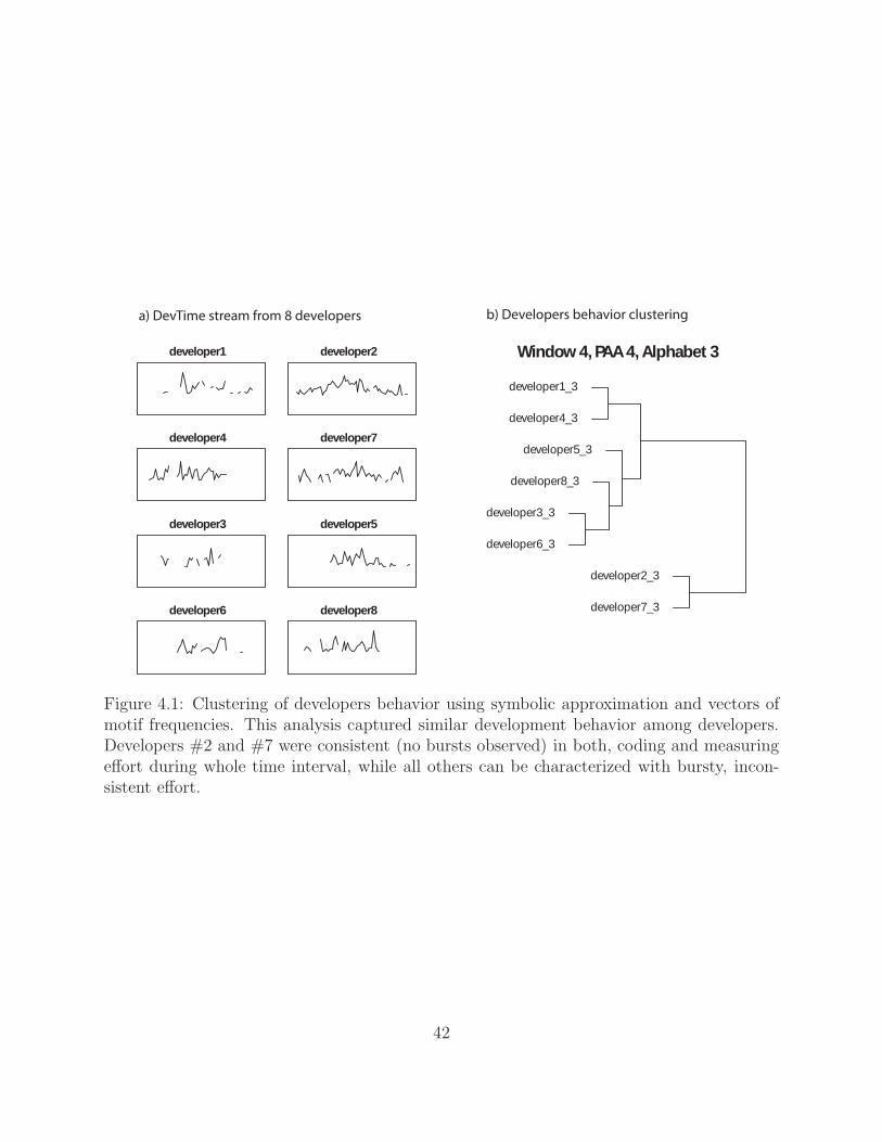
developer1_3
developer4_3
developer5_3
developer8_3
developer3_3
developer6_3
developer2_3
developer7_3
Window 4, PAA 4, Alphabet 3
a) DevTime stream from 8 developers b) Developers behavior clustering
developer1 developer2
developer4 developer7
developer3 developer5
developer6 developer8
Figure 4.1: Clustering of developers behavior using symbolic approximation and vectors ofmotif frequencies. This analysis captured similar development behavior among developers.Developers #2 and #7 were consistent (no bursts observed) in both, coding and measuringeffort during whole time interval, while all others can be characterized with bursty, incon-sistent effort.
42
4.4.1 Clustering of the Hackystat Telemetry streams
The main purpose of the this study was to evaluate the ability of PAA and SAX approx-
imations and indexing to capture a temporal specificity of telemetry streams through the
discovery of recurrent temporal patterns. Knowing about the frequently misleading results of
a time-series clustering [31], I did not expect to capture many interesting facts, nevertheless
the results were encouraging.
The data used in this study was collected from student users of Hackystat during Spring,
2009. This dataset represents Hackystat metrics collected during sixty days of a classroom
project by eight students. The following clustering experiments were conducted using the
distance between vectors of motif frequencies extracted by indexing of telemetry streams:
• Clustering of software process related telemetry streams collected from individual devel-
opers. I was able to group developers with similar behavioral patterns within clusters,
which indicates the feasibility of the classification approach. Figure 4.1 depicts results
of this analysis.
• Clustering of software product-related telemetry streams by using motif frequencies. I
was able to group telemetry streams, but while these groups look intuitively meaningful,
the close examination of the stream features suggests that this grouping happened due
to the similar temporal behavior on the short stretches. This result, while proving the
correctness of approach, indicates it’s limitation, pointing that instead of using just
motif frequencies, some temporal ordering should be taken into account. Figure 4.2
displays results of this analysis.
4.4.2 Sequential patterns search
The second pilot study, focusing on discovery of sequential patterns, was conducted using
real data from my own concurrent development of two software projects. While working on
the Software Trajectory framework, I made the decision to split the code into two parts:
an algorithm implementation library that I named JMotif, and user-interface part called
TrajectoryBrowser. While this decision simplified development, it introduced a dependency
of TrajectoryBrowser on the JMotif API. As a result of iterative and incremental pattern in
my development, I changed the JMotif public API three times, which consequently involved
extensive refactoring in the ProjectBrowser code. This dependency can be clearly seen from
observing DevTime streams at Figure 4.3 panel a.
43

CodeIssue_3
UnitTest_Failure_3
FileMetric_TotalLines_3
Churn_3
Coverage_NumCovered_3
Coverage_Percentage_3
CyclomaticComplexity
Coverage_NumUncovered_3
Build_failure_3
Commit_3
UnitTest_Success_3
UnitTest_Total_3
DevTime_3
Build_3
Build_success_3
Window 4, PAA 4, Alphabet 3
UnitTest_Total_5
UnitTest_Success_5
DevTime_5
FileMetric_5
Commit__5
Build_success_5
Build_success_5
Build_5
Build_failure_5
Coverage_NumUncovered_5
Churn__5
CyclomaticComplexity_5
Coverage_NumCovered_5
Coverage_Percentage_5
CodeIssue_5
UnitTest_Failure_5
Window 5, PAA 5, Alphabet 5
CodeIssue Build
UnitTest_Failure Build_success
UnitTest_SuccessCount DevTime
UnitTest_TotalCount Build_failure
CyclomaticComplexity Commit
Coverage_NumUncovered Coverage_NumCovered
Churn Coverage_Percentage
FileMetric_TotalLines
a) Telemetry streams for Pilot dataset b) Telemetry strems clustering with different settings
Figure 4.2: Clustering of telemetry streams for classroom pilot dataset using symbolic ap-proximation and vectors of motif frequencies. While it seems to be meaningful to findcorrelation between UnitTest Failure and CodeIssue streams unit test, this grouping hap-pened due to the similarity of behavior pattern - short, high amplitude bursts; but note,there is no correlation of features in time .
44

Figure 4.3: The illustration of finding of sequential growth pattern in two DevTime telemetrystreams. Panel a: The Hackystat ProjectBrowser showing telemetry streams. Panel b: theTrajectoryBrowser showing same telemetry streams along with identified pattern. Panel c:the symbolic representation of streams with highlighted pattern.
In order to capture this dependency pattern in two Telemetry streams, representing the
daily amount of development time spent on the TrajectoryBrowser and JMotif projects, I
defined a synthetic growth pattern as the large positive delta value between previous and
current day effort. By transforming Telemetry streams with this simple rule in the symbolic
form, I obtained a two dimensional symbolic time series, where letter G represents a growth
pattern, see Figure 4.3 panel c. I defined a formal rule for sequential growth pattern as the
pattern like GJMotif → GTrajectoryBrowser where distance between these Gs is less than three
days. By application of this rule I identified a pattern which exactly corresponds to my
experience.
While this experiment was designed with a purpose and does not provide any value in
the dependencies discovery, the “sequential growth” pattern and past effort information can
be used in the estimation of effort needed for requested software changes.
4.5 Public data case study
I plan to evaluate my research and its results through the mining of publicly available
software configuration management (SCM) repositories. The goal of this experiment is to
45
assess the ability of my approach to reproduce already published results, which will indicate
the correctness of approach taken, along with the ability to compare the performance of
Software Trajectory to other tools. If I can find novel patterns within this data with my
approach, it will provide additional evidence for the utility of my research.
As the main source of the data, I am planning to use public SCM repositories whose
mining is traditionally used in the “MSR Challenges” [18] and published in proceedings of
“IEEE International Conference on Mining Software Repositories”. The GNOME project
SCM data will be used in the 2009 challenge, Eclipse repositories were used in 2008 and 2007;
PostgreSQL and ArgoUML in 2006. Two primary temporal data sets are usually offered for
use: one is the CVS repository audit trail and second one is the bugs and issues tracking
information. The following MSR challenge topics I found relevant to my research:
• Approaches, applications, and tools for software repository mining.
• Analysis of change patterns to assist in future development.
• Prediction, characterization, and classification of software defects based on analysis of
software repositories.
• Techniques to model reliability and defect occurrences.
My approach will be based on the approximation of the artifacts from SCM repositories into
symbolic series using “SCM trail taxonomy” and successful indexing of this symbolic data.
For example, in order to find “ripple effect” patterns in software change, I will construct
a set of symbolic time-points and time-interval series which will represent all code changes
in time by pre-processing change metadata from issue tracking system and actual changes
in version control by using sliding window. Once data will be extracted and saved locally,
for time-points symbolic data I will construct a series for each of the software packages (like
eclipse.swt.layout.*, org.eclipse.swt.widgets.*, etc.) where symbolic data repre-
sents a change occurred in the package. For time-interval symbolic data I will use the dura-
tion when a change request was “open” to construct series representing concurrent order and
dynamics of changes. By applying Software Trajectory analyses, I expect to discover some-
thing like “the change requested in package A class b usually results in changes in package
A class c and package B class d” and it takes Abt + Act + Bdt time to finish these changes.
In turn, this information can be used to estimate the time and effort of newly requested
software changes as well, as to identify changes that more likely to induce bugs and fixes
and should be avoided. By adding the information about developers working on fixes, it is
46

also possible to design an expert system which will suggest assignment of newly reported
bug reports or feature request to a particular developer(s).
In addition to the public SCM, there are various public data hosted by the “PROMISE
software engineering repository” [47] which contains two kinds of data: the software product
datasets used for the building of the predictive software models, and some “universal” data
sets representing SCM repository transaction. Most of these datasets were also used for
a number of publications and I am planning to evaluate my framework by attempting to
reproduce these results.
4.6 Classroom study
In order to evaluate Software Trajectory performance in the discovery of well known and novel
recurrent behavioral patterns in software process, I am planning to conduct two classroom
case studies followed by survey of participants (Section 6.1).
The studies will be conducted in two Software Engineering classes during the Fall’09
semester (ICS 413 and ICS 613) and one software engineering class (ICS 414) during the
Spring’10 semesters taught by Dr. Philip Johnson at the University of Hawaii. ICS 413 and
ICS 414 are for undergraduate students, and ICS 613 is for graduate students. By curriculum
design, students will be required to collect metrics and perform analyses on their own data in
order to develop understanding of software metrics and improve their software development
process. About 20 - 30 students are expected to participate in the study.
By the beginning of the data collection in the Fall’09 class I am planning to implement
a data extraction, transformation and indexing engine, and begin the first phase of the
classroom study. This engine will perform unsupervised recurrent behaviors discovery on the
daily basis. By the end of the class I will administer interviews to collect students feedback
about Software Trajectory analyses. The questionnaire will cover questions concerned about
Software Trajectory analyses performance and usability. Another important question will
be the students’ perception of whether or not Software Trajectory analyses is a reasonable
approach to software process discovery, analysis and improvement in “real world” settings.
The experience collected during the first phase of the classroom study will be used in the
improvement of the Software Trajectory analyses and in the design of the TrajectoryBrowser
user interface.
By the beginning of the data collection in the Spring’10 class I am planning to release a
next version of the Software Trajectory analyses framework incorporating experience from
47

the first classroom study. The second classroom study will be very similar to the first one
in the flow.
4.6.1 Classroom study design
As explained before, during the classroom study the software product and process data will
be collected from continuous integration as well as from individual students by Hackystat.
This data will be converted into a symbolic representation and analyzed with Software
Trajectory. Once Software Trajectory identifies strongly supported (“candidate”) patterns,
they will be analyzed by me.
The support function I am considering for this study will be a product of two metrics:
the first one is based on the support function from the AprioriAll algorithm and will quantify
the fraction of participating students demonstrating the pattern, and the second one is based
on the total frequency of the pattern appearance. The reason for using two components is
that the classroom “sampling space” is limited to only twenty students and it is likely that
there will be “non-shared” strong patterns - ones that observed only within a data collected
from the single student.
I understand that this choice of the support function introduces a bias into my analyses
by focusing too much on subjective patterns which might be too specific to the observed
individuals or classroom curriculum settings. Here I am compromising between the ability
to capture recurrent behaviors at all and the usefulness and significance of captured behav-
iors. As I said, at this point of my research it is impossible to foresee the cognitive impact
of observing and understanding of discovered patterns and guess where I should draw the
support function threshold. By iteratively reviewing Software Trajectory results and collect-
ing relevant feedback from students through the instructor, I plan to improve the Software
Trajectory knowledge base in order to prune reported patterns to only useful and meaningful
ones. This ability to communicate with students and iteratively improve the system design
is crucial for in-process knowledge development and overall experiment success.
I am planning to perform two types of analyses: an individual developer behavioral
software process analysis (personal software process discovery) and a “collective software
process” analysis.
48

Symbolic abbreviation Descriptionof Events
CI code implementation event,corresponds to the new code entry
CR code refactoring event, includes renamingor deleting of functional units, and buffer transactions
CD debugging eventCCS successful compilation eventCCF unsuccessful compilation eventUTS successful unit test runUTF unsuccessful unit test runCM code commit to version controlCU code update from version controlCAS code analysis success event, corresponds to a
successful invocation of one of the code analysis toolsCAF code analysis failure event, corresponds to a
unsuccessful invocation of one of the code analysis toolsCCP positive delta in the code size (churn)CCN negative delta in the code size (churn)
Table 4.1: Taxonomy of the Symbolic Events to be used in the classroom evaluation ofSoftware Trajectory analyses.
49

4.6.2 Personal software process discovery
For this type of experimental validation, I plan to perform Software Trajectory analyses
using Hackystat data collected from individual developers. The data collected by Hackystat
from each of developers will be aggregated into symbolic streams of two types: symbolic
Events series and symbolic Episodes series:
• Symbolic Events series. This dataset will consist of the thirteen types of Events listed
in Table 4.1. These Events represent a set of essential code-development activities
which will constitute a multivariate symbolic time-point series for further analyses
through data mining. The goal of these analyses will be to discover recurrent behavioral
patterns in the sequence of activities by an individual developer.
• Symbolic Episodes data. This dataset will consist of the fifteen types of Episodes listed
in the table 4.2. These Episodes represent a set of code-development activities which
intended to capture dynamic recurrent behavioral patterns.
The goal of the Event series analysis is to build a taxonomy of symbolic software pro-
cess patterns corresponding to one of the behaviors such as test-driven design or the more
traditional test-last design.
In contrast to the analysis of symbolic Events series, which treats the process as a set of
sequential activities, the analysis of symbolic Episodes series is intended to support discovery
of overlapping, dynamic patterns. For example, I might find that an unsuccessful unit testing
episode is usually happening within a code refactoring episode.
By combining Events and Episodes in the analyses I might discover that during code
implementation, unit tests are usually successful but accompanied with decreasing test cov-
erage. Also, I expect to be able to infer a developers’ “reaction” patterns. For example, as
a reaction to the continuous failure of unit tests, one might start broad refactoring of the
code with the goal of reducing its complexity.
4.6.3 Team-based software process discovery
Traditionally students in the class work in groups. It will be interesting to see whether the
“team-based behavior” and corresponding recurrent behavioral patterns are different from
those in the personal software process. For the “team-based software process” recurrent
behavioral pattern discovery I plan to summarize individual developer streams by combining
overlapping Events and Episodes of same activities. It is hard to guess at this time whether
50

Symbolic abbreviation Descriptionof Episodes of metric
CI code implementation episode,corresponds to new code entry events
CR code refactoring episode, includes renamingor deleting of functional units, and buffer transactions
CD code debugging episode,corresponds to debugging events
CCS successful code compilation episode, correspondsto two or more successful compilation events
CCF unsuccessful code compilation episode, correspondsto two or more unsuccessful compilation events
UTS successful unit test episode, correspondsto two or more successful unit-test events
UTF unsuccessful unit test episode, correspondsto two or more unsuccessful unit-test events
TCG code test coverage growth, corresponds to a positivedelta between at least three code coverage analysistool invocations
TCD code test coverage decrease, corresponds to a negativedelta between at least three code coverage analysistool invocations
CSG code size growth, corresponds to a positivedelta between at least three code size analysistool invocations or three commits
CSD code size decrease, corresponds to a negativedelta between at least three code size analysistool invocations or three commits
CCG code complexity growth, corresponds to a positivedelta between at least three complexity analysistool invocations
CCD code complexity decrease, corresponds to a negativecode complexity delta between at least three complexityanalysis tool invocations
CAS “clean code development” episode, corresponds toat least three successful code analysis tools invocations
CAF “unclean code development” episode, corresponds toat least three unsuccessful code analysis tools invocations
Table 4.2: Taxonomy of the Symbolic Episodes to be used in the classroom evaluation ofSoftware Trajectory analyses.
51

or not these aggregated streams will be more or less noisy than individual streams, but in any
case the application of the Software Trajectory analyses might lead to interesting findings.
For example, I might infer a “programming session” episodes through the high fraction
of synchronous (overlapping) development events between team members, or identify role
separation by analyzing each student’s development/commit patterns.
52

Chapter 5
Summary and Future Directions
5.1 Contribution
The main contribution of my research to the software engineering and software process com-
munity is the development and evaluation of a previously unexplored approach to discovering
of recurrent behaviors in software process through the temporal data mining of low-level pro-
cess and product artifacts.
The knowledge developed through the experimental work, and evaluation of the approach
taken, will be another contribution of my research. By performing these experiments, I also
hoping to discover new patterns in software process and software evolution thereby improving
our knowledge about it.
The software framework and data mining toolkit which I will develop for my research
will be integrated with the existing family of Hackystat tools and made available as open
source, thus contributing to the software-engineering community.
5.2 Estimated Timeline
By the beginning of the Fall’09 semester, I plan to design a taxonomy and implement a low-
level software process artifact abstractions into a symbolic representation for the classroom
experiments. The current database schema will be extended for storing these data and
indexes. Immediately after that, I will proceed with the implementation of fundamental
algorithms for sequential patterns mining from the time-points and time-interval data. My
goal is to have a first-generation data model and KDD toolkit to be available for use before
in-class development starts.
53

Sep-09 Oct-09 Nov-09 Dec-09 Jan-10 Feb-10 Mar-10 Apr-10 May-10 Jun-10 Jul-10 Aug-10
Dec - Feb
Trajectory improvementsbased on the results ofclassroom experiment
Feb - May
MSR Callengemining experiments
and paper submission
FebTrajectory v.2.0
JunTrajectory v.3.0
May - Aug
Thesis & peer-reviewed publication writing
Aug - OctDevelopment of Events & Episodes
approximations, data mining algorithms & TrajectoryBrowser
OctTrajectory v.1.0
Oct - DecThe Fall’09 classroom experiment
SepThesis defense
Feb - MayThe Spring’10 classroom experiment
MayMSR Challenge,
paper submission deadline
JanMSR Challenge,abstract deadline
Figure 5.1: Proposed Software Trajectory development timeline.
Based on the Fall’09 classroom experiment experience, I will extend and fine-tune my
system for the Spring’10 software engineering class, during which I plan to evaluate a final
version of my system. The results of these two classroom experiments, the description of
designed methods and developed software will constitute a peer-reviewed publication which
I plan finish by Summer’10.
The MSR Challenge 2010 is announced to happen early May’10. I plan to design SCM
data mining toolkit and perform pilot experiments by early January’10 submitting an ab-
stract. If abstract will be accepted, I will prepare and submit a research paper following the
Challenge timeline.
I plan to be working on my thesis during Fall’09, Spring’10 and Summer’10 semesters.
During the Fall’10 semester I plan to finish my work and defend the dissertation.
54

Chapter 6
Appendices
6.1 Classroom case study interview design
I plan to conduct at least one classroom interview session evaluating Software Trajectory
framework. I am targeting senior-level undergraduates and graduate students as my primary
responders. These interviews will be conducted under approved by Committee on Human
Subjects application: CHS #16520 - Evaluation of Hackystat. By performing interviews,
I expect to collect evidence about the ability of Software Trajectory framework to capture
recurrent behaviors from software process performed on the team and individual level. My
secondary goal is the evaluation of the significance of these behaviors for software process
understanding and improvement.
I plan to administer interviews during the last week of instructions. I will select respon-
ders demonstrating recurrent behaviors by balancing two factors: first is to cover as much
various discovered patterns as possible, and second is to cover patterns demonstrated by the
most of students. Taking in account the possible students’ concern about final grading, I am
crafting my interview questionnaire in order to make it as neutral as possible. The current
version of the interview questionnaire is presented further.
The first three questions are designed to assess the respondents’ level of education, area
of expertise, and knowledge of software development patterns. The fourth question elicits
a general discussion to the classroom experience and the respondents’ opinion about the
software processes they performed and I observed. By introducing my research in greater
detail at this point, and by walking through the last three questions I will try to encourage
responder to discuss with me my findings. Depending on the responders’ reaction and
willingness to continue, I will finish the interview after two to five iterations over observed
55

patterns.
The interviews will be tape-recorded, later they will be transcribed, coded, and ana-
lyzed. I am not very familiar with a methodology of developing of coding procedures yet,
moreover, at this point of time it is impossible to foresee any of the results of Software Trajec-
tory analyses. Thus, interview coding scheme will be constructed after interview-discussed
(“candidate”) patterns will be identified.
6.1.1 Software Trajectory evaluation interview questionnaire
1. What is your level of education and major?
2. Do you have any previous experience with software development?
3. Do you aware about recurrent behaviors (philosophies/approaches/styles) in the soft-
ware development? If so, which ones can you recall?
4. Did you ever follow any of the formal approaches or styles in your own, professional,
or the classroom development?
5. By applying Software Trajectory framework I was able to capture a behavioral pattern
P which looks like P1 → P2 → .... My interpretation of this is .... . Does my interpre-
tation of this recurrent behavior match your own understanding of your development
behavior?
6. Is there another interpretation of this pattern that you believe more accurately reflects
your behavior?
7. When you think about this pattern, can you think of changes you might want to make
to your development behaviors based upon it?
56

6.1.2 Software Trajectory consent form
Thank you for agreeing to participate in our research on software process discovery. This
research experiment is being conducted by Pavel Senin as a part of his Ph.D. research in
Computer Science under the supervision of Professor Philip Johnson.
As a part of this research experiment, you will be asked to provide a feedback about
automatically discovered behavioral patterns in your software development process. These
patterns will be automatically discovered by Software Trajectory framework which applies
data mining techniques to the telemetry streams collected by Hackystat. The primary goal
of this research is to evaluate the ability of Software Trajectory to discover and classify re-
current behavioral patterns; while the secondary goal is to assess the usefulness of discovered
behaviors.
The data that we collect will be kept anonymously, and there will be no identifying
information about you in any analyses of this data.
Your participation is voluntary, and you may decide to stop participation at any time,
including after your data has been collected. If you are doing this task as part of a course,
your participation or lack of participation will not affect your grade.
If you have questions regarding this research, you may contact Professor Philip Johnson,
Department of Information and Computer Sciences, University of Hawaii, 1680 East-West
Road, Honolulu, HI 96822, 808-956-3489. If you have questions or concerns related to your
treatment as a research subject, you can contact the University of Hawaii Committee on
Human Studies, 2540 Maile Way, Spalding Hall 253, University of Hawaii, Honolulu, HI
96822, 808-539-3955.
Please sign below to indicate that you have read and agreed to these conditions.
Thank you very much!
Your name/signature
Cc: A copy of this consent form will be provided to you to keep.
57

Bibliography
[1] Handbook of Qualitative Research. Sage Publications, Inc, 2nd edition, March 2000.
[2] R. Agrawal and R. Srikant. Mining sequential patterns. pages 3–14, 1995.
[3] Rakesh Agrawal, Dimitrios Gunopulos, and Frank Leymann. Mining process models
from workflow logs. pages 467–483. 1998.
[4] James F. Allen. Maintaining knowledge about temporal intervals. Commun. ACM,
26(11):832–843, November 1983.
[5] Thomas A. Alspaugh. Allen’s interval algebra. webpage.
[6] Fabio L. Bellifemine, Giovanni Caire, and Dominic Greenwood. Developing Multi-Agent
Systems with JADE (Wiley Series in Agent Technology). Wiley, April 2007.
[7] A. W. Biermann and J. Feldman. On the synthesis of finite-state machines from samples
of their behavior. IEEE Trans. Computers, pages 592–597, 1972.
[8] Marcus Ciolkowski and Andreas Jedlitschka. Experience on applying quantitative and
qualitative empiricism to software engineering. pages 402–404. 2007.
[9] Paul Cohen. Fluent learning: Elucidating the structure of episodes. pages 268–277.
2001.
[10] Reidar Conradi. SPI frameworks: TQM, CMM, SPICE, ISO 9001, QIP experiences and
trends - norwegian SPIQ project.
[11] Jonathan E. Cook. Process discovery and validation through event-data analysis. PhD
thesis, Boulder, CO, USA, 1996.
[12] Jonathan E. Cook, Zhidian Du, Chongbing Liu, Alexander L. Wolf, and Er. Discovering
models of behavior for concurrent workflows, 2004.
58

[13] Jonathan E. Cook and Alexander L. Wolf. Discovering models of software processes
from event-based data. ACM Trans. Softw. Eng. Methodol., 7(3):215–249, July 1998.
[14] J. Cortadella, M. Kishinevsky, L. Lavagno, and A. Yakovlev. Deriving petri nets from
finite transition systems. Computers, IEEE Transactions on, 47(8):859–882, 1998.
[15] John W. Creswell. Research Design: Qualitative, Quantitative, and Mixed Methods
Approaches (2nd Edition). Sage Publications, Inc, 2nd edition, July 2002.
[16] Hui Ding, Goce Trajcevski, Peter Scheuermann, Xiaoyue Wang, and Eamonn Keogh.
Querying and mining of time series data: experimental comparison of representations
and distance measures. Proc. VLDB Endow., 1(2):1542–1552, 2008.
[17] Christian Freksa. Temporal reasoning based on semi-intervals. Artif. Intell., 54(1-
2):199–227, 1992.
[18] Harald Gall, Michele Lanza, and Thomas Zimmermann. 4th international workshop on
mining software repositories (MSR 2007). In Software Engineering - Companion, 2007.
ICSE 2007 Companion. 29th International Conference on, pages 107–108, 2007.
[19] Egon G. Guba and Yvonna S. Lincoln. Competing paradigms in qualitative research.
In Norman K. Denzin and Yvonna S. Lincoln, editors, The Landscape of Qualitative
Research, pages 195–220. Sage, 1998.
[20] G. Guimaraes. A method for automated temporal knowledge acquisition applied to
sleep-related breathing disorders. Artificial Intelligence in Medicine, 23(3):211–237,
November 2001.
[21] Jiawei Han and Micheline Kamber. Data Mining, Second Edition, Second Edition :
Concepts and Techniques (The Morgan Kaufmann Series in Data Management Systems)
(The Morgan Kaufmann Series in Data Management Systems). Morgan Kaufmann,
January 2006.
[22] Frank Hoppner. Discovery of temporal patterns - learning rules about the qualitative
behaviour of time series, 2001.
[23] Chris Jensen and Walt Scacchi. Guiding the discovery of open source software processes
with a reference model. pages 265–270. 2007.
59
[24] Linhui Jiang and Howard Hamilton. Methods for mining frequent sequential patterns.
page 992. 2003.
[25] Philip M. Johnson, Shaoxuan Zhang, and Pavel Senin. Experiences with hackystat as a
service-oriented architecture. Technical Report CSDL-09-07, Department of Information
and Computer Sciences, University of Hawaii, Honolulu, Hawaii 96822, Los Angeles,
California, February 2009.
[26] Neil C. Jones and Pavel A. Pevzner. An Introduction to Bioinformatics Algorithms
(Computational Molecular Biology). The MIT Press, August 2004.
[27] Huzefa Kagdi, Michael L. Collard, and Jonathan I. Maletic. A survey and taxonomy
of approaches for mining software repositories in the context of software evolution. J.
Softw. Maint. Evol., 19(2):77–131, 2007.
[28] Huzefa Kagdi, Shehnaaz Yusuf, and Jonathan I. Maletic. Mining sequences of changed-
files from version histories. In MSR ’06: Proceedings of the 2006 international workshop
on Mining software repositories, pages 47–53, New York, NY, USA, 2006. ACM.
[29] Po-Shan Kam and Ada W. Fu. Discovering temporal patterns for interval-based events.
In Proceedings of the 2nd International Conference on Data Warehousing and Knowl-
edge Discovery (DaWaK’00, pages 317–326, 2000.
[30] Eamonn Keogh, Kaushik Chakrabarti, Michael Pazzani, and Sharad Mehrotra. Dimen-
sionality reduction for fast similarity search in large time series databases. Knowledge
and Information Systems, 3(3):263–286, 2001.
[31] Eamonn Keogh, Jessica Lin, and Wagner Truppel. Clustering of time series subsequences
is meaningless: Implications for previous and future research. In ICDM ’03: Proceedings
of the Third IEEE International Conference on Data Mining, Washington, DC, USA,
2003. IEEE Computer Society.
[32] Eamonn Keogh, Stefano Lonardi, and Bill ’. Chiu. Finding surprising patterns in a
time series database in linear time and space. In KDD ’02: Proceedings of the eighth
ACM SIGKDD international conference on Knowledge discovery and data mining, pages
550–556, New York, NY, USA, 2002. ACM.
60

[33] Sunghun Kim, E. James Whitehead, and Jennifer Bevan. Properties of signature change
patterns. In ICSM ’06: Proceedings of the 22nd IEEE International Conference on Soft-
ware Maintenance, pages 4–13, Washington, DC, USA, 2006. IEEE Computer Society.
[34] Hongbing Kou. Automated Inference of Software Development Behaviors: Design, Im-
plementation and Validation of Zorro for Test-Driven Development. Ph.D. thesis, Uni-
versity of Hawaii, Department of Information and Computer Sciences, December 2007.
[35] Richard J. Larsen and Morris L. Marx. An Introduction to Mathematical Statistics and
Its Applications (3rd Edition). Prentice Hall, 3rd edition, January 2000.
[36] Jessica Lin, Eamonn Keogh, Stefano Lonardi, and Bill Chiu. A symbolic representation
of time series, with implications for streaming algorithms. In DMKD ’03: Proceedings
of the 8th ACM SIGMOD workshop on Research issues in data mining and knowledge
discovery, pages 2–11, New York, NY, USA, 2003. ACM Press.
[37] Jessica Lin, Eamonn Keogh, Li Wei, and Stefano Lonardi. Experiencing SAX: a
novel symbolic representation of time series. Data Mining and Knowledge Discovery,
15(2):107–144, October 2007.
[38] Benjamin Livshits and Thomas Zimmermann. Dynamine: Finding common error pat-
terns by mining software revision histories. In In ESEC/FSE, pages 296–305, 2005.
[39] David Lo, Hong Cheng, Jiawei Han, Siau C. Khoo, and Chengnian Sun. Classification
of software behaviors for failure detection: a discriminative pattern mining approach. In
KDD ’09: Proceedings of the 15th ACM SIGKDD international conference on Knowl-
edge discovery and data mining, pages 557–566, New York, NY, USA, 2009. ACM.
[40] Peiwei Mi and Walt Scacchi. A meta-model for formulating knowledge-based models of
software development, 1994.
[41] Fabian Morchen. Unsupervised pattern mining from symbolic temporal data. SIGKDD
Explor. Newsl., 9(1):41–55, June 2007.
[42] Fabian Morchen and Alfred Ultsch. Mining hierarchical temporal patterns in multi-
variate time series. In Susanne Biundo, Thom Fruhwirth, and Gunther Palm, editors,
KI 2004: Advances in Artificial Intelligence, volume 3238 of Lecture Notes in Artificial
Intelligence, pages 127–140. Springer, Berlin / Heidelberg, Germany, 2004.
61
[43] Luigi Palopoli and Giorgio Terracina. Discovering frequent structured patterns from
string databases: An application to biological sequences. pages 283–296. 2008.
[44] Chris P. Rainsford and John F. Roddick. Adding temporal semantics to association
rules. In PKDD ’99: Proceedings of the Third European Conference on Principles of
Data Mining and Knowledge Discovery, pages 504–509, London, UK, 1999. Springer-
Verlag.
[45] Vladimir Rubin, Christian Gunther, Wil van der Aalst, Ekkart Kindler, Boudewijn van
Dongen, and Wilhelm Schafer. Process mining framework for software processes. pages
169–181. 2007.
[46] Joanna E. M. Sale, Lynne H. Lohfeld, and Kevin Brazil. Revisiting the quantitative-
qualitative debate: Implications for mixed-methods research. Quality and Quantity,
36(1):43–53, February 2002.
[47] J. Sayyad Shirabad and T. J. Menzies. The PROMISE Repository of Software Engi-
neering Databases. School of Information Technology and Engineering, University of
Ottawa, Canada, 2005.
[48] Susan E. Sim, Janice Singer, and Margaret-Anne Storey. Beg, borrow, or steal: Us-
ing multidisciplinary approaches in empirical software engineering research. Empirical
Software Engineering, 6(1):85–93, March 2001.
[49] C. G. M. Snoek and M. Worring. Multimedia event-based video indexing using time
intervals. Multimedia, IEEE Transactions on, 7(4):638–647, 2005.
[50] Esko Ukkonen. On-line construction of suffix trees. Algorithmica, 14(3):249–260, 1995.
[51] Univ, Harald Gall, and Karin Hajek. Detection of logical coupling based on product
release history, 1998.
[52] W. van der Aalst, V. Rubin, H. Verbeek, B. van Dongen, E. Kindler, and C. Gunther.
Process mining: a two-step approach to balance between underfitting and overfitting.
Software and Systems Modeling, 2009.
[53] W. M. P. van der Aalst, Alves K. A. de Medeiros, and A. J. M. M. Weijters. Genetic
process mining. pages 48–69. 2005.
62
[54] B. F. van Dongen, A. K. A. de Medeiros, H. M. W. Verbeek, A. J. M. M. Weijters,
and W. M. P. van der Aalst. The ProM framework: A new era in process mining tool
support. pages 444–454. 2005.
[55] M. Vilain. A system for reasoning about time. In 2nd National (US) Conference on
Artificial Intelligence, pages 197–201. AAAI Press, 1982.
[56] Roy Villafane, Kien A. Hua, Duc Tran, and Basab Maulik. Mining interval time series.
In Data Warehousing and Knowledge Discovery, pages 318–330, 1999.
[57] J. Vilo. Discovering frequent patterns from strings. Technical report, University of
Helsinki, Finland, 1998.
[58] Ching Y. Wang, Tzung P. Hong, and Shian S. Tseng. Maintenance of sequential patterns
for record deletion. Data Mining, IEEE International Conference on, 0:536+, 2001.
[59] A. J. M. M. Weijters and W. M. P. van der Aalst. Rediscovering workflow models from
event-based data using little thumb. Integr. Comput.-Aided Eng., 10(2):151–162, 2003.
[60] Dragomir Yankov, Eamonn Keogh, Jose Medina, Bill Chiu, and Victor Zordan. De-
tecting time series motifs under uniform scaling. In KDD ’07: Proceedings of the 13th
ACM SIGKDD international conference on Knowledge discovery and data mining, pages
844–853, New York, NY, USA, 2007. ACM.
[61] Byoung-Kee Yi and Christos Faloutsos. Fast time sequence indexing for arbitrary Lp
norms. In VLDB ’00: Proceedings of the 26th International Conference on Very Large
Data Bases, pages 385–394, San Francisco, CA, USA, 2000. Morgan Kaufmann Pub-
lishers Inc.
[62] A. T. T. Ying, G. C. Murphy, R. Ng, and M. C. Chu-Carroll. Predicting source
code changes by mining change history. Software Engineering, IEEE Transactions on,
30(9):574–586, September 2004.
[63] Mohammed J. Zaki and Ching J. Hsiao. Efficient algorithms for mining closed itemsets
and their lattice structure. IEEE Transactions on Knowledge and Data Engineering,
17(4):462–478, 2005.
[64] Thomas Zimmermann, Sunghun Kim, Andreas Zeller, and E. James Whitehead. Mining
version archives for co-changed lines. In MSR ’06: Proceedings of the 2006 international
63

workshop on Mining software repositories, pages 72–75, New York, NY, USA, 2006.
ACM.
64