software tools for the supervisory control of petri nets based on place invariants

Software Tools for the Supervisory Control of Petri Nets Basedon Place Invariants

Technical Report of the ISIS Group

at the University of Notre Dame

ISIS-2002-003

April, 2002

Marian V. Iordache and Panos J. Antsaklis

Department of Electrical Engineering

University of Notre Dame

Notre Dame, IN 46556, USA

E-mail: [email protected], [email protected]

Interdisciplinary Studies of Intelligent Systems

M.V. Iordache, P.J. Antsaklis, “Software Tools for the Supervisory Control of Petri Nets Based on Place Invariants,” ISIS Technical Report ISIS-2002-003, April 2002.

Software Tools for the Supervisory Control of Petri Nets Based on

Place Invariants∗

Marian V. Iordache and Panos J. Antsaklis

Department of Electrical Engineering,

University of Notre Dame, IN 46556

E-mail: iordache.1, [email protected]

This document describes a Matlab toolbox for the supervisory control of Petri nets based on place

invariants [8, 10]. In what follows we present a detailed description of a number of functions we

propose. These are the topics we address:

• Solving integer programs

• Transformations to admissible marking constraints

• Enforcing linear constraints in Petri nets which may have uncontrollable and/or unobservabletransitions

• Invariant computation

• The coverability (reachability) graph

• Deadlock prevention and liveness enforcement

This document does not present all functions of the toolbox, as some of the functions are typically

used only as subroutines of the main functions. However, all functions are provided with detailed

help lines which can be read using the help command of Matlab.

The software was developed under Matlab 5.3 and Matlab 6 on a SunOS platform.

∗The partial support of the Lockheed Martin Corporation, the Army Research Office (DAAG55-98-1-0199), the

National Science Foundation (NSF ECS99-12458), and the DARPA/ITO-NEST Program (AF-F30602-01-2-0526) is

gratefully acknowledged.


2

Contents

Integer Programming 3

IP SOLVE . . . . . . . . . . . . . . . . . . . . . . . . . . . . . . . . . . . . . . . . . . . . . 3

Petri Nets 5

GETPN . . . . . . . . . . . . . . . . . . . . . . . . . . . . . . . . . . . . . . . . . . . . . . 5

The Coverability Graph 6

PNCGRAPH . . . . . . . . . . . . . . . . . . . . . . . . . . . . . . . . . . . . . . . . . . . 6

Enforcing Linear Constraints 8

MRO ADM . . . . . . . . . . . . . . . . . . . . . . . . . . . . . . . . . . . . . . . . . . . . 8

ILP ADM . . . . . . . . . . . . . . . . . . . . . . . . . . . . . . . . . . . . . . . . . . . . . 10

LINENF . . . . . . . . . . . . . . . . . . . . . . . . . . . . . . . . . . . . . . . . . . . . . . 11

ISADM . . . . . . . . . . . . . . . . . . . . . . . . . . . . . . . . . . . . . . . . . . . . . . 14

Invariant Computation 16

NULL . . . . . . . . . . . . . . . . . . . . . . . . . . . . . . . . . . . . . . . . . . . . . . . 16

INVAR . . . . . . . . . . . . . . . . . . . . . . . . . . . . . . . . . . . . . . . . . . . . . . 17

Deadlock Prevention 19

DP . . . . . . . . . . . . . . . . . . . . . . . . . . . . . . . . . . . . . . . . . . . . . . . . . 19

Complete List of Functions and Scripts 24

References 26


IP SOLVE 3

IP SOLVE - Interface to the Mixed Integer Program Solver LP SOLVE

LP SOLVE is a mixed integer program solver developed at the University of Eindhoven. Mat-

lab does not have an integer program solver, so we selected LP SOLVE for this purpose. Since

LP SOLVE is written in C, an interface had to be written in order to run it in Matlab. The

procedure for the installation of the toolbox compiles LP SOLVE together with the interface files,

and so generates the Matlab executable file IPSLV, which contains the code of LP SOLVE. The

IP SOLVE function translates its input into the input format of IPSLV, and then calls IPSLV.

The general form in which IP SOLVE can be called is:

[res, how] = ip_solve(L, B, f, intlist, ub, lb, ctype)

In the format

[res, how] = ip_solve(L, B)

the function checks whether

Lx ≥ B for x ≥ 0 (1)

admits any integer solution. If it does, res is set to a feasible solution and how to ’ok’. Else, res

is set to an empty vector and how to ’infeasible’.

In the format

[res, how] = ip_solve(L, B, f)

the function solves min fTx subject to Lx ≥ B, x ≥ 0, and x integer. The function returns in resthe optimal solution if the problem is feasible and bounded, a feasible solution if the problem is

unbounded, and an empty vector if the problem is infeasible. The variable how is set to the type

of problem: ’ok’, ’unbounded’, or ’infeasible’.

In the general format intlist can be used to specify the entries of x which are to be integers.

(Default is that all entries of x are to be integers.) Thus intlist(i) 6= 0 means that x(i) is aninteger.

Upper and lower bounds can be specified via ub and lb. When they are given, the condition x ≥ 0is replaced by ub≥ x ≥lb. By default lb= 0 and ub=∞.

The argument ctype can be used to specify the direction of each inequality given by L and B. This

is done as follows:

L(i,:)x <= B(i) for ctype(i) = -1

L(i,:)x = B(i) for ctype(i) = 0

L(i,:)x >= B(i) for ctype(i) = 1


IP SOLVE 4

All arguments except L and B are optional. If an optional argument is set to [], IP SOLVE will

set it to the default value. In particular, when f = [] the feasability problem is solved.


GETPN 5

GETPN - Initialize Petri Net Object

GETPN generates a Matlab object of the structure class, representing a Petri net. The synopsis is:

[o] = getpn;

[o] = getpn(D);

[o] = getpn(Dm,Dp);

. . .

[o] = getpn(Dm,Dp,Tuc,Tuo,m0)

The input is as follows

• m0 is the initial marking.

• D is the incidence matrix, and Dm and Dp are the input and output matrices D− and D+ (i.e.D = Dp - Dm).

• Tuc and Tuo list the indices of uncontrollable and unobservable transitions, respectively.Note that i is the index of a transition t if and only if t corresponds to the i-th column of the

incidence matrix.

The output is the Petri net object o such that

• o.m0 = m0 is the initial marking (default is o.m0 = []).

• o.Dm and o.Dp are the input and output matrices (default values are []).

• o.Tuc = Tuc and o.Tuo = Tuo list the indices of the uncontrollable and unobservable tran-sitions, respectively. Default is o.Tuc = [] and o.Tuo = [].

Example: In the Petri net below, all transitions are observable and the transitions t1 and t2 are

uncontrollable. The code below creates the corresponding Petri net object.

m0 = [1 0 0];

Dm = [0 1 0; 1 0 0; 0 0 1];

Dp = [1 0 0; 0 0 1; 0 1 0];

pn = getpn(Dm, Dp, [1,2], [], m0); 3t 3

2p p

2t1t1p


PNCGRAPH 6

PNCGRAPH - The Coverability Graph

This function computes the coverability graph (the usual construction; see [6, p. 171] or [9, pp.

66-71]). Note that for bounded Petri nets the coverability graph is identical to the reachability

graph. The synopsis is

[Graph] = pncgraph(pnobj)

where pnobj is a Petri net object generated with GETPN. Graph is a cell array as follows:

• Graph{1}{1} = m0, the initial marking.

• Graph{i}{1} is the marking label of the node i.

• Graph{i}{2} is the list of (direct) predecessor nodes:Graph{i}{2}{j}.n is the number of the jth predecessor node;

Graph{i}{2}{j}.t is the (index of the) transition by which node i is reached;

in particular, if Graph{1} has no predecessors, Graph{1}{2} = {}.

• Graph{i}{3} is the list of (direct) successor nodes:Graph{i}{3}{j}.n is the number of the jth successor node;

Graph{i}{3}{j}.t is the (index of the) transition by which the jth successor node is reached.

The object Graph can be visualized in text format using the function DISGRAPH. The function

DISGRAPH is called by PNCGRAPH when run without an output argument. For instance, to see

in text format the coverability graph of pn, type

[Graph] = pncgraph(pnobj);

disgraph(Graph);

or

pncgraph(pnobj);

Example: The code below computes the reachability graph of the Petri net shown in the figure.

m0 = [1 0 0];

Dm = [0 1 0; 1 0 0; 0 0 1];

Dp = [1 0 0; 0 0 1; 0 1 0];

pn = getpn(Dm, Dp, [], [], m0);

pncgraph(pn);3

t 3

2p p

2t1t1p


PNCGRAPH 7

The reachability graph is displayed as:

NODE 1 [1, 0, 0]

IN: 3, t1;

OUT: 2, t2;

NODE 2 [0, 0, 1]

IN: 1, t2;

OUT: 3, t3;

NODE 3 [0, 1, 0]

IN: 2, t3;

OUT: 1, t1;

The explain the text output, let’s consider NODE 1. The first text line at NODE 1 indicates that

NODE 1 corresponds to the marking [1, 0, 0]. The second and third lines indicate that NODE 1

has as input NODE 3 via firing t3, and as output NODE 2 via t2.

For Petri nets with enough many places, the markings are represented trough a list of places with

nonzero marking. For instance, the marking [0, 1, 0, 0, 3] would be represented as p2:1, p5:3;,

signifying that the marking of p2 is 1, the marking of p5 is 3, and the marking of the other places

is zero.


MRO ADM 8

MRO ADM - Transformation of Marking Constraints to Admissible Constraints using

Matrix Row Operations

Description: Given the set of marking inequalities Lµ ≤ b and a Petri net with uncontrollableand unobservable transitions, the function attempts to transform the constraints to an admissible

form Laµ ≤ ba. The new inequalities are related to the original inequalities by

La = R1 +R2L (2)

ba = (R2 + 1)b− 1 (3)

where all elements of R1 are nonnegative, and R2 is both diagonal and positive definite.

The function uses the matrix row operation algorithm of [8], pp.53-58, with two modifications.

First, the matrix M is added a new column containing the initial marking:

M =

[Duc Duo µ

LDuc LDuo Lµ− b− 1I

](4)

This allows us to declare failure as soon as one of the elements in the Lµ− b− 1 column becomesnonnegative during the matrix row operations. Second, the elements in the M(n + 1 . . . n + nc, .)

part of the matrix are canceled by multiplication to the least common multiple, instead of using

column zeroing (which is Algorithm 4 in [8]). This modification insures that the matrix R2 is

diagonal.

Synopsis:

[La, ba, R1, R2, how, dhow] = mro_adm(L, b, D, Tuc, Tuo, m0, vrb)

where

• D is the incidence matrix

• Tuc enumerates the uncontrollable transitions. For instance, if Tuc = [2 3], then the un-controllable transitions are t2 and t3, and so the uncontrollable part of D is Duc =D(:,Tuc).

The parameter is optional; the default value is Tuc = [].

• Tuo enumerates the unobservable transitions. The parameter is optional; the default value isTuo = [].

• m0 is the initial marking. Use m0 = [] when the initial marking is not of interest. Theparameter is optional; the default value is m0 = [].

• If vrb is zero, MRO ADM has a silent execution. Else, messages may be printed. Default isvrb = 1.


MRO ADM 9

• how is set to one of ’ok’ (all constraints have been successfully transformed) or ’not solved’(one or more constraints have not been successfully transformed).

• For each constraint L(i, .)x ≥ b(i), dhow{i} is ’ok’ if this constraint has been successfullytransformed, and ’not solved’ otherwise.

Example: The Petri net shown in the figure has all transitions observable

and one transition uncontrollable: t2. MRO ADM is used to transform the

inadmissible constraint µ3 ≤ 1 to an admissible constraint. The code is

D = [-1 0 1; 1 -1 0; 0 1 -1];

m0 = [3; 0; 0];

Tuc = [2];

Tuo = [];

L = [0 0 1];

b = 1;

[La, ba, R1, R2, how, dhow] = mro_adm(L, b, D, Tuc, Tuo, m0);

C

t 1 3t

2t

3pp2

1p

The generated admissible constraint is µ2 + µ3 ≤ 1. The control place enforcing it is the place Cconnected with dashed lines. The connections of the place C can be obtained from the input and

output matrices of the closed-loop, Dfm and Dfp:

[Dfm, Dfp] = linenf(Dm, Dp, L, b)


ILP ADM 10

ILP ADM - Transformation of Marking Constraints to Admissible Constraints using

Integer Programming.

ILP ADM has the same purpose as MRO ADM, except that it uses integer programming instead

of matrix row operations. This is a more powerful procedure than MRO ADM, however it can be

more computationally complex. Thus ILP ADM is to be used when MRO ADM fails.

The synopsis is:

[La, ba, R1, R2, how, dhow] = ilp_adm(L, b, D, Tuc, Tuo, m0, vrb)

The synopsis is identical to that of MRO ADM, and so are the meanings of the parameters. So

refer to MRO ADM. The only difference is that how may also take the value ’impossible’, when

ILP ADM detects that the transformation of (2) and (3) is impossible for one of the constraints of

Lµ ≥ b. The same is true of dhow{i}, which is set to ’impossible’ when ILP ADM detects thatthe transformation of (2) and (3) is impossible for the constraint L(i, .)x ≥ b(i).

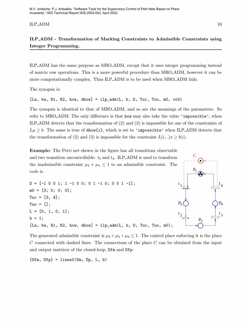
Example: The Petri net shown in the figure has all transitions observable

and two transition uncontrollable: t3 and t4. ILP ADM is used to transform

the inadmissible constraint µ2 + µ4 ≤ 1 to an admissible constraint. Thecode is

D = [-1 0 0 1; 1 -1 0 0; 0 1 -1 0; 0 0 1 -1];

m0 = [3; 0; 0; 0];

Tuc = [3, 4];

Tuo = [];

L = [0, 1, 0, 1];

b = 1;

[La, ba, R1, R2, how, dhow] = ilp_adm(L, b, D, Tuc, Tuo, m0);

C

p42p

3

3

tp

2t

1t 4t

1p

The generated admissible constraint is µ2+µ3+µ4 ≤ 1. The control place enforcing it is the placeC connected with dashed lines. The connections of the place C can be obtained from the input

and output matrices of the closed-loop, Dfm and Dfp:

[Dfm, Dfp] = linenf(Dm, Dp, L, b)


LINENF 11

LINENF - Linear Constraint Enforcement in Petri Nets

Description: LINENF enforces linear constraints of the form

Lµ+ Fq + Cv ≤ b (5)

where µ is the marking, q the firing vector, and v the Parikh vector (for all i, vi is the number of

firings of ti since the initialization of the system). The use of the constraints involving µ and q has

been described in [8]. The constraints Cv ≤ b can be used to describe fairness constraints (e.g. v3−v1 ≤ 0 specifies that t1 should fire at least as often as t3). When the PN has uncontrollable and/orunobservable transitions, the function uses PN transformations and MRO ADM and ILP ADM to

transform the constraints to admissible constraints.

The function operates as follows. In the case of PNs with no uncontrollable and unobservable

transitions, the input and output matrices of the supervisor enforcing (5) are:

D−c = max(0, LDp + C,F ) (6)

D+c = max(0, F −max(0, LDp + C))−min(0, LDp + C) (7)

where max(A,B,C, . . .) is the matrix X of elements xi,j = max(ai,j , bi,j, ci,j , . . .), min(A,B,C, . . .)

is similarly defined, and Dp is the incidence matrix of the plant PN. (Note that enforcing Cv ≤ bonly involves adding the rows of −C as rows to the incidence matrix.)

In the case of PNs with uncontrollable and/or unobservable transitions, the constraints (5) are

transformed to marking constraints. The Parikh vector constraints are transformed as follows.

Given a constraint

lTµ+ fT q + cT v ≤ d (8)

for each transition ti with vi 6= 0 a new place p′′i is generated, such that •p′′i = ti and p′′i • = ∅. Theneach civi with ci 6= 0 is replaced by ciµ(p′′i ).

The firing vector constraints are transformed using the indirect realization (section 7.2.2. in [8]).

In this approach, given a constraint

lTµ+ fT q ≤ d (9)

for each transition with fi > 0 a new place p′i and a new uncontrollable transition t

′i are added.

Then (9) is transformed into a marking inequality. The transformation employed by LINENF is

different from the one suggested in [8]. Thus, let g = lTD−p . If fi > 0, the term fiqi is replaced by(fi + gi)µ(p

′i); else the term fiqi is deleted. Adding the gi term allows LINENF to be effective on

coupled constraints.

LINENF does for each constraint of (5) the operations above. Such a transformed marking con-

straint is further transformed to be admissible. Then, it is enforced in the transformed Petri net.


LINENF 12

By collapsing the controlled net back to the original Petri net, the connections of the control place

in the original net are obtained. The theoretical background of the algorithm can be found in [2].

Synopsis:

[Dfm, Dfp, ms0] = linenf(pn, L, b, F, C)

[Dfm, Dfp, ms0, how, dhow] = linenf(Dm, Dp, L, b, m0, F, C, Tuc, Tuo)

where unnecessary arguments can be omitted or set to []. The notation is as follows:

• pn is a Petri net object.

• Dm and Dp are the input and output matrices of the plant Petri net.

• Dfm and Dfp are the input and output matrices of the controlled net. The last rows are therows of the control places.

• m0 is the initial marking. Use m0 = [] if the initial marking is not of interest.

• ms0 is the initial marking of the controlled net. If m0 = [], ms0 is set to an empty vector.

• Tuc and Tuo specify the set of uncontrollable and unobservable transitions, respectively. Forinstance, Tuc = [2, 3] and Tuo = 3 specify that t2, t3 are uncontrollable and t3 is unob-

servable, where ti stands for the transition corresponding to the i-th column of the incidence

matrix. Note that in the LINENF convention, a transition may be unobservable and yet

controllable.

• how is ’ok’ if all constraints have been successfully enforced, ’not solved’ if it failed withoutdetecting that the system of constraints cannot be enforced, and ’impossible’ if one of the

constraints cannot be enforced.

• dhow{i} reports the status of each constraint. Thus dhow{i} is ’ok’ if the constraint i hasbeen successfully enforced, ’impossible’ if LINENF detected that the constraint cannot be

enforced, and ’not solved’ otherwise.

It may be the case that we want to use the initial marking as a parameter for the marking of the

control places. Then the following format is useful:

[Dfm, Dfp, ms0, how, dhow, Lf, Cf, bf] = linenf(pn, L, b, F, C)

[Dfm, Dfp, ms0, how, dhow, Lf, Cf, bf] = linenf(Dm, Dp, L, b, m0, F, C, Tuc, Tuo)

In this format the initial marking of the control places can be obtained as bf − Lf*m0. Additionally,Cf allows us to specify the “invariant” enforced by the control places:

Lfµ+ Cfv + µc = bf (10)


LINENF 13

where µc is the marking of the control places.

Example: The Petri net shown in the figure has all transitions controllable and two transition

unobservable: t1 and t2. LINENF is used to transform the inadmissible constraint v1 − v2 ≤ 2 toan admissible constraint, and to enforce the admissible constraint on the Petri net. The code is

D = [-1 -1 1 1; 1 0 -1 0; 0 1 0 -1];

m0 = [2 0 0]’;

Tuc = []; Tuo = [];

L = []; F = [];

C = [1 -1 0 0]; b = 2;

[Dm, Dp] = d2dd(D);

pn = getpn(Dm, Dp, Tuc, Tuo, m0);

[Dfm,Dfp,ms0,how,dhow,Lf,Cf.bf] = linenf(pn, L, b, F, C);

C

t 43t

2t1t

3pp2 1p

The generated admissible constraint has the form Lfµ+ Cfv ≤ bf , and is µ1 + 2µ3 + v1 − v2 ≤ 2.The control place enforcing it is the place C connected with dashed lines. The connections of the

place C are obtained from the input and output matrices of the closed-loop, Dfm and Dfp.

Programs testing the linear constraint enforcement

A number of Matlab scripts with test data have also been generated. Most tests are taken from

the examples in [8]. The tests have been put together in the script LINTST.


ISADM 14

ISADM - Checks whether a set of constraints is admissible

Given a plant Petri net, it is important to answer the question of whether a set of desirable

constraints on the operation of the net is admissible. A constraint is said to be admissible if its

enforcement under the assumption that all transitions are controllable and observable does not

attempt to inhibit uncontrollable transitions and does not detect unobservable transitions. The

admissibility of a set of constraints is typically dependent on the initial marking. Therefore, when

the initial marking is given, the function performs a reachability analysis to establish whether the

constraints are admissible.

The synopsis is

[o] = isadm(pnobj, L, b)

[o] = isadm(pnobj, L, F, b)

[o] = isadm(pnobj, L, F, C, b)

where

• pnobj is a Petri net object (obtained with GETPN) describing the plant.

• L, F, C and b are the parameters of the constraints:

Lµ+ Fq + Cv ≤ b (11)

• The output o is a vector evaluating the admissibility of each constraint of the set of constraintsas follows:

1. o(i) = 1 if constraint i is admissible

2. o(i) = 0 if constraint i is inadmissible

3. o(i) = -1 if the admissibility of constraint i could not be decided.

For the reachability analysis, the function computes the coverability graph of the closed-loop Petri

net. The closed-loop Petri net is the plant Petri net connected to the supervisor enforcing (11),

obtained under the assumption that all transitions are controllable and observable. The function

may not be able to decide admissibility only if the supervisor part of the closed-loop Petri net is

unbounded.

Structural analysis with ISADM

When no initial marking is specified in pnobj or when b = [], the function performs a structural

analysis to determine whether the constraint is admissible. In this case the output should be

interpreted as follows:


ISADM 15

1. if o(i) = 1, then the constraint i is admissible for all initial markings satisfying the con-

straints.

2. if o(i) = 0, then initial markings may exist such that constraint i is inadmissible.

The structural analysis implementation in ISADM is very fast, however, not as powerful as reach-

ability analysis.

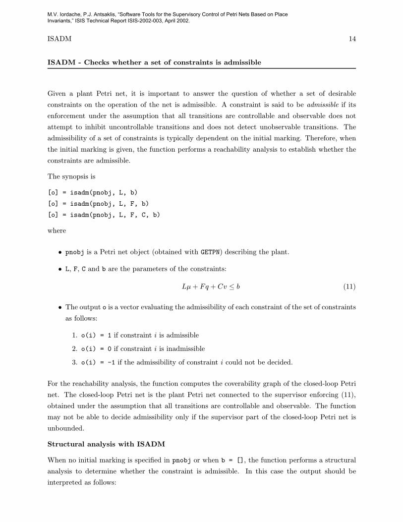
Example: Consider Petri net below modeling the three-tank probem from [8]. All transitions are

observable, but only t1, t2, and t3 are controllable. The following code can be used to verify that

the constraint

2q1 + µ6 + µ9 − 2µ3 ≤ 2

is admissible, and that

µ2 + µ5 + µ8 ≥ 3

is inadmissible.

D1 = [ 1 -1 0 0; -1 1 -1 1; 0 0 1 -1;];

D = [zeros(9,3) [D1; zeros(6,4)] [zeros(3,4); D1; zeros(3,4)] [zeros(6,4); D1]];

Tuc = [4:15]; Tuo = [];

[Dm, Dp] = d2dd(D);

m0 = zeros(9,1); m0([2 5 8]) = 1;

pn = getpn(Dm, Dp, Tuc, Tuo, m0);

F = [2, zeros(1,14); zeros(1,15)];

L = zeros(2,9);

L(1,[3,6,9]) = [-2, 1, 1];

L(2,[2,5,8]) = -1;

b = [2; -3];

[v] = isadm(pn, L, F, b);

13

t 14 t 15

t 12

p52 8

t 5

t 6

pt

t8t

11t10

p

9t4t

7t

6p 9p3p

7p4p1p

3t2t1t

Note that structural analysis does not detect that the first constraint is admissible (at the given

initial marking):

[v] = isadm(pn, L, F, []);

returns v = [0, 0].

Test file

ISADMTST is a script containing examples for ISADM.


16

Invariant Computation

We may be interested to find the place or transition invariants of a Petri net. Matlab provides

the function null, which finds a base of the null space of a matrix. For instance, if we desire to

compute a base of the invariants satisfying Ax = 0 for some matrix A, the synopsis is

V = null(A,’r’)

Then any invariant can be expressed as:

x = V*a

where a is a column vector. The second argument ’r’ insures that V is an integer matrix (when A

is also).

Example: In the Petri net below, all place invariants are of the form αv, α ∈ R, for

v = [ 1 1 1 ]

and all transition invariants are a linear combination (with real coefficients) of v1, v2, and v3 below:

v1 = [ 1 1 1 0 0 ]T

v2 = [ −1 −2 0 1 0 ]T

v3 = [ 1 2 0 0 1 ]T

The code below obtains this result:

D = [-1 1 0 1 -1; -1 0 1 -1 1; 2 -1 -1 0 0];

% Place invariant computation

v = null(D’,’r’);

% Transition invariant computation

v = null(D, ’r’); p3

1

5

p p

t

2

4t

1tt 2 t 32


INVAR 17

Positive Invariant Computation

Problem Statement. We say that x is a positive invariant of M if Mx = 0, x ≥ 0, and x 6= 0.Given a matrix M , we are looking to find a number of vectors v1, v2, . . . vm such that

Mx = 0 and x ≥ 0⇐⇒ x =∑αivi and αi ≥ 0 (12)

The vectors v1, v2, . . . vm satisfying (12) obviously satisfy: vi ≥ 0 for i = 1 . . . m. The support ofa vector x is the set of indices j for which x(j) 6= 0; we denote by ‖x‖ the support x. We considerinvariants which are not equal to the null vector. For such invariants we say that x is a minimal

support invariant if x is an invariant and there is no invariant y such that ‖y‖ ⊂ ‖x‖.

It can be noticed that we can solve the problem of (12) if we take v1, . . . vm positive invariants

with mimimal support, such that all supports of the minimal support positive invariants appear in

‖v1‖, . . . ‖vm‖, and ‖v1‖, . . . ‖vm‖ are distinct. Indeed, the ⇐ direction of the proof is obvious,while the ⇒ direction is as follows. To find the coefficients αi, we first set them to 0. Next, notethat a positive invariant x satisfies that there is vi such that ‖vi‖ ⊆ ‖x‖. Then we set αi to thelargest real such that x−αivi ≥ 0. Then let x2 = x−αivi; if x2 6= 0, x2 is a positive invariant, andso we apply to x2 the same procedure as for x, in order to set a new coefficient αi. Eventually we

get to an xn such that xn = 0. At that time we know that x =∑αivi.

Furthermore it can also be noticed that we have the minimum number of vectors v1 . . . vm solving

(12) if we take them the minimal support positive invariants, as above.

Computational Complexity. The problem of finding the positive invariants may not be easy

to solve. It is known that a matrix may have an exponential number of positive invariants with

minimal (and distinct) support. For instance consider the matrix

N = [v1, v2, . . . vn] (13)

Assume that there is a single minimal support of positive invariants; so there is a positive invariant

α 6= 0 having that support, that is:

α1v1 + α2v2 + . . . αnvn = 0 (14)

and αi ≥ 0, for all i = 1 . . . n. Then notice that the matrix

M = [v1, v2, . . . vn, v1, v2, . . . vn] (15)

has 2n distinct minimal supports of positive invariants! This proves that the number of minimal

supports of positive invariants of a matrix with n columns can be larger than 2bn/2c.

Implementation. The use of the function INVAR is proposed. This is a slight modification of

INVAR1, which has been developed in our group in the past. The modification is that INVAR


INVAR 18

insures that the intermediary rows are integer. This solves the problems of INVAR1 which are

known to the authors. INVAR1 is based on an algorithm by Martinez and Silva [7].

Synopsis:

C = invar(A)

The function computes a set of positive invariants with minimal support, and stores them as

columns in C. Unlike INVAR1, invariants satisfying Ax = 0 instead of xTA = 0 are computed.

Example: In the Petri net below, all positive place invariants are of the form αv, α ∈ R+, for

v = [ 1 1 1 ]

and all positive transition invariants are given by the v1 . . . v4 below:

v1 = [ 1 1 1 0 0 ]T

v2 = [ 1 2 0 1 0 ]T

v3 = [ 1 2 0 0 1 ]T

v4 = [ 0 0 0 1 1 ]T

The code below obtains this result:

D = [-1 1 0 1 -1; -1 0 1 -1 1; 2 -1 -1 0 0];

% Place invariant computation

v = invar(D’);

% Transition invariant computation

v = invar(D); p3

1

5

p p

t

2

4t

1tt 2 t 32


DP 19

DP - Deadlock Prevention and Liveness Enforcement

Description: This function can be used to generate deadlock prevention supervisors, liveness

enforcing supervisors, and T -liveness enforcing supervisors.

Deadlock is the state of a system that has become permanently blocked.

Deadlock Prevention means to prevent reaching a state of total deadlock.

Liveness Enforcement means to ensure that no local deadlocks occur. In the Petri net termi-

nology, this means ensuring that all transitions are live.

T -liveness Enforcement means to ensure that no deadlocks occur in the part of the system

characterized by the set T . In the Petri net terminology, this means ensuring that all transi-

tions in the set T are live.

DP generates by default deadlock prevention supervisors. They typically enforce liveness or T -

liveness (for the largest possible set T ). Options can be set to force DP generate supervisors

guaranteed to enforce liveness or T -liveness, for arbitrary sets T . However, in the default mode DP

is most likely to converge.

The supervisors are defined as follows. Given a Petri net, DP generates the marking constraints

Lµ ≥ B and L0µ ≥ B0, such that when the Petri net is supervised according to Lµ ≥ B, it isdeadlock-free/live/T -live for all initial markings µ0 satisfying Lµ0 ≥ B and L0µ0 ≥ B0. Further-more, the constraints Lµ ≥ B are guaranteed to be admissible.

Synopsis: The following format can be used:

[L, B, L0, B0, how] = dp(pn, T, L, B, L0, B0, opt)

where the simpler formats below are also available:

[L, B, L0, B0, how] = dp(pn)

[L, B, L0, B0, how] = dp(pn, T)

[L, B, L0, B0, how] = dp(pn, T, L, B)

[L, B, L0, B0, how] = dp(pn, T, L, B, L0, B0)

Alternative formats which do not refer to Petri net objects are also available, and they are described

in the help lines. The significance of the arguments is as follows:

• pn is a Petri net object created by GETPN. The initial marking (if any) of pn is ignored, asDP relies on structural net analysis.


DP 20

• T is the set of transitions T for T -liveness enforcement. To omit T , replace it with the emptyvector []. The default value of T is the set of transitions of the Petri net.

• L and B are the matrices L and B produced by the procedure. If their initial value is notempty, they can be given as input arguments. Nonempty initial L and B are interpreted as

additional constraints Lµ ≥ B to be enforced on the Petri net. The inputs L and B can beomitted by replacing each of them with the empty vector [].

• L0 and B0 are the matrices L0 and B0 produced by the procedure. If their initial value is notempty, they can be given as input arguments. Nonempty initial L0 and B0 are interpreted

as constraints that all reachable markings satisfy, if the initial marking satisfies them. Initial

L0 and B0 can be used to help the procedure converge. The inputs L0 and B can be omitted

by replacing each of them with the empty vector [].

• opt is the options input. The options are of the form opt = 8l + 4k + 2i+ j, where:

– j = (0)/1 turns (OFF)/ON the verbose mode.

– k = (0)/1 turns (OFF)/ON printing log files. In the default mode, two files dp.log and

dp.dat are generated in the current directory. The file dp.log describes the operation

of DP; upon termination, DP writes at the end of dp.log the constraints defining the

supervisor, and comments on the significance of the supervisor. The file dp.dat describes

the intermediary Petri nets generated during the operation of DP.

– l = 0/(1) selects between deadlock prevention (default) and liveness or T -liveness en-

forcement. When l = 1, liveness enforcement is performed when the input argument T

is the empty vector. For T -liveness enforcement, set l = 1 and the argument T to the

set T .

• how is either of the strings ’ok’, ’failed’ or ’impossible’.

– The string ’ok’ corresponds to a successful operation of DP, in the sense that deadlock is

prevented, or that the supervisor is guaranteed to enforce at least Tx-liveness (where the

set Tx is reported in dp.log, if different from T , in the case of T -liveness enforcement,

or if not equal to the total set of transitions, in the case of liveness enforcement).

– The string ’failed’ corresponds to DP failing to generate a supervisor. When this

happens, it is possible that no solution exists.

– The string ’impossible’ corresponds to DP detecting that deadlock prevention is im-

possible. (Note that liveness and T -liveness enforcement imply deadlock prevention.)

Algorithm: DP relies on an iterative procedure. At every iteration a class of siphons of the net are

computed and controlled. The procedure is not guaranteed to terminate. The procedure employed

in DP is a combination of the procedures presented in [3, 4, 1, 5].


DP 21

Examples: The Petri net below has controllable transitions and an unobservable transition: t1.

The following code can be used to run the deadlock prevention procedure and to run the liveness

enforcement procedure:

D = [-1 1 0; -1 0 1; 2 -1 -1];

[Dm, Dp] = d2dd(D);

Tuc = []; Tuo = 1;

pn = getpn(Dm, Dp, Tuc, Tuo);

% Run the deadlock prevention procedure

[L, b, L0, b0, how] = dp(pn);

% Run the liveness enforcement procedure

opt = 15;

[L, b, L0, b0, how] = dp(pn, [], [], [], [], [], opt);

31 t2

p

t

p

p3

1

t

2

2

Let T = {t4, t5}. To enforce T -liveness in the Petri net at theright, the following code can be used:

D = [-1 1 0 1 -1; -1 0 1 -1 1; 1 -2 -2 0 0];

T = [4, 5];

pn = getpn(D);

opt = 15;

[L, b, L0, b0, how] = dp(pn, T, [], [], [], [], opt);

p3

1

5

p p2

t

4t

1tt 2 t 3

2 2

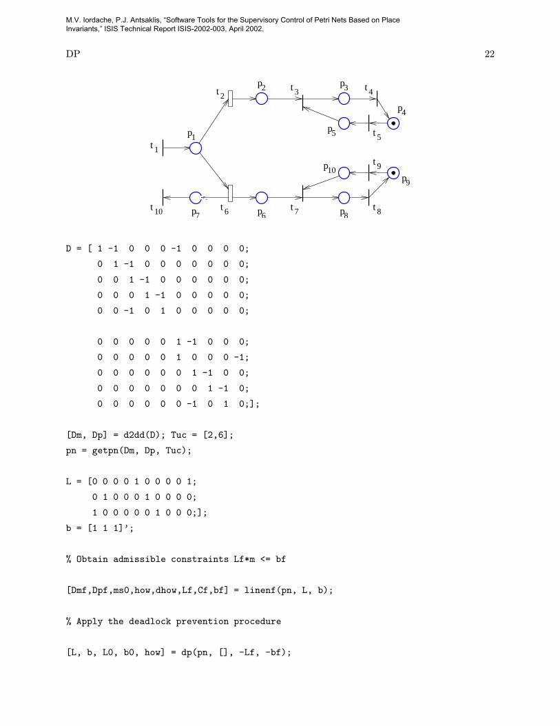
The next example is from [8], pp. 122-129. The following code shows how to obtain the solution

using LINENF and DP. The problem is as follows. The following Petri net has observable transitions

and two uncontrollable transitions: t2 and t6. It is desired to enforce the constraints:

µ5 + µ10 ≤ 1

µ2 + µ6 ≤ 1

µ1 + µ7 ≤ 1

The constraints are inadmissible, and so are transormed to admissible constraints using LINENF.

As the closed-loop is blocking, DP is used to add new constraints such that the closed-loop is

deadlock-free. The code follows.


DP 22

p6p7 p8

5

p10

10

p

4

p

p

3p

9

t

9t

8t6t 7t

5t

4t3t2t

1t1p

p2

D = [ 1 -1 0 0 0 -1 0 0 0 0;

0 1 -1 0 0 0 0 0 0 0;

0 0 1 -1 0 0 0 0 0 0;

0 0 0 1 -1 0 0 0 0 0;

0 0 -1 0 1 0 0 0 0 0;

0 0 0 0 0 1 -1 0 0 0;

0 0 0 0 0 1 0 0 0 -1;

0 0 0 0 0 0 1 -1 0 0;

0 0 0 0 0 0 0 1 -1 0;

0 0 0 0 0 0 -1 0 1 0;];

[Dm, Dp] = d2dd(D); Tuc = [2,6];

pn = getpn(Dm, Dp, Tuc);

L = [0 0 0 0 1 0 0 0 0 1;

0 1 0 0 0 1 0 0 0 0;

1 0 0 0 0 0 1 0 0 0;];

b = [1 1 1]’;

% Obtain admissible constraints Lf*m <= bf

[Dmf,Dpf,ms0,how,dhow,Lf,Cf,bf] = linenf(pn, L, b);

% Apply the deadlock prevention procedure

[L, b, L0, b0, how] = dp(pn, [], -Lf, -bf);


DP 23

Demonstration Scripts: DPDEM and LEDEM are simple demonstration scripts for deadlock pre-

vention and (T -)liveness enforcement, respectively.


24

Complete List of Functions and Scripts

ACTN - Computation of a maximal active subnet.

ADMCON - Transformation to admissible constraints.

AR2PN - Conversion from net representation to incidence matrix representation.

ASIPH - Computation of minimal or minimal active siphons of a Petri net.

AVPR - Converts vectors to strings.

CHK CONS - Checks constraint consistency.

CHK CON2 - Checks constraint consistency.

CHK DATA - Checks data consistency.

D2DD - Transforms an incidence matrix D into a input and output matrix pair (D−, D+).

DISGRAPH - Text display of coverability graph objects.

DP - Generates a supervisor for deadlock prevention, liveness enforcement, or T -liveness enforce-

ment.

DPDEM - Demonstration program for DP.

FVPR - Coverts vectors to strings.

GCDV - Greatest common divisor of the elements of a vector/matrix.

GETPN - Creates a Petri net object.

GRP - Checks a pattern occurrence in a string.

ILP ADM - Transformation to admissible constraints based on integer programming.

INVAR - Computes a basis of positive invariants of a Petri net.

IP SOLVE - Mixed integer program solver based on LP SOLVE.

ISADM - Checks the admissibility of a set of constraints.

ISADMTST - Demonstration program for ISADM.

LEDEM - Demonstration program for DP.

LINENF - Enforces linear constraints on a Petri net.


25

LINTST - Demonstration program for LINENF.

MRO ADM - Transformation to admissible constraints based on matrix row operations.

MSPLIT - Transformation to partially ordinary nets.

NLTRANS - Computes transitions which cannot be made live.

PN2ACPN - Transformation to asymmetric-choice nets.

PN2AR - Conversion from incidence matrix representation to net representation.

PNCGRAPH - Computes the coverability/reachability graph.

PNPRED - Subroutine of PNCGRAPH.

REDUCE - Removes redundant constraints.

SUPERVIS - Enforces linear constraints in fully controllable and observable Petri nets.

TACTN - Computation of a T -minimal active subnet.

TS ADM - Subroutine of ISADM.


26

References

[1] M. V. Iordache and P. J. Antsaklis. T -liveness enforcement in Petri nets based on structuralnet properties. In Proceedings of the 40th IEEE International Conference on Decision and

Control., December 2001.

[2] M. V. Iordache and P. J. Antsaklis. Synthesis of supervisors enforcing general linear vector

constraints in Petri nets. In Proceedings of the 2002 American Control Conference, pages

154–159, May 2002.

[3] M. V. Iordache, J. O. Moody, and P. J. Antsaklis. A method for the synthesis of deadlock

prevention controllers in systems modeled by Petri nets. In Proceedings of the 2000 American

Control Conference, pages 3167–3171, June 2000.

[4] M. V. Iordache, J. O. Moody, and P. J. Antsaklis. A method for the synthesis of liveness

enforcing supervisors in Petri nets. In Proceedings of the 2001 American Control Conference,

pages 4943–4948, June 2001.

[5] M. V. Iordache, J. O. Moody, and P. J. Antsaklis. Synthesis of deadlock prevention supervisors

using Petri nets. IEEE Transactions on Robotics and Automation, 18(1):59–68, February 2002.

[6] M. Jantzen and R. Valk. Formal properties of place/transition nets. In Brauer, W., editor,

Lecture Notes in Computer Science: Net Theory and Applications, Proc. of the Advanced

Course on General Net Theory of Processes and Systems, Hamburg, 1979, volume 84, pages

165–212, Berlin, Heidelberg, New York, 1980. Springer-Verlag.

[7] J. Martinez and M. Silva Suarez. A simple and fast algorithm to obtain all invariants of

a generalized petri net. In Girault, C. and Reisig, W., editors, Informatik-Fachberichte 52:

Application and Theory of Petri Nets: Selected Papers from the First and Second European

Workshop on Application and Theory of Petri Nets, Strasbourg, Sep. 23-26, 1980, Bad Honnef,

Sep. 28-30, 1981, pages 301–310. Springer-Verlag, 1982.

[8] J. O. Moody and P. J. Antsaklis. Supervisory Control of Discrete Event Systems Using Petri

Nets. Kluwer Academic Publishers, 1998.

[9] W. Reisig. Petri Nets, volume 4 of EATCS Monographs on Theoretical Computer Science.

Springer-Verlag, 1985.

[10] E. Yamalidou, J. O. Moody, P. J. Antsaklis, and M. D. Lemmon. Feedback control of Petri

nets based on place invariants. Automatica, 32(1):15–28, January 1996.


software tools for the supervisory control of petri nets based on place invariants

Documents