software engineering - kaistspiral.kaist.ac.kr/wp/2015springcs550/download/2015springcs550/07... ·...

Software Engineering(CS550)

Jongmoon Baik

Estimation w/ COCOMOII

2

WHO SANG COCOMO?

• The Beach Boys [1988]

• “KoKoMo” Aruba, Jamaica,ooo I wanna take youTo Bermuda, Bahama,come on, pretty mamaKey Largo, Montego, baby why don't we go jamaicaOff the Florida Keys there's a place called KokomoThat's where you want to go to get away from it allBodies in the sandTropical drink melting in your handWe'll be falling in love to the rhythm of a steel drum bandDown in Kokomo……………………..………………………..

3

What is COCOMO?

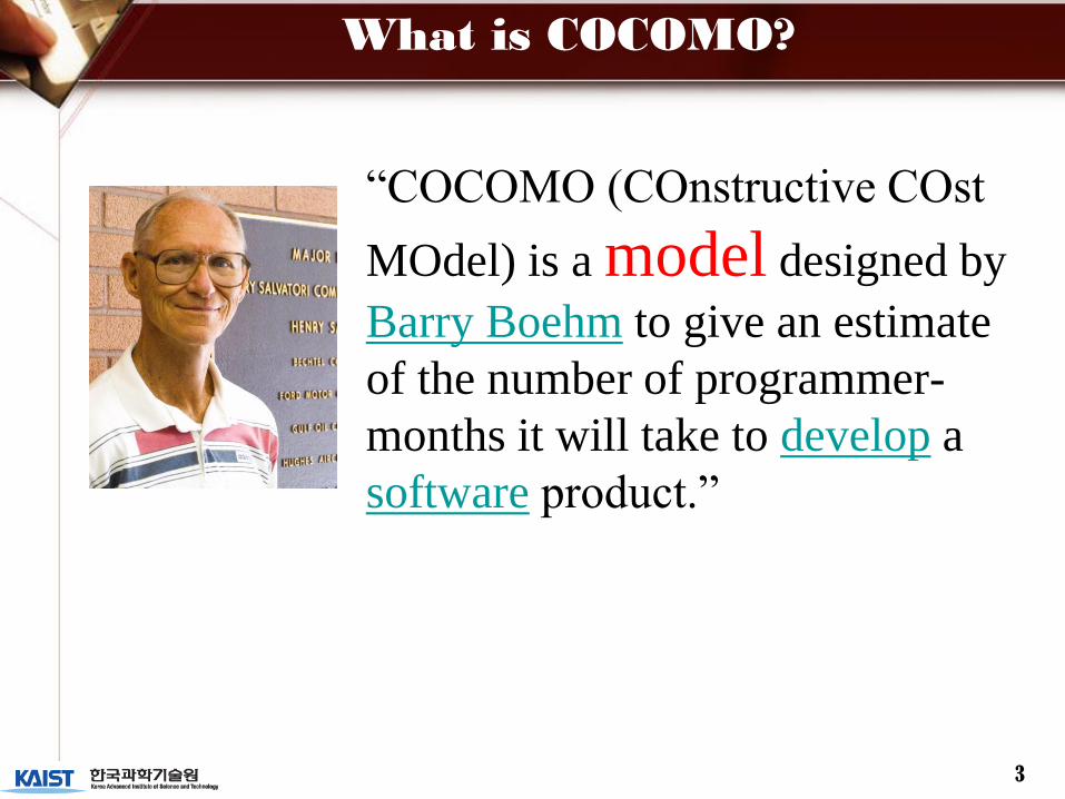
“COCOMO (COnstructive COst

MOdel) is a model designed by

Barry Boehm to give an estimate

of the number of programmer-

months it will take to develop a

software product.”

http://en.wikipedia.org/wiki/Barry_Boehm

http://en.wikipedia.org/wiki/Software_development_process

http://en.wikipedia.org/wiki/Computer_software

4

COCOMO II Overview - I

Software product size estimate

Software product, process,computer, and personnel attributes

Software reuse, maintenance,and increment parameters

Software organization’sproject data

Software development,maintenance cost andschedule estimates

Cost, schedule distributionby phase, activity, increment

COCOMO recalibratedto organization’sdata

COCOMO II

5

COCOMO II Overview - II

• Open interfaces and internals– Published in Software Cost Estimation with COCOMO II, Boehm et.

al., 2000

• COCOMO – Software Engineering Economics , Boehm, 1981

• Numerous Implementation, Calibrations, Extensions– Incremental Development, Ada, new environment technology

– Arguably the most frequently-used software cost model worldwide

6

List of COCOMO II

Packages• USC COCOMO II.2000 - USC

• Costar – Softstar Systems

• ESTIMATE PROFESSIONAL – SPC

• CostXpert – Marotz

• Partial List of COCOMO Packages (STSC,

1993)

– CB COCOMO, GECOMO Plus, COCOMOID,

GHL COCOMO, COCOMO1, REVIC, CoCoPro,

SECOMO, COSTAR, SWAN, COSTMODL

7

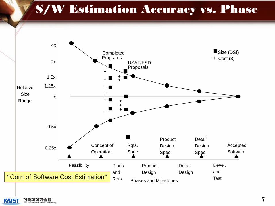
S/W Estimation Accuracy vs. Phase

Plans

and

Rqts.

Devel.

and

TestPhases and Milestones

Size (DSI)

+ Cost ($)

+

+

++++

+

+

++

+++

4x

2x

1.5x

1.25x

x

0.25x

0.5x

Relative

Size

Range

CompletedPrograms

USAF/ESDProposals

Feasibility Product

Design

Detail

Design

Concept of

Operation

Rqts.

Spec.

Product

Design

Spec.

Detail

Design

Spec.

Accepted

Software

“Corn of Software Cost Estimation”

8

MBASE/UP Anchor Point Milestones

App.

Compos.Inception Elaboration, Construction

LCO,

LCA

IOC

Waterfall

Rqts. Prod. Des.

LCA

Development

LCO

Sys

Devel

IOC

Transition

SRR PDR

Construction

SAT

Trans.Inception

PhaseElaboration

9

Application Composition Model

• Challenge:

– Modeling rapid application composition with

graphical user interface (GUI) builders, client-

server support, object-libraries, etc.

• Responses:

– Application-Point Sizing and Costing Model

– Reporting estimate ranges rather than point

estimate

10

Application Point Estimation Procedure

Element Type Complexity-WeightSimple Medium Difficult

Screen 1 2 3Report 2 5 83GL Component 10

Step 1: Assess Element-Counts: estimate the number of screens, reports, and 3GL components that will comprise this

application. Assume the standard definitions of these elements in your ICASE environment.

Step 2: Classify each element instance into simple, medium and difficult complexity levels depending on values of

characteristic dimensions. Use the following scheme:

For Screens For Reports

# and source of data tables # and source of data tables

Number of

Views

Contained

Total < 4

(<2 srvr, <3

clnt)

Total <8

(<3 srvr, 3 -

5 clnt)

Total 8+

(>3 srvr, >5

clnt)

Number

of Sections

Contained

Total < 4

(<2 srvr, <3

clnt)

Total <8

(<3 srvr, 3 -

5 clnt)

Total 8+

(>3 srvr, >5

clnt)

<3 simple simple medium 0 or 1 simple simple medium

3-7 simple medium difficult 2 or 3 simple medium difficult

>8 medium difficult difficult 4+ medium difficult difficult

Step 3: Weigh the number in each cell using the following scheme. The weights reflect the relative effort required to

implement an instance of that complexity level.

Step 4: Determine Application-Points: add all the weighted element instances to get one number, the Application-Point count.

Step 5: Estimate percentage of reuse you expect to be achieved in this project. Compute the New Application Points to be

developed NAP =(Application-Points) (100-%reuse) / 100.

Step 6: Determine a productivity rate, PROD=NAP/person-month, from the following scheme:

Developer's experience and capability Very Low Low Nominal High Very High

ICASE maturity and capability Very Low Low Nominal High Very High

PROD 4 7 13 25 50

Step 7: Compute the estimated person-months: PM=NAP/PROD.

11

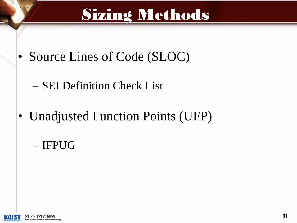
Sizing Methods

• Source Lines of Code (SLOC)

– SEI Definition Check List

• Unadjusted Function Points (UFP)

– IFPUG

12

Source Lines of Code

• Best Source : Historical data form previous projects

• Expert-Judged Lines of Code

• Expressed in thousands of source lines of code

(KSLOC)

• Difficult Definition – Different Languages

• COCOMO II uses Logical Source Statement– SEI Source Lines of Code Check List

– Excludes COTS, GFS, other products, language support libraries and

operating systems, or other commercial libraries

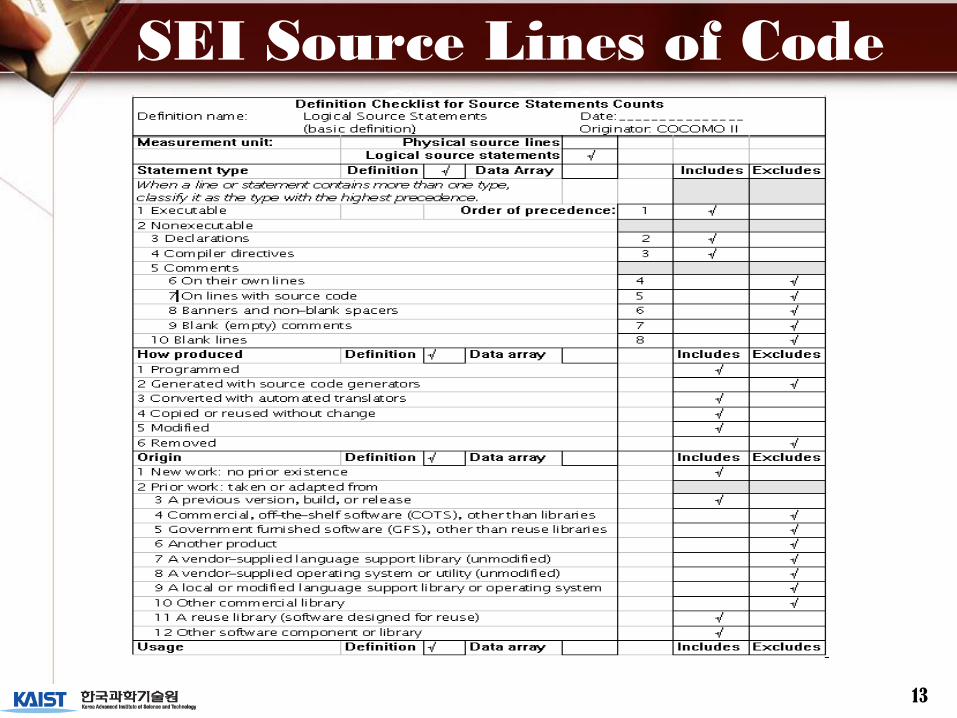
13

SEI Source Lines of Code

Checklist

14

Unadjusted Function Points

- I• Based on the amount of functionality in a software

project and a set of individual project factors.

• Useful since they are based on information that is available early in the project life-cycle.

• Measure a software project by quantifying the information processing functionality associated with major external data or control input, output, or file types.

15

Unadjusted Function Points

- IIStep 1. Determine function counts by type. The unadjusted function point counts should be counted by a lead technical person based on

information in the software requirements and design documents. The number of each the five user function types should be counted

(Internal Logical File (ILF), External Interface File (EIF), External Input (EI), External Output (EO), and External Inquiry (EQ)).

Step 2. Determine complexity-level function counts. Classify each function count into Low, Average, and High complexity levels

depending on the number of data element types contained and the number of file types reference. Use the following scheme.

For ILF and EIF For EO and EQ For EI

Data Elements Data Elements Data Elements Record Elements 1-19 20-50 51+

File Types

1-5 6-19 20+

File Types

1-4 5-15 16+

1 Low Low Avg 0 or 1 Low Low Avg 0 or 1 Low Low Avg

2-5 Low Avg High 2-3 Low Avg High 2-3 Low Avg High

6+ Avg High High 4+ Avg High High 4+ Avg High High

Step 3. Apply complexity weights. Weight the number in each cell using the following scheme. The weight reflect the relative value of

the function to the user.

Complexity Weight Function Type

Low Average High

Internal Logical File (ILF) 7 10 15

External Interface Files (EIF) 5 7 10

External Inputs (EI) 3 4 6

External Outputs 4 5 7

External Inquiries 3 4 6

Step 4. Compute Unadjusted Function Points. Add all the weight functions counts to get one number, the Unadjusted Function Points.

16

Relating UFPs to SLOC

• USC-COCOMO II– Use conversion table (Backfiring) to convert UFPS into

equivalent SLOC

– Support 41 implementation languages and USR1-5 for accommodation of user’s additional implementation languages

– Additional Ratios and Updates : http://www.spr.com/library/0Langtbl.htm

Language SLOC/UFP Language SLOC/UFP

Access 38 Ada 83 71 Ada 95 49

.

.

.

.

.

.

.

Jovial 107 Lisp 64 Machine Code 640

.

. USR_1 1 USR_2 1

.

.

.

17

Exercise - I

• Suppose you are developing a stand-alone

application composed of 2 modules for a client

– Module 1 written in C

• FP multiplier C 128

– Module 2 written in C++

• FP multiplier C++ 53

• Determine UFP’s and equivalent SLOC

18

Information on Two Modules


Low Average High







Low Average High






Module 1

Module 2

FP default weight values

19

Early Design & Post-Architecture Models

• Early Design Model [6 EMs]:

• Post Architecture Model [16 EMs]:*Exclude SCED driver

EMs: Effort multipliers to reflect characteristics of particular software under development

A : Multiplicative calibration variableE : Captures relative (Economies/Diseconomies of scale)SF: Scale Factors

A = 2.94 B = 0.91

C = 3.67 D = 0.28

20

Scale Factors & Cost

Drivers• Project Level – 5 Scale Factors

– Used for both ED & PA models

• Early Design – 7 Cost Drivers

• Post Architecture – 17 Cost Drivers

– Product, Platform, Personnel, Project

21

Project Scale Factors - I

• Relative economies or diseconomies of scale– E < 1.0 : economies of scale

• Productivity increase as the project size increase

• Achieved via project specific tools (e.g., simulation, testbed)

– E = 1.0 : balance

• Linear model : often used for cost estimation of small projects

– E > 1.0 : diseconomies of scale

• Main factors : growth of interpersonal communication overhead and growth of large-system overhead

22

Project Scale Factors - II

Scale Factors (SFi )

Very Low

Low

Nominal

High

Very High

Extra High

thoroughly

unprecedente

d

largely

unprecedente

d

somewhat

unprecedente

d

generally

familiar

largely

familiar

throughly

familiar PREC

6.20 4.96 3.72 2.48 1.24 0.00

rigorous

occasional

relaxation

some

relaxation

general

conformity

some

conformity

general goals FLEX

5.07 4.05 3.04 2.03 1.01 0.00

little (20%) some (40%) often (60%) generally(75

%)

mostly (90%) full (100%) RESL

7.07 5.65 4.24 2.83 1.41 0.00

very difficult

interactions

some difficult

interactions

basically

cooperative

interactions

largely

cooperative

highly

cooperative

seamless

interactions

TEAM

5.48 4.28 3.29 2.19 1.10 0.00

SW-CMM

Level 1

Lower

SW-CMM

Level 1

Upper

SW-CMM

Level 2

SW-CMM

Level 3

SW-CMM

Level 3

SW-CMM

Level 5

PMAT

Or the Estimated Process Maturity Level (EPML)

7.80 6.24 4.68 3.12 1.56 0.00

23

PMAT == EPML

• EPML (Equivalent Process Maturity Level)

24

PA Model – Product EMs

Effort Multiplier

Very Low

Low

Nominal

High

Very High

Extra High

slight inconven-

ience

low, easily

recoverable

losses

moderate, easily

recoverable

losses

high financial

loss

risk to human

life

RELY

0.82 0.92 1.00 1.10 1.26 n/a

DB bytes/Pgm

SLOC < 10

10 <= D/P < 100 100 <= D/P <

1000

D/P>=1000 DATA

n/a 0.90 1.00 1.14 1.28 n/a

none across project across program across product

line

across multiple

product lines RUSE

n/a 0.95 1.00 1.07 1.15 1.24

Many life-cycle

needs uncovered

Some life-cycle

needs

uncovered.

Right-sized to

life-cycle needs

Excessive for

life-cycle needs

Very excessive

for life-cycle

needs

DOCU

0.81 0.91 1.00 1.11 1.23 n/a

CPLX See CPLX table

0.73 0.87 1.00 1.17 1.34 1.74

25

PA Model - CPLX

Effort Multiplier

Control Operations Computational

Operations Device-dependent

Operations Data Management

Operations User Interface

Management

Operations Very Low Straight-line code with

a few non-nested structured

programming operators: DOs,

CASEs, IF-THEN-ELSEs. Simple

module composition via procedure calls or

simple scripts.

Evaluation of simple expressions: e.g.,

A=B+C*(D-E)

Simple read, write statements with simple

formats.

Simple arrays in main memory. Simple COTS-DB queries,

updates.

Simple input forms, report generators.

Low

… … … … …

Nominal

Mostly simple nesting.

Some intermodule

control. Decision

tables. Simple

callbacks or message

passing, including

middleware-supported

distributed processing

Use of standard math and

statistical routines.

Basic matrix/vector

operations.

I/O processing includes

device selection, status

checking and error

processing.

Multi-file input and

single file output.

Simple structural

changes, simple edits.

Complex COTS-DB

queries, updates.

Simple use of widget set.

High … … … … …

Very High … … … … …

Extra High Multiple resource scheduling with dynamically changing priorities. Microcode-level control. Distributed hard real-time control.

Difficult and unstructured numerical analysis: highly accurate analysis of noisy, stochastic data. Complex parallelization.

Device timing-dependent coding, micro-programmed operations. Performance-critical embedded systems.

Highly coupled, dynamic relational and object structures. Natural language data management.

Complex multimedia, virtual reality, natural language interface.

26

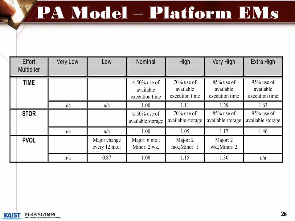
PA Model – Platform EMs

Effort Multiplier

Very Low

Low

Nominal

High

Very High

Extra High

50% use of

available

execution time

70% use of

available

execution time

85% use of

available

execution time

95% use of

available

execution time

TIME

n/a n/a 1.00 1.11 1.29 1.63

50% use of

available storage

70% use of

available storage

85% use of

available storage

95% use of

available storage STOR

n/a n/a 1.00 1.05 1.17 1.46

Major change

every 12 mo.;

Minor change

every 1 mo.

Major: 6 mo.;

Minor: 2 wk.

Major: 2

mo.;Minor: 1

wk.

Major: 2

wk.;Minor: 2

days

PVOL

n/a 0.87 1.00 1.15 1.30 n/a

27

PA Model – Personnel EMs

Effort Multiplier

Very Low

Low

Nominal

High

Very High

Extra High

15th percentile 35th percentile 55th percentile 75th percentile 90th percentile ACAP

1.42 1.19 1.00 0.85 0.71 n/a

15th percentile 35th percentile 55th percentile 75th percentile 90th percentile PCAP

1.34 1.15 1.00 0.88 0.76 n/a

48% / year 24% / year 12% / year 6% / year 3% / year PCON 1.29 1.12 1.00 0.90 0.81 n/a

<= 2 months 6 months 1 year 3 years 6 years APEX

1.22 1.10 1.00 0.88 0.81 n/a

<= 2 months 6 months 1 year 3 years 6 year LTEX

1.20 1.09 1.00 0.91 0.84 n/a

PLEX <= 2 months 6 months 1 year 3 years 6 year

1.19 1.09 1.00 0.91 0.85 n/a

28

PA Model – Project EMs

Effort Multiplier

Very Low

Low

Nominal

High

Very High

Extra High

edit, code, debug simple, frontend,

backend CASE,

little integration

basic life-cycle

tools,

moderately

integrated

strong, mature

life-cycle tools,

moderately

integrated

strong, mature,

proactive life-

cycle tools, well

integrated with

processes,

methods, reuse

TOOL

1.17 1.09 1.00 0.90 0.78 n/a

Inter-national Multi-city and

Multi-company

Multi-city or

Multi-company

Same city or

metro. area

Same building

or complex

Fully collocated

Some phone,

mail

Individual

phone, FAX

Narrow band

email

Wideband

electronic

communication.

Wideband elect.

comm.,

occasional video

conf.

Interactive

multimedia

SITE

1.22 1.09 1.00 0.93 0.86 0.80

75%

of nominal

85%

of nominal

100%

of nominal

130%

of nominal

160%

of nominal

SCED

1.43 1.14 1.00 1.00 1.00 n/a

29

Calibration & Prediction Accuracy

COCOMO 81 COCOMO II.1997 COCOMO II.2000

Project Data Points 63 83 161

Calibration 10% Data,

90% Expert

Bayesian

COCOMO 81 COCOMO II.1997 COCOMO II.2000

Effort - By Organization

81% 52%

64%

75%

80%

Schedule - By Organization

65% 61%

62%

72%

81%

MRE: PRED (.30) Values

COCOMO Calibration

30

COCOMO II Family

No. of Drivers Model

Environment Process

Sizing

Application

Composition

2 0

Application Points

Early Design 7 5 Function Points or SLOC

Post Architecture 17 5 Function Points or SLOC

COCOMO81

15 1 SLOC (FP Extension)

31

COCOMO Model

Comparison

32

USC-COCOMO II.2000

Demo.

33

Q & A

software engineering - kaistspiral.kaist.ac.kr/wp/2015springcs550/download/2015springcs550/07... ·...

Documents