software engineering for embedded systems || software development tools for embedded systems

CHAPTER 16

Software Development Tools for EmbeddedSystems

Catalin Dan Udma

Chapter Outline

Introduction to debugging tools 512

GDB debugging 514Configure the GDB debugger 515

Starting GDB 515

Compiling the application 517

Debugging the application 518

Examining data 520

Using breakpoints 521

Stepping 521

Changing the program 522

Analyzing core dumps 523

Debug agent design 523Use cases 524

Simple debug agent 525

Simple communication protocol 526

Using GDB 526

Multicore 527

Debug agent overview 528

Starting the application 530

Context switch 531

Position-independent executables 533

Debug event from the application 535

Multicore 538

Starting the debug agent 539

Debugging using JTAG 540Benefits of using JTAG 541

Board bring-up using JTAG 542

Comparison with the debug agent 543

GDB and JTAG 544

Debugging tools using Eclipse and GDB 545Linux application debug with GDB 546

Linux kernel debug with KGDB 547

511Software Engineering for Embedded Systems.

DOI: http://dx.doi.org/10.1016/B978-0-12-415917-4.00016-5

© 2013 Elsevier Inc. All rights reserved.

http://dx.doi.org/10.1016/B978-0-12-415917-4.00016-5

Instrumented code 548Practical example 550

Analysis tools 553Strace 553

Mtrace 554

Valgrind 557

Hardware capabilities 558Hardware breakpoints 559

Hardware watchpoints 560

Debugging tips and tricks 560

Introduction to debugging tools

Debugging is an essential step in the software development process. Before starting

the debugging, each developer should have a clear understanding of what the available

debugging and analysis tools are and what the hardware and software target platform

requirements are. Choosing the right debugging tool is another important step with an impact on

the development time, productivity and system performance. Depending on the embedded

platform, processor complexity, hardware interfaces, operating system (OS) running on the target

and development stage then different tools may bring the best benefits. Here are some quick

guidelines for choosing the debugging tools and you can find the details later in this chapter:

• Initial board bring-up, hardware validation, OS development and application development

without OS on the target. The first option for debugging is the use of an external device

based on JTAG or ARM SWD/SWO interfaces. Typically these devices come with the

debugger software bundle � the source-code debugger. Details in section 4.

• High-level application development using the OS services on the target � a typical case

is Linux user-space application development. The option would be the debugging tool

based on an agent running on the target special designed to handle the target operating

system API. The most common example is GDB. Details in section 2.

• Special target requirements need special debugging tools. A standard debugger may not

cover all the scenarios and you can design your own debugging tool to fit into your

target and application requirements. Details in section 3.

• Improvement, optimization and analysis in software development. While developing or

after the software product is completed you can use the memory debuggers, static and

dynamic analysis tools to tune the application. Details in sections 6 and 7.

• Finally, sometimes a debugger may be the right tool when the target processor support

is provided as an integrated development toolset including compiler, debugger (JTAG

or agent-based), target operating system and applications, trace and profiling tools (with

hardware and software support).

512 Chapter 16

When talking about software development tools, one of the first things that comes to mind

is the source-code debugger � the software tool that allows you to see what is inside your

program at the current execution point or at the moment when the program crashed. The

debugger can show a lot of information about the current state of the program, such as

the location in the program’s source code, registers, stack frames, program memory,

variables and other factors. In the debugging process, the programmer can step through

the code line by line or by assembler instruction, step into or step out of the functions,

pause or continue the program, insert and remove breakpoints and detect exceptions

or program errors.

The source-code debugger provides the same base capabilities even when the target is

accessed through an external debugging device (based on JTAG or ARM SWD/SWO

interfaces) or through a debug agent. In the following we will present basic debugger

features as they apply to an embedded system using as an example one of the most popular

and widely used debuggers, GDB � GNU DeBugger. GDB is free software provided by the

Free Software Foundation and protected by the GNU General Public License (GPL).

However, a standard source-code debugger like GDB that has a debug agent running on the

target does not cover all the debugging scenarios because the embedded targets may have

special requirements and resources may be limited. For these scenarios special debug agents

are used. And, more importantly, these debug agents should be designed to fit into the specific

target requirements and to provide the necessary tools to improve the debugging process. Such

a debug agent does not necessarily have to be a source-code debugger, but it can start as small

debug routine and then it can evolve into a fully featured debugger. We will then show how to

design a debug agent from scratch, pointing out the key elements of the design.

The limitations of debuggers using debug agent software on the target are resolved using the

JTAG interface, an external device used to connect the debugger directly to the target, allowing

the debugger to have full control of the target and its resources. Debugging using the JTAG has

many benefits, especially for fast initial board bring-up. For each debugging scenario, the

debug solutions using debug agents or JTAG have advantages and disadvantages and choosing

the right solution is a trade-off of capabilities, flexibility and price.

Open-source free software is today a good alternative for debugging solutions. Using only

open-source software we can have an integrated development and debugging tool providing

standard debug capabilities. One such solution is to use Eclipse for the graphical user

interface, GDB for the debugger and GDBserver or KGDB as debug agents running on target.

No matter how good the debuggers are, a debugger cannot cover the entire investigation for

all programming errors. Analysis and trace tools are other development tools that help in

finding out other run-time errors by analyzing the program execution on the target. In this

category we can talk about memory debuggers, which provide information about incorrect

Software Development Tools for Embedded Systems 513

usage of dynamic memory allocation, system call debuggers, or instrumented code. A

complete description of analysis tools is outside the scope of this chapter, but a summary of

what these tools can provide and how they can be used to complement the investigations

done with the debugger is presented.

Overall, when developing software for embedded systems it is always good to know the

hardware capabilities of the processor on the target, the available debugging and analysis

tools and their capabilities. This way you can choose when and how to use the right tool to

obtain the maximum benefits in minimal time.

GDB debugging

GDB is a widely used debugger for embedded software for Linux/Unix systems. At the

present time, GDB includes support for a large range of target processors: PowerPC, ARM,

MIPS, SPARC, ColdFire are only some of the most used.

The GDB package is open-source software that can be downloaded and configured for a

specific architecture. GDB can be used as a single application (gdb) � this is most

commonly used in the case of debugging host applications, or it can be split into two

applications, in gdb-gdbserver mode. When debugging embedded applications, the

gdb-gdbserver mode is what normally should be used: GDB runs on the host computer and

GDBserver, the embedded application, runs on the target. GDB and GDBserver

communicate using the GDB remote protocol, TCP or serial-based.

Here are some advantages of gdb-gdbserver mode that an embedded programmer should

take into consideration when is deciding how to use GDB.

• The GDBserver is a small, lightweight target application that does basic tasks

at GDB’s request or just sends event notifications to GDB. The GDBserver

application’s requirements for processing, size and memory are low, as compared

to GDB.

• On the other hand, GDB running on the host computer does most of the processing:

target application ELF symbol parsing, memory dumps, source file correlation, user

interface and other tasks.

• As a source-code debugger, GDB needs access to the target application compiled

with debug symbols (un-stripped) and to the application source code. These should

be located only on the host computer. The stripped application (Without debug

symbols) or the binary file (using the GDB command load) should be transferred to

the target.

• On the host computer, a graphical interface can be used together with GDB to provide a

more user-friendly debugger.

514 Chapter 16

Configure the GDB debugger

The next step is to configure and install the GDB debugger. Normally, if GDB is already

installed on your computer’s operating system then it is most probable that it has been

configured to debug applications on the host computer.

So you will have to do the configuration for your own target, depending on the processor

you have on the target. The configuration and installation steps are the following:

• Download the GDB distribution: (http://www.gnu.org/software/gdb/download/) gdb-x.y.

z.tar.gz, where x.y.z is the gdb version (e.g. gdb-7.3.1.tar.gz).

• Unpack the archive and folder gdb-x.y.z will be created.

$ tar xvfz gdb-x.y.z.tar.gz

• Create the folders for GDB host cross-platform compilation and for GDB target

compilation. You should also specify the target type as you may need to use GDB for

different platforms. For example ,target-type. can be powerpc, arm, or other

processor type.

$ mkdir gdb-x.y.z-host-,target-type.

$ mkdir gdb-x.y.z-target-,target-type.

• Configure the host GDB. The environment variable TARGET should be set before

configuration� the value should be taken from the cross-build tool chain you are using for

your target. For example TARGET can be powerpc-linux-gnu, powerpc-linux, arm-linux.

$ export TARGET5powerpc-linux

$ cd gdb-x.y.z-host-,target-type.

$ /gdb-x.y.z/configure –target5$TARGET –prefix5/usr/local/gdb-x.y.z-,target-type.

• Configure the target GDB:

$ export TARGET5powerpc-linux

$ cd gdb-x.y.z-target-,target-type.

$ ../gdb-x.y.z/configure –target5$TARGET �host5$TARGET –prefix5,target rootfs./

usr/local

where ,target rootfs. is the target location where the GDB should be installed after

compilation. Note that the cross-compile tool location should be added to the paths.

• Compile and install the GDB for target and host by running the following commands in

the target and host folders

$ make; make install

Starting GDB

In the following it is assumed that the target is running the Linux operating system and the

target program to be debugged is a user-space target Linux application. The GDBserver is

also a Linux user-space application.


http://www.gnu.org/software/gdb/download/

To start debugging the target program, the GDBserver and the target program should be available

on the target. They could be installed on the target ramdisk or can be copied later on to the target

using for example FTP, TFTP, SCP or other file-transfer protocols. The target program can be

stripped to save space, as only GDB on the host computer handles the debug symbols.

GDB and GDBserver communicate via a TCP connection or a serial line between the target

and the host computer.

There are several ways to start the GDBserver: using a TCP or a serial connection, starting the

target program or attaching to a running instance. The general syntax is one of the following:

target$ gdbserver COMM PROGRAM [ARGS . . .]target$ gdbserver COMM –attach PID

where:

• COMM identifies the connection type to be used for GDB remote serial protocol: serial

device (e.g. /dev/ttyS0) or the TCP connection host:, tcp port number. (e.g.,

host:12345); host is currently ignored;

• PROGRAM is the target program to be debugged;

• ARGS � (optional) are the target program arguments (if they exist);

• PID is the process ID (PID number) of the running process to be debugged.

Here are some examples:

target$ gdbserver :12345 myTargetProgramtarget$ gdbserver /dev/ttyS0 myTargetProgramtarget$ gdbserver :1234 2934

where 2934 is the PID number of running myTargetProgram:

target$ gdbserver :1234 ‘pidof myTargetProgram‘

The next step is to connect from the GDB on the host side to the GDBserver. The un-stripped

target application should be passed as a parameter to GDB or can be loaded later on with the

GDB command file. The target libraries’ location, compiled with the cross-build tool, should

be set with the command “set sysroot” or the alias “set solib-absolut-prefix”. This command

is mandatory for debugging an embedded application if the host GDB was not compiled with

the “–with-sysroot” option. Otherwise the GDB would use the standard library location, thus

using the host libraries instead of the target libraries. The warnings returned in this case may

be misleading and sometimes the application (or the core dump) cannot be debugged. The

target libraries should also have the debug symbols on the host while on the target they can

be stripped. Here is an example of how to run GDB to connect to the GDBserver:

$ gdb(gdb) file myTargetProgram

516 Chapter 16

(gdb) set sysroot /home/cross-tool/rootfs(gdb) target remote 192.168.0.1:12345

The command “target remote” should match the connection parameters used in the

GDBserver. In this example the parameter is a TCP connection identified by the IP address

of the target where the GDBserver is running and the port number used in the GDBserver.

Compiling the application

The debug process requires the target application to be compiled with debug information.

Based on it, the debugger locates the name of the functions and variables and makes the

instruction correlation with the line number in the source files. In the simplest scenario

when using the GNU-GCC cross-build tool chain, the debug information is added using the

“-g” option when compiling the application, as in the example below:

$ powerpc-linux-gcc -g hello.c -o hello

The -g option makes the program larger and the debug information supplementary size may

be significant for big projects with many source files and libraries. However, this drawback

can be avoided for embedded targets: create a copy of the program with debug information

(e.g., hello.unstripped) and use it with GDB on the host computer, while on the target use

the stripped application � with no debug information. The application can be stripped as in

the example:

$ powerpc-linux-strip hello

But adding the -g option does not always do the entire job. It is important to look at other

GCC options that may influence the debug process when used with -g. These are sometimes

overlooked when using Makefile with many flags and configuration options.

• Optimization (-O, -O2. . .): for GCC it is possible use -g and -O options together.

Although it is possible to debug optimized code, through the optimization process the

compiler rearranges the program code so the execution path may not follow the same

path as in the source files. For example you may see that step-by-step operation does

not always go to the next line, or you are not able to see all variables as some were

removed by the optimization.

Overall, it is recommended to do the debugging without optimization when it is

possible � optimization may be added later after most of the debug is completed. On

the other hand it is worth debugging the optimized code even with the drawbacks

described above.

• -fomit-frame-pointer: this option avoids the instructions to save, set up and restore

frame pointers and it also makes an extra register available in many functions. Same as

optimization, it affects the debug process so it is recommended not to use it with -g.


• -s: this option tells the compiler to remove all symbol table and relocation information

from the executable, so all the debug information generated with -g is discarded.

Therefore if this option is used, the -g option has no effect.

For some compilers like GCC, adding the debug information does not change symbol

values as compared with compilation without -g. This trick can be successfully used in

some debugging corner cases. Let us suppose you have a release image, compiled without

debug symbols, that is generating a fault: it gets locked or crashes generating a core dump.

Without debug symbols you cannot actually use the debugger. The solution is to re-compile

the release source files just adding the -g option and use the unstripped ELF to debug the

fault. Of course, it is assumed that you can re-create exactly the same conditions as for

release when you are re-building the project. Source versioning control is a must, the same

as adding a tag to each release you deliver. The trick can be used only if your compiler

generates the same symbols table after adding the debug information. You can generate the

symbols table and check that it remains the same, using the command readelf:

$ powerpc-linux-readelf �s targetProgram.symbol_table.txt

Debugging the application

Once the previous steps are done, we can start debugging the target application. A full

GDB debugging manual is beyond the scope of this chapter � there is a lot of

documentation available. We will focus on the most useful set of commands that cover

most of a typical debug process. For the purpose of going through the steps of debugging

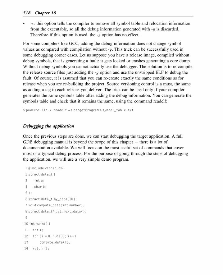
the application, we will use a very simple demo program.

1 #include,stdio.h.

2 struct data_t {

3 int a;

4 char b;

5 };

6 struct data_t my_data[10];

7 void compute_data(int number);

8 struct data_t* get_next_data();

9

10 int main() {

11 int i;

12 for (i 5 0; i,100; i11)

13 compute_data(i);

14 return 1;

518 Chapter 16

15 }

16 void compute_data(int number) {

17 struct data_t *p_data 5 get_next_data();

18 p_data-.a 5 number;

19 p_data-.b 5 number % 256;

20 }

21 struct data_t* get_next_data() {

22 static int cnt 5 0;

23 if (cnt,10)

24 return &my_data[cnt11];

25 return NULL;

26 }

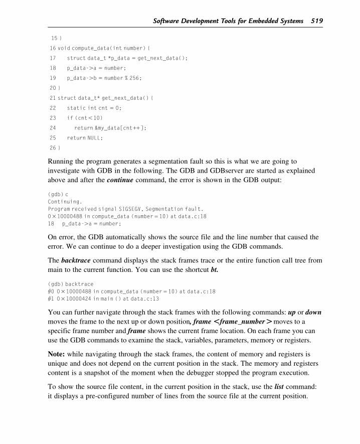
Running the program generates a segmentation fault so this is what we are going to

investigate with GDB in the following. The GDB and GDBserver are started as explained

above and after the continue command, the error is shown in the GDB output:

(gdb) cContinuing.Program received signal SIGSEGV, Segmentation fault.0310000488 in compute_data (number510) at data.c:1818 p_data-.a 5 number;

On error, the GDB automatically shows the source file and the line number that caused the

error. We can continue to do a deeper investigation using the GDB commands.

The backtrace command displays the stack frames trace or the entire function call tree from

main to the current function. You can use the shortcut bt.

(gdb) backtrace#0 0310000488 in compute_data (number510) at data.c:18#1 0310000424 in main () at data.c:13

You can further navigate through the stack frames with the following commands: up or down

moves the frame to the next up or down position, frame ,frame_number.moves to a

specific frame number and frame shows the current frame location. On each frame you can

use the GDB commands to examine the stack, variables, parameters, memory or registers.

Note: while navigating through the stack frames, the content of memory and registers is

unique and does not depend on the current position in the stack. The memory and registers

content is a snapshot of the moment when the debugger stopped the program execution.

To show the source file content, in the current position in the stack, use the list command:

it displays a pre-configured number of lines from the source file at the current position.


Examining data

Examining data (variables, memory and registers) is essential in the debugging and

investigation process and GDB offers a very good set of commands with many

configuration options.

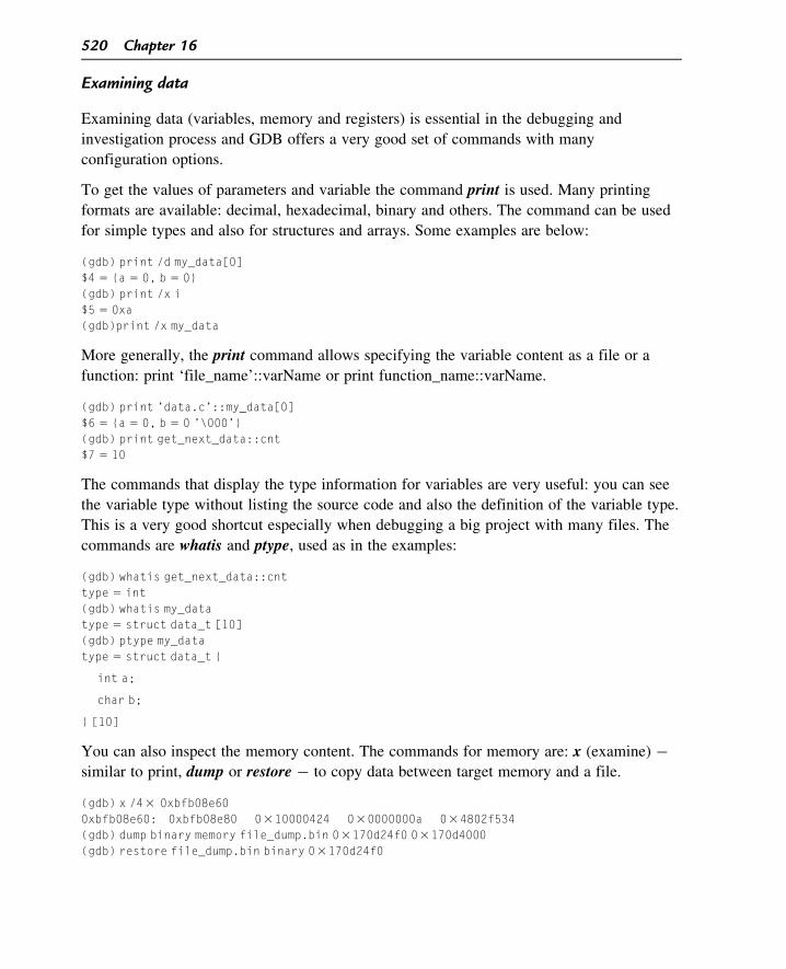
To get the values of parameters and variable the command print is used. Many printing

formats are available: decimal, hexadecimal, binary and others. The command can be used

for simple types and also for structures and arrays. Some examples are below:

(gdb) print /d my_data[0]$4 5 {a 5 0, b 5 0}(gdb) print /x i$5 5 0xa(gdb)print /x my_data

More generally, the print command allows specifying the variable content as a file or a

function: print ‘file_name’::varName or print function_name::varName.

(gdb) print ’data.c’::my_data[0]$6 5 {a 5 0, b 5 0 ’\000’}(gdb) print get_next_data::cnt$7 5 10

The commands that display the type information for variables are very useful: you can see

the variable type without listing the source code and also the definition of the variable type.

This is a very good shortcut especially when debugging a big project with many files. The

commands are whatis and ptype, used as in the examples:

(gdb) whatis get_next_data::cnttype 5 int(gdb) whatis my_datatype 5 struct data_t [10](gdb) ptype my_datatype 5 struct data_t {

int a;

char b;

} [10]

You can also inspect the memory content. The commands for memory are: x (examine) �similar to print, dump or restore � to copy data between target memory and a file.

(gdb) x /43 0xbfb08e600xbfb08e60: 0xbfb08e80 0310000424 030000000a 034802f534(gdb) dump binary memory file_dump.bin 03170d24f0 03170d4000(gdb) restore file_dump.bin binary 03170d24f0

520 Chapter 16

For advanced investigation, the low level details can be examined:

• the registers can be read with the command info registers [specific register]

• the content of the stack: read the value of the stack register and then read the memory

from that address

• disassembly: for low level debug use the disassembly to see the disassembled machine

instructions.

Using breakpoints

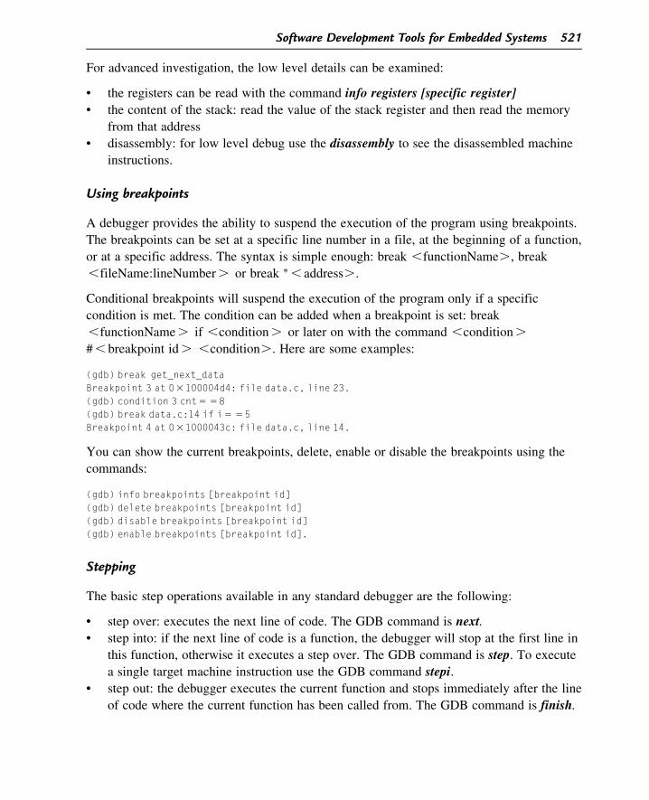
A debugger provides the ability to suspend the execution of the program using breakpoints.

The breakpoints can be set at a specific line number in a file, at the beginning of a function,

or at a specific address. The syntax is simple enough: break ,functionName., break

,fileName:lineNumber. or break � , address..

Conditional breakpoints will suspend the execution of the program only if a specific

condition is met. The condition can be added when a breakpoint is set: break

,functionName. if ,condition. or later on with the command ,condition.

#, breakpoint id. ,condition.. Here are some examples:

(gdb) break get_next_dataBreakpoint 3 at 03100004d4: file data.c, line 23.(gdb) condition 3 cnt5 58(gdb) break data.c:14 if i5 55Breakpoint 4 at 031000043c: file data.c, line 14.

You can show the current breakpoints, delete, enable or disable the breakpoints using the

commands:

(gdb) info breakpoints [breakpoint id](gdb) delete breakpoints [breakpoint id](gdb) disable breakpoints [breakpoint id](gdb) enable breakpoints [breakpoint id].

Stepping

The basic step operations available in any standard debugger are the following:

• step over: executes the next line of code. The GDB command is next.

• step into: if the next line of code is a function, the debugger will stop at the first line in

this function, otherwise it executes a step over. The GDB command is step. To execute

a single target machine instruction use the GDB command stepi.

• step out: the debugger executes the current function and stops immediately after the line

of code where the current function has been called from. The GDB command is finish.


Changing the program

While debugging a program, there are many situations when you observe how to fix the

issue, or you just want to modify the program execution. GDB provides the possibility

to modify on the fly variables, memory, registers, to call functions, return from

functions or to modify the program counter while the program is debugged. This may

save some time as compared with the standard solution: modify the code, compile it,

run the program on the target, reproduce the same error conditions and test the new

program’s changes.

Changing the program execution should be done with caution, especially when you directly

modify the registers, including the program counter, as it may cause fatal errors in the

execution.

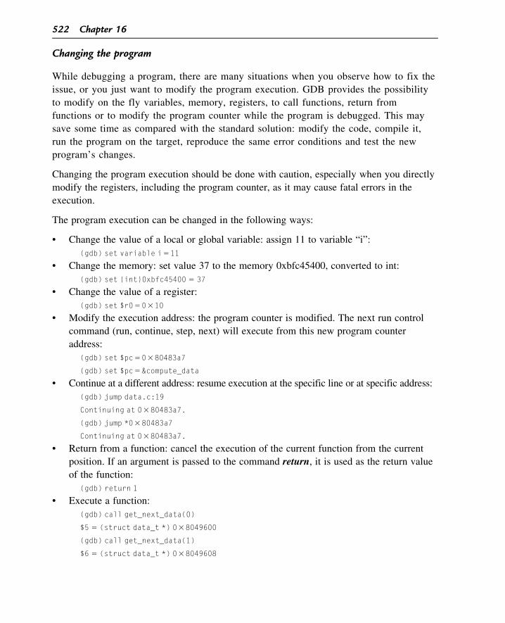
The program execution can be changed in the following ways:

• Change the value of a local or global variable: assign 11 to variable “i”:

(gdb) set variable i511

• Change the memory: set value 37 to the memory 0xbfc45400, converted to int:

(gdb) set {int}0xbfc45400 5 37

• Change the value of a register:

(gdb) set $r050310

• Modify the execution address: the program counter is modified. The next run control

command (run, continue, step, next) will execute from this new program counter

address:

(gdb) set $pc50380483a7

(gdb) set $pc5&compute_data

• Continue at a different address: resume execution at the specific line or at specific address:

(gdb) jump data.c:19

Continuing at 0380483a7.

(gdb) jump *0380483a7

Continuing at 0380483a7.

• Return from a function: cancel the execution of the current function from the current

position. If an argument is passed to the command return, it is used as the return value

of the function:

(gdb) return 1

• Execute a function:

(gdb) call get_next_data(0)

$5 5 (struct data_t *) 038049600

(gdb) call get_next_data(1)

$6 5 (struct data_t *) 038049608

522 Chapter 16

Analyzing core dumps

What is a core dump? A core dump is a binary file generated by the operating system (e.g.,

Linux) consisting of the complete status of the application (memory, registers, stack, signals

received) when the program terminates abnormally.

How are core dumps enabled? The Linux shell command “ulimit” is used to enable the core

dumps if the command is run on the console where the application will be started from.

$ ulimit -c unlimited

How are core dumps analyzed? GDB can analyze a core dump using the command:

$gdb,executable.,core dump.

Then you can use all the GDB commands except run control commands (run, continue,

stepping, call, return).

Debug agent design

We learned in the previous section how to use a standard debugger to debug and

investigate embedded applications. While widely used, a standard debugger does not

cover all the debugging scenarios. The GDB-GDBserver is an excellent debugger, but

how about the case where GDB cannot run on the target? This is quite usual, as generally

the embedded targets have special requirements and resources may be limited. Here are

some examples: the target does not run the Linux operating system, it does not have a

serial or Ethernet interface or some resource limitation does not allow porting the debug

agent. This is true not only for GDB, but for all the debuggers that use a debug agent

running on the target.

Bearing in mind these constraints, it is clear that each specific debugging scenario or corner

case may need special debugging tools and each programmer can use them to improve and

optimize at least some parts of the debugging process. For this purpose we will go through the

process of defining a debug agent framework � a generic description of how to start designing

a debug agent that fits into our special target requirements.

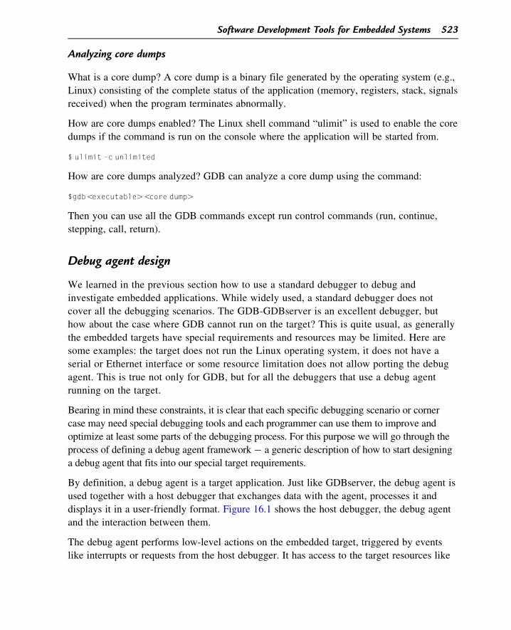
By definition, a debug agent is a target application. Just like GDBserver, the debug agent is

used together with a host debugger that exchanges data with the agent, processes it and

displays it in a user-friendly format. Figure 16.1 shows the host debugger, the debug agent

and the interaction between them.

The debug agent performs low-level actions on the embedded target, triggered by events

like interrupts or requests from the host debugger. It has access to the target resources like


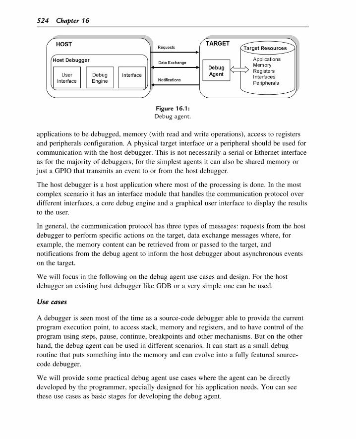
applications to be debugged, memory (with read and write operations), access to registers

and peripherals configuration. A physical target interface or a peripheral should be used for

communication with the host debugger. This is not necessarily a serial or Ethernet interface

as for the majority of debuggers; for the simplest agents it can also be shared memory or

just a GPIO that transmits an event to or from the host debugger.

The host debugger is a host application where most of the processing is done. In the most

complex scenario it has an interface module that handles the communication protocol over

different interfaces, a core debug engine and a graphical user interface to display the results

to the user.

In general, the communication protocol has three types of messages: requests from the host

debugger to perform specific actions on the target, data exchange messages where, for

example, the memory content can be retrieved from or passed to the target, and

notifications from the debug agent to inform the host debugger about asynchronous events

on the target.

We will focus in the following on the debug agent use cases and design. For the host

debugger an existing host debugger like GDB or a very simple one can be used.

Use cases

A debugger is seen most of the time as a source-code debugger able to provide the current

program execution point, to access stack, memory and registers, and to have control of the

program using steps, pause, continue, breakpoints and other mechanisms. But on the other

hand, the debug agent can be used in different scenarios. It can start as a small debug

routine that puts something into the memory and can evolve into a fully featured source-

code debugger.

We will provide some practical debug agent use cases where the agent can be directly

developed by the programmer, specially designed for his application needs. You can see

these use cases as basic stages for developing the debug agent.

Figure 16.1:Debug agent.

524 Chapter 16

Simple debug agent

In a very simple scenario, a basic debug agent runs on the target and there is no host

debugger and no communication protocol between host and target. The debug agent is

triggered on a debug event, the debug agent code is executed and it performs simple actions

such as:

• Save the debugged application context. The current state of the application is saved so

that the application execution can be resumed from exactly the same conditions, at a

later time. Typically special registers like general-purpose registers, program counter,

stack register, and link register are saved. It is mandatory to save the registers that will

be modified by the debug agent during this procedure.

• Dump the application context. The context means a set of information, depending on the

details of the processor and application design, that is relevant for the person who

interprets this information. This includes registers, stack, peripheral or interface status,

memory zone, and other application-specific data. The data can be stored in memory or

in a file if a file system is available; data can be retrieved and interpreted at a later time.

• Trigger an external event. For a low-level embedded application some information

cannot be simply saved into memory. Logical signals between different integrated

circuits on the embedded system (microcontrollers, FPGA, ASIC) or target signal

outputs (e.g., GPIO) can be read using external devices triggered by the external event

(e.g., GPIO) generated in the debug agent routine. For example an oscilloscope or a

logical analyzer device can be used to capture signals once it is triggered by the GPIO

signal from the debug agent. After triggering the external event, the debug agent can

then wait for a specific period of time, as long as the capture needs, before switching

back to the application context.

• Restore the application context. The saved application context is restored and the

application is resumed from the same conditions.

The debug event � the trigger that invokes the context switch to the debug agent code � is

an interrupt, typically a debug interrupt. Depending on the target’s processor, the interrupts

can be configured to generate debug interrupts on different exceptions. The debug event can

be also an external interrupt, triggered by an external signal assertion.

The user can also manually trigger the debug event, for example by pressing a button on

the target, or asserting an external signal, which of course generates an external interrupt.

This can be seen as a debugger “pause” command, where the application context is dumped

and the oscilloscope capture is triggered.

This is a very simple debug agent example which you may think, to some extent, can be

integrated into the application code, for example into the debug interrupt handler of the

application. While this is possible, it is not recommended. An efficient debug should be


done without modifying the application code for debug purposes as this may affect the

application functionality. Having the debug agent in a separate application allows updating

and improvement of the agent code at any time with no constraints for the application. The

debug agent can even be developed by a different team and can be further improved into a

more versatile debugger.

Simple communication protocol

For the simple scenario described above we can add a better way to retrieve the debug

information and to control the debug agent running on the target.

In the simplest scenario, one can start with a minimal host debugger and a communication

protocol that supports very basic commands. The host debugger can be implemented from

scratch, based on a very simple communication protocol. For example a request-response

based protocol will allow exchange information like:

• Control commands: the host debugger can send requests to the agent code to

• pause the application: the agent is triggered by receiving this request and makes the

context switch from the application code to the agent; the agent then waits for more

requests from the host debugger;

• continue the application: the debug agent switches back to the application context.

• Data exchange commands:

• retrieve the application context (registers, stack, application specific data);

• read and write memory.

The debug agent also needs to implement the communication protocol. On the target, a

physical interface should be reserved for communication with the host, for example serial,

Ethernet, USB or other, and it should be controlled by the debug agent. The debug agent

implements the interrupt handler on the receive side of the interface � and this interrupt is

used as a debug event trigger.

This solution is very basic in terms of debug capabilities, but has an advantage in

development time. The development time to update the simple scenario to this use case

with a basic communication protocol is short while the benefits of adding basic control of

the debug agent and data exchange capabilities are a significant improvement in the

debugging process.

Using GDB

For this use case, a full source-code debugger is needed and this requires a featured host

debugger application � which is a complex task if you want to develop it from scratch. But

instead of developing a host debugger, sometimes it is worth implementing a standard

526 Chapter 16

communication protocol in the debug agent and using the corresponding standard debugger

on the host.

The most common example is GDB: in the gdb-gdbserver mode, the host debugger is the

GDB, the debug agent is the GDBserver and the communication protocol is GDB remote

protocol, TCP or serial-based. For our case we will use the GDB and GDB remote protocol.

The debug agent will also implement the GDB remote protocol and in this way, at the

interface with the host, it is seen as a GDBserver.

If we look at the implementation requirements for the debug agent, this use case is very

similar to the previous one. Of course, developing the full set of features of the

communication protocol along with the required low-level implementation is not a small

task, but the advantages of having the fully featured GDB debugger make it worthwhile.

Multicore

This is a more complex scenario and it is provided as an example of how to use the

previously described scenarios in order to provide an efficient debugging solution.

For this scenario a multicore processor is used with Linux running on the first core while

on other cores, named secondary cores, real-time bare-board applications (with no operating

system) are running. The goal is to provide a debugging solution for the applications

running on the secondary cores.

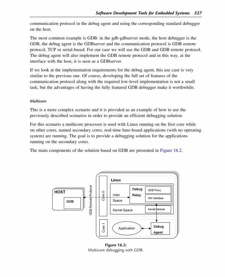
The main components of the solution based on GDB are presented in Figure 16.2.

Figure 16.2:Multicore debugging with GDB.


On the target, a debug agent is running on each secondary core. The agent can be a

symmetric multiprocessing (SMP) application � a single ELF running for all secondary cores

or, depending on the details of each target, it can be a separate ELF application for each core.

On Linux running on the first core, the debug relay is a Linux user-space application that

acts as a relay between the GDB host application and the debug agents running on the

secondary cores. The communication between the debug relay and the GDB on the host is

GDB remote protocol, TCP-based. Each debug agent is handled on a separate TCP port.

Internally, the debug relay can be based on a GDB proxy � an open-source GDB proxy

that allows target-specific interfaces to be added, with proprietary implementation. The

GDB proxy implements the communication with the host GDB (GDB remote protocol) and

therefore, for our scenario, only the target-specific interface should be implemented from

zero. In Figure 16.2, this is represented by the HW Interface module.

The communication between the debug relay and the debug agent is based on the inter-core

communication mechanisms available for the target processor. For example a shared

memory for data exchange plus an inter-core signaling mechanism (e.g., mailbox or

doorbell) can be used.

The host debugger is GDB and if required it can be used as a graphical user interface, GDB

compatible. From the host, the debug relay and the debug agents are seen as multiple

GDBserver applications running on separate TCP ports, one for each secondary core.

There are some advantages for this scenario, as compared with the previous use cases:

• The solution provides a full-featured GDB debugger, but the development time is

reduced by using the GDB on the host and the GDB proxy on the target. Only the

target-specific modules are implemented: the debug agent and the communication

protocol with the debug relay.

• In the previous use cases, a hardware resource is reserved for the debug agent to be

used for communication with the host debugger. In the current solution there is no such

restriction as the Ethernet port can be shared with all other Linux applications.

Debug agent overview

As you learned in the previous sections where and how to use the debug agent, in the

following we will go deeper into the implementation details of the debug agent and point

out the key elements of the design.

The debug agent is a bare-board application running directly on the target with no

operating system (OS). It has no knowledge about Linux or any operating system.

The application to be debugged is also seen as a bare-board application, with no OS awareness.

528 Chapter 16

The application itself can be an operating system, for example Linux, and the debug agent is

able to do a Linux kernel debug, handling Linux as a simple bare-board application.

We will assume in the following that the host debugger is GDB and it communicates with the

agent using GDB remote protocol, directly or through a GDB proxy. This allows a complete

description of the agent design, based on the features provided by GDB. On the other hand,

the debug agent design principles are the same, independent of the host debugger’s type.

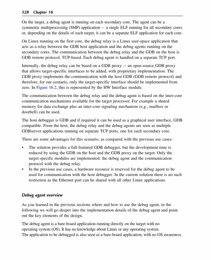
Figure 16.3 presents how the debug agent interacts with the debugged application on the target.

The debug agent is a separate ELF application with its own code, data, stack and heap

segments. The application memory space does not overlap with the debug agent memory

space. Moreover, as a very valuable feature, the debug agent code should be made position-

independent executable; meaning that the memory address from where the agent’s code is

executed can be changed. This way, the user can configure the run address of the debug agent

at the desired location.

Depending on each specific debug scenario, the debug agent can load and start the

application or just attach to an already running instance of the application. In any case, the

debug agent does not interpret the application ELF; this is done by the host debugger.

Application start can be seen as a context switch from debug agent to application, with a

clean application context.

The context switch is triggered by a debug event that can be:

• a debug interrupt caused by an exception in the application, in which case the context is

switched from the application to the agent, or

Figure 16.3:Debug agent overview.


• a request from the host debugger that internally generates an interrupt (e.g., a receive

data ready interrupt) that, depending on the request, triggers the context switch to the

application (e.g., “continue” command) or to the debug agent (e.g., “pause” command).

The debug agent should be able to access the application’s address space. It needs read and

write access to data, stack and heap so that the host debugger can read and write application

variables, read the stack frames and read and write to memory.

These key points will be detailed below.

Starting the application

One possible use case is where the application is loaded and started by the use of the

debugger. This way, the application execution can be debugged from the first instruction.

Before starting the application, there are some preconditions that have to be met:

• the application is compiled with debug symbols and the ELF file is available in the host

debugger;

• the debug agent is running on the target and the connection with the host debugger is

up and running;

• the host debugger should support the download capability; for GDB, this is

implemented in the command “load”.

Through this process, some steps are done by the host debugger and some by the debug

agent. To understand the design and implementation requirements for the debug agent we

will go step by step through the application download process from the host debugger to

the agent.

On the “load” command, the following actions are performed:

• The binary image of the application is copied into the target memory. This is done by

sending a “write memory” request to the debug agent, containing the binary data and

the target memory address where data should be written.

• The program counter register (PC) is set to the application entry point � the memory

address where the first application instruction should be executed. A “write register”

request is sent to the agent, containing the register number and the value to be set.

• The application is now ready to start. It can be started with a different command,

“continue”.

As you can see, the debug agent performs simple actions like writing memory and

assigning a value to a register. The complex tasks are done in the host debugger and we can

see again the advantages of using the split solution (debugger host1 debug agent).

530 Chapter 16

The other use case is where the application has been started before the debugger connects

to it, through the debug agent. On the attach process, the host debugger triggers a debug

event to the debug agent and a context switch is started from the application to the

debug agent.

Context switch

In the process of a context switch, the execution is changed from the application ELF to the

debug agent ELF or vice versa. The context represents the current application states

necessary to be able to resume the application from the same point and same conditions at a

later time. Typically, in the context general-purpose registers, program counter, stack

register, and link register are saved. The application to be debugged has no knowledge

about the debug agent and therefore does not handle the context switch. The saving and the

restoring of the application context is done in the debug agent code and it is triggered by

debug events such as debug interrupts or interrupts triggered by requests from the host

debugger.

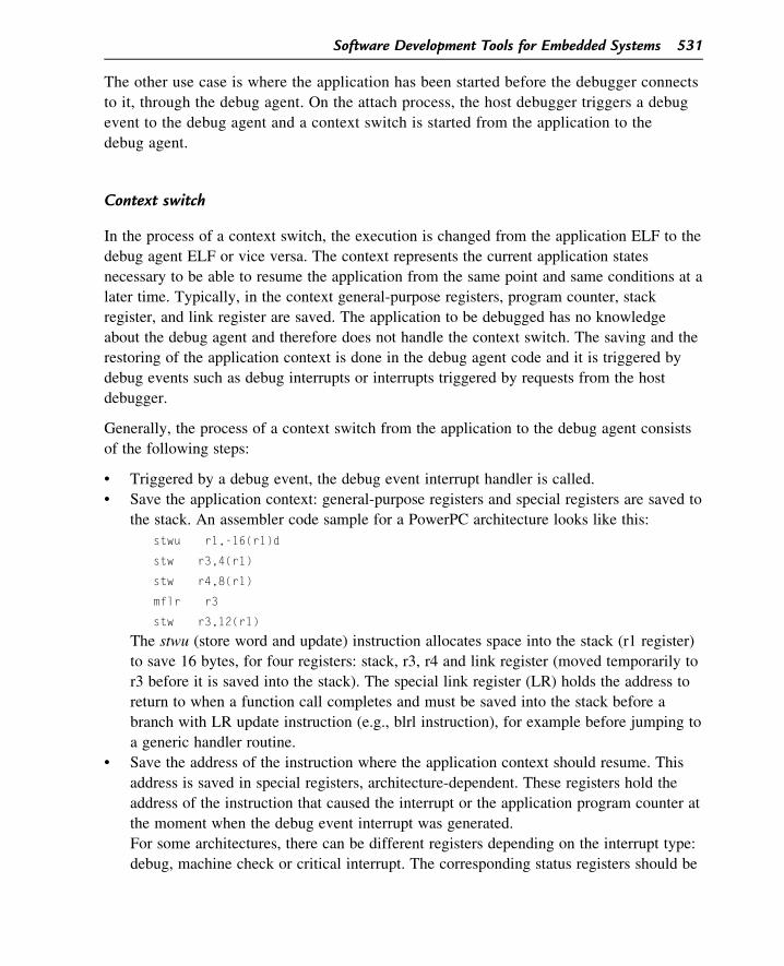
Generally, the process of a context switch from the application to the debug agent consists

of the following steps:

• Triggered by a debug event, the debug event interrupt handler is called.

• Save the application context: general-purpose registers and special registers are saved to

the stack. An assembler code sample for a PowerPC architecture looks like this:

stwu r1,-16(r1)d

stw r3,4(r1)

stw r4,8(r1)

mflr r3

stw r3,12(r1)

The stwu (store word and update) instruction allocates space into the stack (r1 register)

to save 16 bytes, for four registers: stack, r3, r4 and link register (moved temporarily to

r3 before it is saved into the stack). The special link register (LR) holds the address to

return to when a function call completes and must be saved into the stack before a

branch with LR update instruction (e.g., blrl instruction), for example before jumping to

a generic handler routine.

• Save the address of the instruction where the application context should resume. This

address is saved in special registers, architecture-dependent. These registers hold the

address of the instruction that caused the interrupt or the application program counter at

the moment when the debug event interrupt was generated.

For some architectures, there can be different registers depending on the interrupt type:

debug, machine check or critical interrupt. The corresponding status registers should be


read to find out what type of interrupt has been called and therefore what register

registers should be saved.

• Initialize the stack for the debug agent. The application and the debug agent have

separate stacks. In the interrupt handler, the stack register is set to the application stack.

For further high-level processing, the debug agent should use its own stack, while the

application stack along with the application saved context should be used for the

application debugging. The debug agent stack can be initialized as in the example:

lis r1, _stack_addr@ha

addi r1, r1, _stack_addr@l

If the debug agent is an SMP application running on multiple cores, separate stacks for

each core should be used and here the stack initialization should be done accordingly.

• Interrupt handling while the debug agent is running: depending on the application

functionality some interrupts should be enabled and some disabled when switching the

context to the debug agent. This behavior should be configurable in the debug agent.

• The execution is passed to the main program loop of the debug agent, a C-code high-

level handler. The application stack value should be passed as a parameter � for each

processor architecture there are specific registers for passing parameters from assembler

to C code. A direct branch or an LR instruction can be used (bl, blrl) or a return from

interrupt call (rfi) after the corresponding registers have been set (LR or interrupt save/

restore registers).

After the high-level handler has been called, the context switch is completed. Now the

debug agent is running, it communicates with the host debugger and it is able to do the

basic debug functions:

• Read and write registers: on the host debugger request, the debug agent is able to

access the registers. The real registers are not actually accessed but the temporary

location where the registers values have been retrieved after the application context

save. On writing a register, the new value will of course apply after the application

context is restored.

• Read and write memory and stack: unlike the registers, the memory, including stack, is

directly accessed for read and write operations. The debug agent can have access to the

entire memory space. The stack register value is retrieved from the saved application

context (e.g., r1 register).

• Breakpoints: in the debug agent implementation, setting software breakpoints means

writing the application’s code memory zone. Based on the symbolic information in the

application ELF, the host debugger finds the address corresponding to the breakpoint

location at a specific symbol or at a specific line number. When a breakpoint is set, the

host debugger sends this address to the target. The debug agent just replaces the

assembler instruction at this address with a special instruction that generates a debug

exception.

532 Chapter 16

• Run control: stepping, continue. Stepping can be implemented as a breakpoint to the

next instruction and a continue command. The continue command triggers the context

switch from the debug agent to the application, where the application context

is restored.

On context restore, the debug agent performs steps similar to the context save. The

application registers are restored from the temporary location where they may have been

modified on user request. The PC is not directly set, but the save/restore registers are

restored. The context restore is completed with a return from interrupt call.

Position-independent executables

Position-independent code (PIC) and position-independent executables (PIE) allow an

executable to run independently of the position in the memory where it resides. The same

code, within the same ELF file, can be copied to any memory address and can run with no

changes.

This is very important, as we have seen that the application to be debugged and the debug

agent have independent memory address spaces that should not overlap. To give an

example, let us assume that the debug agent is compiled to run from a hard-coded memory

address (position dependent executable). If the application’s memory requirements change

and the address space overlaps with the debug agent’s memory space, then the debug

agent would need to be rebuilt to adjust the run address to the new memory addresses.

This is not practical and the programmer that is doing debug of the application would

prefer not to rebuild the debug agent every time the memory spaces change. In addition,

if the debug agent is provided without source code, it is a problem having a hard-coded

run address.

Let us see how the position-independent executable is implemented for our debug agent.

First, it is preferable that the compiler has support for position-independent executables.

This is not a strict requirement; the code can be specially written to be position-independent

without using absolute values for branch and for data section. While possible, this is

recommended only for a small number of code lines.

For the GCC build tool chain, a position-independent executable is enabled by adding the

options “-fPIE” for compiler and linker. With this option, the function calls and the access

to data variables are done through an indirection table, named Global Offset Table (GOT).

The GOT table stores the addresses of all functions and global variables. For a position-

independent executable, only the addresses from the GOT table have to be updated, at run-

time, corresponding to the current load address of the program while the rest of the program

remains unchanged.


Along with the build tool chain support at compile time, there are some other requirements

for run-time, to be executed from the debug agent code: compute the current load address

of the program and update the GOT table accordingly to this value.

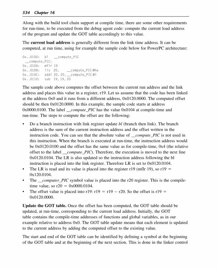
The current load address is generally different from the link time address. It can be

computed, at run time, using for example the sample code below for PowerPC architecture:

0x..0100: bl __compute_PIC__compute_PIC:

0x..0104: mflr 190x..0108: lis 20, __compute_PIC @ha0x..010C: addi 20, 20, __compute_PIC @l0x..0110: sub 19, 19, 20

The sample code above computes the offset between the current run address and the link

address and places this value in a register, r19. Let us assume that the code has been linked

at the address 0x0 and it runs from a different address, 0x0120.0000. The computed offset

should be then 0x0120.0000. In this example, the sample code starts at address

0x0000.0100. The label __compute_PIC has the value 0x0104 at compile-time and

run-time. The steps to compute the offset are the following:

• Do a branch instruction with link register update bl (branch then link). The branch

address is the sum of the current instruction address and the offset written in the

instruction code. You can see that the absolute value of __compute_PIC is not used in

this instruction. When the branch is executed at run-time, the instruction address would

be 0x0120.0100 and the offset has the same value as for compile-time, 0x4 (the relative

offset to the label __compute_PIC). Therefore, the execution is moved to the next line

0x0120.0104. The LR is also updated so the instruction address following the bl

instruction is placed into the link register. Therefore LR is set to 0x0120.0104.

• The LR is read and its value is placed into the register r19 (mflr 19), so r19 5

0x120.0104.

• The __computer_PIC symbol value is placed into the r20 register. This is the compile-

time value, so r20 5 0x0000.0104.

• The offset value is placed into r19: r19 5 r19 � r20. So the offset is r19 5

0x0120.0000.

Update the GOT table. Once the offset has been computed, the GOT table should be

updated, at run-time, corresponding to the current load address. Initially, the GOT

table contains the compile-time addresses of functions and global variables, as in our

example relative to address 0x0. The GOT table update means that each element is updated

to the current address by adding the computed offset to the existing value.

The start and end of the GOT table can be identified by defining a symbol at the beginning

of the GOT table and at the beginning of the next section. This is done in the linker control

534 Chapter 16

file (LCF) as in the following example, where __got1_start and __dynamic_start identify

the GOT table beginning and end:

got1 : {

__got1_start 5 .;

*(.got1)

}

.got2 : { *(.got2) }

.dynamic : {

__dynamic_start5 .;

*(.dynamic) }

The sample code below shows how the addresses are updated in the GOT table. It is

assumed that the offset has been previously computed and placed into the r19 register.

register int offset 5 0;asm (“mr %0, 19” : “5r” (offset));

volatile unsigned int* got_start 5

(unsigned int*)((unsigned int)&__got1_start1 offset);

unsigned int count 5

((unsigned int)&__dynamic_start �(unsigned int)&__got1_start)/sizeof(unsigned int);

for (int i 5 0; i,count;11i)

got_start[i] 1 5 offset;

There is a small performance penalty when enabling position-independent code, because of

the functions and data variable access through the GOT table. So it is not always a good

idea to have this feature, especially for real-time applications. For the debug agent this is

not an issue.

Debug event from the application

The debug event from the application is the debug interrupt, triggered whenever an

exception occurs (breakpoints or application errors). In the simplest scenario, when the

exception occurs, the debug interrupt of the debug agent should be called and, as we

learned in the previous sections, the context is switched from the application to the

debug agent.

The principle is simple, but putting it into practice can be sometimes a challenge. The

design of the debugged application should not consider doing anything special for

integration with a debug agent. Therefore the application will do the normal initialization of

the interrupt vector table, and the offset for debug interrupt. If a debug exception occurs


when running the application without the debug agent, then the debug interrupt handler of

the application is called � the handler is therefore in the application code.

When debugging the application with our debug agent, then something should be changed

so that, on a debug event, the debug interrupt handler of the agent will be called. The

application should be able to use all other interrupts while, for the debug interrupt only, the

agent’s handler will be called. If it is possible to specify a configurable interrupt vector

address only for the debug interrupt, then this can be a very simple solution: when starting,

the debug agent would set the debug interrupt address to point to its handler. Unfortunately,

this is not possible on many processors: you can only specify a base address for the

interrupt table and an offset for each interrupt type.

For these scenarios it is clear that the application debug interrupt is called and the solution

is to move the execution, from the application interrupt handler, through a branch

instruction, to the debug agent interrupt handler. Of course, this should not add

requirements to the application code to hard-code a branch in its debug interrupt handler.

Moreover, the load address of the debug agent is not known at compile time. The solution

is that the debug agent would overwrite the application’s debug interrupt handler, so the

desired branch is executed, as described in Figure 16.4.

A sample code used to overwrite the application’s debug interrupt is presented below, for

the PowerPC processor:

1 app_handler_start:2 stwu 1, -16(1)3 stw 3, 4(1)4 stw 4, 8(1)5 mflr 3

Figure 16.4:Debug event from the application.

536 Chapter 16

6 stw 3, 12(1)7 lis 4, debug_agent_handler@h8 ori 4, 4, debug_agent_handler@l9 mtlr 410 blrl11 app_handler_end:12 nop

First, the necessary space is allocated in the stack for saving all the registers modified in

this routine: stack register, link register, r3 and r4 registers. Then a branch is executed to an

absolute address, through LR, to the debug agent interrupt handler address. After the

branch, in the debug_agent_handler these saved registers must be used in the context save

procedure.

The debug agent will copy the above code to the address of the debug interrupt vector of

the application. Actually the memory is overwritten with the instruction code resulting after

the compilation of these lines. This can be done in the agent code, as in the example below:

void* app_handler_start_addr 5 &&app_handler_start;void* app_handler_stop_addr 5 &&app_handler_stop;int size 5 app_handler_start_addr - app_handler_start_end;

memcpy((void*)app_debug_int_addr, app_handler_start_addr, size);

The variable app_debug_int_addr is the debug interrupt address of the application.

Let us consider also the case described above where the debug agent is a position-independent

executable. At the debug agent compile-time, the code for the application debug handler is

compiled and transformed into instruction code. At this time, the function debug_agent_handler

has the predefined offset before knowing the application load address. Then when the

instruction code is written in the application memory, the instructions at lines 7 and 8 will still

contain the compile-time value of the function, so this is not the expected, run-time value.

The correct value of the agent debug handler can be computed based on the following:

• In the agent code, at run time, the address of the debug handler function has the run-

time value as the GOT table has been updated with the current load address.

• The assembler instructions that set the address of the debug handler in lines 7 and 8

need to be updated to reflect the run-time address of the handler. Looking at the

instruction definition, the address is set in the least-significant 16 bits of the instruction.

Below is the code that updates the address of the debug handler to the correct run time

value.

unsigned int relocated_addr 5 (unsigned int)& debug_agent_handler;unsigned int *instr_addr 5 ((unsigned int *) app_debug_int_addr1 5);*instr_addr 5 ((*instr_addr) & 0xFFFF0000) j


((relocated_addr.. 16) & 0xFFFF);

11instr_addr;*instr_addr 5 ((*instr_addr) & 0xFFFF0000) j

((relocated_addr) & 0xFFFF);

There is one more thing to clarify: how to find the address of the debug interrupt vector of

the application (app_debug_int_addr). There are several ways to obtain this address,

depending on each use case scenario:

• In the case where the debug agent attaches to an already running instance of the

application, the interrupt vector is assumed to be set in the application. The debug

interrupt address can be computed reading some special registers. For example, for

PowerPC architecture the address is the sum of values in the registers IVPR (base

interrupt address) and IVOR15 (debug interrupt offset).

• The above case cannot be use for early debug of the application before the application

sets the interrupt vector. For this case, the debug agent can set the interrupt vector

pointing to its address space. The debug interrupt address would in this case be chosen

by the debug agent.

• A complete solution is to configure the debug agent with the application’s debug

interrupt address. This case can be implemented in different ways, for example:

• Pass the address as start parameter by setting this value into a hardcoded register.

• Set the parameter from the host debugger. In the case of a GDB host debugger, the

monitor command allows the sending of a special request to the debug agent. The

address can be transmitted for example using the command monitor debug_addr

,address..

Multicore

The debug agent can run on single-core or multicore processors. The design principle is the

same, but for multi-core there are several things we have to consider. The debug agent can

be an SMP executable, a single ELF file, running for all cores, or it can be an individual

ELF running on each core. The preferred approach is to have a single SMP executable for

all cores, having more flexibility in the debug agent usage: the ELF file is loaded only one

time, the code section is reused for all cores, the reserved memory space is compact and the

development and build process is simpler. Even in an SMP application, the cores can

independently execute the code: some cores can be paused while others are running.

Context switch must be correctly handled for a multicore processor since on each core the

debug agent will use its own stack and the application has a different context for each core

(stack and registers).

538 Chapter 16

One of the use cases presented in this chapter is the multicore scenario that combines

multicore capabilities with the flexibility of having an operating system on one core: the

case where Linux runs on the first core while the secondary cores run real-time bare-board

applications (with no operating system). For this case, the debug agent should implement

communication with the debug relay running on Linux, based on the following:

• Data exchange between the debug agent and debug relay on Linux is done through a

shared memory zone. The memory can be accessed with read and write operations by

both agent and relay. A simple approach is to use a circular memory buffer, with read

and write pointers.

• The access to the shared memory zone from different cores should be protected by a

spin lock mechanism. For example, a spin lock test-and-set mechanism should be used

to protect common accesses. The implementation depends on the processor’s

synchronization mechanisms (e.g., memory barrier).

• An inter-core signaling mechanism should be implemented to notify the other core that

data is available on the shared memory. This should be an interrupt-based mechanism.

Polling would not be a valid solution since the mechanism should be able to trigger, for

example, the context switch from the application to the debug agent. And so, while

polling can be implemented in the debug agent code, it is not a solution when the

application context is running.

• A processor may provide more than one inter-core signaling mechanism. Some

mechanisms use a special interrupt to handle an event from the other core. For example,

a doorbell inter-core interrupt has a special doorbell interrupt handler. If the debug agent

used this interrupt, the doorbell interrupt could no longer be used in the application,

which adds some resource limitations when debugging with our debug agent. If it is

possible, an inter-core interrupt based on the debug interrupt would be a better choice.

Starting the debug agent

We have seen above how to start the application and debugging it using the debug agent.

We will describe below how to start the debug agent.

Some targets may have a boot loader or a monitor program that is able to load other

executables using a command-line interface. An example of such a boot loader is u-boot. In

this case, the debug agent loading is handled by the boot loader.

If the target does not have a boot loader program, the debug agent binary should be copied

into a non-volatile memory; for example, NOR, NAND or SPI flash memory. When

booting from the flash memory, the program has to do some supplementary steps as

compared to booting from RAM memory: at the reset address, set a jump to the program


code in flash, do the relocation of the binary from flash to RAM and run from RAM. This

is valid for any executable booting from flash.

For the multicore scenario with Linux running on the first core, we can use a different

approach to load and start the debug agent. The process is performed completely from

Linux with no other requirements for the debug agent.

The loading of the debug agent program consists of copying the agent binary into the

memory, at the desired memory address. A Linux application should be able to access the

physical memory location where the debug agent program should be loaded. The binary

will be directly copied into the memory. If the debug agent is a position-independent

executable, then it can be copied and run from any memory location. The conversion from

ELF file to binary can be done using the build tool chain utilities, or the Linux application

can handle this conversion.

The starting of the debug agent is a little more complicated than loading. The Linux

running on the first core cannot access the other cores’ registers and it can only execute

instructions on the first core. The execution start can be done similarly to how Linux starts

the secondary cores in an SMP scenario. The u-boot boot loader provisions the boot code

for the secondary cores so that the secondary cores enter, immediately after they have been

enabled, into a spin loop. Each secondary core stays in the spin loop until a specific

memory address is written with the address in which to jump out of the loop. Therefore, in

order to start the debug agent on a secondary core, the Linux loader application writes into

the spin loop jump address the value of the agent’s entry point. The secondary core will

then exit the spin loop and start executing the debug agent’s code.

Another possibility to load and start the debug agent is to use the JTAG probe. We will

describe how to use the JTAG in the next section.

Debugging using JTAG

The name JTAG comes from Joint Test Action Group and was standardized later as the

IEEE standard 1149.1 � Standard Test Access Port and Boundary-Scan Architecture. It was

initially designed and used for testing integrated circuits using a boundary scan. Currently,

the JTAG usability extends to a wider scope, including circuits and boundary scan testing,

debugging embedded systems including processors and FPGA circuits, data transfer into

internal flash memory of circuits, flash programming, trace and analysis.

In the following we will focus on the JTAG usage for debugging embedded systems. The

host debugger software uses the JTAG probe for low-level access to the embedded system

resources such as read and write registers, read and write memory and complete run control

of the target with operations such as run, continue or stepping. Through the use of JTAG,

540 Chapter 16

the host debugger provides a featured set of debugging capabilities that allows developers

to save development time during target bring-up and debugging. The high-level debugging

capabilities such as operating system awareness (e.g., Linux kernel awareness), kernel

module drivers, Linux user-space and kernel-space debugging or hypervisor awareness are

features provided by the host debugger, while the JTAG executes only basic commands

between the host and the target.

Physically, the JTAG is an external device. It connects to the target via a special JTAG pin

header connector through a special JTAG cable. For the connection to the host USB,

Ethernet or parallel or serial ports can be used.

It is worthwhile mentioning here that along with the JTAG there are also other interfaces

available for debugging through an external probe. One example is the ARM Cortex-M

debug interface Serial Wire Debug (SWD) � a low-cost interface with only two pins and

the single-bit serial wire output (SWO). These interfaces use the ARM debug modules

Instrumentation Trace Macrocell (ITM) and Embedded Trace Macrocell (ETM). For full

instruction trace, the ETM module provides real-time trace over a 4-bit high-speed port.

Overall, this interface provides more powerful debug capabilities with the advantage of

lower pin count.

The debugging principles are the same for these debug interfaces and for generality we will

refer in the following to the JTAG.

Benefits of using JTAG

When we talk about debugging with JTAG we are referring to a complete debugging

solution including featured host debugger software along with the capabilities of controlling

the target through the JTAG.

The main advantages of debugging using JTAG are the short development time for

embedded system applications and low-level support for initial board bring-up, validation

and development.

To better understand the benefits of using JTAG, let us assume an example where the

embedded developer receives a new target and is required to do the board validation and to

develop an application on the target. How can he start developing and debugging his

application? Of course, in the end, these tasks can be done without using a debugger but at

a time cost. On the other hand, a debugger would allow a very fast development time. We

also learned that the debug agent software can be developed to run on the target, allowing

debugging of the user’s application. But how long would it take to develop the debug agent

itself? And what debugging tools can be used while developing the debug agent? For this

case, a debugging solution using the JTAG can be the key: there is no need to develop or to


use existing supplementary software (e.g., debug agent) for debugging the application. It

provides the complete set of debugging tools to start investigating the application, even for

the initial board bring-up.

In addition, debugging with JTAG provides some other capabilities through the host

debugger interface, such as the following:

• Initialization files: the debugger provides the possibility of using target initialization

files containing the initial settings of the target immediately after power-up. For

example, it can contain memory controller set-up, register set-up, RAM memory

initialization.

• The target can be completely controlled without running software on the target. The

registers and memory can be directly accessed through the special JTAG interface and

it is not required that the processor or the core actually execute instruction code. This is

important as the registers or memory can be accessed even if the core is not enabled.

• Integrated bare-board application development including target reset, initialization file

and application download into the RAM memory.

• Read and write access to the processor’s internal flash memory.

• JTAG debugging is non-intrusive in the application to be debugged.

Board bring-up using JTAG

For the initial board bring-up of an embedded system, debugging using JTAG allows a very

fast target validation and application development. The bring-up target specific settings are

typically done in the initialization file. The debugger allows the reuse of the initialization

file every time a new application is downloaded to the target. An advantage of debugging

using the JTAG for initial board bring-up is the use of the initialization file. Based on it, the

target can be controlled through the JTAG without executing code on the processor. Some

examples of target-specific initialization settings are the following:

• memory management unit (MMU) initialization;

• translation lookaside buffer (TLB) initialization � virtual to physical memory address

translations are stored in the TLBs; the TLB for DDR memory and for the other

memory-mapped peripherals should be defined here;

• local access windows set-up (LAW) (only specific to some processors);

• DDR controller set-up: timing, bus frequency configurations;

• interrupt vector initialization;

• register configuration for peripherals, like flash memory;

• target-specific register initialization;

• debug register settings, like enabling the debug interrupt, enabling the external debug

mode (for JTAG);

542 Chapter 16

• core initialization for multicore processors. By default, the secondary cores are disabled.

It is the first core that should do the initialization for the secondary core, or, in our

case, it can be done by the debugger using the initialization file.

Comparison with the debug agent

Both cases of debugging using JTAG and debugging using a debug agent running on the

target are widely used for embedded system development. Each solution has some

advantages and, based on this, each solution is more often used in certain circumstances:

• JTAG for initial board bring-up, early application debug and when the debug agent

software is not available, typically for bare board applications with no operating

system;

• debug agent for high-level debug, typically after some operating system services are

available for the debug agent. A common case is Linux user-space application debug

using GDB/GDBserver.

In the following we will present some practical use case examples of debugging with JTAG

or debug agent.

• For early Linux kernel debug, the better solution is to use JTAG debugging. In this

case, the kernel can be debugged from the first instruction, the JTAG is not intrusive in

the kernel and the kernel can be completely debugged: kernel core and all drivers. On

the other hand, the debug agent solution using KGDB is too limited: the kernel can be

debugged only after the KGDB module is loaded and only some parts of the kernel can

be debugged. This is an intrusive debugging method where executing the KGDB

module may influence the kernel functionality.

• JTAG debugging can provide powerful features like Linux kernel and user-space

awareness, allowing debugging at the same time of the Linux user-space applications

and kernel. The program execution can be debugged while moving from the user-space

application to kernel space through system calls or kernel module functions.

• The bare-board debug agents need a hardware resource (e.g., serial or Ethernet port)

reserved for communication with the host debugger. For JTAG debugging there is no

restriction as the JTAG interface is dedicated to communication with the host debugger.

For some debug agents like GDB/GDBserver, the communication channel (IP interface)

to the host debugger can be shared with the other user-space applications.

• For JTAG debugging, the registers and memory can be directly accessed and it is not

required for the processor to be enabled or to execute instruction code. This is the main

advantage over debug agents for the initial board bring-up.

• Remote access: debug agents generally have support for Ethernet communication and

can be accessed remotely. JTAG devices with remote access over Ethernet can be


expensive. For USB JTAG devices a trade-off is to use a computer near the equipment

to solve the remote access issue.

• For some scenarios, JTAG debugging is not a practical solution. Let us assume for

example we need to debug base station equipment with three or six sector

controllers, each running on separate hardware. Having three or six JTAG devices

connected to each sector controller is not a practical solution. On the other hand,

debug agent software can be embedded in the sector controller, also allowing remote

debugging.

• JTAG debugging is most likely to be used in the lab while the software is being

developed or investigated. For the final products or equipment installed in the field,

connecting the JTAG may be difficult or impossible. The JTAG pin header connector is

located on the equipment mother-board and the equipment box has to be opened in

order to connect the JTAG device. And of course you cannot have JTAG devices

connected to all the equipment in the field.

• For field equipment, debug agents, like GDB, offer reliable solutions: if remote access

is available the application can be remotely debugged and without remote access the

application’s crash dump can be analyzed offline.

• JTAG debugging can only be used if the processor has JTAG support and the JTAG pin

header is available on the hardware. For some pieces of equipment, due to constraints

of space, power consumption or electromagnetic compliance, the hardware is designed

without the JTAG pin header. In this case, development boards with JTAG pin header

should be used for the initial board bring-up and, after the software is stable,

development can be continued on the final hardware. The debugging can then be

continued based on a debug agent solution.

• Some JTAG devices, especially those with remote access (Ethernet, gigabit), can be

expensive, especially where a license is needed for debugger software. When one

chooses a debugging method it is always based on a trade-off between price and

capabilities.

GDB and JTAG

We have seen above the advantages of debugging using JTAG as well as the flexibility of

the open-source GDB debugger. For embedded system debugging, GDB is commonly used

with a debug agent, like GDBserver, running on the target. However, GDB flexibility

allows the integration of GDB and JTAG devices.

One of the commonly used cases is the early Linux kernel debug: as described above,

debugging with JTAG would allow a complete and reliable debug, while the KGDB

solution is an intrusive solution that covers only some parts of the kernel debugging.

544 Chapter 16

The solution of GDB debugging using JTAG is based on the following.

• There will be no debug agent running on the target. The target will be accessed only

through the JTAG.

• On the host, the GDB host debugger will be compiled for cross debugging of the embedded

target. Optionally, any available graphical user interfaces can be used, like for a normal

GDB debugging. No change is required in GDB for integration with the JTAG device.

• A GDB relay software program will act as a relay between the GDB host debugger and

the JTAG. The GDB relay is a host application (e.g., a Linux user-space application)

and can run on the same host as GDB or on a different host. The GDB relay

implements the GDB remote protocol at the interface with the GDB and, therefore,

from the GDB host debugger, the GDB relay is seen as a GDBserver.

• The communication with the JTAG is implemented in GDB relay software. This is

specific to each supported JTAG device. The JTAG can be accessed remotely

(Ethernet) or locally (USB).

• Internally, the GDB relay can be based on a GDB proxy � an open-source GDB proxy that

allows the addition of target-specific interfaces, with proprietary implementation. The GDB

proxy implements the communication with the host GDB (GDB remote protocol) and only

the interface for the communication with the JTAG should be implemented.

Special JTAG commands can be passed using the GDB “monitor” command. The GDB

initialization file (.gdbinit) can be used for the JTAG initialization file.

Currently, many open-source solutions are already available for the integration of GDB and

JTAG, for many processors and different JTAG devices.

Debugging tools using Eclipse and GDB

In this section we present an example of how to use free open-source software to obtain an

integrated development and debugging tool providing standard debug capabilities for Linux

user-space application debug and Linux kernel debug. We will use the following open-

source software:

• GDB/GDBserver for low-level support for debugging the applications on the embedded

target. We have seen above how to download, compile, configure and use GDB for our

target.

• KGDB � this is a kernel functionality that allows the kernel to be debugged over a

serial line or Ethernet from a remote host. The remote host uses GDB for connecting to

the running kernel on the target through the interface provided by KGDB.

• Eclipse � Eclipse is an open-source community focused on building an open

development platform for extensible frameworks, tools and run-times for debugging,


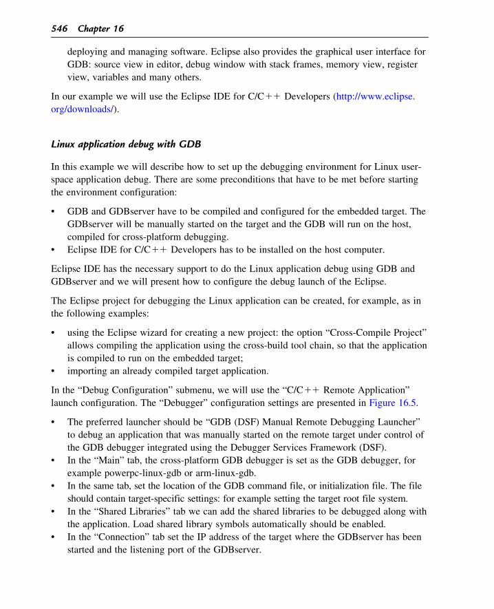
deploying and managing software. Eclipse also provides the graphical user interface for

GDB: source view in editor, debug window with stack frames, memory view, register

view, variables and many others.

In our example we will use the Eclipse IDE for C/C11 Developers (http://www.eclipse.

org/downloads/).

Linux application debug with GDB

In this example we will describe how to set up the debugging environment for Linux user-

space application debug. There are some preconditions that have to be met before starting

the environment configuration:

• GDB and GDBserver have to be compiled and configured for the embedded target. The

GDBserver will be manually started on the target and the GDB will run on the host,

compiled for cross-platform debugging.

• Eclipse IDE for C/C11 Developers has to be installed on the host computer.

Eclipse IDE has the necessary support to do the Linux application debug using GDB and

GDBserver and we will present how to configure the debug launch of the Eclipse.

The Eclipse project for debugging the Linux application can be created, for example, as in

the following examples:

• using the Eclipse wizard for creating a new project: the option “Cross-Compile Project”

allows compiling the application using the cross-build tool chain, so that the application

is compiled to run on the embedded target;

• importing an already compiled target application.

In the “Debug Configuration” submenu, we will use the “C/C11 Remote Application”

launch configuration. The “Debugger” configuration settings are presented in Figure 16.5.

• The preferred launcher should be “GDB (DSF) Manual Remote Debugging Launcher”

to debug an application that was manually started on the remote target under control of

the GDB debugger integrated using the Debugger Services Framework (DSF).

• In the “Main” tab, the cross-platform GDB debugger is set as the GDB debugger, for

example powerpc-linux-gdb or arm-linux-gdb.

• In the same tab, set the location of the GDB command file, or initialization file. The file

should contain target-specific settings: for example setting the target root file system.

• In the “Shared Libraries” tab we can add the shared libraries to be debugged along with

the application. Load shared library symbols automatically should be enabled.

• In the “Connection” tab set the IP address of the target where the GDBserver has been

started and the listening port of the GDBserver.

546 Chapter 16

http://www.eclipse.org/downloads/

http://www.eclipse.org/downloads/

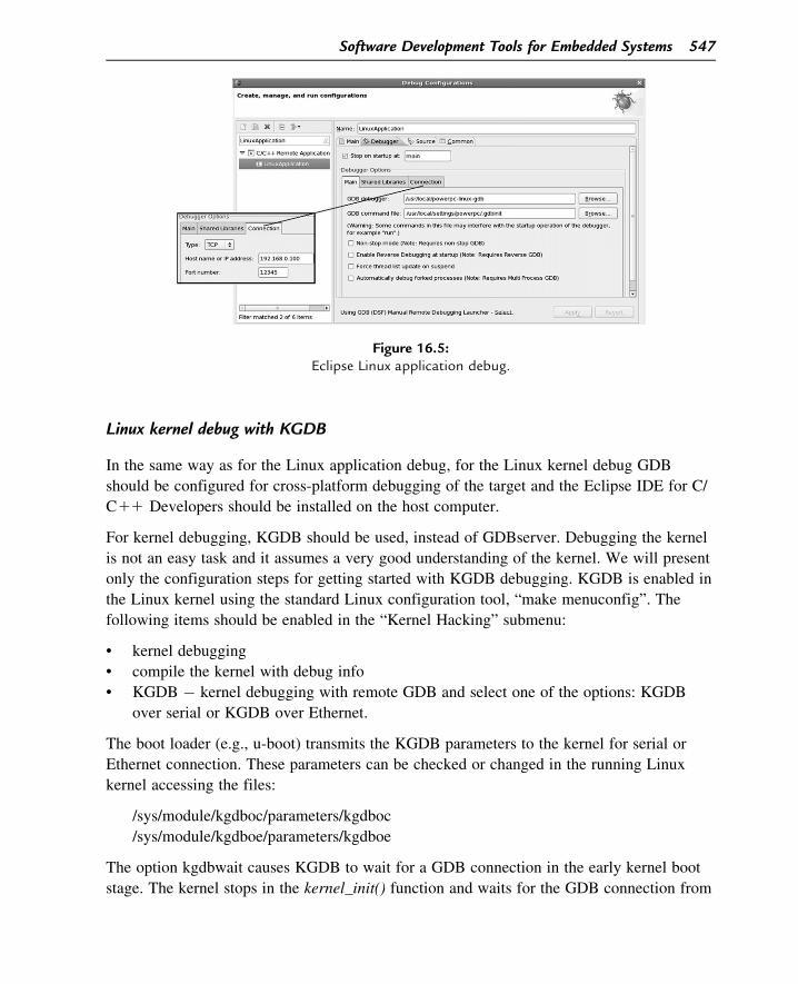
Linux kernel debug with KGDB

In the same way as for the Linux application debug, for the Linux kernel debug GDB

should be configured for cross-platform debugging of the target and the Eclipse IDE for C/

C11 Developers should be installed on the host computer.

For kernel debugging, KGDB should be used, instead of GDBserver. Debugging the kernel

is not an easy task and it assumes a very good understanding of the kernel. We will present

only the configuration steps for getting started with KGDB debugging. KGDB is enabled in

the Linux kernel using the standard Linux configuration tool, “make menuconfig”. The

following items should be enabled in the “Kernel Hacking” submenu:

• kernel debugging

• compile the kernel with debug info

• KGDB � kernel debugging with remote GDB and select one of the options: KGDB

over serial or KGDB over Ethernet.

The boot loader (e.g., u-boot) transmits the KGDB parameters to the kernel for serial or

Ethernet connection. These parameters can be checked or changed in the running Linux

kernel accessing the files:

/sys/module/kgdboc/parameters/kgdboc

/sys/module/kgdboe/parameters/kgdboe

The option kgdbwait causes KGDB to wait for a GDB connection in the early kernel boot

stage. The kernel stops in the kernel_init() function and waits for the GDB connection from

Figure 16.5:Eclipse Linux application debug.


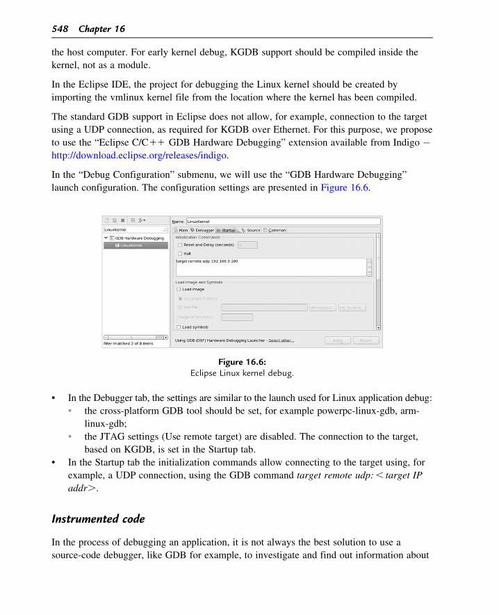
the host computer. For early kernel debug, KGDB support should be compiled inside the

kernel, not as a module.

In the Eclipse IDE, the project for debugging the Linux kernel should be created by

importing the vmlinux kernel file from the location where the kernel has been compiled.

The standard GDB support in Eclipse does not allow, for example, connection to the target

using a UDP connection, as required for KGDB over Ethernet. For this purpose, we propose

to use the “Eclipse C/C11 GDB Hardware Debugging” extension available from Indigo �http://download.eclipse.org/releases/indigo.

In the “Debug Configuration” submenu, we will use the “GDB Hardware Debugging”

launch configuration. The configuration settings are presented in Figure 16.6.

• In the Debugger tab, the settings are similar to the launch used for Linux application debug:

• the cross-platform GDB tool should be set, for example powerpc-linux-gdb, arm-

linux-gdb;

• the JTAG settings (Use remote target) are disabled. The connection to the target,

based on KGDB, is set in the Startup tab.

• In the Startup tab the initialization commands allow connecting to the target using, for

example, a UDP connection, using the GDB command target remote udp:, target IP

addr..

Instrumented code

In the process of debugging an application, it is not always the best solution to use a

source-code debugger, like GDB for example, to investigate and find out information about

Figure 16.6:Eclipse Linux kernel debug.

548 Chapter 16

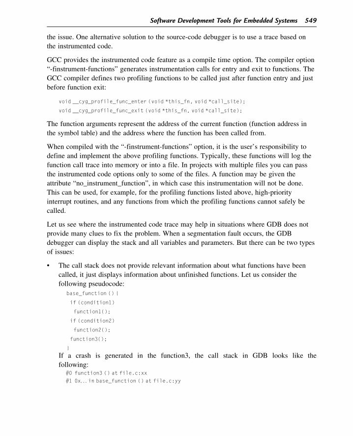
http://download.eclipse.org/releases/indigo

the issue. One alternative solution to the source-code debugger is to use a trace based on

the instrumented code.

GCC provides the instrumented code feature as a compile time option. The compiler option

“-finstrument-functions” generates instrumentation calls for entry and exit to functions. The

GCC compiler defines two profiling functions to be called just after function entry and just

before function exit:

void __cyg_profile_func_enter (void *this_fn, void *call_site);

void __cyg_profile_func_exit (void *this_fn, void *call_site);

The function arguments represent the address of the current function (function address in

the symbol table) and the address where the function has been called from.

When compiled with the “-finstrument-functions” option, it is the user’s responsibility to

define and implement the above profiling functions. Typically, these functions will log the

function call trace into memory or into a file. In projects with multiple files you can pass

the instrumented code options only to some of the files. A function may be given the

attribute “no_instrument_function”, in which case this instrumentation will not be done.

This can be used, for example, for the profiling functions listed above, high-priority

interrupt routines, and any functions from which the profiling functions cannot safely be

called.

Let us see where the instrumented code trace may help in situations where GDB does not

provide many clues to fix the problem. When a segmentation fault occurs, the GDB

debugger can display the stack and all variables and parameters. But there can be two types

of issues:

• The call stack does not provide relevant information about what functions have been

called, it just displays information about unfinished functions. Let us consider the

following pseudocode:

base_function () {

if (condition1)

function1();

if (condition2)

function2();

function3();

}If a crash is generated in the function3, the call stack in GDB looks like the

following:#0 function3 () at file.c:xx#1 0x. . . in base_function () at file.c:yy


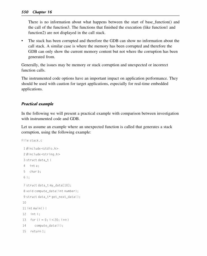
There is no information about what happens between the start of base_function() and

the call of the function3. The functions that finished the execution (like function1 and

function2) are not displayed in the call stack.

• The stack has been corrupted and therefore the GDB can show no information about the

call stack. A similar case is where the memory has been corrupted and therefore the

GDB can only show the current memory content but not where the corruption has been

generated from.

Generally, the issues may be memory or stack corruption and unexpected or incorrect

function calls.

The instrumented code options have an important impact on application performance. They

should be used with caution for target applications, especially for real-time embedded

applications.

Practical example

In the following we will present a practical example with comparison between investigation

with instrumented code and GDB.

Let us assume an example where an unexpected function is called that generates a stack

corruption, using the following example:

File stack.c

1 #include,stdio.h.

2 #include,string.h.

3 struct data_t {

4 int a;

5 char b;

6 };

7 struct data_t my_data[10];

8 void compute_data(int number);

9 struct data_t* get_next_data();

10

11 int main() {

12 int i;

13 for (i 5 0; i,20; i11)

14 compute_data(i);

15 return 1;

550 Chapter 16

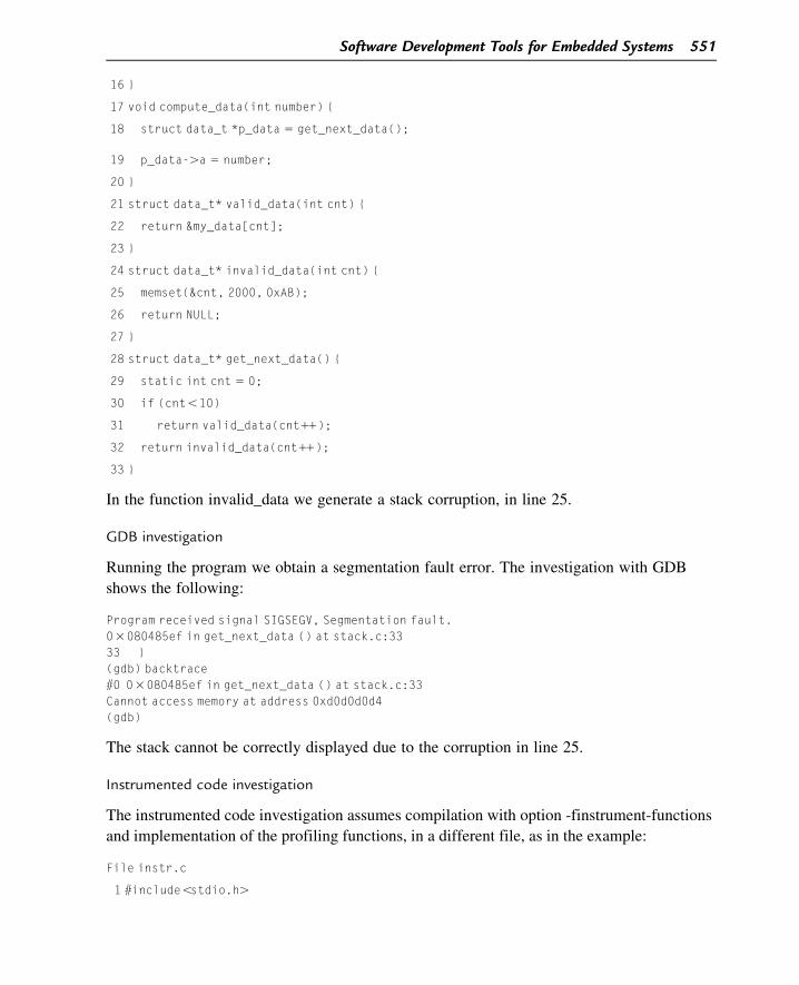
16 }

17 void compute_data(int number) {

18 struct data_t *p_data 5 get_next_data();

19 p_data-.a 5 number;

20 }

21 struct data_t* valid_data(int cnt) {

22 return &my_data[cnt];

23 }

24 struct data_t* invalid_data(int cnt) {

25 memset(&cnt, 2000, 0xAB);

26 return NULL;

27 }

28 struct data_t* get_next_data() {

29 static int cnt 5 0;

30 if (cnt,10)

31 return valid_data(cnt11);

32 return invalid_data(cnt11);

33 }

In the function invalid_data we generate a stack corruption, in line 25.

GDB investigation

Running the program we obtain a segmentation fault error. The investigation with GDB

shows the following:

Program received signal SIGSEGV, Segmentation fault.03080485ef in get_next_data () at stack.c:3333 }(gdb) backtrace#0 03080485ef in get_next_data () at stack.c:33Cannot access memory at address 0xd0d0d0d4(gdb)

The stack cannot be correctly displayed due to the corruption in line 25.

Instrumented code investigation

The instrumented code investigation assumes compilation with option -finstrument-functions

and implementation of the profiling functions, in a different file, as in the example:

File instr.c

1 #include,stdio.h.


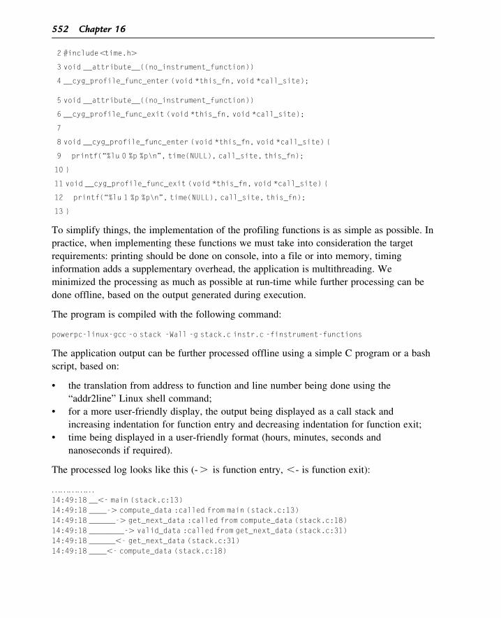
2 #include,time.h.

3 void __attribute__((no_instrument_function))

4 __cyg_profile_func_enter (void *this_fn, void *call_site);

5 void __attribute__((no_instrument_function))

6 __cyg_profile_func_exit (void *this_fn, void *call_site);

7

8 void __cyg_profile_func_enter (void *this_fn, void *call_site) {

9 printf(“%lu 0 %p %p\n”, time(NULL), call_site, this_fn);

10 }

11 void __cyg_profile_func_exit (void *this_fn, void *call_site) {

12 printf(“%lu 1 %p %p\n”, time(NULL), call_site, this_fn);

13 }

To simplify things, the implementation of the profiling functions is as simple as possible. In

practice, when implementing these functions we must take into consideration the target

requirements: printing should be done on console, into a file or into memory, timing

information adds a supplementary overhead, the application is multithreading. We

minimized the processing as much as possible at run-time while further processing can be

done offline, based on the output generated during execution.

The program is compiled with the following command:

powerpc-linux-gcc -o stack -Wall -g stack.c instr.c -finstrument-functions

The application output can be further processed offline using a simple C program or a bash

script, based on:

• the translation from address to function and line number being done using the

“addr2line” Linux shell command;

• for a more user-friendly display, the output being displayed as a call stack and

increasing indentation for function entry and decreasing indentation for function exit;

• time being displayed in a user-friendly format (hours, minutes, seconds and

nanoseconds if required).

The processed log looks like this (-. is function entry, ,- is function exit):

. . .. . .. . .. . .. . .

14:49:18 __,- main (stack.c:13)14:49:18 ____-. compute_data :called from main (stack.c:13)14:49:18 ______-. get_next_data :called from compute_data (stack.c:18)14:49:18 ________-. valid_data :called from get_next_data (stack.c:31)14:49:18 ______,- get_next_data (stack.c:31)14:49:18 ____,- compute_data (stack.c:18)

552 Chapter 16

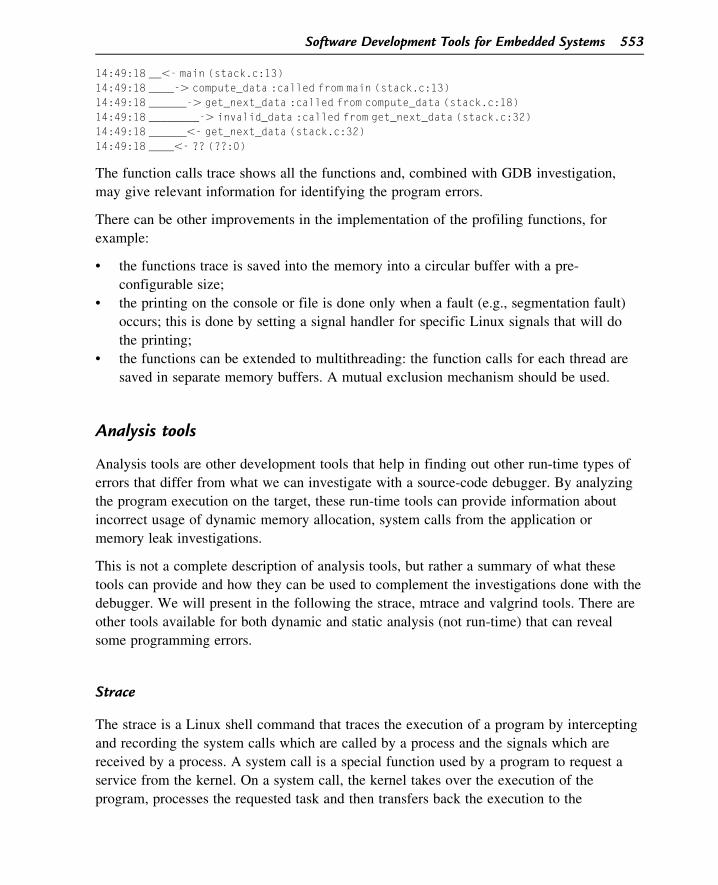
14:49:18 __,- main (stack.c:13)14:49:18 ____-. compute_data :called from main (stack.c:13)14:49:18 ______-. get_next_data :called from compute_data (stack.c:18)14:49:18 ________-. invalid_data :called from get_next_data (stack.c:32)14:49:18 ______,- get_next_data (stack.c:32)14:49:18 ____,- ?? (??:0)

The function calls trace shows all the functions and, combined with GDB investigation,

may give relevant information for identifying the program errors.

There can be other improvements in the implementation of the profiling functions, for

example:

• the functions trace is saved into the memory into a circular buffer with a pre-

configurable size;

• the printing on the console or file is done only when a fault (e.g., segmentation fault)

occurs; this is done by setting a signal handler for specific Linux signals that will do

the printing;

• the functions can be extended to multithreading: the function calls for each thread are

saved in separate memory buffers. A mutual exclusion mechanism should be used.

Analysis tools

Analysis tools are other development tools that help in finding out other run-time types of

errors that differ from what we can investigate with a source-code debugger. By analyzing

the program execution on the target, these run-time tools can provide information about

incorrect usage of dynamic memory allocation, system calls from the application or

memory leak investigations.

This is not a complete description of analysis tools, but rather a summary of what these

tools can provide and how they can be used to complement the investigations done with the

debugger. We will present in the following the strace, mtrace and valgrind tools. There are

other tools available for both dynamic and static analysis (not run-time) that can reveal

some programming errors.

Strace

The strace is a Linux shell command that traces the execution of a program by intercepting

and recording the system calls which are called by a process and the signals which are

received by a process. A system call is a special function used by a program to request a

service from the kernel. On a system call, the kernel takes over the execution of the

program, processes the requested task and then transfers back the execution to the


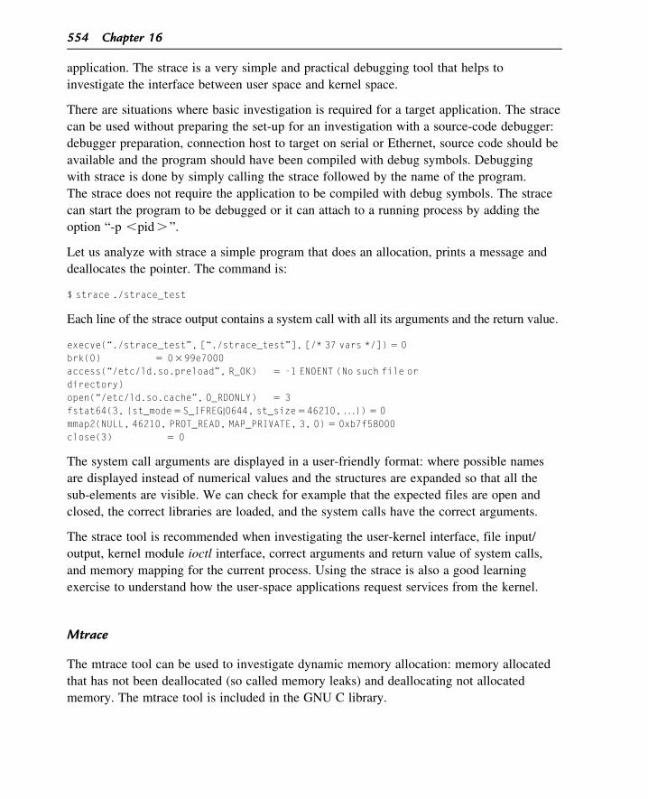
application. The strace is a very simple and practical debugging tool that helps to

investigate the interface between user space and kernel space.

There are situations where basic investigation is required for a target application. The strace

can be used without preparing the set-up for an investigation with a source-code debugger:

debugger preparation, connection host to target on serial or Ethernet, source code should be

available and the program should have been compiled with debug symbols. Debugging

with strace is done by simply calling the strace followed by the name of the program.

The strace does not require the application to be compiled with debug symbols. The strace

can start the program to be debugged or it can attach to a running process by adding the

option “-p ,pid. ”.

Let us analyze with strace a simple program that does an allocation, prints a message and

deallocates the pointer. The command is:

$ strace ./strace_test

Each line of the strace output contains a system call with all its arguments and the return value.

execve(“./strace_test”, [“./strace_test”], [/* 37 vars */]) 5 0brk(0) 5 0399e7000access(“/etc/ld.so.preload”, R_OK) 5 -1 ENOENT (No such file ordirectory)open(“/etc/ld.so.cache”, O_RDONLY) 5 3fstat64(3, {st_mode5S_IFREGj0644, st_size546210, . . .}) 5 0mmap2(NULL, 46210, PROT_READ, MAP_PRIVATE, 3, 0) 5 0xb7f58000close(3) 5 0

The system call arguments are displayed in a user-friendly format: where possible names

are displayed instead of numerical values and the structures are expanded so that all the

sub-elements are visible. We can check for example that the expected files are open and

closed, the correct libraries are loaded, and the system calls have the correct arguments.

The strace tool is recommended when investigating the user-kernel interface, file input/

output, kernel module ioctl interface, correct arguments and return value of system calls,

and memory mapping for the current process. Using the strace is also a good learning

exercise to understand how the user-space applications request services from the kernel.

Mtrace

The mtrace tool can be used to investigate dynamic memory allocation: memory allocated

that has not been deallocated (so called memory leaks) and deallocating not allocated

memory. The mtrace tool is included in the GNU C library.

554 Chapter 16

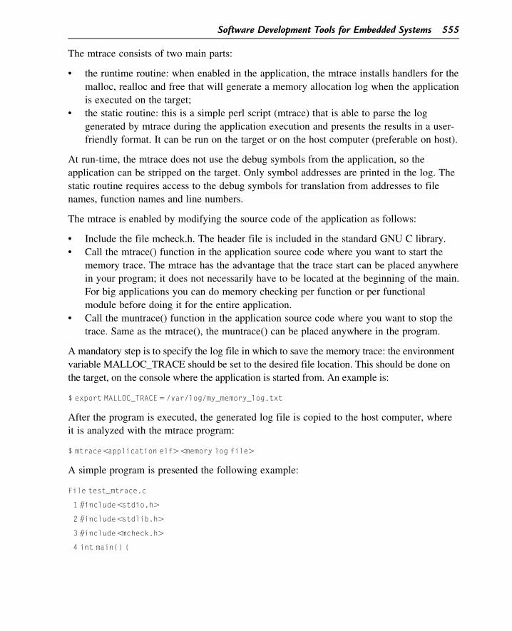
The mtrace consists of two main parts:

• the runtime routine: when enabled in the application, the mtrace installs handlers for the

malloc, realloc and free that will generate a memory allocation log when the application

is executed on the target;

• the static routine: this is a simple perl script (mtrace) that is able to parse the log

generated by mtrace during the application execution and presents the results in a user-

friendly format. It can be run on the target or on the host computer (preferable on host).

At run-time, the mtrace does not use the debug symbols from the application, so the

application can be stripped on the target. Only symbol addresses are printed in the log. The

static routine requires access to the debug symbols for translation from addresses to file

names, function names and line numbers.

The mtrace is enabled by modifying the source code of the application as follows:

• Include the file mcheck.h. The header file is included in the standard GNU C library.

• Call the mtrace() function in the application source code where you want to start the

memory trace. The mtrace has the advantage that the trace start can be placed anywhere

in your program; it does not necessarily have to be located at the beginning of the main.

For big applications you can do memory checking per function or per functional

module before doing it for the entire application.

• Call the muntrace() function in the application source code where you want to stop the

trace. Same as the mtrace(), the muntrace() can be placed anywhere in the program.

A mandatory step is to specify the log file in which to save the memory trace: the environment

variable MALLOC_TRACE should be set to the desired file location. This should be done on

the target, on the console where the application is started from. An example is:

$ export MALLOC_TRACE5/var/log/my_memory_log.txt

After the program is executed, the generated log file is copied to the host computer, where

it is analyzed with the mtrace program:

$ mtrace,application elf.,memory log file.

A simple program is presented the following example:

File test_mtrace.c

1 #include,stdio.h.

2 #include,stdlib.h.

3 #include,mcheck.h.

4 int main() {


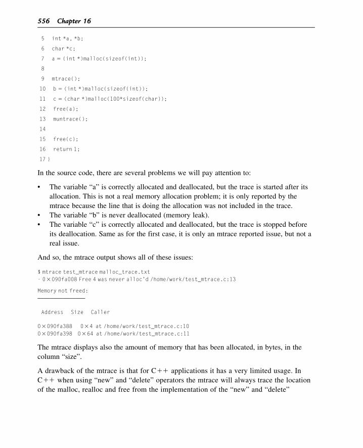
5 int *a, *b;

6 char *c;

7 a 5 (int *)malloc(sizeof(int));

8

9 mtrace();

10 b 5 (int *)malloc(sizeof(int));

11 c 5 (char *)malloc(100*sizeof(char));

12 free(a);

13 muntrace();

14

15 free(c);

16 return 1;

17 }

In the source code, there are several problems we will pay attention to:

• The variable “a” is correctly allocated and deallocated, but the trace is started after its

allocation. This is not a real memory allocation problem; it is only reported by the

mtrace because the line that is doing the allocation was not included in the trace.

• The variable “b” is never deallocated (memory leak).

• The variable “c” is correctly allocated and deallocated, but the trace is stopped before

its deallocation. Same as for the first case, it is only an mtrace reported issue, but not a

real issue.

And so, the mtrace output shows all of these issues:

$ mtrace test_mtrace malloc_trace.txt- 03090fa008 Free 4 was never alloc’d /home/work/test_mtrace.c:13

Memory not freed:———————————————

Address Size Caller

03090fa388 034 at /home/work/test_mtrace.c:1003090fa398 0364 at /home/work/test_mtrace.c:11

The mtrace displays also the amount of memory that has been allocated, in bytes, in the

column “size”.

A drawback of the mtrace is that for C11 applications it has a very limited usage. In

C11 when using “new” and “delete” operators the mtrace will always trace the location

of the malloc, realloc and free from the implementation of the “new” and “delete”

556 Chapter 16

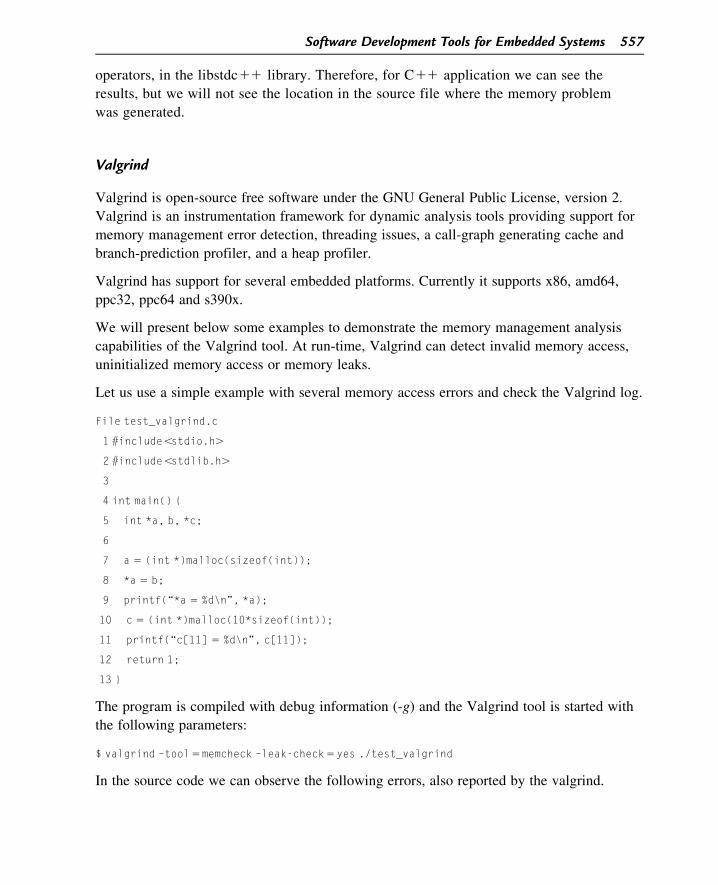
operators, in the libstdc11 library. Therefore, for C11 application we can see the

results, but we will not see the location in the source file where the memory problem

was generated.

Valgrind

Valgrind is open-source free software under the GNU General Public License, version 2.

Valgrind is an instrumentation framework for dynamic analysis tools providing support for

memory management error detection, threading issues, a call-graph generating cache and

branch-prediction profiler, and a heap profiler.

Valgrind has support for several embedded platforms. Currently it supports x86, amd64,

ppc32, ppc64 and s390x.

We will present below some examples to demonstrate the memory management analysis

capabilities of the Valgrind tool. At run-time, Valgrind can detect invalid memory access,

uninitialized memory access or memory leaks.

Let us use a simple example with several memory access errors and check the Valgrind log.

File test_valgrind.c

1 #include,stdio.h.

2 #include,stdlib.h.

3

4 int main() {

5 int *a, b, *c;

6

7 a 5 (int *)malloc(sizeof(int));

8 *a 5 b;

9 printf(“*a 5 %d\n”, *a);

10 c 5 (int *)malloc(10*sizeof(int));

11 printf(“c[11] 5 %d\n”, c[11]);

12 return 1;

13 }

The program is compiled with debug information (-g) and the Valgrind tool is started with

the following parameters:

$ valgrind –tool5memcheck –leak-check5yes ./test_valgrind

In the source code we can observe the following errors, also reported by the valgrind.


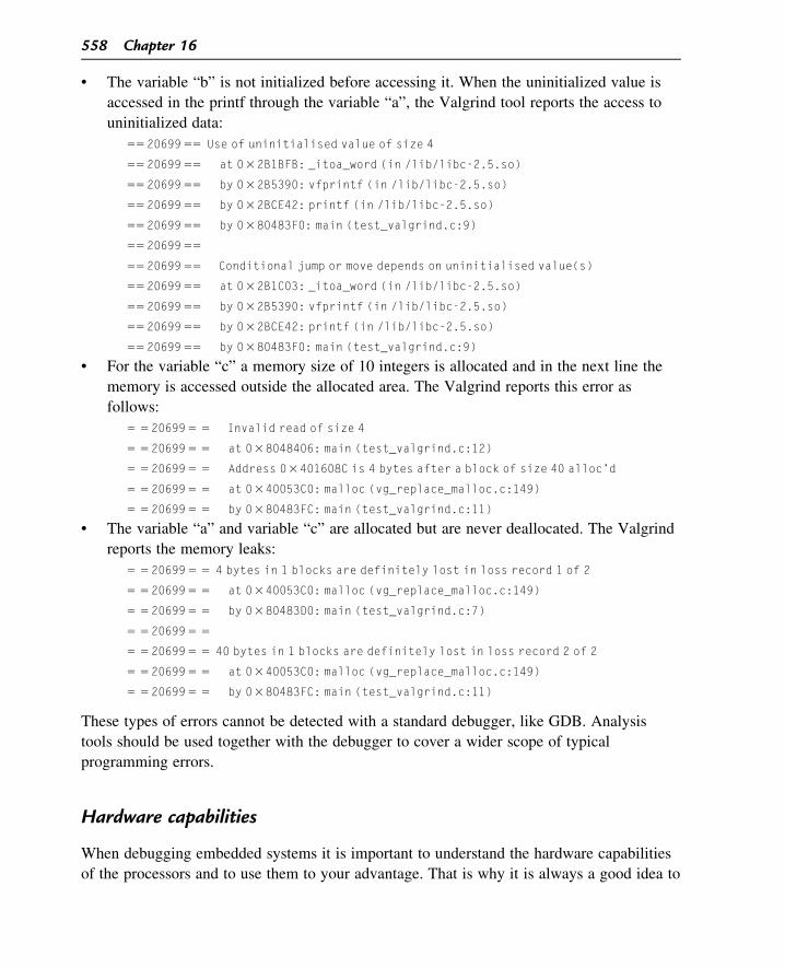
• The variable “b” is not initialized before accessing it. When the uninitialized value is

accessed in the printf through the variable “a”, the Valgrind tool reports the access to

uninitialized data:

552069955 Use of uninitialised value of size 4

552069955 at 032B1BFB: _itoa_word (in /lib/libc-2.5.so)

552069955 by 032B5390: vfprintf (in /lib/libc-2.5.so)

552069955 by 032BCE42: printf (in /lib/libc-2.5.so)

552069955 by 0380483F0: main (test_valgrind.c:9)

552069955

552069955 Conditional jump or move depends on uninitialised value(s)

552069955 at 032B1C03: _itoa_word (in /lib/libc-2.5.so)

552069955 by 032B5390: vfprintf (in /lib/libc-2.5.so)

552069955 by 032BCE42: printf (in /lib/libc-2.5.so)

552069955 by 0380483F0: main (test_valgrind.c:9)

• For the variable “c” a memory size of 10 integers is allocated and in the next line the

memory is accessed outside the allocated area. The Valgrind reports this error as

follows:

5 5206995 5 Invalid read of size 4

5 5206995 5 at 038048406: main (test_valgrind.c:12)

5 5206995 5 Address 03401608C is 4 bytes after a block of size 40 alloc’d

5 5206995 5 at 0340053C0: malloc (vg_replace_malloc.c:149)

5 5206995 5 by 0380483FC: main (test_valgrind.c:11)

• The variable “a” and variable “c” are allocated but are never deallocated. The Valgrind

reports the memory leaks:

5 5206995 5 4 bytes in 1 blocks are definitely lost in loss record 1 of 2


5 5206995 5 by 0380483D0: main (test_valgrind.c:7)

5 5206995 5

5 5206995 5 40 bytes in 1 blocks are definitely lost in loss record 2 of 2


5 5206995 5 by 0380483FC: main (test_valgrind.c:11)

These types of errors cannot be detected with a standard debugger, like GDB. Analysis

tools should be used together with the debugger to cover a wider scope of typical

programming errors.

Hardware capabilities

When debugging embedded systems it is important to understand the hardware capabilities

of the processors and to use them to your advantage. That is why it is always a good idea to

558 Chapter 16

review the processor architecture, features and capabilities and to keep in mind everything

that may help in the debugging process.

Some processors provide a lot of built-in hardware capabilities for debugging, trace and

analysis and profiling. We will refer below to some simple capabilities, but also to more

general ones like hardware breakpoints and hardware watchpoints. Many debuggers have

support for hardware breakpoints or watchpoints. These hardware capabilities do not depend

on the physical debug interface and can work for both debug agent and JTAG probe.

Hardware breakpoints

There are two types of breakpoints: hardware breakpoints based on the processor hardware

capabilities and software breakpoints. For both types of breakpoints, the debugger

apparently takes similar actions. When a breakpoint is added, the debugger needs to know

the address in which to insert the breakpoint. At the user interface, the user can directly

specify the address, the function name or the line number in a source file and, based on the

symbols table, the debugger determines the breakpoint address. When a breakpoint is hit,

for both software and hardware breakpoints, a debug interrupt is generated and the

debugger stops at the breakpoint address. The difference between them is how the debugger

inserts the breakpoint at the required address.

For the software breakpoints, the debugger modifies the program code. The debugger

temporarily stores the instruction located at the breakpoint address and overwrites it with a

special instruction code, specific for each processor. When the program reaches the

breakpoint address, it executes the special instruction that will generate a debug interrupt,

then makes the debugger stop at the breakpoint address. When the breakpoint is removed,

the debugger restores the temporarily saved instruction at the breakpoint address. To step

over a breakpoint, the debugger removes the breakpoint, executes the instruction at the

breakpoint address and then re-inserts the breakpoint. There is one more trick the debugger

does for software breakpoints. While the breakpoint is enabled, for any read operation

through the debugger to the address where the breakpoint has been set it always returns the

temporarily saved instruction but not what is currently at the breakpoint address. So reading

the memory at the breakpoint address will never return the special breakpoint instruction.

There is no limitation in the number of software breakpoints � it depends only on how many

breakpoints are allowed in the debugger software. The software breakpoint is an intrusive

method: it always modifies the code and for this purpose the debugger should have write

access to the breakpoint address. From this comes the software breakpoint limitation: it

cannot be used when the program is running from a read-only location (like ROM or flash).

On the other hand, the hardware breakpoints depend on the hardware capabilities of the

processor. In general processors have some dedicated registers for hardware breakpoints. To


insert a hardware breakpoint, the debugger writes the breakpoint address in one of these

dedicated registers. The rest is done by the processor: when the instruction at that address is

executed, a debug interrupt is generated and the control is transferred to the debugger. The

number of hardware breakpoints is limited by the number of dedicated registers available in

the processor, typically two or four.

Hardware watchpoints

Watchpoints are also named data breakpoints and differ from breakpoints by address use.

For breakpoints, the address represents the code address that, when it is executed, triggers

the debug interrupt. For watchpoints, the address represents a memory address that, when it

is accessed by a read or write operation, triggers the debug interrupt. Therefore, while

breakpoints refer to code addresses, functions and line numbers, watchpoints refer to

memory or data addresses and variable addresses.

A watchpoint is used to stop the execution of the program whenever the watchpoint address is

read from or written to. If the watchpoint is set to a variable, then, the same as for breakpoints,

the debugger translates the variable to an address based on the debug symbol table.

Software watchpoints have no hardware support and therefore it is the debugger that does

the complete handling. A debugger implements a software watchpoint by single-step

running of the program and checking whether the value of the address has been changed

after each step. This is extremely inefficient and it has a significant impact on performance.

Sometimes it may be worth using software watchpoints just to have an idea about which

part of the program corrupts a memory address.

Hardware watchpoints depend on the hardware capabilities of the processor. As for

breakpoints, the processors have dedicated registers for hardware watchpoints. When a

hardware watchpoint is set, one of these registers is set with the watchpoint address,

specifying also the access type: read, write or read-write. For a watchpoint we can specify

the memory zone, not only a single address. For this case, the start and the end address of

the memory are set in the watchpoint registers. The hardware watchpoints have no impact

on performance and therefore it is always recommended to use hardware instead of

software watchpoints, if the processor supports it. The number of hardware watchpoints is

limited by the number of watchpoint registers of the processor.

Debugging tips and tricks

Debugging is a problem-solving process for which it is required to have knowledge,

methodology, intuition, patience and many ideas. Here are some ideas that might help you

in the debugging process.

560 Chapter 16

• If the release application has not been compiled with debug information you can still

debug it. For some compilers like GCC, adding the debug information does not change

symbol values as compared with compilation without -g. In the debugger you should

load the ELF file with debug symbols while debugging the target with the release

application. In the same way you can analyze the core dump created by the release

application.

• For the release application it is always a good idea to enable the core dump even when

the application is stripped. In the case of an application crash you can get the core and

analyze it offline. This is useful especially for applications in the field where you

cannot connect directly with the debugger.

• It is not necessary to enable core dump generation for the entire system. You can

enable it from the application’s source code, as in the example below:

struct rlimit set;

set.rlim_cur 5 0xFFFFFFFF;

set.rlim_max 5 0xFFFFFFFF;

setrlimit(RLIMIT_CORE, &set);

• When you want to generate a core dump, make sure you do not have a Linux signal

handler defined for the error signals. This will overwrite the default handler so the core

dump is not generated.

• To handle an application crash in a reliable way, you can create an application

supervisor. The supervisor checks whether the application is still alive, and if it has

crashed it will restart it so the down-time will be minimal. You can extend it to watch-

dog services to check whether the application is blocked, not just crashed.

• You can save a snapshot of the application state into a core dump. Of course the core

dump should be enabled. This is useful when the application is blocked and is not

responding (in a deadlock for example) and you cannot connect directly with the

debugger (e.g., the application is running in the field). The solution is to restart the

application, saving its entire state into a core dump. If you send an error signal to the

application, the application will terminate, generating a core dump. You can then get

the core dump and analyze it off line with the debugger. The core dump is created with

the command:

$ kill -SIGSEGV,application pid.

• We can extend the previous idea to the following: at any time you can get some status

information from the application using the Linux signal. This is useful if the application

does not have a management interface (CLI, telnet). In the application, you have to

overwrite the default signal handler for a signal (e.g., SIGUSR1) and use this handler to

provide some status information. The status is dumped by sending the overwritten

signal to the application (kill � SIGUSR1 ,application pid.).

• For real-time applications (e.g., bare-board applications with no operating system) the

debugger is not always a good solution. Even printf messages on the console can be


time-consuming and may affect the real-time functionality of the program. For these

applications it is worth using an oscilloscope. Use the GPIO to trigger different events

to the oscilloscope. You can also use it for profiling functions on interrupt routines: a

GPIO level is set to high when at routine entry and set to low at routine exit. On the

oscilloscope you can see the time duration and the occurrence rate. With more GPIO

pins, you can see the distribution in time of different routines.

• For real-time applications, debug information should be captured in some special

conditions. If some interrupts occur during the debug information capture, the data may

be corrupted or irrelevant. For example, this may happen when you want to correlate

some counters (receive and transmit bytes or packets). So before capturing the data, it

may be necessary to disable interrupts and to enable them again once the capture

is finished.

• Access to memory is the fastest way to store data. For real-time applications, sending

the debug data to the host computer while the application is running may affect the

application functionality. In this case, the debug data can be stored in memory and then

can be retrieved and analyzed later on, offline.

• In the development and debugging process you should pay attention to all of the

following: compiler (check all the warnings), static analysis tools, runtime analysis

tools (e.g., memory management tools) and the debugger.

562 Chapter 16

software engineering for embedded systems || software development tools for embedded systems

Documents