sobie : proceedings of annual meetings 2017
TRANSCRIPT
0
SOBIE : PROCEEDINGS OF
ANNUAL MEETINGS
2017
Compiled and Edited by:
Dr. Vivek Bhargava
Florida Gulf Coast University

SOBIE 2017
1
Proceedings of the Society of Business, Industry and
Economics (SOBIE) Annual Meetings
April 19-21, 2017
Destin, Florida
PAPERS
Technology Certifications and Case Study Where Core Microsoft Office Specialist
Certification in Excel is an Accounting Major Requirement for Graduation……………………..3
Gary G. Johnson and Lori K. Mueller
Tax Yield vs. Marginal Tax Rates: History and Correlation ……………………...………...…..21
Richard Cobb, William T. Fielding and Michael B. Marker
Financing Versus Other Input Costs: The Case of Iowa Agriculture Producers………..………...35
Robert Preston, John E. Peterson and Todd Muehler
Are College Football Betting Markets Efficient? Evidence From Interconference Play……….51
Evan Moore and James Francisco
Teaching Students the Financial Statement Impact of the New Lease Standard……………………….60 Amanda Paul, Richard Turpin and Steve Grice
The Effects of Marketing Strategy on Consumer’s Happiness: Does Marketing Help Consumer’s
Happiness at all?…………………………………………………………………………...…….66 Sungwoo Jung
Awareness Regarding Better Business Bureaus and Chambers of Commerce among College
Students: A Concern for Business Schools?……………………………………………..……..70
Avinash Waikar, Susan Zee, Lillian Yee-Man Fok and Kenneth J. Lacho
ERM Framework: Where We Began……………………………………………………………78
Elizabeth M. Pierce and James Goldstein
High-risk Occupations: The Influence of Crisis Events on Stress and Burnout among Police….90
Lisa M. Russell and Brooklyn Cole
Duopoly, Privatization and Environment………………………………………………………109
Manabendra Dasgupta and Seung Dong Lee

SOBIE 2017
2
ABSTRACTS
Social Media: Education to Business………………….…………………………………...…...120
William Piper and Pj Forrest
$ports $ponsorship: Big Money…………………………………………………………….......123
Pj Forrest
The Role of Foundations in Entrepreneurial Activities …………………………..……………126
Eren Ozgen
Female Entrepreneurs In Developing Countries: What Could Be Possible Challenges?………127
Eren Ozgen
Personal Knowledge Management (PKM) and the Leadership Development of African-
American Women Leaders: A Narrative Inquiry…………………………………………….....128
Kimberly L. Wright

SOBIE 2017
3
Technology Certifications and Case Study Where Core
Microsoft Office Specialist Certification in Excel is an Accounting
Major Requirement for Graduation
Gary G. Johnson, Ph.D., Southeast Missouri State University
Lori K. Mueller, Ed.D., Southeast Missouri State University
Abstract
In this paper we provide a summary of post-undergraduate technology certifications and
present a case study of Microsoft Office Specialist certification in Excel 2013 at a Midwestern
state university. Our research finds each of the certifications has three basic requirements –
education, examination, and experience – and the demand for technology-skilled college
graduates is high. Further, we chronicle the process and outcomes relating to a business school’s
decision to make technology certification, and specifically Excel, a priority.
Introduction
Technology-based certifications available to career-minded accountants have increased at
an increasing rate over the past twenty-five years. Triggering this increase is the profession’s
demand for more tech-savvy personnel, specialization within industries, and major events such
as the Enron scandal, the real estate bubble, and retiring baby boomers. Clearly, accounting has
gone through many changes in recent years requiring increased knowledge/skills/abilities for
those pursuing and within the profession.
According to the American Institute of Certified Public Accountants (“Fundamental Core
Competencies” 2016), “Technology is pervasive in the accounting profession. Individuals
entering the accounting profession must acquire the necessary skills to use technology tools
effectively and efficiently. These technology tools can be used both to develop and apply other
functional competencies.”
Purpose
The purpose of this paper is twofold: (1) highlight the importance of certifications in
general and technology certifications for accountants in particular, and (2) present a case study to
illustrate how business schools might use technology certification as a branding opportunity.
SOBIE 2017
4
Background
Accounting educators are often criticized for not preparing entry-level accountants
sufficiently. This criticism may be warranted, but considering the breadth and depth of
accounting rules, auditing standards, tax changes, big data, and technology advancements, it is
understandable that most undergraduate programs can do little more than introduce the sub-
disciplines of accounting and equip their majors with basics in technology.
“New Age” technologies are creating higher demands on businesses and their workers.
Accounting technologies continue to be at the top of technology rankings (“ISACA” 2016).
Today, accountants are assisted by sophisticated software when recording transactions,
organizing data, tracking inventory, preparing tax returns, and auditing financial statements.
Computer systems make information timelier for accountants and other users of accounting data.
Meanwhile, auditors are able to base their opinions on actual, real-time data. Data extraction
software, such as ACL (Audit Command Language), and IDEA make statistical analysis of data
patterns as easy as a few keystrokes.
In 2004, the U.S. Department of Labor reported that accountants were focusing more
sharply on technology due to the technological demands of their clients and commerce in
general. Since that time the pace has accelerated as an increasing number of accountants and
auditors are equipping themselves with extensive computer skills to meet the marketplace
demand for specialization in correcting problems using software, developing software to meet
unique data management and analytical needs, and in protecting company data via cybersecurity.
More pronounced today is the declaration of Shafer that technological developments have
decreased the number of lower-level accounting positions, while at the same time allowing
accounting systems to not be constrained by time or cost (Shafer 1998).
To address the need for tech savvy business school graduates, universities are beefing up
their technology requirements. Third party attestation via basic certification is becoming a
reality for collegians, especially in the accounting area. Examples include Excel, QuickBooks,
ACL, IDEA, and Peachtree.
Certification Requirements
There are three basic requirements for almost all certifications: education, experience,
and examination. These requirements are not only found in accounting certifications and
licensures, but also in certifications throughout other professions, such as law and medicine. The
use of the three requirements is to ensure high quality candidates, strong association of members,
and baseline protection of the public.
Education

SOBIE 2017
5
Formal education is often the basis for accounting knowledge and skill that positions an
accountant for continuous learning throughout their life and career. Most degree programs
provide the opportunity for accounting students to develop oral, written, and interpersonal skills,
along with exposure to the technical and practical skills needed as they transition to the
workplace. Accounting educators in recent years have focused on communication and team
work skills. Although the coursework completed in obtaining an accounting degree is necessary,
it is merely a foundation accountants can later use to reach their career goals (Hutchinson &
Fleischman 2003).
Examination
Similar to university coursework, exams are used to verify that the individual has
obtained the knowledge necessary to complete the tasks at hand and is able to apply the
knowledge to simulated situations. Each of the certifications discussed in this paper requires
candidates to pass an examination. Most often a passing grade is seventy or seventy-five percent
or higher, and exams are often administered in two or more parts. Allowing candidates to take
the exam in sections enables the individual to focus on a condensed amount of material. For
some certifications, retests are available and often have no effect on the candidate’s end result
(Hutchison & Fleischman 2003).
Experience
The experience requirement is in place to verify that candidates have “real life” know-
how. Practice within the field itself is an important part of learning any trade or skill.
Individuals should learn the relevant information necessary, but applying the rules and
knowledge successfully is equally important. Most certifications have a minimum of two years
of related experience before a candidate can receive the certification, and in the case of the CPA,
a license to practice. This period of field work also allows the candidate to evaluate if they enjoy
the specific area in which they are becoming certified.
Certifications Overview
Numerous certifications are available to accounting professionals. According to Foote,
there are three reasons to pursue certification: (1) special knowledge in a specific area enhances
career opportunities, (2) special training costs associated with being credentialed are justified,
and (3) rewards are available through promotions and pay increases (Foote 2003). Amstutz
reports, “According to the latest Salary Guide from Robert Half, starting salaries for
professionals holding graduate degrees or accounting certifications can be 5 to 15 percent more
than the market average” (Amstutz 2016).
Accountants and auditors are expanding their services to include budget analysis,
financial and investment planning, information technology consulting, and limited legal service
SOBIE 2017
6
(U.S. Department of Labor 2004). The addition of more specialized designations distinguishes
accountants in these and other nontraditional growth areas of accounting. Pragmatically, the
following categories capture the essence of the various accounting certifications: technology,
business/management, finance, general accounting, and government. The focus in this study is
on technology.
Technology
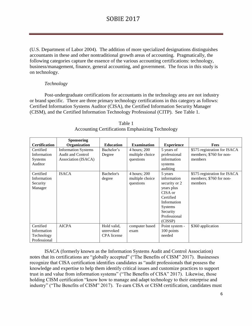
Post-undergraduate certifications for accountants in the technology area are not industry
or brand specific. There are three primary technology certifications in this category as follows:
Certified Information Systems Auditor (CISA), the Certified Information Security Manager
(CISM), and the Certified Information Technology Professional (CITP). See Table 1.
Table 1
Accounting Certifications Emphasizing Technology
Certification
Sponsoring
Organization Education Examination Experience Fees
Certified
Information
Systems
Auditor
Information Systems
Audit and Control
Association (ISACA)
Bachelor’s
Degree
4 hours; 200
multiple choice
questions
5 years of
professional
information
systems
auditing
$575 registration for ISACA
members; $760 for non-
members
Certified
Information
Security
Manager
ISACA Bachelor's
degree
4 hours; 200
multiple choice
questions
5 years
information
security or 2
years plus
CISA or
Certified
Information
Systems
Security
Professional
(CISSP)
$575 registration for ISACA
members; $760 for non-
members
Certified
Information
Technology
Professional
AICPA Hold valid,
unrevoked
CPA license
computer based
exam
Point system -
100 points
needed
$360 application
ISACA (formerly known as the Information Systems Audit and Control Association)
notes that its certifications are “globally accepted” (“The Benefits of CISM” 2017). Businesses
recognize that CISA certification identifies candidates as “audit professionals that possess the
knowledge and expertise to help them identify critical issues and customize practices to support
trust in and value from information systems” (“The Benefits of CISA” 2017). Likewise, those
holding CISM certification “know how to manage and adapt technology to their enterprise and
industry” (“The Benefits of CISM” 2017). To earn CISA or CISM certification, candidates must
SOBIE 2017
7
pass the appropriate exam, complete an application for certification, and agree to adhere to the
code of professional ethics and a continuing professional education program (“How to Become
CISA Certified” 2017, “How to Become CISM Certified” 2017).
According to AICPA, the CITP certification is one of the most popular certifications in
accounting. “A CITP is a CPA credentialed as a technology professional and recognized for
his/her unique ability to bridge between business and technology” (“Certified Information
Technology Professional” 2016). Only CPA members of the AICPA can be CITPs, which
distinguishes these professionals even further. In order to acquire the CITP, an applicant must be
a member in good standing of the AICPA, hold a valid and unrevoked CPA license issued by a
legally constituted state authority, sign a Declaration and Intent to comply with all the
requirements for recertification, complete the CITP application and receive an evaluated score of
at least 100 points, be able to submit up to three references to substantiate business experience in
tech related services, and pay a CITP application fee of $360 (“CITP Application FAQ” 2016).
As highly-focused technologies become an ever more integral part of everyday business
operations, it follows that IT certifications will become more and more important. College
students do not qualify for IT certifications since they require a degree and experience.
However, students can leverage their understanding of technology by becoming Microsoft
certified in Excel which does not require either a college degree or experience. Most agree that
spreadsheet software is the foundation technology for business professionals, especially
accountants. Microsoft Excel is the leading product. Three levels of Microsoft Office Specialist
(MOS) certifications are available for Excel 2013 via a testing program offered through
Microsoft and administered by Certiport (“MOS 2013 Master Certification” 2016). Candidates
who pass the core certification exam receive MOS 2013 certification in Excel (“MOS 2013
Master Certification” 2016). Candidates seeking higher levels of certification may earn MOS
2013 Expert certification in Excel or MOS 2013 Master certification (“MOS 2013 Master
Certification” 2016). Expert certification requires completion of two exams; candidates must
pass both to earn the certification (“MOS 2013 Master Certification” 2016). Master certification
requires completion of a total of four exams; three different “tracks” are available (“MOS 2013
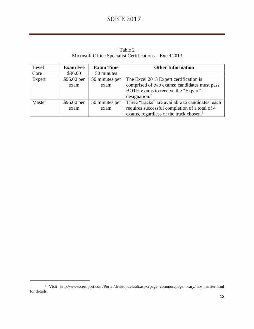
Master Certification” 2016). General information is shown in Table 2.

SOBIE 2017
8
Table 2
Microsoft Office Specialist Certifications – Excel 2013
Level Exam Fee Exam Time Other Information
Core $96.00 50 minutes
Expert $96.00 per
exam
50 minutes per
exam
The Excel 2013 Expert certification is
comprised of two exams; candidates must pass
BOTH exams to receive the “Expert”
designation.1
Master $96.00 per
exam
50 minutes per
exam
Three “tracks” are available to candidates; each
requires successful completion of a total of 4
exams, regardless of the track chosen.1
The value of Excel certification while still a student is non-debatable. Students achieving
Excel certification help themselves in the job search by reducing career risk, the risk they will
graduate and not be professionally employed.
Students entering the job market most likely have no connection with the companies to
which they apply. Therefore, recruiters given only the standard statement “proficient in Excel”
on a resume are not impressed since nearly all students make that claim. Being Microsoft
certified provides prospective employers with the needed third party assurance of the applicant’s
basic technology understanding and skill. In addition, the exam material gives something
technical to be discussed during the interview – a big plus, especially for an accounting major!
According to CompTIA, MOS certification can bring about a 9% increase in starting salary and
may enhance future increases by as much as 29% (“CompTIA Certifications” 2017). Moreover,
an article by Bhargav reports that employers are more comfortable hiring a certified candidate
even if they have to pay a higher salary. In summary, Excel certification means “better
marketability, better recognition and better pay” (Bhargav 2012).
Case Study: Process and Timeline
The need for spreadsheet proficiency in accounting graduates is not new. Academic
programs work to develop these skills in their students, but in most cases without a clear
strategy. In a Midwestern state university (referred to as “the University” in the case
presentation), the accounting faculty in the college of business (referred to as “the College”)
stepped up and now requires third-party certification in the form of the core MOS Excel exam
for all accounting graduates. This cost transfer and skill assurance is well-received by employers
and the general external community. It is a “win-win-win” for the accounting program, students,
and the employer community.
1 Visit http://www.certiport.com/Portal/desktopdefault.aspx?page=common/pagelibrary/mos_master.html
for details.

SOBIE 2017
9
The University is an official test center for MOS certification exams. The University has
been administering MOS exams since 2001, when the College pioneered the practice of offering
workshops to help its students review content and prepare to take the MOS exam for Excel. In
fall 2014, the exam preparation materials were modified to more closely align with the exam
objectives for the core MOS exam for Excel (“Objective Domain” 2014; see Appendix A), and
practice test software from GMetrix was purchased.
The annual fee for a block of 500 exams is $4,200.00 and the fee for the site license from
GMetrix is $4,500.00. The practice test software is available on any University-owned
computer, giving students access to the software as they practice and prepare to take the MOS
exam. Time for students to complete one GMetrix practice test during the face-to-face
workshops was built-in to the process.
Table 3
MOS Excel Cost and Procedures Charges, 2014-2017
Date
Cost for exam site license
(Certiport, 500 exams, annual fee)
Cost for practice test site
license (GMetrix, annual fee)
December 2014 $4,500.00
February 2015 $4,200.00
December 2015 $4,200.00 $4,500.00
December 2016 $4,200.00 $4,500.00
As part of the transition, a course page was developed on Moodle, the University’s
learning management system, for students to participate in a series of workshops. On the
Moodle page, information is provided for students including instructions on how to create a
Certiport account, how to access the GMetrix practice test software, and resources, such as step-
by-step instructions and videos on how to perform different tasks in Excel (e.g., “Excel 2013”
2016; “Basic Tasks in Excel 2013” 2016), PowerPoint presentations with the covered content,
and sample Excel files for students to use to practice tasks and skills in Excel. Students pay $45
per exam administration, a significant savings over the individual voucher cost of $96 through
Certiport (“Shop Products” 2014).
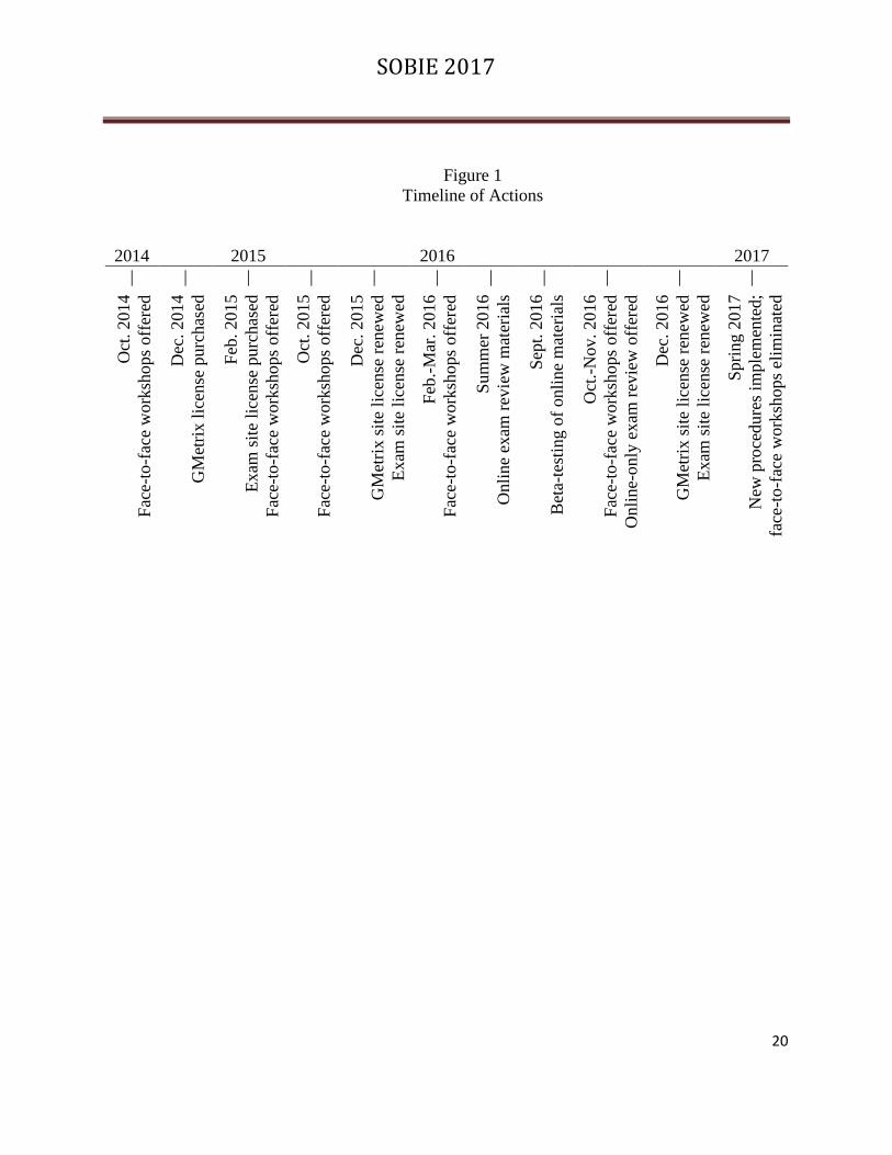
An online-only option for students to review materials in preparation for the MOS exam
in Excel was created in 2016. To accomplish this, the existing Moodle course page was
expanded by using Camtasia to add screen-casting videos. The videos, 22 in all, with a total
running time of approximately 2.5 hours, cover the same content as the face-to-face workshops.
SOBIE 2017
10
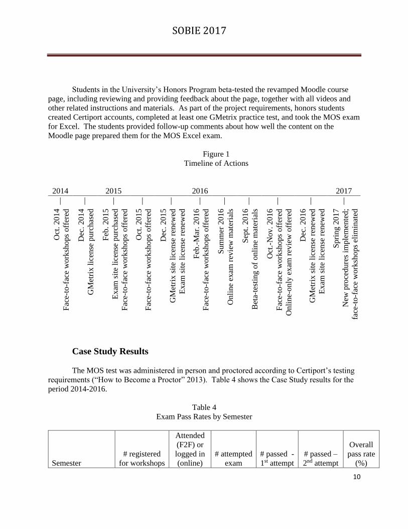
Students in the University’s Honors Program beta-tested the revamped Moodle course
page, including reviewing and providing feedback about the page, together with all videos and
other related instructions and materials. As part of the project requirements, honors students
created Certiport accounts, completed at least one GMetrix practice test, and took the MOS exam
for Excel. The students provided follow-up comments about how well the content on the
Moodle page prepared them for the MOS Excel exam.
Figure 1
Timeline of Actions
2014 2015 2016 2017
| | | | | | | | | | |
Oct
. 2014
Fac
e-to
-fac
e w
ork
shops
off
ered
Dec
. 2014
GM
etri
x l
icen
se p
urc
has
ed
Feb
. 2015
Exam
sit
e li
cense
purc
has
ed
Fac
e-to
-fac
e w
ork
shop
s off
ered
Oct
. 2015
Fac
e-to
-fac
e w
ork
shops
off
ered
Dec
. 2015
GM
etri
x s
ite
lice
nse
ren
ewed
Exam
sit
e li
cense
ren
ewed
Feb
.-M
ar. 2016
Fac
e-to
-fac
e w
ork
shops
off
ered
Sum
mer
2016
Onli
ne
exam
rev
iew
mat
eria
ls
dev
eloped
S
ept.
2016
Bet
a-te
stin
g o
f onli
ne
mat
eria
ls
Oct
.-N
ov. 2016
Fac
e-to
-fac
e w
ork
shops
off
ered
Onli
ne-
only
exam
rev
iew
off
ered
Dec
. 2016
GM
etri
x s
ite
lice
nse
ren
ewed
Exam
sit
e li
cense
ren
ewed
Spri
ng 2
017
New
pro
cedure
s im
ple
men
ted;
face
-to-f
ace
work
shops
elim
inat
ed
Case Study Results
The MOS test was administered in person and proctored according to Certiport’s testing
requirements (“How to Become a Proctor” 2013). Table 4 shows the Case Study results for the
period 2014-2016.
Table 4
Exam Pass Rates by Semester
Semester
# registered
for workshops
Attended
(F2F) or
logged in
(online)
# attempted
exam
# passed -
1st attempt
# passed –
2nd attempt
Overall
pass rate
(%)

SOBIE 2017
11
Fall 2014 47 29 23 15 6 91%
Spring 2015 41 28 28 21 2 82%
Fall 2015 56 36 29 23 3 90%
Spring 2016 58 35 28 22 1 82%
Fall 2016 (F2F) 16 12 10 10 N/A 100%
Fall 2016 (online) 26 24 10 9 1 100%
Going Forward
Beginning with spring 2017, the College plans to eliminate the face-to-face workshops.
Students in the College will be provided with information on how to self-enroll in the Moodle
course page containing the MOS exam review materials. They will be able to review at their
own pace as is convenient with their individual schedules. They will continue to have access to
the GMetrix software, and can take practice tests on any University computers. Instead of only
being able to test at set times related to the dates of the face-to-face workshops, students will be
able to schedule individual appointments with the University’s testing services department and
test whenever they feel ready to take the exam.
Conclusions
John Radford, CGFM, Controller for the State of Oregon, summed up accounting
certifications, “In today’s complex and changing world, a professional certification provides
employers with a degree of confidence that candidates are prepared for the real world” (“CGFM”
2017).
Requiring technology certification of graduates represents a good “branding” strategy for
a business school. Moreover, given the significant demand for technology-savvy business
graduates, it seems logical that getting a head start on a technology certification while a student
is a great strategy. Colleges of business may assist these students by establishing and requiring a
basic third-party technology certification, such as Microsoft Office Certification in Excel, of
their business graduates.
REFERENCES
Amstutz, L. “Accounting and Financial Certifications Employers Want to See.” Robert Half
Finance & Accounting. Last modified August 4, 2016.
https://www.roberthalf.com/finance/blog/accounting-and-financial-certifications-
employers-want-to-see.
“Basic Tasks in Excel 2013.” Microsoft, 2016. Accessed September 13, 2016.
https://support.office.com/en-us/article/Basic-tasks-in-Excel-2013-363600c5-55be-4d6e-
SOBIE 2017
12
82cf-b0a41e294054?CorrelationId=0690568e-79a1-4378-8af1-dceac8cccb8d&ui=en-
US&rs=en-US&ad=US&ocmsassetID=HA102813812.
Bhargav, R. “Role of Microsoft Excel Certification in Your Career.” SimpliLearn. Last
modified May 26, 2012. https://www.simplilearn.com/role-of-microsoft-excel-
certification-in-your-career-rar270-article.
“Certified Information Technology Professional (CITP) Credential Overview.” American
Institute of Certified Public Accountants, 2016. Accessed January 14, 2017.
http://www.aicpa.org/Membership/Join/Pages/CITP-Credential-Canada.aspx.
“CGFM – the Mark of Excellence in Federal, State, and Local Government.” Association of
Government Accountants, 2017. Accessed January 12, 2017.
https://www.agacgfm.org/Chapters/CentralArkansas/CGFM-Certification.aspx.
“CITP Application FAQ.” American Institute of Certified Public Accountants, 2016. Accessed
January 14, 2017.
http://www.aicpa.org/interestareas/informationtechnology/membership/pages/citpfaqsapp
l.aspx.
“CompTIA Certifications.” ITCareerFinder, 2017. Accessed January 14, 2017.
http://www.itcareerfinder.com/it-certifications/comptia-certifications.html.
“Excel 2013.” Goodwill Community Foundation, Inc., 2016. Accessed September 13, 2016.
http://www.gcflearnfree.org/excel2013/.
Foote, D. “IT Job Trend Yields Surprises” Computerworld, February 2003, Vol. 37, Issue 6, 23.
“Functional Core Competencies for the Accounting Profession.” American Institute of Certified
Public Accountants, 2016. Accessed January 12, 2017.
https://www.aicpa.org/InterestAreas/AccountingEducation/Resources/Pages/accounting-
core-competencies-functional.aspx.
“How to Become CISA Certified.” ISACA, 2017. Accessed January 14, 2017.
http://www.isaca.org/Certification/CISA-Certified-Information-Systems-Auditor/How-
to-Become-Certified/Pages/default.aspx.
“How to Become CISM Certified.” ISACA, 2017. Accessed January 14, 2017.
http://www.isaca.org/Certification/CISM-Certified-Information-Security-Manager/How-
to-Become-Certified/Pages/default.aspx.
SOBIE 2017
13
“How to Become a Proctor/Add Proctor to Testing Center.” Certiport, 2013. Accessed
September 13, 2016.
https://www.certiport.com/Portal/common/documentlibrary/Q10_BecomeProctor.pdf.
Hutchison, P. D. and G. M. Fleischman. “Professional Certification Opportunities for
Accountants” The CPA Journal, Mar 2003, Vol. 73, Issue 3, 48-51.
“ISACA.” ISACA, 2016. Accessed October 5, 2016. http://www.isaca.org.
“MOS 2013 Master Certification is Now Easier Than You Thought.” Certiport, 2016. Accessed
December 22, 2016.
http://www.certiport.com/Portal/desktopdefault.aspx?page=common/pagelibrary/mos_ma
ster.html.
“Objective Domain: MOS Excel 2013.” Certiport, 2014. Accessed September 13, 2016.
http://studio-element.com/certiport/mos-excel-objectives.html.
Shafer, W. E. “The Accounting Profession in the New Millennium” Business Forum, 1998, Vol.
23, Issue 1/2, 31-36. Retrieved March 29, 2005, from ProQuest.
“Shop Products.” Certiport, 2014. Accessed September 13, 2016.
http://shop.certiport.com/category-s/1905.htm.
“The Benefits of CISA.” ISACA, 2017. Accessed January 14, 2017.
http://www.isaca.org/Certification/CISA-Certified-Information-Systems-Auditor/What-
is-CISA/Pages/default.aspx.
“The Benefits of CISM.” ISACA, 2017. Accessed January 14, 2017.
http://www.isaca.org/Certification/CISM-Certified-Information-Security-Manager/What-
is-CISM/Pages/default.aspx.
U.S. Department of Labor, Bureau of Labor Statistics. Occupational Outlook Handbook, 2004-
05 Edition. Bulletin 2540.

SOBIE 2017
14
APPENDIX A
OBJECTIVE DOMAIN: MOS EXCEL 2013
1.0 Create and Manage Worksheets and Workbooks
1.1 Create Worksheets and Workbooks
This objective may include but is not limited to: creating new blank workbooks, creating
new workbooks using templates, importing files, opening non-native files directly in
Excel, adding worksheets to existing workbooks, copying and moving worksheets
1.2 Navigate through Worksheets and Workbooks
This objective may include but is not limited to: searching for data within a workbook,
inserting hyperlinks, changing worksheet order, using Go To, using Name Box
1.3 Format Worksheets and Workbooks
This objective may include but is not limited to: changing worksheet tab color, modifying
page setup, inserting and deleting columns and rows, changing workbook themes,
adjusting row height and column width, inserting watermarks, inserting headers and
footers, setting data validation
1.4 Customize Options and Views for Worksheets and Workbooks
This objective may include but is not limited to: hiding worksheets, hiding columns and
rows, customizing the Quick Access toolbar, customizing the Ribbon, managing macro
security, changing workbook views, recording simple macros, adding values to workbook
properties, using zoom, displaying formulas, freezing panes, assigning shortcut keys,
splitting the window
1.5 Configure Worksheets and Workbooks to Print or Save
This objective may include but is not limited to: setting a print area, saving workbooks in
alternate file formats, printing individual worksheets, setting print scaling, repeating
headers and footers, maintaining backward compatibility, configuring workbooks to
print, saving files to remote locations
2.0 Create Cells and Ranges
2.1 Insert Data in Cells and Ranges
This objective may include but is not limited to: appending data to worksheets, finding
and replacing data, copying and pasting data, using AutoFill tool, expanding data across
columns, inserting and deleting cells

SOBIE 2017
15
2.2 Format Cells and Ranges
This objective may include but is not limited to: merging cells, modifying cell alignment
and indentation, changing font and font styles, using Format Painter, wrapping text
within cells, applying Number formats, applying highlighting, applying cell styles,
changing text to WordArt
2.3 Order and Group Cells and Ranges
This objective may include but is not limited to: applying conditional formatting,
inserting sparklines, transposing columns and rows, creating named ranges, creating
outlines, collapsing groups of data in outlines, inserting subtotals
3.0 Create Tables
3.1 Create a Table
This objective may include but is not limited to: moving between tables and ranges,
adding and removing cells within tables, defining titles
3.2 Modify a Table
This objective may include but is not limited to: applying styles to tables, banding rows
and columns, inserting total rows, removing styles from tables
3.3 Filter and Sort a Table
This objective may include but is not limited to: filtering records, sorting data on multiple
columns, changing sort order, removing duplicates
4.0 Apply Formulas and Functions
4.1 Utilize Cell Ranges and References in Formulas and Functions
This objective may include but is not limited to: utilizing references (relative, mixed,
absolute), defining order of operations, referencing cell ranges in formulas
4.2 Summarize Data with Functions
This objective may include but is not limited to: utilizing the SUM function, utilizing the
MIN and MAX functions, utilizing the COUNT function, utilizing the AVERAGE
function
4.3 Utilize Conditional Logic in Functions
This objective may include but is not limited to: utilizing the SUMIF function, utilizing
the AVERAGEIF function, utilizing the COUNTIF function
4.4 Format and Modify Text with Functions
SOBIE 2017
16
This objective may include but is not limited to: utilizing the RIGHT, LEFT and MID
functions, utilizing the TRIM function, utilizing the UPPER and LOWER functions,
utilizing the CONCATENATE function
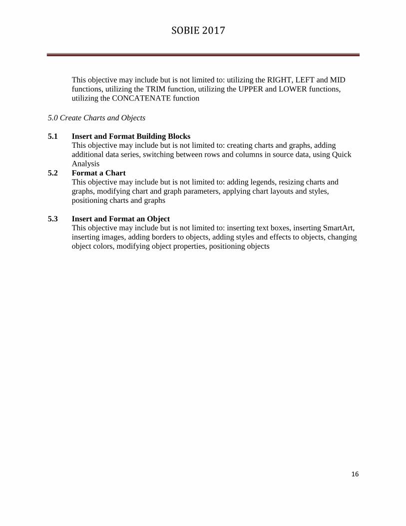
5.0 Create Charts and Objects
5.1 Insert and Format Building Blocks
This objective may include but is not limited to: creating charts and graphs, adding
additional data series, switching between rows and columns in source data, using Quick
Analysis
5.2 Format a Chart
This objective may include but is not limited to: adding legends, resizing charts and
graphs, modifying chart and graph parameters, applying chart layouts and styles,
positioning charts and graphs
5.3 Insert and Format an Object
This objective may include but is not limited to: inserting text boxes, inserting SmartArt,
inserting images, adding borders to objects, adding styles and effects to objects, changing
object colors, modifying object properties, positioning objects

SOBIE 2017
17
Table 1
Accounting Certifications Emphasizing Technology
Certification
Sponsoring
Organization Education Examination Experience Fees
Certified
Information
Systems
Auditor
Information Systems
Audit and Control
Association (ISACA)
Bachelor’s
Degree
4 hours; 200
multiple choice
questions
5 years of
professional
information
systems
auditing
$575 registration for ISACA
members; $760 for non-
members
Certified
Information
Security
Manager
ISACA Bachelor's
degree
4 hours; 200
multiple choice
questions
5 years
information
security or 2
years plus
CISA or
Certified
Information
Systems
Security
Professional
(CISSP)
$575 registration for ISACA
members; $760 for non-
members
Certified
Information
Technology
Professional
AICPA Hold valid,
unrevoked
CPA license
computer based
exam
Point system -
100 points
needed
$360 application
SOBIE 2017
18
Table 2
Microsoft Office Specialist Certifications – Excel 2013
Level Exam Fee Exam Time Other Information
Core $96.00 50 minutes
Expert $96.00 per
exam
50 minutes per
exam
The Excel 2013 Expert certification is
comprised of two exams; candidates must pass
BOTH exams to receive the “Expert”
designation.2
Master $96.00 per
exam
50 minutes per
exam
Three “tracks” are available to candidates; each
requires successful completion of a total of 4
exams, regardless of the track chosen.1
2 Visit http://www.certiport.com/Portal/desktopdefault.aspx?page=common/pagelibrary/mos_master.html
for details.

SOBIE 2017
19
Table 3
MOS Excel Cost and Procedures Charges, 2014-2017
Date
Cost for exam site license
(Certiport, 500 exams, annual fee)
Cost for practice test site
license (GMetrix, annual fee)
December 2014 $4,500.00
February 2015 $4,200.00
December 2015 $4,200.00 $4,500.00
December 2016 $4,200.00 $4,500.00
Table 4
Exam Pass Rates by Semester
Semester
# registered
for workshops
Attended
(F2F) or
logged in
(online)
# attempted
exam
# passed -
1st attempt
# passed –
2nd attempt
Overall
pass rate
(%)
Fall 2014 47 29 23 15 6 91%
Spring 2015 41 28 28 21 2 82%
Fall 2015 56 36 29 23 3 90%
Spring 2016 58 35 28 22 1 82%
Fall 2016 (F2F) 16 12 10 10 N/A 100%
Fall 2016 (online) 26 24 10 9 1 100%
SOBIE 2017
20
Figure 1
Timeline of Actions
2014 2015 2016 2017
| | | | | | | | | | |
Oct
. 2014
Fac
e-to
-fac
e w
ork
shops
off
ered
Dec
. 2014
GM
etri
x l
icen
se p
urc
has
ed
Feb
. 2015
Exam
sit
e li
cense
purc
has
ed
Fac
e-to
-fac
e w
ork
shops
off
ered
Oct
. 2015
Fac
e-to
-fac
e w
ork
shops
off
ered
Dec
. 2015
GM
etri
x s
ite
lice
nse
ren
ewed
Exam
sit
e li
cense
ren
ewed
Feb
.-M
ar. 2016
Fac
e-to
-fac
e w
ork
shops
off
ered
Sum
mer
2016
Onli
ne
exam
rev
iew
mat
eria
ls
dev
eloped
S
ept.
2016
Bet
a-te
stin
g o
f onli
ne
mat
eria
ls
Oct
.-N
ov. 2016
Fac
e-to
-fac
e w
ork
shops
off
ered
Onli
ne-
only
exam
rev
iew
off
ered
Dec
. 2016
GM
etri
x s
ite
lice
nse
ren
ewed
Exam
sit
e li
cense
ren
ewed
Spri
ng 2
017
New
pro
cedure
s im
ple
men
ted;
face
-to-f
ace
work
shops
elim
inat
ed

SOBIE 2017
21
Tax Yield vs. Marginal Tax Rates
History and Correlation
Richard Cobb, Jacksonville State University
William T. Fielding, Jacksonville State University
Michael B. Marker, Jacksonville State University
Abstract
An internet search of marginal tax rates will yield thousands of hits. A casual scan of
these web addresses finds some sites reporting on technical tax issues, while other sites review
political arguments concerning adjusting tax rates to support increased government revenues.
Many of these reports focus on the subjective definition of fair tax planning. Our research uses
an objective approach to analyze the related Bureau of Economic Analysis (BEA) tax data in an
effort to determine the correlation between the principal research variables of tax rates and tax
yield relative to gross domestic product (GDP).
Introduction
When political leaders debate the funding needs of government programs, they must
agree on which sources of funds to use and which funding mechanisms will successfully collect
the funds required. In the early years of our nation, monies collected from tariffs, custom duties,
and specific item taxes were sufficient to meet these government-supported programs. Today the
debate is focused almost exclusively on changing individual and corporate tax rates and tax
brackets in order to meet funding needs. After reviewing the history of changes involving these
tax plans, we find that the highest marginal tax rate has been changed twelve times since World
War II. Although all modern tax plans have been debated, approved, and regulated during this
period, there has been no clear agreement concerning the effect that tax rates have on tax yield
needed to support GDP and economic growth. This research will define tax yield as the
percentage rate of return from tax revenue generated relative to GDP for various changing
marginal tax rates. Our findings will focus on determining the correlation between the research
variables from 1946 forward.
Taxation
Taxation is the dominate method of funding government activities and programs. Today
we understand that the tax scenario proposing to create a fair tax plan is as old as civilization
itself. This notion of fairness can be traced to the principles offered by Adam Smith (1776) in
his book Wealth of Nations. He wrote that taxation should be based, in part, on equity and that
individuals who earn more should pay more to support state services. Barro (2009) recognized
SOBIE 2017
22
this role of the state and wrote that incentives to invest could be supported by state tax policy. He
suggested that the reduction of marginal income tax rates could be an incentive to support
investment. Emphasizing this theme, Hauser (2010) noted that the animal spirits of
entrepreneurship were discouraged by higher taxes. This conclusion was also drawn by Ranson
(2010), who observed that when taxpayers face higher tax rates, they have an incentive to pay
less tax. In the Wall Street Journal (2 August 2010), Arthur Laffer echoed these same concerns
and noted that “the highest tax bracket income earners, when compared with those people in
lower tax brackets, are far more capable of changing their taxable income.” He concluded, for
example, that as higher marginal tax rates were reduced, beginning in the 1970s, tax receipts for
the top 1% of income earners increased from 1.5% of GDP in 1978 to 3.3% of GDP in 2007.
These research examples emphasize the point that tax on income associated with wealth creation
represents the cost of acquiring that income and that the incentive to earn more may be tied to
reducing tax rates.
Tax Revenue and GDP
Numerous research examples present supporting arguments and graphical representations
that stress the importance of tax rates on tax revenue and on changes in GDP. For example,
Hauser (1993, 1996) noted that regardless of the changes to marginal tax rates, U.S. tax revenue
(federal current receipts) has averaged about 19% of the GDP since WWII. This tax-GDP
relationship has been updated through 2016 by the Federal Reserve Bank of St. Louis (FRED)
with a graphical presentation of total federal current receipts as a percent of GDP that yielded
results similar to those of Hauser. The research theme that monitors total federal tax relative to
GDP is also used by the Tax Policy Center (2017) as it tracks revenue as a share (percent) of
GDP for all government sources.
Other organizations have used the tax-GDP relationship as a metric to measure economic
performance. The Organization for Economic Co-Operation and Development OECD (2014)
used tax revenue relative to GDP to measure national performance. The OECD reviewed the
total tax revenue as a percentage of GDP for 34 countries in its study and found that the average
tax revenue as a percent of GDP for this study group was 35.4 percent. OECD reported that in
2012 the minimum revenue yield country was Chile (20.8%) and the maximum yield country
was Denmark (48.0%). For this period, OECD reported that the U.S. average tax revenue was
24.3 percent of GDP. The World Bank (2014) also used tax revenue and GDP to monitor its
defined world development indicators (WDI) and then recorded the results in the appropriate
WDI table. One such table is Tax revenue as a % of GDP. Here, tax revenue refers to all
transfers that are compulsory and collected by central government for public purposes. Based on
the WDI table definition for tax revenue, the U.S. average tax revenue was 11.0% of GDP for
2014.
A subset of the tax-GDP related research is the federal personal current tax as a percent
of GDP. This subset is compiled using Office of Management and Budget (OMB) data and has

SOBIE 2017
23
been recorded by the Tax Policy Center since 1934. Federal personal current tax was also the
focus of the Heritage Foundation (2016) report. This report described the relationship between
top tax rates and individual tax receipts. The Foundation observed that yield from individual tax
receipts tend to be stable over time as top tax rates change and that higher rates might not lead to
higher receipts.
A Question of Correlation
From the research cited, the general consensus is that lower marginal tax rates support
growth in GDP and the rate of revenue collection (yield) tends to be stable over time. The
evidence of GDP growth with lower tax rates does not suggest, however, that a zero marginal
rate would yield ever higher revenue. The data show only that since 1946, tax revenue (i.e. total,
government, and personal taxes) and GDP have increased as marginal tax rates have declined.
Dependent variables are listed in table 1. Variables included are federal current receipts (FCR),
federal personal current tax (FPCT), and gross domestic product (GDP). Also, we include
marginal tax rates (MTR) that are considered to be independent over the study period. The broad
research objective was to study the direction and the strength of the linear relationships between
our study variables listed in table 1.
The question of variable correlation was addressed by Hao Li On (2010) when he
compared tax rate, tax receipts, and GDP. He noted that while there was positive correlation
between tax receipts and GDP, he found less correlation between other variables within the study
group. His referenced correlation between tax revenue and GDP is modeled in graph 1. This
graph appears to show a strong positive relationship between GDP and federal personal current
tax receipts (FPCT). In fact, an analysis of the data finds a correlation of (r=0.98) between GDP
and FPCT over the time period. We observe in graph 2 that tax yield over time is charted for
both federal current receipts (FCR) and for federal personal current taxes (FPCT). Tax yield is
defined as the tax revenue generated relative to GDP and calculated for each year of the study
period. Additionally, highest marginal tax rate percent and federal personal current taxes paid
per year are depicted. During the study period, the highest marginal rate was changed 12 times.
And by inspection we can see that a relatively stable yield pattern exists over the study period for
FPCT. This stable tax yield is noted in the work of the Heritage Foundation (2016) and by
others. Also, a stable yield pattern is observed in the plot of the FCR variable. This yield pattern
is often cited and referenced in the work of William K. Hauser (1993, 1996).

SOBIE 2017
24

SOBIE 2017
25

SOBIE 2017
26
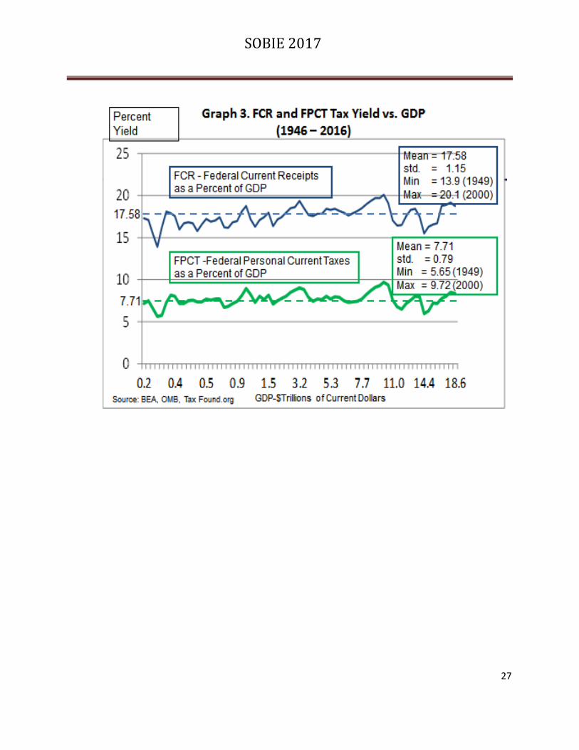
From graph 3, we observe that over time both federal personal current tax (FPCT) and
federal current receipts (FCR) exhibit stability of yield relative to GDP. In this graph, study
results are plotted and show that FPCT had a mean yield of 7.71% with a standard deviation of
0.79, while FCR had a mean yield of 17.58% with a standard deviation of 1.15 over the study
period. From graph 4, we see that as the yield of FPCT and FCR remains stable, GDP grew
dramatically from 227.8 $billion to 18.55 $trillion, while marginal tax rates declined from a high
of 92% in 1952 to a low of 28% in 1990 before ending at 39.6% at the end of the study period.
Over the study period, the correlation between GDP increases compared to the stepped decreases
in marginal tax rates was r = -0.815. From graph 5, we observe the growth in nominal tax
revenue for both FCR and FPCT. The average yield for both variables remains relatively stable.
We find it interesting that minimum and maximum yield occurred for both study variables in
1949 (min yield at a marginal rate of 91%) and in 2000 (max yield at a marginal rate of 39.6%)
respectively.
SOBIE 2017
27

SOBIE 2017
28

SOBIE 2017
29
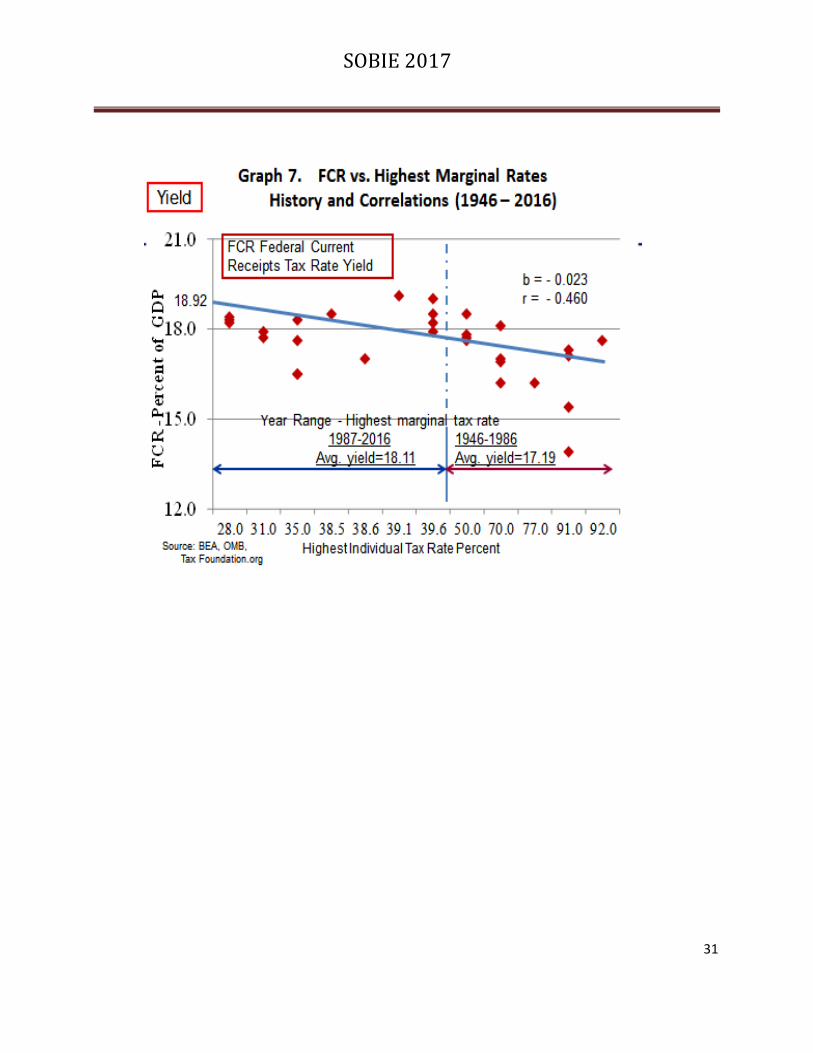
Correlation analysis between the applicable marginal tax rates by year and the yield for
both FPCT and FCR is reviewed in graphs 6 and 7. As previously shown in graph 3, both
variables have a small standard deviation relative to their stable means over the study period.
Both are negatively correlated with increasing marginal rates (FPCT with r = -0.21 and FCR with
r = -0.46). To further test this correlation over time, we divided the highest marginal rates into
two sets. For set one we defined the high rate years (1946-1986) as those with the highest
marginal rates from 50% to 92%. For set two we defined the low rate years (1987-2016) as
those with the highest marginal rates from 28% to 39.6%. Once again we saw an improved
average yield for both FPCT and FCR when comparing the results from defined high rate years
to those defined as low rate years. In the conclusions drawn from an earlier research work
focused on tax yield, Fielding and Cobb (2016) found that the average tax revenue as a percent
of GDP was consistently higher over the period of lower federal tax rates. Analytical results are
summarized in table 2.

SOBIE 2017
30
SOBIE 2017
31

SOBIE 2017
32
Conclusions
Laffer (2010) brought attention to the fact that taxpayers in the higher income brackets
are capable of tax decisions that can change their taxable income. In the same year, Houser
(2010) emphasized that entrepreneurship was discouraged by higher taxes. In both cases, these
researchers were referring to the effect higher tax rates have on the decisions individuals make
concerning income.
Our research accepts that tax yield stability exists over time and asks what variables play
a role in this fact. Beginning in the 1990s, Hauser and others began to review the available data
and observed those tax revenue patterns that seemed to question the strength of tax rates in the
revenue equation. From our data analysis, we can conclude that over the seventy years spanned
in this study, yield from federal personal current tax (FPCT) and from federal current receipts
(FCR) was stable, regardless of marginal rates. Though not statistically significant, slightly
higher average tax yields occurred during defined low tax rate years for both study variables.
This result, based on a large sample size, took place during a period when GDP generally rose
and highest marginal tax rates generally declined. The simple conclusion is that Tax Yield = Tax
Revenue/GDP. And, since both study variables are shown to have relatively constant yield over
time, increased tax revenue is best obtained from growth in GDP

SOBIE 2017
33
For future research, we feel that lag in revenue flow should be correlated with changing
tax rates. We should look for ways to track, quantify, and include subjective data, including the
consumer confidence index and the influence of job creation data. Any factor that may influence
the redirection or sheltering of income should also be considered.
References
Barro, R. J. (2009). Government Spending is No Free Lunch, The Wall Street
Journal, (Eastern Edition), 22 January, New York, NY, p. A17.
BEA (2016). NIPA tables. at http://www.bea.gov
Fielding W. T. and R. Cobb (2016). U.S. Marginal Tax Rate, GDP, and Income Taxes Paid
(1946-2016), JSU Economic Update, 78-82.
FRED (2016). Federal Receipts as Percent of Gross Domestic Product. Federal
Reserve Bank of St. Louis, retrieved from http://fred2/series/FYFRGDA188S
Hao Li On (2010). Correlation among income tax rate, tax receipts, and GDP,
International Business Times, 30 August, retrieved from http://ibtimes.com
Hauser, W. K. (2010, November 26). There’s No Escaping Hauser’s Law, The
Wall Street Journal, retrieved from http://www.wsj.con/articles/SB
Hauser, W. K. (1993, March 25). The Tax and Revenue Equation, The Wall Street
Journal, op-ed, retrieved from http://www.wsj.con/articles/SB
Hauser, W. K. (1996). Taxation and Economic Performance. Stanford, California:
Hoover Institution Press, 13-16.
Heritage Foundation (2016). Federal Budget in Pictures. The Heritage
Foundation, retrieved from http://heritage.org/federalbudget/embed
Laffer, A. (2010, August 2). The Soak-the-Rich Catch-22, The Wall Street
Journal, retrieved from http://www.wsj.con/articles/SB
OECD (2014). Total tax revenue, Taxation: Key Tables from the Organization for
Economic Co-operation and Development OECD, No. 2. retrieved from
http://dx.doi.org/10.1787/taxrev-table-2013-1-en
OMB (2016). Historical tables 3.2, at http://www.whitehouse.gov/omb/budget
Ranson, D. (2010, August 4). The Limit of Tax Revenues, National Center for
SOBIE 2017
34
Policy Analysis, Brief Analysis No. 716, retrieved from http://ncpa.org
Ranson, D. (2008, May 20). You Can’t Soak the Rich, The Wall Street,
Commentary, retrieved from http://www.wsj.con/articles/SB
Smith, A. (1776). An Inquiry into the Nature of Causes of the Wealth of Nations.
London: W. Strahan and T. Cadell Publishing.
Tax Foundation (2016). Federal Individual Income tax Rate History, retrieved from
http://taxfoundation.org
TPS (2017). Source of Revenue as Share of GDP, Tax Policy Center, retrieved
from http://taxpolicycenter.org/statistics/source
World Bank (2014). Tax revenue (% of GDP). World Bank, retrieved from
http://data.worldbank.org

SOBIE 2017
35
Financing Versus Other Input Costs: The Case of Iowa Agriculture
Producers
Robert Preston, Northern State University
John E. Peterson, Northern State University
Todd Muehler, Northern State University
Abstract
Borrowing is a function of convenience, relationships, and creditworthiness among other factors.
For those in the business of the production of agricultural products, the cost of borrowing for
their business is an input cost, similar to seeds, chemicals, fertilizers and fuel for the farm
vehicles. This study will examine agricultural producers with respect to the cost (distance
traveled) to obtain various agricultural inputs. What is unknown is whether the distance
traveled to obtain financing differs from that for obtaining seed, chemicals, fuel, and feed? This
study will examine Iowa ag producers as to whether they shop for financing differently from
other inputs. The results may provide insight into how ag producers view credit versus other
inputs.
Introduction
Agriculture producers are a mainstay of the local economies in which they operate. Their
support of the local economies is vital to the rural communities. The rural communities provide
support to the ag producers with those products and services on which the producers depend for
their business and farm families.
Studies have examined that relationship between the ag producer and the rural community, and
the relationship between lenders and loan performance when the distance between the lender and
the borrower increases. Foltz, Jackson-Smith and Chen (2002) studied the purchasing patterns of
large and small dairy farms. Gebremedhin and Christy (1996) studied the implications for small
farms resulting from structural changes in U.S Agriculture. Yeager (2004) studied the effects of
local economic shocks on the demise of community banks. DeYoung, Glennon and Nigro
(2006) studied the borrower-lender distance. Berger, Cowan and Frame (2010) studied the use
of credit scoring in small business lending by community banks and the attendant effects on
credit availability and profitability. Agarwal and Hauswald (2010) studied the relationship
between distance and private information in lending. A combination of the results of these
studies can inform the relationship between the lender and the small business ag producer found
predominately in the north central United States. To add a further dimension and to attempt to
view the lender/producer/community relationship from the perspective of the ag producer, this
study will examine Iowa ag producers as to whether they shop for financing differently from
other inputs. This study seeks to determine whether the distance traveled by the ag producer to

SOBIE 2017
36
obtain financing differs from that for obtaining seed, chemicals, fuel and feed, as inputs to farm
production.
According to Agarwal and Hauswald (2010), “Any borrower deemed creditworthy always
obtains credit from the closest bank and would never switch lenders.” Thus, creditworthy
farmers should always obtain credit, from the closest bank. If that bank is in the local
community where the farmer obtains other production inputs such as feed, seeds, fuel and
fertilizer and other chemicals, the distance from the farm to that source of input costs should be
insignificant. The local community may not have a provider of the needed input so the farmer
may need to go elsewhere for that input. If any of the inputs are not available in the local
community, or if the farmer choses to obtain the input from sources not in the local community,
then the farmer would need to travel a greater distance to obtain the needed input for production.
The farmer may desire a specific seed or feed or specific chemicals not available in the local
community. The farmer’s choice of most input elements may be based on cost or preference or
performance. With respect to the input cost of credit (interest), the choice of provider is also
influenced by the lender’s expertise and service and the borrower’s creditworthiness. Since
credit generally does not require physical transport to be delivered, once obtained, the additional
instances of need also may not involve any additional transportation cost to access, which
differentiates finance from most other inputs. This may result in a farmer viewing financing
differently than other farm production inputs.
Our main contribution to the literature is to provide this different perspective, that from the view
of the farmer, as to behavior, seeking inputs to production locally of from suppliers beyond the
local community, and whether the farmer differentiates between types of input, specifically the
input of finance cost, from those other farm inputs used in the operation.
DATA
To study the question of whether farmers shop for financing differently from other inputs we
examined the results of the U.S Department of Agriculture 2008 Agricultural Resource
Management Survey, Cost and Returns Report (USDA 2008 ARMS Phase III Survey) (the
“USDA survey”) to determine whether the distance traveled by the ag producer to obtain
financing differs from that for obtaining seed, chemicals, fuel and feed, as inputs to farm
production. The USDA survey data contains responses from farmers regarding where those
completing the survey buy the majority of input items used by the farming operation and lists:
fuel, fertilizer and chemicals, feed and seed, farm credit, household consumer goods, and
household durable goods. The survey asks those completing the survey to identify the distance
from the farm in miles, whether the purchase was made in the same county as the home or
operation/farm, and asks the those completing the survey to identify the main reason if not
purchased in the nearest town or city, giving a list of 6 reasons from which a selection can be
made (price of the input, not available, quality or performance, supplier services/information,
other support services, or other).
SOBIE 2017
37
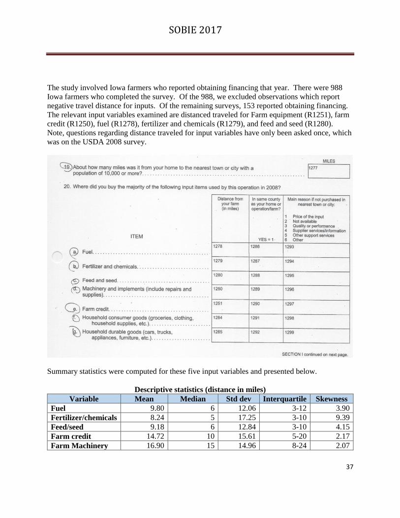
The study involved Iowa farmers who reported obtaining financing that year. There were 988
Iowa farmers who completed the survey. Of the 988, we excluded observations which report
negative travel distance for inputs. Of the remaining surveys, 153 reported obtaining financing.
The relevant input variables examined are distanced traveled for Farm equipment (R1251), farm
credit (R1250), fuel (R1278), fertilizer and chemicals (R1279), and feed and seed (R1280).
Note, questions regarding distance traveled for input variables have only been asked once, which
was on the USDA 2008 survey.
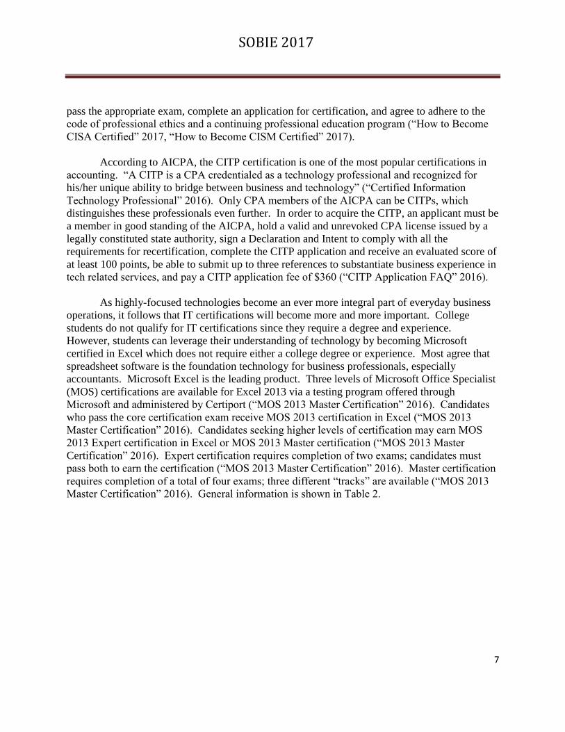
Summary statistics were computed for these five input variables and presented below.
Descriptive statistics (distance in miles)
Variable Mean Median Std dev Interquartile Skewness
Fuel 9.80 6 12.06 3-12 3.90
Fertilizer/chemicals 8.24 5 17.25 3-10 9.39
Feed/seed 9.18 6 12.84 3-10 4.15
Farm credit 14.72 10 15.61 5-20 2.17
Farm Machinery 16.90 15 14.96 8-24 2.07

SOBIE 2017
38
All inputs are highly skewed to the right. Given non-negative nature of distance this result is
expected.
These results appear consistent with expectations of the likely behavior of farm operators. As
measured by the medians set forth above, over half of the purchases of fuel, fertilizer/chemicals,
and feed/seed were made by the farmer within a distance of less than 6 miles from the farm site.
It would be expected that a farmer would buy fuel, fertilizer and feed in bulk and have those
delivered to the farm site. As a result, the location of the purchase may be more subject to
interpretation with some who consider the delivery to the farm site as the location of the
purchase and thus the distance traveled would be very small. Others may consider the purchase
location to be the office of the supplier, while still others may consider the purchase location to
be the location of the supplier’s representative or product staging location. It is unlikely that the
farm operator would leave the farm site, travel to the supplier, obtain the input variable (fuel,
fertilizer/chemicals or feed/seed) and physically transport those in any significant quantity back
to the farm site. In summary, what are thought of as traditional farm inputs --Fuel and
fertilizer/chemicals and feed/seed are locally provided. For example, there are multiple seed
dealers who also are farmers. On the other hand, farm credit is a regulated business.
The data suggests that farmers traveled the greatest distance from the farm site for farm
machinery/implements, including repairs and supplies. This is based on the median distance
traveled for machinery. Again, this is consistent with expectations. Farm machinery and
implements are infrequent purchases by farmers. Farm machinery and implements also have an
economy of scale. There is not a direct linear relationship between the equipment and the
number of acres planted. Rather, a step relationship occurs with the same equipment used for a
range of acres planted and efficiencies are realized as the same equipment is used to produce
more output and over more acres .While necessary for production inputs such as feed/seed,
fertilizer/chemicals and fuel, they are not themselves strictly input such as the raw materials and
production resources of a manufacturer. The allocation of the usage cost in terms of depreciation
is appropriate as an input cost, but that is an accounting entry not involving a third party
transactions such as the case with a purchase of machinery. Machinery/implements are also not
available in many communities surrounding farmers. Because of the infrequent nature of the
demand, machinery/implement dealers typically locate in a hub community serving many
community markets and thus the distance traveled by the farmer to the dealer would be expected
to be further than that to the local community, except for those few who are most nearly located
by the hub. In addition, as with the other bulk inputs of fuel, fertilizers/chemicals and feed/seed,
farmers take delivery of the machinery and often repairs are provided at the farm site, even if the
purchase was done at a distance and thereby may consider the distance to purchase the
machinery input to be negligible or near the farm site. To obtain machinery supplies the farmer
may need to travel to the dealer, because many manufacturers of farm machinery now limit
repairs or parts to only those provided from authorized manufacturer representatives, and the
supplies available in more nearby communities do not generally qualify as authorized.

SOBIE 2017
39
Farm credit is generally obtained at a distance further away from the farm site than those
providing fuel, fertilizer/chemicals and feed/seed, but closer than those providing farm
machinery/implements. Based on the median distance, more than half of the farmers obtained
credit from providers at a distance of more than 10 miles from the farm site which the traditional
inputs of fuel, fertilizer and feed was less than 6 miles and farm machinery was obtained at a
distance of more than 15 miles from the farm site. Although not considered part of this study
which was focused on the farm business input components, the distance traveled for farm credit
was consistent with that traveled by the farmers for consumer goods.
Unlike the other farm business input components, farm credit is unique in that it does not require
physical transportation to be “obtained” and utilized in the farming operation. Farmers, like
most borrowers, obtain credit by traveling to the provider location to arrange the granting of the
credit. The credit is then used in the farming operation by the farmer accessing that credit
through checks or draws processed by the provider which does not require additional travel for
that access. Unlike the bulk inputs of fuel, fertilizer and feed, the provider does not need to
transport the input of farm finance from the provider’s location to the farm site. Similar to the
acquisition of farm equipment, the farmer typically travel to the provider’s location for the initial
acquisition (although more often for the larger farmers, the provider of both machinery and
finance will come to the farm site for the acquisition), but unlike the equipment repairs and
supplies, the provider need not make additional trips to the farm site to continue providing that
farm credit input component.
Farmers and the providers of farm inputs are price sensitive and for the physical inputs of fuel,
fertilizer/chemicals, feed/seed and machinery the cost of transportation of that input is part of the
price calculation. For farm credit the transportation cost component is significantly less because
the transportation requirements are minimal. However, as noted above by Agarwal and
Hauswald (2010) “Any borrower deemed creditworthy always obtains credit from the closest
bank and would never switch lenders.” Thus, creditworthy farmers should always obtain credit,
from the closet bank. If that bank is in the local community where the farmer obtains other
production inputs such as feed, seeds, fuel and fertilizer and other chemicals, the distance from
the farm to that source of input costs should be insignificant. If the farmer travels beyond the
local community, the provider of farm credit will generally incur and adverse selection premium
passed on to the borrowing farmer in the form of a higher interest rate on the credit provided, due
to the higher risk of market and information uncertainty attributed to the greater distance
between the borrower and the lender.
The financial services market is highly regulated and not all local providers of credit may be able
to extend farm credit as required by the local farmer due to financial regulations. Farms continue
to expand in size and in borrowing requirements. Banks have been consolidating over the past
25 years and as they do many banks in rural communities are absorbed into other institutions.
This consolidation often allows the local office in the rural community to consider larger loan
requests than were possible before the consolidation, however, in many cases even with the
consolidation, the borrowing requirements exceed the authorized capacity of the local banking

SOBIE 2017
40
office. When this happens the borrower may find it necessary to seek credit from sources
beyond the local community. While this study does not have the type of data to allow specific
determination of individual farm credit requirements, the data seems to indicate that the farmers
tend to seek farm credit at distances from the farm that exceed those necessary for the bulk farm
inputs of fuel, fertilizer/chemicals and feed/seed.
The data of this study may provide some clarification, however. The data on farm input
components contain not only distance, but also seek the selection of a choice of 6 reasons if the
farmer-responder, to the survey did not buy the variable (input component) locally. If the farmer
did by locally, no response or a “0” response would be provided. If the farmer did not buy
locally because of the price of the variable, the response would be “1”. If the farmer did not buy
locally because of the variable was not available locally, the response would be “2”. If the
farmer did not buy locally because of the variable did not meet the quality or performance of the
farmer, the response would be “3”. If the farmer did not buy locally because of the supplier
services/information of the variable did not meet the requirements of the famer, the response
would be “4”. If the farmer did not buy locally because of other support services of the variable,
the response would be “5”. If the farmer did not buy locally because of the other factors of the
variable, the response would be “6”.
The following provide the distribution of the responses to the question on the survey regarding
the farmer-responder to the survey did not buy the variable (input component) locally.
Main reason farmer did NOT buy Fuel in nearest town or city
54.9% Bought Fuel at town or city nearest the farm (0)
14.4% Did not buy Fuel at nearest town or city because of price (1)
5.2% Did not buy Fuel at nearest town or city because it was not available (2)
3.3% Did not buy Fuel at nearest town or city because of quality or performance (3)
9.2% Did not buy Fuel at nearest town or city because of Supplier services/information
(4)
SOBIE 2017
41
21.3% Did not buy Fuel at nearest town or city because of Other support services (5)
11.8% Did not buy Fuel at nearest town or city because of Other reasons (6)
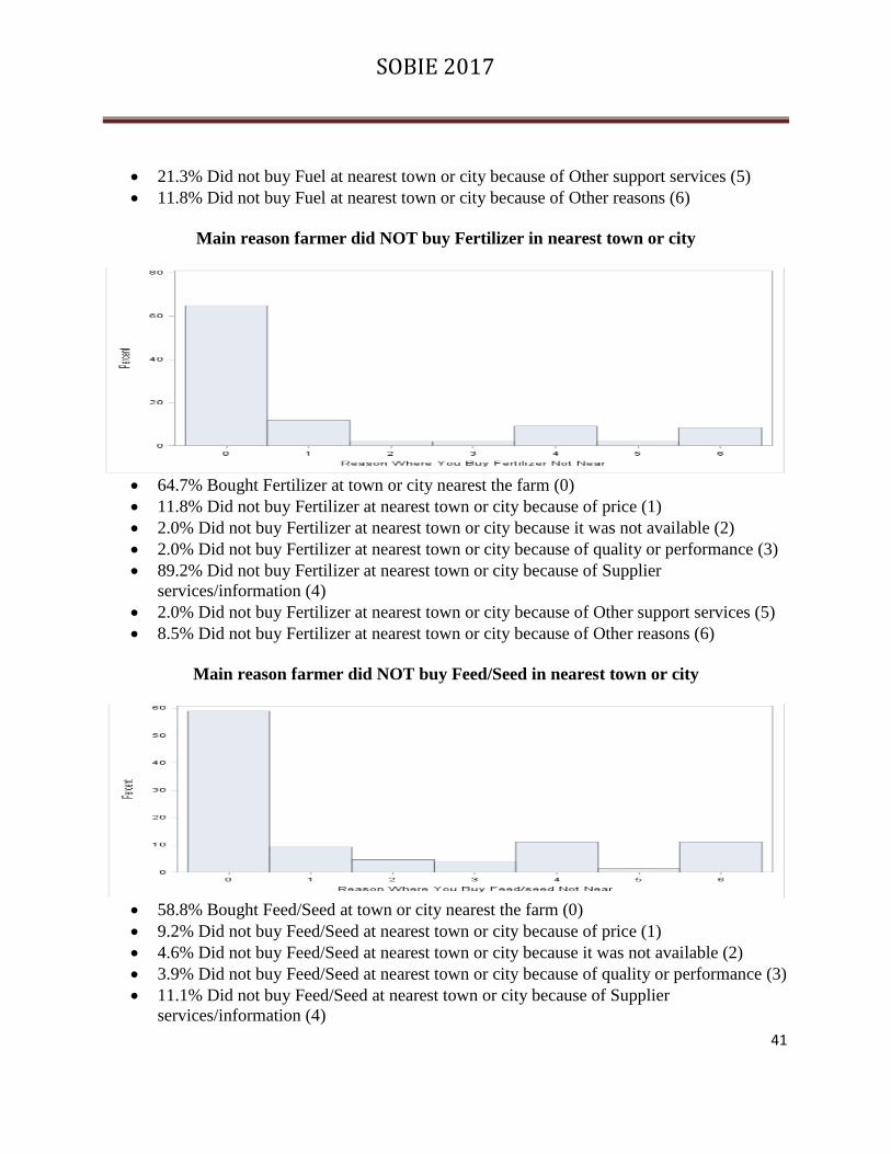
Main reason farmer did NOT buy Fertilizer in nearest town or city
64.7% Bought Fertilizer at town or city nearest the farm (0)
11.8% Did not buy Fertilizer at nearest town or city because of price (1)
2.0% Did not buy Fertilizer at nearest town or city because it was not available (2)
2.0% Did not buy Fertilizer at nearest town or city because of quality or performance (3)
89.2% Did not buy Fertilizer at nearest town or city because of Supplier
services/information (4)
2.0% Did not buy Fertilizer at nearest town or city because of Other support services (5)
8.5% Did not buy Fertilizer at nearest town or city because of Other reasons (6)
Main reason farmer did NOT buy Feed/Seed in nearest town or city
58.8% Bought Feed/Seed at town or city nearest the farm (0)
9.2% Did not buy Feed/Seed at nearest town or city because of price (1)
4.6% Did not buy Feed/Seed at nearest town or city because it was not available (2)
3.9% Did not buy Feed/Seed at nearest town or city because of quality or performance (3)
11.1% Did not buy Feed/Seed at nearest town or city because of Supplier
services/information (4)
SOBIE 2017
42
1.3% Did not buy Feed/Seed at nearest town or city because of Other support services (5)
11.1% Did not buy Feed/Seed at nearest town or city because of Other reasons (6)
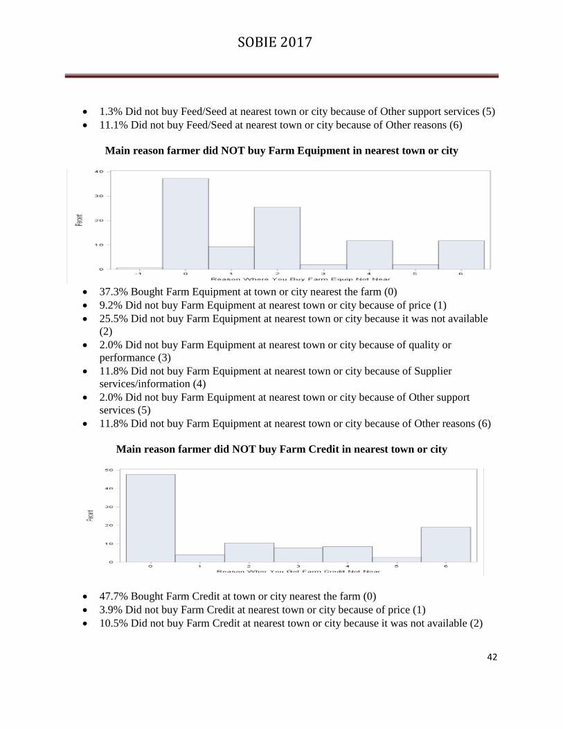
Main reason farmer did NOT buy Farm Equipment in nearest town or city
37.3% Bought Farm Equipment at town or city nearest the farm (0)
9.2% Did not buy Farm Equipment at nearest town or city because of price (1)
25.5% Did not buy Farm Equipment at nearest town or city because it was not available
(2)
2.0% Did not buy Farm Equipment at nearest town or city because of quality or
performance (3)
11.8% Did not buy Farm Equipment at nearest town or city because of Supplier
services/information (4)
2.0% Did not buy Farm Equipment at nearest town or city because of Other support
services (5)
11.8% Did not buy Farm Equipment at nearest town or city because of Other reasons (6)
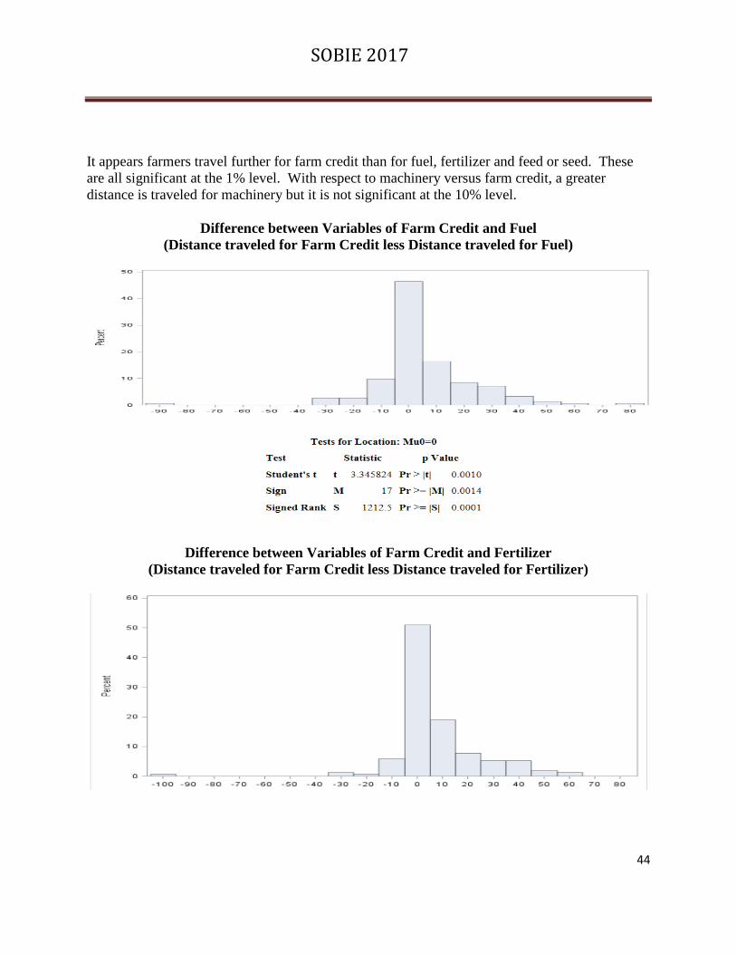
Main reason farmer did NOT buy Farm Credit in nearest town or city
47.7% Bought Farm Credit at town or city nearest the farm (0)
3.9% Did not buy Farm Credit at nearest town or city because of price (1)
10.5% Did not buy Farm Credit at nearest town or city because it was not available (2)

SOBIE 2017
43
7.8% Did not buy Farm Credit at nearest town or city because of quality or performance
(3)
8.5% Did not buy Farm Credit at nearest town or city because of Supplier
services/information (4)
2.6% Did not buy Farm Credit at nearest town or city because of Other support services
(5)
19.0% Did not buy Farm Credit at nearest town or city because of Other reasons (6)
METHODOLOGY & ANALYSIS
To assess if there is a significant difference between how a farmer views farm credit and the
willingness to travel a difference distance to obtain that farm production input variable compared
the distance traveled for financing versus other farm inputs. For each farmer, we calculate the
difference in distance traveled for financing minus other input. Therefore, the null hypothesis of
no difference in distance traveled would be:
H0 : μd = 0 H1 : μd ≠ 0
Both parametric (paired t-test) and nonparametric (Sign test and Signed Rank test) test statistics
were used for the comparison. We compared the results of the distance travel for:
Farm credit versus Fuel
Farm credit and Fertilizer
Farm credit and Feed/Seed
Farm credit and Machinery and implements (including repairs and supplies)
Farm machinery and Fuel
Farm machinery and Fertilizer
Farm machinery and Feed/Seed
Fuel and Fertilizer
Fuel and Feed/Seed
Fertilizer and Feed/Seed
The summary results are presented below. Differences, X1i-X2i, where X1 is farm credit and X2
is the other farm input were computed.
Differences Farm Credit – other farm input variable
Variable Mean T Sign Signed Rank
Farm credit – Fuel 4.915 3.35*** 17*** 1212.5***
Farm credit – Fertilizer 6.48 4.63*** 23*** 1660***
Farm-credit – Feed 5.54 3.73*** 19.5*** 1291.5***
Farm credit - Machinery -2.189 -1.35 -9 -594.5
***, **,* denotes statistical significance at 1%, 5% and 10% level
SOBIE 2017
44
It appears farmers travel further for farm credit than for fuel, fertilizer and feed or seed. These
are all significant at the 1% level. With respect to machinery versus farm credit, a greater
distance is traveled for machinery but it is not significant at the 10% level.
Difference between Variables of Farm Credit and Fuel
(Distance traveled for Farm Credit less Distance traveled for Fuel)
Difference between Variables of Farm Credit and Fertilizer
(Distance traveled for Farm Credit less Distance traveled for Fertilizer)
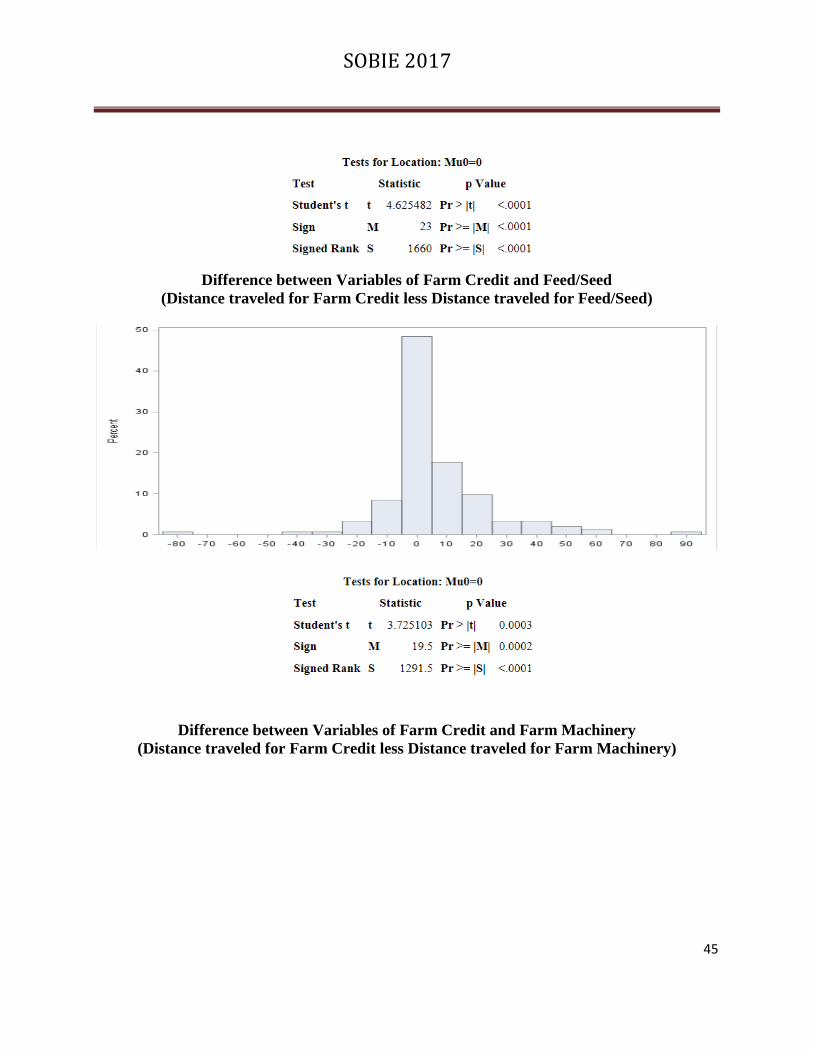
SOBIE 2017
45
Difference between Variables of Farm Credit and Feed/Seed
(Distance traveled for Farm Credit less Distance traveled for Feed/Seed)
Difference between Variables of Farm Credit and Farm Machinery
(Distance traveled for Farm Credit less Distance traveled for Farm Machinery)

SOBIE 2017
46
Difference between Variables of Farm Machinery and Fuel
(Distance traveled for Farm Machinery less Distance traveled for Fuel)
Difference between Variables of Farm Machinery and Fertilizer
(Distance traveled for Farm Machinery less Distance traveled for Fertilizer)

SOBIE 2017
47
Difference between Variables of Farm Machinery and Feed/Seed
(Distance traveled for Farm Machinery less Distance traveled for Feed/Seed)
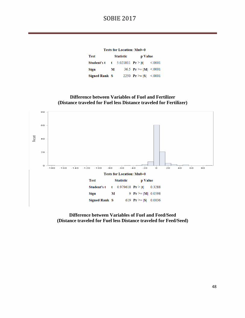
SOBIE 2017
48
Difference between Variables of Fuel and Fertilizer
(Distance traveled for Fuel less Distance traveled for Fertilizer)
Difference between Variables of Fuel and Feed/Seed
(Distance traveled for Fuel less Distance traveled for Feed/Seed)
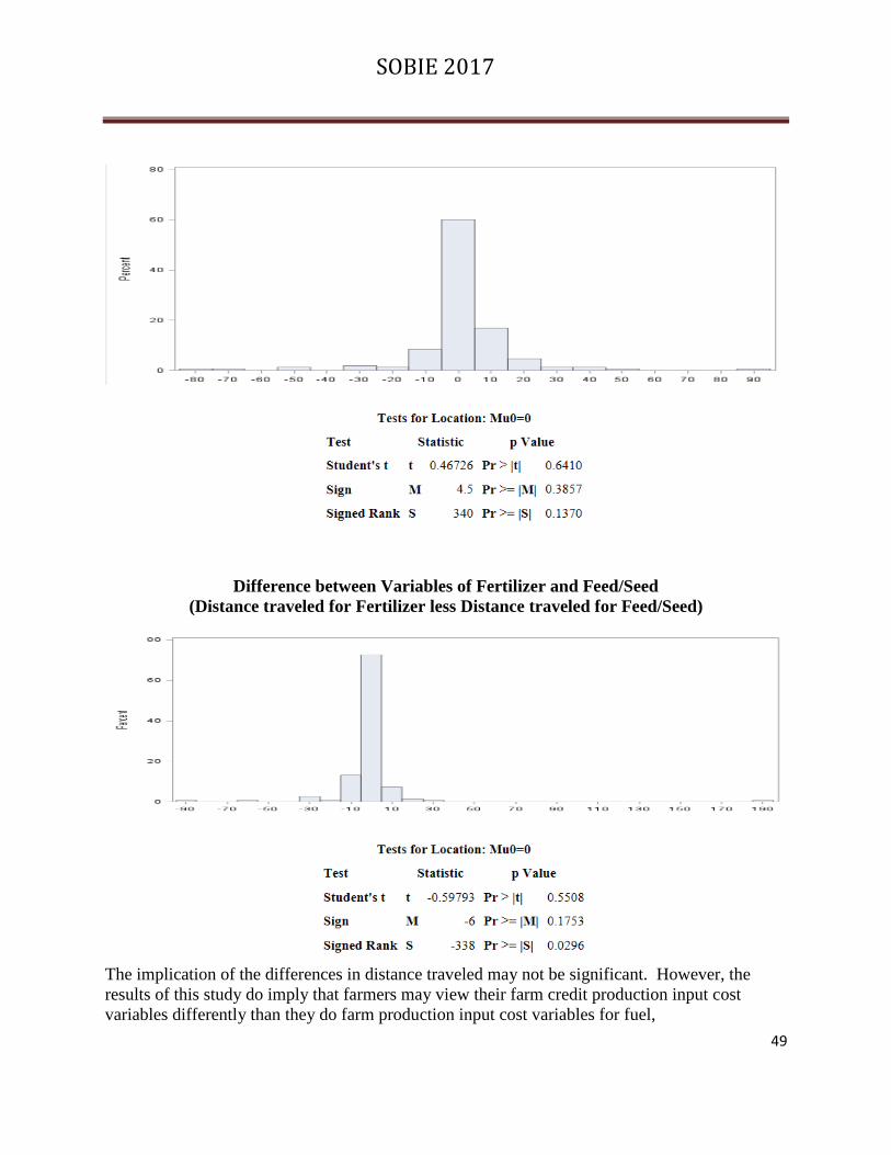
SOBIE 2017
49
Difference between Variables of Fertilizer and Feed/Seed
(Distance traveled for Fertilizer less Distance traveled for Feed/Seed)
The implication of the differences in distance traveled may not be significant. However, the
results of this study do imply that farmers may view their farm credit production input cost
variables differently than they do farm production input cost variables for fuel,
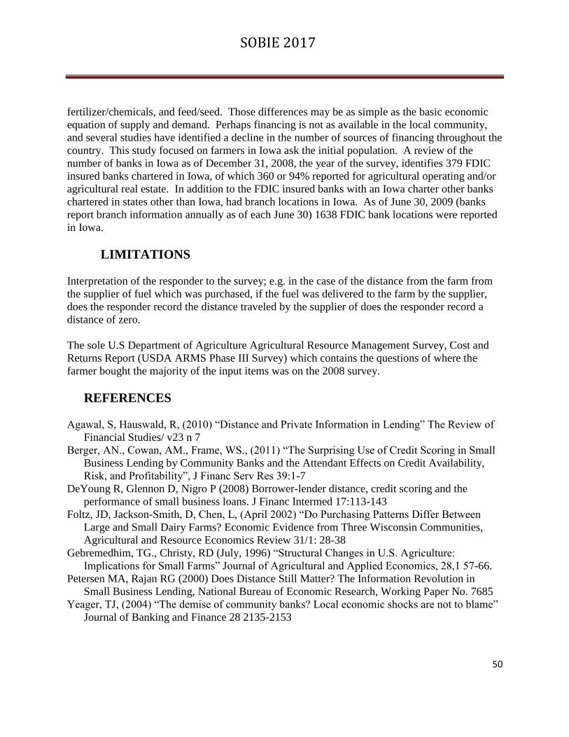
SOBIE 2017
50
fertilizer/chemicals, and feed/seed. Those differences may be as simple as the basic economic
equation of supply and demand. Perhaps financing is not as available in the local community,
and several studies have identified a decline in the number of sources of financing throughout the
country. This study focused on farmers in Iowa ask the initial population. A review of the
number of banks in Iowa as of December 31, 2008, the year of the survey, identifies 379 FDIC
insured banks chartered in Iowa, of which 360 or 94% reported for agricultural operating and/or
agricultural real estate. In addition to the FDIC insured banks with an Iowa charter other banks
chartered in states other than Iowa, had branch locations in Iowa. As of June 30, 2009 (banks
report branch information annually as of each June 30) 1638 FDIC bank locations were reported
in Iowa.
LIMITATIONS
Interpretation of the responder to the survey; e.g. in the case of the distance from the farm from
the supplier of fuel which was purchased, if the fuel was delivered to the farm by the supplier,
does the responder record the distance traveled by the supplier of does the responder record a
distance of zero.
The sole U.S Department of Agriculture Agricultural Resource Management Survey, Cost and
Returns Report (USDA ARMS Phase III Survey) which contains the questions of where the
farmer bought the majority of the input items was on the 2008 survey.
REFERENCES
Agawal, S, Hauswald, R, (2010) “Distance and Private Information in Lending” The Review of
Financial Studies/ v23 n 7
Berger, AN., Cowan, AM., Frame, WS., (2011) “The Surprising Use of Credit Scoring in Small
Business Lending by Community Banks and the Attendant Effects on Credit Availability,
Risk, and Profitability”, J Financ Serv Res 39:1-7
DeYoung R, Glennon D, Nigro P (2008) Borrower-lender distance, credit scoring and the
performance of small business loans. J Financ Intermed 17:113-143
Foltz, JD, Jackson-Smith, D, Chen, L, (April 2002) “Do Purchasing Patterns Differ Between
Large and Small Dairy Farms? Economic Evidence from Three Wisconsin Communities,
Agricultural and Resource Economics Review 31/1: 28-38
Gebremedhim, TG., Christy, RD (July, 1996) “Structural Changes in U.S. Agriculture:
Implications for Small Farms” Journal of Agricultural and Applied Economics, 28,1 57-66.
Petersen MA, Rajan RG (2000) Does Distance Still Matter? The Information Revolution in
Small Business Lending, National Bureau of Economic Research, Working Paper No. 7685
Yeager, TJ, (2004) “The demise of community banks? Local economic shocks are not to blame”
Journal of Banking and Finance 28 2135-2153
SOBIE 2017
51
Are College Football Betting Markets Efficient? Evidence from
Interconference Play
Evan Moore, Auburn University at Montgomery
James Francisco, Auburn University at Montgomery
Abstract
This article tests the efficient market hypothesis (EMH) and the profitability of a simple
betting strategy in NCAA college football. We examine all games that have a point spread,
from September 2003 through January 2016, for inter-conference matches involving a
Power Five/Automatic Qualifying (P5/AQ) team. The tests reject the EMH for these
matchups, with a large subset of matches driving this result. The betting strategy evidence
suggests it is nonrandom but it is not profitable.
I. Introduction
Over $90 billion is bet on college and professional football (both legally and illegally) in
the United States annually (American Gaming Association, 2016). In 2014 alone, more
than 12 million individual bets were made on college football at the top offshore betting
sites (Fuhrman, 2015). With large amounts of money, and large numbers of individual
bettors, one might expect the market to trend toward efficiency. The Efficient Market
Hypothesis (EMH) states that asset prices reflect all publicly available information
(Mankiw, 2015). In this paper, we use a variety of existing tests within the literature to
ascertain if college football betting markets exhibit efficiency.
The most common form of college football wagering is betting on “spreads” or “lines”
which act as handicaps, and purport to reflect market perceptions about disparate team
quality, as well as other circumstances that could influence the outcome of a game (such
as home field advantage). Betting lines are listed as negative numbers for the favorite,
and positive numbers for the underdog. For example, if a sportsbook lists Team A “-7” vs
Team B, that means that in order to win the bet, Team A must defeat Team B by more
than 7 points in order for Team A’s bettors to “cover” (win the bet). Conversely, the
sportsbook would list Team B as “+7,” meaning 7 points would be added to Team B’s
score in order to determine who won the bet. If Team B achieves any outcome better than
a 7 point loss, Team B’s bettors have “covered.” If Team A defeats Team B by exactly 7
points, then the result for bettors is a tie, called a “push.”
Typically, spread betting on college football games in the United States have U.S. odds
of -110, which means that for every $110 a bettor wagers, he stands to win$ 100 for a

SOBIE 2017
52
cover, in addition to receiving his initial $110 back. If a bettor loses his wager, he loses
the entirety of the $110. In the case of a push, all bettors would be refunded their $110.
The remaining $10 is called the “vig” or “juice,” and goes to the sportsbook that offers
the wager. The spread, or line, adjusts over the course of the week leading up to the
game. Line movement functions as a price, with an increase in the line serving to make
the favorite more “expensive,” and the underdog “cheaper,” and vice versa. Because the
sportsbook can generate earnings via the “vig,” they often (though not always) attempt to
balance the amount of wagering on both sides in order to minimize exposure to any
particular outcome, and to take profit from the vig. Because of the existence of the vig, a
bettor adhering to the Kelly criterion would lose money if he merely covered half his
bets, and failed to cover half. In order to profit, a bettor would need to win in excess of
52.4% of his bets, at odds of -110.
II. Literature Review
Gandar, et al (1988) examined the efficiency of sports wagering by testing whether the
betting line generates a “fair bet.” The authors defined a “fair bet” in the context of
football wagering as one in which generates a .5 probability of covering for both the
favorite and the underdog. Equating fairness with efficiency, the authors tested efficiency
by jointly testing the intercept and slope coefficients in the following equation:
(1)𝑃𝑆1 = 𝛽0 + 𝛽1𝑉𝐿𝑖 + 𝑢𝑖 ,
where PS = the actual point spread, and VL = the Vegas line. The authors tested the joint
hypothesis of “fairness” that 𝛽0 =0, and 𝛽1 = 1 (Gandar et al 1988), asserting that such a
condition would indicated no profit as a result of the wagering.
Even and Noble (1992) expanded on the measures of fairness and market efficiency in
NFL wagering. Using both the OLS methods employed by Gandar et al (1988), as well as
a likelihood ratio test, the authors were generally unable to reject the null hypothesis of
fairness/efficiency across NFL betting on both spreads, and totals (the combined score of
both teams; bettors can wager on whether the combined total is “over” or “under” the
total). However, the authors also concluded that “fairness,” as such, is neither necessary
nor sufficient to sports wagering matchups.
Badrinathi and Kochman (1996) look beyond “fairness,” and searching merely for non-
random deviations from a probability of .5. Instead, they expand the inquiry to
“profitability,” testing whether any of three wagering “strategies” can be said to
consistently earn a profit (cover more than 52.38% of the time, assuming equal amounts
wagered, and odds of -110). The authors were able to find at least weak evidence of both
non-randomness and profitability for some strategies (Badrinathi and Kochman 1996).

SOBIE 2017
53
Paul and Weinbach (2005) adapted the Even and Noble (1992) log likelihood approach to
test not only for efficiency/non-randomness, but also for profitability. To test for
profitability, they adjusted the relevant probability of victory, from .5 to .524 (the number
needed to exceed the break-even point under the conditions outlined above). Using data
on totals wagering from college and Arena football, Paul and Weinbach (2005) found that
some naïve strategies (e.g. betting the under in every game, or every game in which the
wagering total exceeded some particular benchmark) produced results that were indeed
both non-random and profitable.
III. Data and Methodology
In this paper, we analyze wagering on spreads in college football games from the 2003-
2016 seasons. The data, acquired from the analytics firm Sports Insights, include the
opening and closing betting lines, and actual results, of every Division I college football
game over that period. College football teams are sorted into conferences, or miniature
“leagues” within the broader league of the NCAA. Division I is the division for the
largest, most competitive (and typically most well-funded) athletic programs.
For football only, the NCAA further subdivides Division into the Football Bowl
Subdivision (FBS), and the Football Championship Subdivision (FCS). The names reflect
the fact that the NCAA conducts a Championship for FCS, while it does not for FBS (the
only sport that the NCAA sponsors for which it does not conduct a championship). While
FBS teams tend to generate substantially more revenue than their FCS counterparts, they
are also required to invest more. FBS teams are required to play in stadia that have
capacity for at least 15,000 fans. FCS teams are limited to a maximum of 63 football
scholarships, and some FCS schools (and indeed some whole FCS conferences) do not
offer football scholarships. FBS schools, by contrast, may issue a maximum of 85
football scholarships, and must at a minimum offer 90% of that total on average over a
period of 2 years. As a result, FBS teams have many structural advantages over FCS
teams, and are typically expected to be much stronger.
Within the FBS, the conferences are further subdivided into 2 major groups: the Power
Five and the Group of Five. The Power Five conferences are the Southeastern Conference
(SEC), Atlantic Coast Conference (ACC), the Big Ten, the Big Twelve, and the Pacific
12 (PAC 12). Prior to 2014, a sixth conference, the Big East, was included with the
Power 5 in the group of Automatic Qualifying (AQ) conferences, or those conferences
whose champions automatically earned a spot in Bowl Championship (BCS) bowls. In
addition to stronger traditions (teams currently in AQ conferences have won the national
championship in each of the last 28 years), the AQ schools have structural advantages,
such as larger budgets, and the ability to offer “full cost of living” scholarships. As a
result, schools in AQ conferences are considered to be substantially stronger than FBS

SOBIE 2017
54
schools in non-AQ conferences; an even wider gap is perceived to exist between AQ
schools and FCS schools.
We apply the aforementioned non-randomness and profitability tests to the naïve strategy
of betting on AQ schools to cover against non-AQ and FBS schools. From the Sports
insight data set, we include all games featuring an inter-conference matchups involving
AQ teams for which there is a closing betting line. The overwhelming majority of games
featuring no line are matchups between AQ teams and FCS teams prior to 2007. Because
those matchups were generally anticipated to be lopsided affairs, most sportsbooks did
not offer lines on AQ-FCS matchups. However, in 2007, Appalachian State, then an FCS
team, upset Michigan in Michigan’s home stadium. Michigan was ranked #5 in the FBS
at that time, and had been a 3 point loss to Ohio State away from playing for the FBS
national championship the previous year. Subsequently, lines in AQ-FCS matchups
became more common. Now, having lines in such matchups is the norm. Note that
having “no line” refers to the absence of a line (and thus the absence of spread betting) at
all. If sportsbooks offer a contest as a “pick ‘em,” which is a line of “zero,” that simply
means that the straight up winner covers the spread bet. Such matchups are included in
the analysis here.
The data set includes 10,265 games, of which 1,983 are inter-conference matchups
involving one AQ team playing a non- AQ opponent. These 1,983 matchups are therefore
used in our study.
In addition to applying the methodology of Gandar et al (1988), shown in Equation (1),
we also utilize the log likelihood efficiency test employed by Even and Noble (1992), as
shown below:
(2) 𝐿𝑢 = 𝑛[𝑙𝑛( 𝑞^ )] + (𝑁 − 𝑛)𝑙𝑛(1 − 𝑞^), where n is number of covers, N is
number of matchups, and qˆ is ratio of covers to matchups.
Because this method assumes that an efficient market means that q=.5, we substitute .5
for 𝑞^, which yields the following likelihood ratio for the null hypothesis:
(3) 2(𝐿𝑢 − 𝐿𝑟) = 2{𝑛[𝑙𝑛( 𝑞ˆ ) − 𝑙𝑛(0.5)] + (𝑁 − 𝑛)[𝑙𝑛(1 − 𝑞ˆ ) − 𝑙𝑛(0.5)]}
We also utilized the Badarinathi and Kochman (1996) test for non-randomness, as shown
below:
(4) 𝑍1 = [𝑊 − 0.5(𝐵)] 𝑥 [𝐵(𝑝)(1 − 𝑝)] − 1/2,
where W is number of covers, B is the number of matchups, and p is probability of
winning, i.e. 0.5.
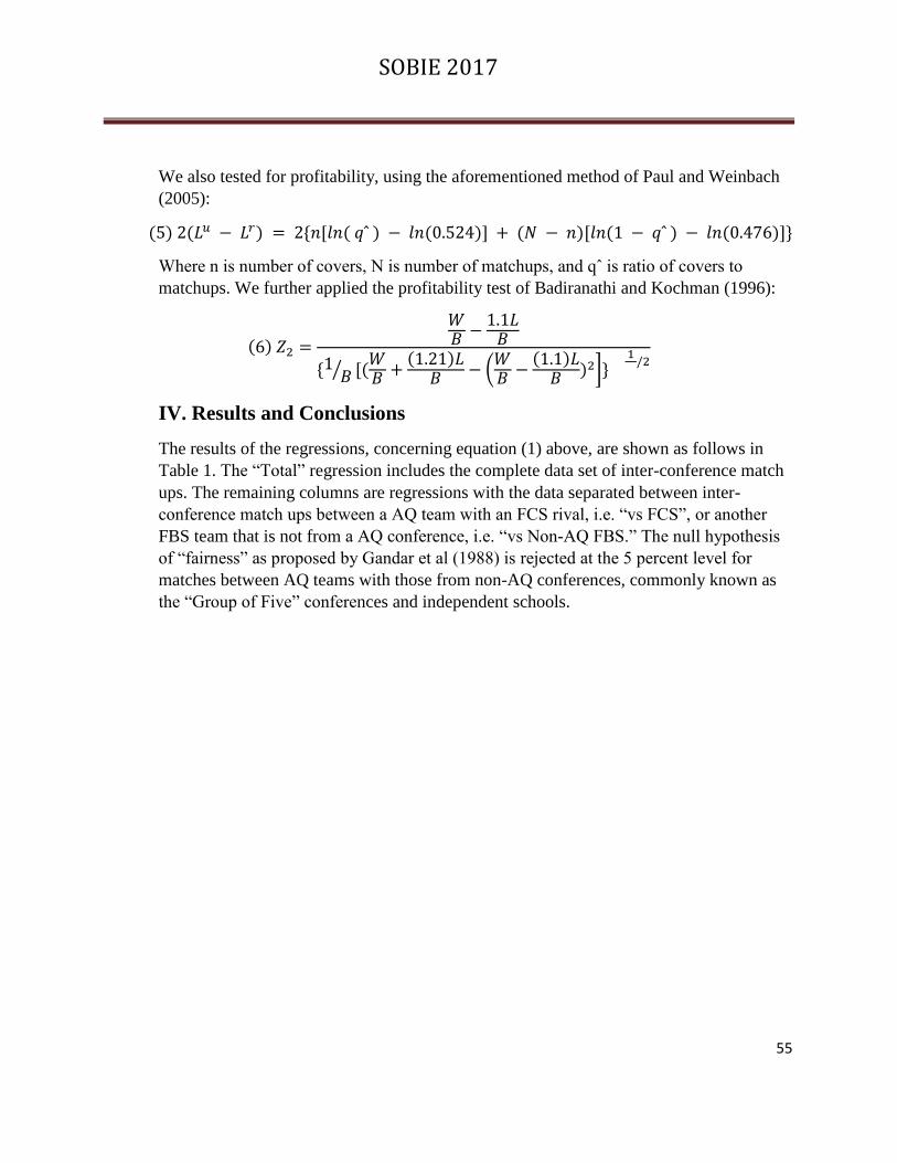
SOBIE 2017
55
We also tested for profitability, using the aforementioned method of Paul and Weinbach
(2005):
(5) 2(𝐿𝑢 − 𝐿𝑟) = 2{𝑛[𝑙𝑛( 𝑞ˆ ) − 𝑙𝑛(0.524)] + (𝑁 − 𝑛)[𝑙𝑛(1 − 𝑞ˆ ) − 𝑙𝑛(0.476)]}
Where n is number of covers, N is number of matchups, and qˆ is ratio of covers to
matchups. We further applied the profitability test of Badiranathi and Kochman (1996):
(6) 𝑍2 =
𝑊𝐵 −
1.1𝐿𝐵
{1𝐵⁄ [(
𝑊𝐵 +
(1.21)𝐿𝐵 − (
𝑊𝐵 −
(1.1)𝐿𝐵 )2]}
1/2
IV. Results and Conclusions
The results of the regressions, concerning equation (1) above, are shown as follows in
Table 1. The “Total” regression includes the complete data set of inter-conference match
ups. The remaining columns are regressions with the data separated between inter-
conference match ups between a AQ team with an FCS rival, i.e. “vs FCS”, or another
FBS team that is not from a AQ conference, i.e. “vs Non-AQ FBS.” The null hypothesis
of “fairness” as proposed by Gandar et al (1988) is rejected at the 5 percent level for
matches between AQ teams with those from non-AQ conferences, commonly known as
the “Group of Five” conferences and independent schools.

SOBIE 2017
56
Table 1. Regression results for the efficiency of point spreads Total
vs FCS
vs Non-AQ FBS
Coeff. St. dev Coeff St. dev. Coeff. St. dev.
Constant 0.148 0.446 2.386 2.272 0.274 0.452
Point Spread 1.032*** 0.019 0.934*** 0.065 1.057*** 0.022
N 1983
376
1607
F test 3000.0
3
205.71
2222.12
Point Spread = 1 Total
vs FCS
vs Non-AQ FBS
t test 2.90*
1.02
6.43**
p-value 0.089
0.312
0.011
Joint test of null hypothesis that the coefficients of Constant = 0 and Point spread = 1. Total
vs FCS
vs Non-AQ FBS
F test 1.99
0.55
3.73**
p-value 0.138
0.57
5
0.024
Notes: * indicates significance at the 10% level; ** indicates significance at the 5% level; *** indicates significance at the 1%
level.

SOBIE 2017
57
Table 2. AQ inter-conference matchups
Total vs FCS vs Non-AQ FBS
Games 1983 376 1607
Covers 1031 184 847
Not covered 931 185 746
Push 21 7 14
Percent cover 51.992 48.936 52.707
log like – fair bet 3.148* 0.170 4.712**
log like - profit 0.120 1.785 0.069
Z1 Nonrandom 1.774* -0.413 2.170**
Z2 Profitability 0.149 -0.967 0.631
Notes: The log-likelihood test statistics have a chi-squared distribution with one degree of freedom. The Z test statistics
have a normal distribution. * indicates significance at the 10% level and ** indicates significance at the 5% level.

SOBIE 2017
58
Results of the log likelihood and Z testing are presented in Table 2. The results indicate that the
simple betting strategy of the AQ team covering against an inter-conference rival is not
profitable at generally recognized levels of statistical significance. However, our results suggest
that the market is inefficient. Log likelihood testing of a fair bet is rejected at the 10 percent level
and Z testing at the 5 percent level. The results are further broken down into matchups of teams
from AQ conferences versus FBS non- AQ conferences, and versus FCS teams. This analysis
indicates that the non-randomness is driven by games between AQ schools and FBS schools
from non- AQ conferences, i.e. the “Group of Five” and independent schools, with log likelihood
and Z test results rejecting efficiency at the 5 percent level.
SOBIE 2017
59
References
Badarinathi, R. and Weinbach, A.P. (2005). “Bettor Preferences and Market Efficiency in
Football Totals Markets.” Journal of Economics and Finance (29)3. 409-415.
Even, W. E. and Noble, Nicholas R. (1992). “Testing Efficiency in Gambling Markets.” Applied
Economics, 24. 85-88.
Fuhrman, Todd. (2015, February 18). “Most Bet on College Football.” Retrieved from
http://www.outkickthecoverage.com/most-bet-on-college-football-games-021815
“Football Bets to Top $90 Billion for Second Straight Year.” (2016, September 7). Retrieved
from https://www.americangaming.org/newsroom/press-releasess/football-bets-top-90-billion-
second-straight-season
Gandar, J., Zuber, R., O’Brien, T., and Russo, B. (1988). “Testing Rationality in the Point
Spread Betting Market.” Journal of Finance, (43). 995-1007.
Mankiw, N. G. (2015). Principles of Economics. Stamford, CT. Cengage Learning.
Paul, R. J., and Weinbach, A.P. (2005). “Bettor Preferenes and Market Efficiency in Football
Totals Markets.” Journal of Economics and Finance, 29(3). 409-415.

SOBIE 2017
60
Teaching Students the Financial Statement Impact of the New Lease
Standard
Amanda Paul, Troy University
Richard Turpin, Troy University
Steve Grice, Troy University
Abstract
Accounting students cannot always appreciate why a lessee would prefer to keep a leased
asset and the related liability off of its balance sheet. Their lack of appreciation is sometimes
because they have not seen a simple comparison of two sets of financial statements – one set
keeps the asset/liability off of the lessee’s balance sheet while the other includes the
asset/liability on the lessee’s balance sheet.
Introduction
Currently, students are taught that lessees classify a lease as either operating or capital.
Intermediate accounting texts often tell students that a lessee has a desire to classify a lease as
operating instead of capital. The texts state that compared to an operating lease, a capital lease
has negative effects on a company’s debt-to-equity ratio. Although the texts’ statement is true, it
is rarely accompanied by an example that supports the statement in a way that most intermediate
accounting students can easily comprehend.
In February 2016, the FASB issued ASU 2016-02, Leases (Topic 842). The ASU
becomes effective for public entities for periods beginning after December 15, 2018, i.e.,
calendar years ending December 31, 2019. Under the new provision, a lessee will report a right-
of-use asset and a liability for all leases with the exception of those leases with a term of 12
months or less.
The purpose of this paper is to present, from a lessee’s perspective, an example that
compares current and future GAAP for leases and illustrates the impact the change will have on a
company’s financial statements and debt-to-equity ratio.
The Basics of Current Lease Accounting – Lessee Perspective
Under current GAAP, a lessee classifies a lease contract as either capital or operating. To
be classified as capital, the lease must be noncancelable and must meet at least one of the
following criteria:
1. The lease transfers ownership of the property to the lessee.
2. The lease contains a bargain purchase option.
SOBIE 2017
61
3. The lease term is equal to 75% or more of the estimated life of the leased asset.
4. The present value of the lessee’s minimum lease payments (excluding executor costs)
equals or exceeds 90% of the fair value of the leased asset.
For a lease that is classified as capital, a lessee records an asset and a liability at the
inception of the lease contract. The recorded asset and liability amounts are based on the present
value of the future lease payments. During the term of the lease, the lessee depreciates the
recorded asset. In addition, each lease payment is accounted for as both interest expense and as a
reduction of the recorded liability. For a lease that is classified as operating, a lessee simply
records periodic rental costs based on the current period’s lease payments.
The Basics Of Future Lease Accounting – Lessee Perspective
Under future GAAP, a lessee will classify all long-term, i.e., more than 12 months, leases
as either financing or operating. A long-term lease that meets the same general criteria as current
GAAP will be classified as financing. A long-term lease that does not meet these criteria will be
classified as operating. Under both classifications, a lessee will record a right-of-use asset and a
liability at the inception of the lease contract.
During the lease term, there will be differences in accounting for financing and operating
leases. Accounting for a financing lease will be the same as current accounting for a capital
lease, i.e., recognition of interest and depreciation expenses. Accounting for an operating lease
will result in a straight-line recognition of lease expense.
Example
The following presents an example that allows students to compare the financial
statement results of recording the same lease under current and future GAAP. The example also
shows students how to record the lease-related transactions. The example is broken into five
areas:
1. Students are given a simple balance sheet for a hypothetical company before the
company enters into a lease agreement as well as some other pertinent data.
2. Students are given the terms and conditions of a lease agreement.
3. Students are given the journal entries and resulting financial statements assuming the
lease is accounted for under current GAAP.
4. Students are given the journal entries and resulting financial statements assuming the
same lease is accounted for under future GAAP.
5. Students are given a comparison of the difference in selected financial statement ratios as
a result of the GAAP rules.
The primary purpose of the example is to allow students to compare how classifying a lease
under current GAAP versus future GAAP impacts a company’s debt-to-equity ratio. In addition,
the example helps students understand how to make various journal entries.

SOBIE 2017
62
Hypothetical Balance Sheet And Other Data
The Jones Service Company was incorporated on January 1, year 01. Immediately after
its incorporation, Jones’ balance sheet consisted of the following:
Cash $1,000,000
TOTAL ASSETS $1,000,000
Long-term debt $ 400,000
Common stock and additional paid-in-capital 600,000
TOTAL LIABILITIES AND STOCKHOLDERS’ EQUITY $1,000,000
Other pertinent year 01 data for Jones follow:
Jones’ incremental borrowing rate was 5%.
Jones did not declare any dividends or pay back any of its long-term debt.
Jones’ net income amounts for years 01, 02, and 03 were $900,000, $1,000,000, and
$1,200,000, respectively.
All of Jones’ annual revenue and expense amounts were equal to Jones’ annual receipt
and disbursement amounts.
Lease Agreement
Jones leased a piece of equipment from Smith Leasing Company by signing a lease
agreement dated January 2, year 01. The terms and conditions of the lease agreement as well as
other pertinent data follow:
The lease is noncancelable.
The lease term is three years; the equipment has a remaining useful life of ten years.
The lease requires Jones to make three annual lease payments of $100,000 with the first
lease payment on January 2, year 01.
Lease Accounting

SOBIE 2017
63
Current GAAP – Assuming the lease agreement did not meet any of the criteria for
classification as a capital lease, Jones accounted for the lease as an operating lease and recorded
the following lease-related entries during years 01, 02, and 03:
01 02 03
Lease expense $100,000 $100,000 $100,000
Cash $100,000 $100,000 $100,000
Future GAAP – Assuming the lease agreement did not meet any of the criteria for
classification as a financing lease, Jones accounted for the lease as an operating lease. At the
inception of the lease contract, Jones recorded an asset and liability equal to the present value of
the future lease payments. The interest rate used in the present value calculation was Jones’
incremental borrowing rate. Jones created a lease amortization schedule and used it as the basis
for reducing and ultimately eliminating the asset and liability.a Jones recorded the following
lease-related entries during years 01, 02, and 03:
01 02 03
Right-of-use asset $285,941
Lease liability $285,941
Lease expense $100,000 $100,000 $100,000
Cash $100,000 $100,000 $100,000
Lease liability $100,000 $90,703 $95,238
Right-of-use asset $100,000 $90,703 $95,238
Under both current and future GAAP, Jones would not record any deferred tax items because its
lease expense for book purposes is the same as its lease deduction for tax purposes.

SOBIE 2017
64
Comparison of balance sheets; current and future GAAP – The lease transactions
combined with the other pertinent data would result in the following balance sheets as of
December 31, years 01, 02, and 03:
01 02 03
current future current future current future
Cash $1,900,000 $1,900,000 $2,900,000 $2,900,000 $4,100,000 $4,100,000
Right-of-use asset 0 185,941 0 95,238 0 0
TOTAL ASSETS $1,900,000 $2,085,941 $2,900,000 $2,995,238 $4,100,000 $4,100,000
Long-term debt $400,000 $400,000 $400,000 $400,000 $400,000 $400,000
Lease liability 185,941 95,238 0
Retained earnings 900,000 900,000 1,900,000 1,900,000 3,100,000 3,100,000
Common stock & APIC 600,000 600,000 600,000 600,000 600,000 600,000
TOTAL LIABILITIES & SE $1,900,000 $2,085,941 $2,900,000 $2,995,238 $4,100,000 $4,100,000
Comparison and Conclusion
By comparing the balance sheets using current and future GAAP, students can easily
calculate Jones’ debt-to-equity ratio for years 01 and 02.
Debt-to-equity ratio, current GAAP, year 01: $400,000 / $1,500,000 = 0.267 to 1.000
Debt-to-equity ratio, future GAAP, year 01: $585,941 / $1,500,000 = 0.391 to 1.000
Debt-to-equity ratio, current GAAP, year 02: $400,000 / $2,500,000 = 0.160 to 1.000
Debt-to-equity ratio, future GAAP, year 02: $495,238 / $2,500,000 = 0.198 to 1.000

SOBIE 2017
65
a Table 1 - Lease Amortization Schedule
Lease Payment
Liability and Asset
Reduction $285,941 01/01/17
$100,000 $0 $100,000 $185,941 12/31/17
$100,000 $9,297 $90,703 $95,238 12/31/18
$100,000 $4,762 $95,238 $0 12/31/19
SOBIE 2017
66
The Effects of Marketing Strategy on Consumer’s Happiness: Does
Marketing Help Consumer’s Happiness at all?
Sungwoo Jung
Columbus State University
Abstract: AMA define Marketing as the process to create an exchange with consumers.
Understanding Consumer Behavior (CB) is the most important area in marketing discipline, in
terms of publications, researchers, and practitioners. CB starts with problem recognition, the lag
between desired and current conditions. Marketing is to help consumers to recognize their
needs/problems by informing and persuading through promotional activities. This paper raises
issue on the relationship between marketing and happiness: Is marketing beneficial to happiness
of consumers?
Introduction
Marketing is the activity, set of institutions, and processes for creating, communicating,
delivering, and exchanging offerings that have value for customers, clients, partners, and society
at large. (AMA 2013). Also from previous definition, AMA stated ‘marketing is the process of
producing, pricing, placing, and communicating, in order to create exchange resulting in long-
term relationship. From this, understanding consumer’s behavior can be the most important step
to build successful marketing strategy.
Study of ‘Consumer Behavior’ has been major area in marketing discipline. Journal of
Consumer Behavior is one of the most prestigious publications, with Journal of Marketing, in
marketing area. In 2015, 46% of newly hired marketing professors majored in Consumer
Behavior (DocSig). Also more than half of American Marketing Association’s 30000 members
show interest in Consumer Behavior area at their profile. Even at undergraduate level, most
college list Consumer Behavior or ‘Buyer Behavior’ as a required class rather than electives for
business or marketing majors.
The most critical concept in Consumer Behavior is Consumer’s buying decision process. In their
seminal work, Engel, Blackwell and Kollat have developed in 1968 a model of consumer buying
decision process in five steps: problem (or needs) recognition, information search, evaluation of
alternatives, purchase, post-purchase behavior. Consumers can be influenced by external,
internal, and situational influences during this process. Depending on the level of purchase
involvement, the process might skip information search, evaluation of alternatives, and/or post-
purchase behavior. However, problem recognition is the first and most important step in this
process. It always happened, regardless of high or low involvement level.

SOBIE 2017
67
Problem recognition is when consumer recognizes the discrepancy between his or her ideal
status and current status (Solomon 2014). When there is no significant gap between these two
statuses, consumer does not recognize any problem, resulting in no consumer purchase decision
making. Consumer Behavior, therefore, starts letting target consumers recognize needs or
problem, by widening the gap between his/her current status and ideal status.
Subjective Well-Being
Subjective well-being has been a major concern to many people for long time. It is recent when
the world pays more attention to subjective well-being, because of sufficient level of affluence
achieved in most of the world and increasing preferences toward individualism. Moreover, a new
area of psychology emerged to study this.
It might be Discipline of psychology started in 19 century, separating from philosophy. It had
three main goals: curing psychologically ill people, identifying gifted persons, and helping
people be happy. However most psychology studies focused on the first goal. It is in 1998 when
Martin Seligman became the president of American Psychology President. He announced that
psychology needed to focus on positive aspect of human being, naming ‘positive psychology.’
Happiness became an important subject of study since then (Peterson and Seligman 2004).
Positive psychology use term ‘subjective well-being (SWB)’ as operationalization definition. It
refers to how people experience the quality of their lives and includes both emotional reactions
and cognitive judgments. Though it is called ‘subjective,’ SWB is not just subjective, but
objective concepts because it relies on self-reported measures alone. Subjective well-being is
subjective because the subject matter itself that is being measured is a subjective concept for
example, life-satisfaction or happiness (Hicks 2011).
SWB is a valid construct that can be reliably measured and correlate well with objective
indicators like income, health, and employment, according to Waldron’s 2010 work. SWB
measures can be divided into three broad types: evaluative measures, experience measures
(sometimes known as ‘affect’ measures) and eudemonic (sometimes referred to as
psychological) measures.
Life satisfaction measures are perhaps the most well known and commonly used evaluative
measure. Evaluative measures ask the respondent to stand back and make an assessment of their
life and, in the case of life satisfaction, score their life with regard to their satisfaction. Other
measures include general happiness measures that are not time bounded which generally
correlate with life-satisfaction scores. Experience (or affect) measures how peoples feeling and
emotions are affected by everyday events. Eudemonic measures are somewhat different to the
evaluative and experience based measures but, never-the-less, there seems to be a consensus that
they are important to include when measuring SWB. There is certainly the demand for these

SOBIE 2017
68
types of measures and the theoretical underpinnings relate to a broader understanding of well-
being which encompasses purpose and meaning in life as well as including concepts such as
competence, autonomy and engagement.
Psychologists have defined happiness as a combination of life satisfaction and the relative
frequency of positive and negative affect. The Life Satisfaction is key to measure the happiness.
Marketing Strategy and Happiness
‘Satisfaction’ is believed to come from Old French, or from Latin satisfactio,
from satisfacere ‘satisfy, content.’ The earliest recorded use referred to the last part of religious
penance after “contrition” and “confession”: this involved fulfillment of the observance required
by the confessor, in contrast with the current meaning ‘fulfillment of one's own expectations.’
Satisfied consumer means happy consumer. Therefore, satisfied consumer does not recognize the
needs. Here comes marketing.
Marketing strategy, especially through various marketing communication such as advertising,
sales promotion, and personal selling, focuses on extending the discrepancy between ideal and
current status of consumers (Kotler and Keller 2015). Promotion, one of marketing mix, informs
and persuade target consumers to respond to company’s marketing. Satisfied consumer, who is
defined as ‘happy consumer’ recognizes his/her need not filled. This is problem recognition,
starting point of recognition of unhappiness.
Consumer could fulfill needs by purchasing and using products. At the last stage of consumer
buying process, post-purchase behavior, consumer feel satisfied and become happy. Consumer is
satisfied, so is marketer. It seems to be happy ending of the story at this moment. However, in
order to continuously grow, the company needs to market another product to be sold. Marketers
bring a new product and informs consumer. With successful marketing communication, marketer
makes consumers recognizes another new needs.
How does marketing help consumer feel happy? How can marketing provide ultimate Life
Satisfaction through marketing mix? Is marketing an evil to consumer’s happiness? Or not?
References American Marketing Association (2013) “Definition of Marketing". American marketing
Association. 2013-08-15. Retrieved 2016-10-05.

SOBIE 2017
69
Peterson, C. and Seligman (2004), “Character Strengths and Virtues: A Handbook and
Classification,” American Psychological Association / Oxford University Press.
Kotler, P. and Keller, K (2015), “Marketing Management,” Pearson; 15th edition.
Engel, Kollat, and Blakwell (1968), “Consumer behavior,” New York, Holt, Rinehart, and
Winston.
DocSig, http://docsig.org/wp-content/uploads/2013/10/2015-WWW.pdf American Marketing
Association's Special Interest Group for Marketing Doctoral Students, retrieved on 10/7/2016
Solomon, M (2014), “Consumer Behavior: Buying, Having, and Being,” Pearson; 11 edition.
The measurement of subjective well-being, Stephen Hicks, Office for National Statistics, Paper
for Measuring National Well-being Technical Advisory Group, 4 February 2011
Waldron, S (2010) Measuring Subjective Wellbeing in the UK, ONS working paper at
http://www.statistics.gov.uk/cci/article.asp?ID=2578

SOBIE 2017
70
Awareness Regarding Better Business Bureaus and Chambers of
Commerce Among College Students: A Concern For Business
Schools?
Avinash Waikar, Southeastern Louisiana University
Susan M. L. Zee, Southeastern Louisiana University
Lillian Yee-Man Fok, University of New Orleans
Kenneth J. Lacho, University of New Orleans
Abstract
This study examines the awareness of college students regarding the roles and functions of Better
Business Bureaus (BBB) and chambers of commerce (CC). The study shows that the overall
awareness/knowledge of both BBB and chambers of commerce was low for all students, even
lower than the knowledge of the public at large. The study shows a significant positive
correlation between the average score regarding awareness of BBB and that of chambers of
commerce which suggests - students who have a higher level of awareness of BBB would have
higher level of awareness of chambers of commerce. There was a statistically significant
difference in the level of awareness according to working experience and race, but there was
little difference in terms of gender.
Keywords: Better Business Bureaus, Chambers of Commerce, Small Businesses
Introduction
There are many sources of help or information available to the start-up or existing small business
owners. Trade associations, Service Corps of Retired Executives (SCORE), the U.S. Small
Business Administration (SBA), Small Business Development Centers (SBDC), state or local
economic development agencies, and Dun & Bradstreet are among the several sources of help.
Other helpful organizations are the local Chamber of Commerce and the area Better Business
Bureau. The chamber can help the small business owner promote his/her small business. For
example, the chamber can help by holding networking events such as breakfasts, luncheons,
After Hours, speed dating, and committee work. Chamber members may sponsor events, hold a
ribbon-cutting for a grand opening and advertise over the chamber website (Lacho &
Brockmann, 2011). In addition, the chamber may help the small business owner improve his/her
business skills by offering seminars and workshops (Brockmann & Lacho, 2015).
The Better Business Bureau (BBB) provides a sense of trust and security to users of its services,
either consumers or businesses. BBB services include dispute arbitration and as a source of
getting information about a prospective customer or supplier (Fok, Lacho, & Mitchell, 2013).

SOBIE 2017
71
Studies by Fok, Lacho & Brockmann (2013) and Fok, Lacho, & Zee (2015) found that college
students had a weak knowledge of chambers of commerce. Similarly, a study by Fok, Lacho, &
Mitchell (2013) found that college students had little knowledge of BBB. This has important
implication since these students will be working for a business or starts their own business. In
essence, this should be a concern for business schools since BBB and Chamber of Commerce
can be useful and important resources that can help you succeed in the competitive business
world.
An example of the lack of student knowledge of helpful sources is illustrated by the following
example. One of the authors chaired a panel of persons who have provided financial assistance to
small business start-ups or owners. The panel was sponsored by the Student Finance and
Economic Association on a college campus. Surprisingly, none of the 20 students in attendance
had any knowledge about SCORE. It was also unclear as to how much they know about local
BBB and local chamber of commerce. Thus, the purpose of this paper is to explore the
association between students’ awareness and knowledge of BBB and that of chambers of
commerce.
Literature Review
The Better Business Bureau is a non-profit organization that provides services to consumers and
businesses alike. A 2007 survey by the Princeton Survey Research Associates International
showed that 89% of principal owners and top managers of member and non-member U.S.
businesses say they have heard or read something about the BBB (Princeton, 2007). Even more
surprising is the finding that specific knowledge about the functions and roles of BBB and its
activities is lower than what might be expected. Only the most basic of BBB service areas are
commonly known to business leaders overall, taking and processing consumer complaints
(78%), and providing consumers with pre-purchase information about companies (Princeton,
2007). The same Princeton Study measured the public’s knowledge of the BBB. It was found
that 74 percent of the U.S. public cannot identify what type of organization the BBB is.
Despite the important role of BBB’s in the U.S. economy, there have been few studies on them.
Young (1994) found that 81% of BBB members surveyed used the BBB to check the reliability
of unknown companies before doing business with them. Some 68% belong to the BBB because
the BBB warned customers of scams (Young, 1994).
The findings of a survey conducted by Princeton Survey Research Associates International found
that seven in ten consumers indicated that knowing that a firm is a BBB accredited business
makes them more likely to do business with it (Princeton Survey Research, 2007). In addition,
Lacho and Mitchell (2010) describe how a BBB Accredited member small business owner can
use the services of the Bureau to benefit the firm and contribute to its profitability.

SOBIE 2017
72
A study by Fok, Lacho, & Mitchell (2012) found that higher level college students had a
significantly higher level of knowledge about the BBB. Perhaps experience has led to a higher
level of BBB knowledge. At any rate, regardless of work or academic experience, student
knowledge of the BBB is low overall. A study by Fok, Lacho, and Mitchell (2013) found that
business students at The University of New Orleans (UNO) have little knowledge of the BBB
and its services. Another study by Zee, Fok, and Lacho (2015) examined knowledge of the BBB
by business school students in two universities in the south. Further study by Fok, Lacho & Zee
(2016) showed that the overall knowledge of Chambers of Commerce of business students in two
universities was low. There was a statistically significant difference on their average score for
the two universities with the university in the rural area scoring higher. There was little
difference in the level of knowledge according to sex, age or work experience.
Chambers of commerce is also an important force in any community, urban or rural, large or small.
Yet, little academic research has been done on them. Lacho (2008) studied the government affairs
activities of chambers of commerce in suburban New Orleans. Each of the studied chambers has
a standing government affairs or public committee which monitors local, state and federal issues
and informs the membership about them. Members have the opportunity to interact with local,
state, and nationally elected officers at locally-based forums such as luncheons or meet them at the
state legislature.
Lacho and Brockmann (2011) studied how a small business could be promoted through the
services of a chamber of commerce. Their study of a single chamber showed that online listings
are used. There are many opportunities for networking, e.g., at luncheons or special networking
events. A 2012 study by Lacho and Brockmann examined the educational services provided by a
chamber to help small business owners improve their business skills. One service was the
traditional lecture/workshop setting followed by a passive educational setting such as a luncheon
speaker. Lastly, networking events offered knowledge transfer opportunities.
The study by Brockmann and Lacho (2012) also compared how small chambers in rural areas
and large urban-based chambers provided help to promote small businesses and to provide
educational services. It was found that rural-based chambers have different priorities than large
chambers. Small chambers focus on the community first, then business. A study by Fok, Lacho,
and Brockmann (2013) found that college students had little knowledge of chambers of
commerce. Finally, Lacho, Fok, and Zee (2015) examined knowledge of chambers of commerce
by business school students in a rural setting versus in an urban setting.
The purpose of this study is to examine the relationship between the awareness/knowledge of
college business students about the Better Business Bureau and chambers of commerce (CC).
(See Research Question 1) Specifically, we have speculated that there may be overall differences
in the knowledge of the BBB and that of chambers of commerce between male and female
students and between working and non-working students. (See Research Questions 2 and 3). We
also investigate whether there is difference in the knowledge of the BBB and that of chambers of
commerce between white and not-white students (See Research Question 4).

SOBIE 2017
73
Research Question 1: There will be no correlation between BBB knowledge scores and CC
knowledge scores.
Research Question 2: There will be no differences in BBB knowledge scores and CC
knowledge scores between male and female students.
Research Question 3: There will be no differences in BBB knowledge scores and CC
knowledge scores between students working full-tim or part-time and students not
working.
Research Question 4: There will be no differences in BBB knowledge scores and CC
knowledge scores between white and not-white students.
Method
Subjects
Subjects in the sample were students from four-year public university in the South. There were
approximately 191 students roughly 50% female and 50% male with 61% in the 18-22 age
group, 20% in the 23-27 age group, and 12% in the 28-35 age group. 82% of these students were
working full-time or part-time. 33% of the students were taking 3 to 4 courses, and 60% taking 5
to 6 courses. The university student population consisted of 72% Caucasian students.
Data
In this study, we assessed awareness and the knowledge of college business students
about the BBB with a series of 32 statements requiring a true/false response. These statements
involve the BBB’s governance and functions/services. The knowledge of chambers was
measured using a series of 24 statements on a true/false scale. These statements also included
topics such as the chambers’ governance, functions, and services.
Results and Discussion
The purpose of this study is to examine the relationship between the knowledge of college
business students about the Better Business Bureau and chambers of commerce. The study
results show that there is a positive correlation between students’ knowledge of BBB and that of
chambers of commerce. This suggests that the students who have higher level of BBB
knowledge would have higher level of knowledge in chambers of commerce.
The study results also show that working students have a significantly higher knowledge of the
BBB than non-working students. It also confirms the findings of other researchers mentioned
earlier that higher level college students had a significantly higher level of knowledge about the

SOBIE 2017
74
BBB. Perhaps experience has led to a higher level of BBB knowledge. At any rate, regardless of
work or academic experience, student knowledge of the BBB is low overall.
The findings of this study suggest that students have less knowledge of the BBB than the public
at large, about 26%. It agrees with the Princeton Study that measured the public’s knowledge of
the Better Business Bureau’s. It was found that 74 percent of the U.S. public cannot identify
what type of organization the BBB is, only 26% can. It also agrees with the findings of other
researchers Fok, Lacho and Mitchell mentioned earlier.
It was found that student awareness and knowledge of chambers of commerce were also weak.
The findings agree with the results of other studies mentioned earlier. In this study, it was found
that in terms of the level of education stages students further along in their college studies have a
little higher level of knowledge of chambers of commerce.
The college student of today is the business and community leader of tomorrow. An important
issue facing the BBB is how to get its message across to college students, perhaps anyone 18-30
years of age. Also known as Millennials, they represent the new face of the population in the
United States. Assume that the higher level college student, 20-22 years of age in the business
school is the target market for the BBB. How does the BBB reach them?
An initial step is to identify a business school professor who is active in the local business
community. Perhaps the business school could appoint him/her as a liaison with the community.
A traditional way to reach students is to have BBB personnel speak to classes. Internships with
the BBB or BBB member firms may be offered to students or selecting a young BBB employee
and having him/her take part in school events. A student event may be sponsored by the BBB or
BBB members. In addition, scams are an issue today. A “scam day” on the campus may be
offered involving Better Business Bureau and Chambers of Commerce education, perhaps being
sponsored by a student group or association. Last, a well-done website is a must.
The findings of this study suggest that student respondents have a low knowledge of chambers of
commerce which is in agreement with the findings of some of the previous researchers. What is
disturbing is that a large percentage of students had misconceptions about some of the basic aspects
of a chamber. These aspects include the perception that the chamber is funded by local
government, will recommend a business service provider, endorse a political candidate, and that
chambers are local government agencies. Our study also found similar lower awareness and lack
of knowledge about the Better Business Bureaus among the college students.
How do we improve student knowledge about chambers of commerce? One potential approach
would be to encourage faculty members teaching introductory business courses and small
business-related courses to include coverage of chambers of commerce. Guest speakers from local
chambers could be invited to speak to students.

SOBIE 2017
75
Universities have a large number of faculty committees. Smaller business schools such as at
University of New Orleans (UNO) or Southeastern Louisiana University could set up a chamber-
relations committee. The purpose of the committee would be to coordinate activities between the
College of Business and area chambers of commerce. In New Orleans, the chamber committee
could work with area chambers. These include Chambers in New Orleans, Jefferson, West St.
Tammany, East St. Tammany, and other River Parishes Chambers of Commerce. Niche chambers
include the Black, Asian, and Hispanic Chambers of Commerce. A similar committee at
Southeastern University could coordinate with the Hammond Chamber of Commerce and the
chamber at the nearby city of Ponchatoula.
The College of Business committee should be headed by a professor who is externally-oriented,
e.g., a chamber member and/or takes part in the activities of other local business groups such as
the American Marketing Association. Such a person would have the contacts to procure chamber
speakers and arrange to have students take part in chamber’s committees and activities. Such
activities could include helping with special events such as the Jefferson Chamber Crawfish Boil
or the annual Small Business Champions luncheon. Students could also be invited to chambers
networking events.
This study suggests areas for future research about student knowledge about chambers of
commerce. Perhaps a more interesting and needed area of research is the development of models
of how universities and chambers can work together to educate students about chambers, as well
as how they function and serve their community.
Conclusion
We can conclude that the student awareness and knowledge about the BBB organizations is
weak. Working students seemed to have better awareness and knowledge of the BBB than non-
working students. Overall, students at an urban university have a better knowledge of the BBB
than those going to college in a rural area. There are a number of ways the BBB may reach
college students. These range from traditional classroom lectures to taking part in special events.
The awareness and knowledge of chambers of commerce by college students also appears to be
generally weak. In terms of the education level, the students further along in their college studies
have a better knowledge of chambers. However, this college age student group needs to be made
more aware of the local chambers and their benefits to small business owners.
Thus, awareness of and knowledge about BBB and Chambers of Commerce among business
school students should be a concern to Business Schools. Perhaps a needed area of research is an
examination of models of how universities and chambers can work together to give a more
practical business education to students involving opportunities. Disciplines other than business
such as liberal arts, engineering, and science could be included with work with chambers, but
that is an issue to be addressed in another paper. The limitation of this study is the use of simple
dichotomous questions for collecting data for correlation analysis. We would like to encourage

SOBIE 2017
76
researchers to use a rating scale or a Likert scale rather than a simple dichotomous questions
approach that was used in this study in collecting the data.
References
Brockmann, E. N. & Lacho, K. J. “Benefits of chamber of commerce membership: large versus
small population centers” Paper presented at the Allied Academies Spring 2012
International Conference, New Orleans, Louisiana.
Brockmann, E. N. & Lacho, K. J. “Strategic planning: a practical primer for not-for-profit
organizations.” Proceedings of the Academy of Entrepreneurship, Allied Academies
Spring 2015 International Conference, New Orleans, LA 2015, Vol.21, No. 1, pp.4-10.
Council of Better Business Bureaus: “Arbitration Binding” Arlington, VA. Council of Better
Business Bureaus, 2003
Fok, L. Y., Lacho, K. J., & Brockmann, E. “College student knowledge of chambers of commerce”
Business Journal for Entrepreneurs, Vol. 1, 2013, Issue 3, p.50.
Fok, L. Y., Lacho, K. J., & Mitchell, R. “College students knowledge of the Better Business
Bureaus” Business Studies Journal, Vol. 16, No. 1, 2013, pp. 57-62
Fok, L. Y., Lacho, K. J., & Mitchell, R. “College student knowledge of the Better Business
Bureau” Proceedings of the Business Studies Academy, Allied Academies International
Conference, Vol. 4, No. 1, 2012, pp. 29-33
Fok, L. Y, Lacho, K. J., & Zee, S. “College student knowledge of chambers of commerce: a further
look,” Leadership and Organizational Management Journal, Vol. 2015, Issue 1.
Fok, L. Y., Lacho, K. J., & Zee, S. “Student knowledge of Better Business Bureaus and chambers
of commerce,” Leadership and Organizational Management Journal, Vol. 2016, Issue 2
Keeter, S. & Taylor P. “The Millennials: Pew Research Center.” Retrieved from
http://www.pewresearch.org/2009/12/10/the-milleannials/ Retrieved 1 May, 2013
Lacho, K. J. “Government affairs activities of chambers of commerce.” Paper presented at the
Allied Academies Spring 2008 International Conference, Tunica, Mississippi, 2008
Lacho, K. J. & Brockmann, E. N. “Promoting a small business through the services of a chamber
of commerce: One chamber’s story,” Entrepreneurial Executive, Vol. 16, 2011, pp. 1-8.
Lacho, K. J. & Brockmann, E. N. “Improving the business skills of the small business owner
through the educational services of a chamber of commerce: One chamber’s story”
Proceedings of the Academy of Entrepreneurship, Allied Academies International
Conference, Vol. 18, No. 1, 2012, pp. 55-60.
SOBIE 2017
77
Lacho, K. J., Fok, L. Y. & Zee, S “Student knowledge of chambers of commerce: a comparison of
two universities,” Business Journal for Entrepreneurs, Vol. 2015, Issue 2
Lacho, K. J. & Mitchell, R “How a Better Business Bureau (BBB) can help BBB accredited small
business members” Proceedings of the Academy of Entrepreneurship, Allied Academies
Spring 2010 International Conference, Vol. 16, No. 1, 2010, pp. 13-17.
Petrecca, L. “Tweet dreams of a booming business. USA TODAY, pp 3B”
Princeton Survey Research Associates International, (2007) Better Business
Bureau’s accreditation survey of consumers: A summary of major findings. Council of
Better Business Bureaus, Feb 17 2012.
Princeton Survey of Research Associates International “The Better Business bureau’s
accreditation survey of consumers: A summary of major findings.” Council of Better
Business Bureaus, 2007
Young, M. “The Better Business Bureau: “A neglected tool toward developing quality
Management” In R. S. Rubin (ed.) Proceedings of the 18th National Small Business
Consulting Conference, Small Business Institute Directors’Association, pp 71-75, 1994
San Antonio, Texas.
Zee, S., Fok, L. Y, & Lacho, K. J. (2015) “Student Knowledge of the Better Business Bureau: a
comparison of two universities.” Business Journal for Entrepreneurs, Vol. 2015, Issue 4

SOBIE 2017
78
ERM Framework: Where We Began
Elizabeth M. Pierce, Saginaw Valley State University
James Goldstein, Canisius College
Abstract
In 2014, the Committee of Sponsoring Organizations of the Treadway Commission (COSO)
announced that they would embark on the revision of their Enterprise Risk Management – Integrated
Framework (2004). It is understood that periodic analysis and revision is necessary for any framework,
especially in a business climate full of rapidly emerging risks. However, throughout the process, it
became clear that a simple revision would not be enough. In June 2016, COSO released their ERM
Framework: Enterprises Risk Management – Aligning Risk with Strategy and Performance exposure draft
for a six-month public comment period. This exposure draft represented a major realignment of policy
and total rewrite of the framework. With an expected release of final framework in June 2017, this paper
will return to the original framework and examine the flaws and areas needing change and/or total
realignment. This paper represents a starting place for examining and reviewing the new framework
when it is released.
Introduction
In 2004, the Committee of Sponsoring Organizations of the Treadway Commission
(COSO) published the Enterprise Risk Management – Integrated Framework. Recognized as a
best practice guidance concerning the management of risk in organizations throughout various
industries within the United States, a survey by COSO in 2010 found that the state of enterprise
risk management (ERM) was relatively immature for a majority of the respondents. Instead of
viewing strategic planning and operations planning as a linear process, corporations have tended
toward a siloed perspective for the two processes. According to Mark Beasley, et al., the
traditional approach to managing risk was one of a “silo” approach (2006). Another potential
explanation for this practice is the perspective that ERM is simply another compliance function,
as opposed to providing insight into the setting and achievement of strategic objectives. A
survey conducted by the Financial Executives Research Foundation (FERF) (Metha, 2010)
during the same period came to similar conclusions. The FERF survey indicated that responding
organizations had a siloed view of risk, either focusing on strategic or operational risks, at the
expense of the other. Both the COSO and FERF surveys appeared to show that companies were
conducting strategic planning and risk management as separate practices, thereby significantly
limiting the benefits of ERM.
After a two year revision process, which resulted in a largely rewritten framework,
COSO released its exposure draft, Enterprise Risk Management – Aligning Risk with Strategy
and Performance, for a six month comment period in June 2016. The framework is more
SOBIE 2017
79
explicit in stressing the need to consider business objectives in the context of risk appetite. As a
prelude to the release of the final framework, proposed to be released in June, 2017, the purpose
of this paper is to 1) explore the literature to discover exactly what the status has been for
incorporating ERM into the strategic planning process (SPP), and 2) examine the 2004
framework to try to discover why it might have encouraged the siloed view of ERM and SPP.
We will first give a short history of COSO and ERM. Then we will examine the current state of
literature regarding SPP and ERM. We will then review the 2004 framework to analyze what
shortcomings it may have had in regards to ERM and SPP, consulting blogposts of those who
commented on the 2004 framework. Finally, we will give our perspective on the process and
how to best combine ERM and SPP.
Literature Review
A History of COSO and ERM
COSO is a voluntary private sector initiative dedicated to improving organizational
performance and governance through effective internal control, enterprise risk management and
fraud deterrence. Five nonprofits are its sponsoring organizations: American Accounting
Association (AAA), American Institute of Certified Public Accountants (AICPA), Financial
Executives International (FEI), Institute of Internal Auditors (IIA) and Institute of Managerial
Accountants (IMA) (McNally, 2013). The focus of this independent private-sector initiative was
to study the casual factors that can lead to fraudulent financial reporting. Since being founded, it
has also developed recommendations for public companies and their independent auditors, for
the U.S. Securities and Exchange Commission (SEC) and other regulators, and for educational
institutions (COSO, 2016). COSO’s goals have evolved to include ERM, internal control and
fraud deterrence. In 2004, COSO issued Enterprise Risk Management – Integrated Framework.
Since that time, they have also published several thought papers to deal with specific questions
and issues with implementation of the ERM guidelines.
One of the goals of the original guidelines was the incorporation of risk management into
strategic planning. The guidelines were intended to help risk managers identify potential risk
events that may affect the entity and manage risk to be within its risk appetite, and to provide
reasonable assurance in achievement of the entity’s objectives (COSO, 2004). The framework
deals with risk avoidance, acceptance, sharing and reduction (D’Aquila and Houmes, 2014). The
2004 ERM guidelines were a first attempt to recognize the interdependencies among risks and
then treatment of risks across all business operations (Dafikpake, 2011).
ERM and Strategic Planning
To successfully revise a framework to bring together the ideas of ERM and the SPP, it is
also important to understand the understanding of these processes since the 2004 issuance of

SOBIE 2017
80
COSO’s ERM framework. This literature review is intended to gain an understanding of the
mindset of the corporate ERM process leading up to the beginning of the 2014 revision process.
Mark Beasley, et al., in their 2006 article in Strategic Finance, described traditional risk
management as a “silo” or “stovepipe” process, where risk and strategic planning were managed
in isolation. According to the paper, COSO created the ERM – Integrated Framework after early
adopters of ERM recognized that globalization, changes in technology and numerous other
factors were becoming more complex and changing at a greater rate (Beasley, et al., 2006). The
goal of the framework was to integrate the risk management process with SPP and operations
management. Beasley, et al., suggested that this should not be a difficult conversion because
ERM would go hand in hand with the Balanced Scorecard measurement used by many
corporations of the time (Beasely, et al., 2006). Balanced Scorecard measurement provides a
performance measurement tool for four perspectives within a business: Learning and Growth for
Employees, Internal Business Processes, Customer Satisfaction, and Financial Performance.
According to Beasley, et al., the two processes (ERM and Balanced Scorecard) have common
ground in their focus on strategy, holistic perspective, emphasis on interrelationships, top-down
emphasis, desire for consistency, focus on accountabilities, and continuous nature (2006). The
challenge is holistically allowing the balanced scorecard to work in a way that ERM would be
the natural outcome (Beasely, et al., 2006).
As far back as 2005, it was clear that the advent of legislation and corporate scandals had
convinced financial and risk managers that a change was needed (Gates and Hexter, 2006).
Although most managers agreed that ERM was important, however, only 11% of firms had fully
adopted the practice. In fact, in a series of surveys by Deloitte, from 2009 – 2016, indicated that
the number of companies who feel risks have changed “extensively” or “mostly” over the last 5
years has remained around 60%, while only about a quarter of the companies surveyed in 2016
have a “complete formal ERM process in place” (Beasley, Branson, and Hancock, 2012 – 2016).
Unfortunately, the number of companies stating they have a management level risk committee
that meets regularly remains below 50% with only about 32% of companies having a single chief
risk officer in place (Beasley, Bronson, and Hancock, 2012 – 2016). Finally, the most
disheartening statistic is the number of companies that feel they are not able to integrate ERM
and strategy has been increasing, from 33.3% in 2012 to 56% in 2016. In addition to these
surveys, other surveys have been conducted which have come to similar conclusions.
While the literature indicates that companies know there is a need for ERM, especially in
the context of SPP, these surveys indicate that much needs to be done to bring the companies up
to speed. The results of these surveys as well as the ever-changing nature of risk created a need
for update of the framework. Thus, in February 2015, COSO embarked on a revision of the
framework. During this timeframe, The International Organization on Standards (ISO), which
provided the other major framework on ERM, ISO31000, began a revision of their guidelines as
well.
The Revisions

SOBIE 2017
81
On June 14, 2016, COSO released their exposure draft, Enterprise Risk Management –
Aligning Risk with Strategy and Performance for public comment. One of the prime concerns
that led to a revision of the original framework was that organizations were implementing ERM
separately from the strategic planning process. Such an approach could lead to the failure to
identify risks that could potentially disrupt the achievement of organizational objectives, and the
failure to identify strategic opportunities. The newly revised framework attempts to rectify the
siloed approach to risk management and strategy formulation. This attempt can be seen simply
through the sub-title of the revised framework: Aligning Risk with Strategy and Performance.
Within the document itself, there are numerous references to how the risk management process
informs strategy. Additionally, the cube depicting the former framework (Figure 1) has been
replaced by a new graphic (Figure 2). Whereas the first graphic showed the importance of
organizational objectives by placing them at the top of the cube, the new graphic depicts the risk
management processes as a cyclical process surrounding organizational objectives.
The revised framework also responds to criticism that the initial framework did not
provide enough guidance concerning the formulation and application of risk appetite.
Specifically, the revised framework has attempted to provide tools to help companies envision
how strategic planning aligns with risk appetite and risk capacity.
Results
Strategic Risk Management – The View of Academics, Regulators, and Practitioners
In recent years, there has been increasing interest in what has been termed “Strategic Risk
Management” (SRM). Essentially, SRM is a combination of the Strategic Planning Process
(SPP) and Enterprise Risk Management. Verbano and Venturini (2011, p. 524) cite others
(Chatterjee et al., 2003; Miller, 1992) when they define SRM as “the implementation of an
integrated and continuous process of identification and assessment of strategic risks that are
considered to be obstacles to reaching the financial and operational goals of an organization”.
Similarly, strategic risks have been defined as “those risks that are most consequential to the
organization’s ability to execute its strategies and achieve its business objectives” (Frigo, 2011).
As the COSO Framework takes the perspective of risk in the context of organizational
objectives, it is a natural conclusion that SPP and ERM be considered one integrated process.
This belief is shared among academics, regulators, and practitioners.
Mark Frigo is one of the foremost academics in the SRM space. Frigo (2008, p. 47)
believes that “to be effective, risk assessment, risk management, and ERM should be embedded
in strategic plans and budgets, execution plans, and performance measures”. He also echoes the
opinion of numerous other researchers when he states that “Strategic Risk Management is
increasingly being viewed as a core competency at both the management and board levels”
(2011, p. 82).

SOBIE 2017
82
Since the Great Recession, regulators have been stressing the need for organizations to
better incorporate risk assessment into the Strategic Planning Process. One of the recent studies
on the implementation of ERM quotes Federal Reserve governor Randall S. Kroszner to
demonstrate that the “economic crisis has highlighted the increasing importance of embedding
ERM processes into strategic planning and execution for all types of organizations” (2009, p.
16):
…boards of directors and senior management, who bear the responsibility
to set strategy and develop and maintain risk management practices, must not
only address current difficulties, but must also establish a framework for the
inevitable uncertainty that lies ahead.
Additionally, as mentioned previously, it is obvious from a review of the 2004 ERM
Framework that COSO always intended for ERM to be integrated in the Strategic Planning
Process.
Practitioners are also seeing the need to integrate ERM within the Strategic Planning
Process. This is evident through numerous articles in trade journals, the existence of
publications such as Strategic Risk Management magazine, and the focus on the topic by
professional organizations. For example, the Risk Management Society (RIMS) has dedicated a
web page (https://www.rims.org/resources/ERM/Pages/StrategicRiskManagement.aspx#) to
Strategic Risk Management and the Institute of Internal Auditors has stressed that auditors need
to focus more on strategic risks. Jim DeLoach (2012) of Protiviti, a worldwide consultancy, has
stated the following:
The relevance of the risk management process increases if it is integrated
with core management processes that truly matter. The idea is to integrate risk
management with the rhythm of the business so that it can make value-added
contributions to establishing sustainable competitive advantage and improving
business performance.
However, the literature on the operationalization of SRM is relatively sparse and gives
little guidance to practice. One of the problems is that “from an academic perspective few
empirical studies on organization-wide risk management in either government or business exist”
(Schiller and Prpich, 2014, p. 4). Without explicit guidance, many organizations have
implemented ERM as a “knee-jerk reaction” to regulatory mandate. Norman Marks, a self-
described “practitioner and thought leader in internal audit, risk management, and governance”
(https://normanmarks.wordpress.com/about/), is a well-known and respected voice in the ERM
space that speaks to this issue:
Let’s start by considering why organizations should have risk
management. It’s NOT because laws and regulations mandate it in many cases.

SOBIE 2017
83
It’s NOT because people say you need it. It’s because effective risk management
provides a level of assurance that an organization will not only achieve its
objectives (or exceed them) but will set the best objectives.
In the same vein, Marks (2015, Location 1021) also states that “when risk management is
implemented in response to regulation it becomes a cost of doing business instead of a way to do
business more effectively”. It is clear that Marks prefers an SRM approach. This is the reason
that companies in the “Optimization” stage of his “ERM Maturity Model” demonstrate that “risk
discussion is embedded in strategic planning” (2015, Location 899).
Strategic Risk Management – In Practice
From the above, we can conclude that academics, regulators, and practitioners are in
agreement that the Strategic Planning Process and ERM should be integrated. However, Frigo
(2011, p. 82) quotes a 2010 study by the Economist Intelligence Unit that concluded that
“Strategic risk management remains an immature activity in many companies”. Unfortunately, it
does not appear that much advancement has been made since the study was published. Since
2009, the AICPA has conducted an annual survey of financial executives on risk management
practices in their companies (with the exception of 2013). In the interpretation of the 2016
survey (Beasley, et al., p. 42) results, the authors note that the “results suggest that there is still
opportunity for improvement in better integrating risk oversight with strategic planning”.
Disappointingly, the statement “Thus, there appears to be a continued disconnect between the
oversight of risks and the design and execution of the organization’s strategic plan” appears
verbatim in the 2011, 2012, 2014, and 2016 results (Beasley, et al.). This brings us to the
question that we are attempting to answer in this paper: Does the make-up of the 2004 COSO
ERM Framework contribute to this disconnect? This is an important question as the Framework
remains one of the most popular methodologies to manage risk at organizations. It is also an
extremely timely question as the Framework is currently undergoing significant revisions.
The 2004 COSO ERM Framework and Strategic Risk Management
As stated previously, it is obvious that COSO always meant for ERM to be integrated in
the Strategic Planning Process. There are numerous references throughout the 2004 document
which indicate this. For example, the Framework lists the degree of understanding to which the
strategic objectives are being met as one of the criterions for gauging the effectiveness of ERM
(COSO, 2004). As another example, the Framework describes an entity’s risk management
philosophy as affecting its strategy development (COSO, 2004).
There is evidence in the draft copy of the revised Framework which was released for
comment in June 2016 that COSO agreed with critics that the 2004 Framework fell short in the
incorporation of SPP and ERM. The draft copy is peppered throughout with references to the
SOBIE 2017
84
integration of strategy and risk processes. Most telling of all, perhaps, is the sub-title of the
proposed Framework – Aligning Risk with Strategy and Practice.
It is our opinion that the language and the manner in which processes are described in the
2004 Framework have contributed to the siloed approach of SPP and ERM that are evident
through the AICPA surveys (Beasley, et al., 2009, 2011, 2012, 2014, 2015, 2016) on ERM in
practice. We now describe the issues that we see in the Framework that have led to this situation
and propose changes that we believe will help to resolve them.
The “Bottom-Up” Approach to ERM in the 2004 Framework
From the language that it employs, and the portrayal of the Framework within the COSO
ERM “Cube”, COSO appears to be promoting a “bottom-up” approach to risk management.
The reason that we say “appears” is that it is likely that COSO did not intend this approach, but
rather, the manner in which the process is described could lead to this conclusion. The
Framework looks like it is stating that the organization sets objectives, identifies potential events
and then determines whether they will affect the accomplishment of objectives. Others also take
issue with this apparent “bottom-up” approach. Norman Marks states:
They don’t start with an understanding of the organization’s objectives
and then identify risks to their achievement. Instead, they start with something
they are worried about (such as systems disruption) and then, perhaps, wonder
what objectives might be affected. This bottoms-up process results in worrying
about risks that may not be significant to the organization’s objectives, only of
concern to individual managers or functions within the organization. It may also
result in overlooking risks that are significant but have not been identified by their
bottoms-up process” (2015, Location 811 to 815).
The interpretation of a “bottom-up” approach could arise from language throughout the
2004 Framework. Concerning “Objective Setting”, it states that “Every entity faces a variety of
risks from external and internal sources, and a precondition to an effective event identification,
risk assessment, and risk response is establishment of objectives” (COSO, 2004, p. 35). From
this language, it sounds as if objectives are set first, and then events are identified. This would
be a reactive as opposed to a proactive approach. Similarly, the quote “In considering alternative
ways to achieve its strategic objectives, management identifies risks associated with a range of
strategy choices and considers their implications” also appears reactive. It sounds as if strategic
objectives are set, and do not change. Rather, alternative means to achieve the objectives are
considered.
The language appearing to promote a “bottom-up” approach continues throughout the
Framework. Concerning “Event Identification”, the Framework states that “Once the major
contributing factors are identified, management can consider their significance and focus on

SOBIE 2017
85
events that can affect the achievement of objectives” (COSO, 2004, p. 42). Regarding “Risk
Response”, it states that “In considering its response, management assesses the effect on risk
likelihood and impact, as well as costs and benefits, selecting a response that brings residual risk
within desired tolerances” (COSO, 2004, p. 55).
Strategic vs. Operational Risk
It is our belief that confusion concerning the definitions of strategic risk and operational
risk are also contributing to the “bottom-up” approach to ERM. The 2004 Framework defines
strategic objectives of an organization as “high-level goals, aligned with and supporting its
mission” (p. 5). Strategic objectives ultimately dictate operations objectives, which are defined
as those that allow for the “effective and efficient use of its resources” (COSO, 2004, p. 5).
Presumably, then, strategic risk and operational risk would be any risk that disrupts the
achievement of these objectives. In 2010, the Financial Executives Research Foundation (FERF)
published a survey on ERM programs in over forty companies. One of the findings of the survey
was that organizations implemented one of two types of ERM programs (p. 4):
1. Programs that take a mainly strategic view of risk, and
manage it in a qualitative way; and
2. Programs that take a more operational/financial view, and
manage risks through quantitative control
The FERF study points out that if companies could integrate both approaches, “the value-
adding potential of an ERM program should be expected to rise significantly” (2010, p. 18). It is
our belief that the integration of both program types is necessary not just because it enhances the
value of an ERM program, but because such integration is essential to effectively manage
enterprise risk. Strategic and operational objectives are inextricably linked. If a risk event were
to occur that disrupted an operational objective, it has the potential to disrupt strategic objectives
as well. As an example, consider a retail bank with a strategic objective of expanding into a new
geographical region. If this bank experienced an operational risk event that disrupted its ATM
network, this could affect the manner in which customers in the new region viewed the bank and
ultimately disrupt its ability to successfully expand. Essentially, organizations cannot view
strategic risk as independent of operational risk. In a blog post, Norman Marks takes this same
point of view:
If risk is the effect of uncertainty on objectives (the ISO definition, but if
you read COSO ERM carefully, you will see they essentially say the same thing),
then how is “strategic” risk different? In fact, if a risk doesn’t have a significant
potential effect on the organizations strategies and goals, why should we worry
about it? Aren’t all risks that matter therefore “strategic risks”? (Marks, 2013)
SOBIE 2017
86
Based on this point by Mr. Marks and our own observations, we believe that a “bottom-
up” approach does not make logical sense considering the inextricable link between strategic and
operational risk.
Conclusion
The “Portfolio” Approach to ERM
It is our belief that organizations could achieve Strategic Risk Management through more
of a “portfolio” approach to ERM. Such an approach would consider a portfolio of strategic
objectives and then consider both the strategic and operational risks of each objective. We
portray this approach in Figure 1 in the context of the 2004 Framework (the iconic “COSO ERM
Cube”).
In this approach, a portfolio of potential strategic objectives is selected by the
organization that fits its overall mission. For each of these strategic objectives, an iterative
process is conducted (denoted “Objective Assessment” in Figure 1, with sub-steps 2A, 2B and
2C). The first step of the iterative process is “Event Identification”, where both operational risks
and strategic risks are identified for the strategic objective. In the “Event Identification” step,
both operational risks and strategic risks must be evaluated interactively, where it is determined
how identified operational risks could lead to resulting strategic risks. The “Risk Assessment”
step would then be conducted similarly to how it is currently described in the 2004 Framework,
where the organization would evaluate identified risks in terms of probability and impact.
However, the difference would be that, again, strategic and operational risks would be evaluated
interactively. “Risk Response” would evaluate different response alternatives considering
residual versus inherent risk for each. Once this iterative process is complete for all identified
strategic objectives, the organization would then be able to select the strategic objective in light
of the “Objective Assessment” steps conducted.
The approach that we are describing in this section does not vary much from the way in
which managers typically weigh alternative strategies. Rather, just as the initial 2004
Framework did not prompt organizations to consider risk for the first time, it is formalizing a
process that should be in place for companies.
It is our belief that COSO initially intended such an approach, but did not adequately
convey it through the language used in the 2004 Framework. However, hints to this thought
process do exit in the document. For example, the Framework states that “As part of enterprise
risk management, management not only selects objectives and considers how they support the
entity’s mission, but also ensures that they align with the entity’s risk appetite” (COSO, 2004, p.
39). Obviously, it is not possible to consider objectives in light of risk appetite without the
identification of potential risk events, which is the next step in the Framework. Therefore, we

SOBIE 2017
87
believe that the authors of the 2004 Framework meant to convey an iterative process similar to
the one that we have portrayed in Figure 1.
Figure 1: The Portfolio Approach to ERM
SOBIE 2017
88
References
Beasley, M., B. Branson and B. Hancock. “Report on the Current State of Enterprise Risk
Oversight” The ERM Initiative at North Carolina State University, 2009.
Beasley, M., B. Branson and B. Hancock. “Report on the Current State of Enterprise Risk
Oversight” The ERM Initiative at North Carolina State University, 2010.
Beasley, M., B. Branson and B. Hancock. “Report on the Current State of Enterprise Risk
Oversight” The ERM Initiative at North Carolina State University, 2011.
Beasley, M., B. Branson and B. Hancock. “Report on the Current State of Enterprise Risk
Oversight” The ERM Initiative at North Carolina State University, 2012.
Beasley, M., B. Branson and B. Hancock. “Report on the Current State of Enterprise Risk
Oversight” The ERM Initiative at North Carolina State University, 2014.
Beasley, M., B. Branson and B. Hancock. “Report on the Current State of Enterprise Risk
Oversight” The ERM Initiative at North Carolina State University, 2015.
Beasley, M., B. Branson and B. Hancock. “Report on the Current State of Enterprise Risk
Oversight” The ERM Initiative at North Carolina State University, 2016.
Beasley, M., Chen, A., Nunez, K., and L. Wright. “Working Hand in Hand: Balanced Scorecards
and Enterprise Risk Management” Strategic Finance: March 2006; 87, 9; ProQuest Business
Collection pg. 49-55.
Committee of Sponsoring Organizations. (2004), “Enterprise Risk Management – Integrated
Framework”, available at http://coso.org/-ERM.htm. (accessed 18 May, 2016).
Committee of Sponsoring Organizations. (2016), “Enterprise Risk Management: Aligning Risk
with Strategy and Performance”, available at: http://erm.coso.org/Pages/viewexposuredraft.aspx.
(accessed 20 June, 2016).
Chatterjee, S. R.M. Wiseman, A. Fiegenbaum and C.E. Devers. “Integrating Behavioral and
Economic Concepts of Risk into Strategic Management: The Twain Shall Meet” Long Range
Planning, 2003, Vol. 36, 61-79.
Dafikpaku, E. “The Strategic Implications of Enterprise Risk Management: A Framework”, 2011
ERM Symposium, Chicago, IL, March 14-16, 2011, available at
https://www.soa.org/library/monographs/other-monographs/2011/november/2011-erm-toc.aspx.
(accessed 18 March, 2016).
D;Aquila, JM, and Houmes. R. “COSO’s updated internal control and enterprise risk
management frameworks”, The CPA Journal: pp 54-59.
SOBIE 2017
89
Deloach, J. (2012). “Integrate the ERM Process With What Matters” Corporate
Compliance Insights, Feb. 9, 2012. Retrieved from:
http://www.corporatecomplianceinsights.com/integrate-the-erm-process-with-what-matters/
Frigo, M.L. “When Strategy and ERM Meet” Strategic Finance, January 2008, 45-49.
Frigo, M.L. and R.J. Anderson. “What is Strategic Risk Management?” Strategic Finance, April
2011, 21-22, 61.
Gates, S., and E. Hexter. “The strategic Benefits of Managing Risk” MIT Sloan Management
Review, Spring 2006, Vol. 47 No. 3, 6-7.
Marks, N. World-Class Risk Management. Kindle ed., CreateSpace Independent Publishing
Platform, 2015.
Marks, N. “What is Effective Risk Management?” Norman Marks on Governance, Risk
Management, and Audit [web log comment]. Retrieved from:
https://normanmarks.wordpress.com/2014/04/12/what-is-effective-risk-management/.
Marks, N. “Reflections on Strategic Risk” Norman Marks on Governance, Risk Management,
and Audit [web log comment]. Retrieved from:
https://normanmarks.wordpress.com/2013/11/24/reflections-on-strategic-risk/
Mehta, S. “Enterprise Risk Management: Insights and Operationalization” Financial Executives
Research Foundation, 2010.
Miller, K.D. “A Framework for Integrated Risk Management in International Business” Journal
of International Business Studies, Vol. 23, 311-331.
Schiller, F. and G. Prpich. “Learning to Organise Risk Management in Organisations: What
Future for Enterprise Risk Management?” Journal of Risk Research, 2013, Vol. 17, 1-19.
Verbano, C. and K. Venturini. “Development Paths of Risk Management: Approaches, Methods
and Fields of Application” Journal of Risk Research, 2011, Vol. 14, 519-550.
SOBIE 2017
90
High-risk Occupations: The Influence of Crisis Events on Stress and
Burnout among Police.
Lisa M. Russell, Indiana University Southeast
Brooklyn Cole, Radford University
Abstract
This study evaluates the boundary conditions of acute crisis events on the stress burnout
relationship among police. Findings from surveys distributed to 9 agencies to determine whether
crises are key moderating mechanisms indicate differences in perceptions of emotional
exhaustion and depersonalization between high and low-stress individuals experiencing high and
low crisis events. Findings indicate that when high levels of stress and acute crisis converge,
police experience higher levels of emotional exhaustion and depersonalization. Results are more
complex than expected, however, as perceived stress intensifies at an increasing rate for those
experiencing lower acute crisis for both types of burnout.
Introduction
The primary focus of this paper is to establish the extent to which crisis events influence
the stress-burnout relationship in high-risk occupations. Specifically, we investigate how crisis
influences this relationship among police. The importance of research in this high-risk
occupation is salient given first-responder’s direct exposure to natural and manmade disasters
(e.g., earthquakes, hurricanes, terror events) and occupational hazards (e.g., officer injury, death,
etc.). High-risk occupations also pose distinctive challenges due to increased levels of danger
and exposure of workers to different types of stress than less risky occupations. Training,
insurance, and healthcare costs are all higher in high-risk occupations than in less risky
environments (Deschamps, Pagnon-Badiner, Marchand & Merle, 2003), and police are among
the most high-risk and stressful occupational group (Dantzer, 1987). Because attitudes toward
police are changing, research among this group is important.
Lazurus’ transactional stress theory (Lazerus & Folkman, 1984, 1987) made an important
contribution to understanding stress by focusing on how stressful job demands, appraised as
either threats or challenges, can lead to affective experiences. These experiences, in turn,
influence the effectiveness with which individuals cope with such demands and whether or not
they experience burnout. Transactional stress theory also suggests that individuals react
differently to stressful situations (Lazarus, 1984) due to individual cognitive processing
particularly in the face of stressful or developmental job demands (Gohm 2003; Gohm & Clore,
2000). The question is not whether police stress affects attitudinal outcomes, that much has been
established and confirmed (Russell, 2014; Russell, Cole, & Jones, 2014). The question is
whether or not a police officer’s training kicks in to get the job done correctly when emotionally

SOBIE 2017
91
charged events outside the bounds of normative police stress occur. Because someone’s life may
hang in the balance, getting it right every time is an important part of police work. This study
addresses an important gap in the literature concerning boundary conditions of stress, intervening
crisis, and burnout in increasingly dangerous jobs of first responders; an overlooked occupational
setting in managerial research.
Theoretical Framework and Hypotheses
Constructs of interest to this study include police stress, three dimensions of burnout
including emotional exhaustion, depersonalization and personal accomplishment, and
intervening crisis events. Figure 1 depicts the research model for this study proposing
relationships between stress and burnout as governed by intervening crisis events.
---------------------------
Insert Figure I
---------------------------
Stress and Burnout
In accordance with Lazarus and Folkman (1984) and Spielberger and colleagues
(Spielberger, Westberry, Grier & Greenfield, 1981), police stress is defined as a relationship
between an officer and the environment appraised as taxing or exceeding one’s resources and
endangering his or her well-being. Sources of police work stressors include danger and job risk,
the police administrative organization, and a lack of organizational support; the administrative
organization aspect of police stress appears to be the most frequently mentioned source of stress
among police (Shane, 2010; Violanti & Aron, 1995; Violanti, Mnatsakanova, Andrew, Hartley,
Fekedulegn, Baughman, and Burchfield, 2014). Police face stressful work-related events
including physical demands, life-threatening circumstances, and potential to encounter harm
along with perceptions about unfair workplace and supervisor treatment (e.g., Anshel, 2000;
Anshel, Robertson & Caputi, 1997; Deschamps et al., 2003; He, Zhao & Archbold, 2002;
Violanti & Aron, 1995). These factors result in more stress-related complaints, individual effects
of stress, and organizational effects of stress among police than for workers in less risky
professions (Asterita, 1985; Bakker & Heuven, 2006; Band & Manuele, 1987; Bartone, 2006;
Brown & Campbell, 1990, 1994; Burke, 1993; Hart et al., 1995; Jamal & Baba, 2000; Lobel &
Dunkel-Schetter, 1990; Lord et al., 1991; Rogers, 1976; Tang & Hammontree, 1992; Violanti &
Aron, 1993).
Burnout is defined as a particular type of response among human service providers to
occupational stress emanating from emotionally charged and demanding interactions with
recipients (Bakker & Heuven, 2006; Maslach, 1982; Maslach & Schaufeli, 1993) emanating
from chronic exposure to occupational stress and represents a distinctive response to interactions
between the provider and recipient of a service (Cordes & Dougherty, 1993; Lee & Ashforth,
1996; Maslach, 1982). While occupations involving high degrees of interpersonal interaction are

SOBIE 2017
92
prone to burnout (Cordes & Dougherty, 1993), police officers represent a unique, high-risk
occupational group and these workers should feel higher degrees of emotional exhaustion (i.e.,
diminished or depleted energy and fatigue), depersonalization (i.e., cynicism directed toward
both the organization and its recipients), and personal accomplishment (i.e., (decreased) feelings
of professional efficacy) when exposed to occupational stressors (Maslach, 1982; Maslach et al.,
1996). Several researchers have found positive relationships between stressors and burnout
among police police (e.g., Densten, 2005; Thompson, Kirk, & Brown, 2005). Based on
documented relationships between stressors and both psychological and physiological distress in
the general stress literature (e.g., Cooper & Cartwright, 1994; Holmes & Masuda, 1974; Lehrer,
Carr, Sargunaraj, & Woolfolk, 1993; Mason, 1971, 1974, 1975a, b, c; Mason, Maher, Hartfley,
Mougey, Perlow, & Jones, 1976; Stone, Cohen, & Adler, 1979) and in accordance with observed
associations between work perceptions and burnout among police officers surveyed in this study
(e.g., Bakker & Heuven, 2006; Maslach, 1982; Maslach & Schaufeli, 1993), stress in police
work is expected to augment emotional exhaustion and depersonalization and attenuate personal
accomplishment.
Hypothesis 1a: Police stress will positively influence emotional exhaustion.
Hypothesis 1b: Police stress will positively influence depersonalization.
Hypothesis 1c: Police stress will negatively influence personal accomplishment.
Crisis
Crisis is defined as a psychosocial stressor event, of some consequence, likely to produce
a significant disruptive imbalance between environmental demands and the response capability
of the focal organism (McGrath, 1970). Crisis events, as operationalized in the present study,
differ from daily stressors in rarity or infrequence of the occurrence, magnitude or significance
of the event, and disruptive capacity of the event creating the need to alter other areas of life or
occupation in order to contend with the situation.
Police officers are subject to many types of crisis during the course of their jobs including
traffic fatalities, hostage situations, natural disasters, terrorism, and family crisis resulting in
inimitable combinations of both work- and non-work-related stressors (Jenkins, 1997). For
example, in the event of a natural disaster or police shooting, the officer may assume the dual
role as both victim and first responder where role boundaries involving such complex
crosspressures are indistinguishable (Raphael, 1986). Officers, in such crisis situations, may be
classified as primary victims with maximum exposure to the event, third-level victims as a
firstresponder to the event, as well as fourth-level victims as members of the affected community
(Shepherd & Hodgkinson, 1990; Taylor & Frazer, 1981). The added difficulty of balancing both
responder and victim status during crisis presents confounding circumstances whereby the
officer assumes a new and unfamiliar role. These types of crisis events are known as acute
stressors (e.g., Anshel, 2000), traumatic exposure (e.g., Regehr, LeBlanc, Jelley, Barath, &
Daciuk, 2007), traumatic stressors (e.g., Brough, 2004), and organizational accidents (Perrow,
1984; Weick, Sutcliffe, & Obstfeld, 1999).

SOBIE 2017
93
The influence of acute stressors and crisis events received scant attention in studies
involving police, with the exception of studies involving Israeli police officers and Israeli border
guards during a Palestinian uprising (Malach-Pines & Keinan, 2005, 2006, 2007); fire and police
dispatchers during Hurricane Andrew (Jenkins, 1997); emergency service providers in disaster
(Shepherd & Hodgkinson, 1990); post-disaster body handling (Taylor & Frazer, 1982); police
officers handling tragic events (Pogrebin & Poole, 1991); police, fire and ambulance officers
(Brough, 2004); and police recruits with previous exposure to traumatic events (Regehr et al.,
2007). Thus, it is expected that acute events will govern the relationship between stress and
burnout among police in this study:
Hypothesis 2: The relationship between stress and burnout depends upon crisis.
Literature supports the contention that first responders and employees in high risk
occupations face increasing stress including acute crisis events. Emerging crisis events may
constitute a key moderating mechanism between stress and burnout. Israeli police officers
reported very high stress levels and indications of burnout during Palestinian unrest and uprising
(Malach-Pines & Keinan, 2007). The highest stressors reported by these officers were not
directly associated with terrorism or violence, however. Among the most stressful factors
affecting officers were those associated with the organization such as inadequate wages, unjust
dealings with subordinates by commanders, unreasonable workloads, and insufficient resources.
These officers also perceived their work as important, a sentiment reflected in their high ratings
of work satisfaction, which may help to explain why operational stressors, even crisis variables,
were not reported among the most stressful influences.
Jenkins (1997) found intrusive and disruptive thoughts explained additional variance
beyond that explained by chronic daily job stressors for emergency dispatchers responding to
Hurricane Andrew and that coping influences the effects of these thoughts. Results demonstrate
social support, anger, and distancing coping mechanisms explain additional variance in intrusion
and reappraisal coping explains additional variance in psychosomatic symptoms. These findings
underscore the importance of coping to emergency personnel during crisis-related events by
showing crisis events create stress beyond that for which the first responder was trained to
attend. Shepherd and Hodgkinson (1990) reviewed studies involving disaster work helpers and
emergency service providers and concluded a significant number of individuals responding and
helping during disasters experienced short-term cognitive, behavioral, and emotional effects, and
fewer experienced enduring effects. The most prominent stressors identified in this study are the
degree and type of the death encounter and organizational factors.
Taylor and Frazier (1982) evaluated the effect of post-disaster body handling after the
crash of an airliner at Mount Erebus. Individuals, including police officers, associated with the
recovery and identification of bodies after the crash were interviewed and tested. Initial transient
problems were reported in about a third of the respondents; nearly a fifth of the respondents
reported continued stress three months after the recovery and identification efforts; some
personnel still exhibited stress-related symptoms nearly 20 months post-disaster suggesting
disaster stress involves interactions among task and environmental stressors, job competency,
SOBIE 2017
94
management, follow-up support, and perceptual and emotional defenses. This study highlights
the importance of emotional responses of responders to crisis events by differentiating between
how transient and continued stressors influence emergency responders after crisis.
In a field study, researchers (Pogrebin & Poole, 1991) evaluated how urban police
officers account for emotional responses in their work experiences involving tragic events.
These authors posit normative professional conduct and organizational expectancies regarding
displayed emotions at work influence how officers contend with emotions following exposure to
tragic events. Thus, officers may suppress feelings and create interpersonal barriers to avoid
what is considered inappropriate display of emotions at work. Whereas continued suppression of
latent feelings may serve to achieve occupationally functional objectives such as maintaining
professional demeanor and enhancing in-group cohesion, both the quality and effectiveness of an
officers’ work is negatively influenced by suppression of emotions over time in this study.
Brough (2004) assessed the ability of both chronic and traumatic stress to predict
psychological strain and job satisfaction in firefighters, ambulance drivers, and police in New
Zealand. Results from structural equation modeling analysis demonstrate occupational stressors
uniquely affect police. Organizational stressors more strongly predict job satisfaction levels than
does exposure to trauma among all three groups evaluated in this study. Traumatic and
organizational stress predicts psychological strain in firefighters and police officers, but not for
ambulance drivers. In the police sample, operational hassles exhibit a weak (β = .22, p < .01)
direct influence on psychological strain. An indirect influence, through symptoms associated
with exposure to trauma, is also observed among police officers. This study supports the
contention that chronic organizational and traumatic stressors differentially affect first
responders.
Regehr et al. (2007) evaluated the impact of prior police-related traumatic exposure and
ensuing signs for posttraumatic stress on responses of police recruits intensely stressful
circumstances. A video simulator was used to construct an acutely stressful policing situation.
Results from biological stress indicators, heart rate and cortisol secretion, and subjective
measures of anxiety show these biological responses are not influenced by prior exposure to, or
symptoms of, trauma in this sample of police recruits. Biological responses are, however,
associated with subjective anxiety. Moreover, psychological stress responses are more
pronounced during the acute stress simulation, which is associated with less previous exposure to
prior trauma, previous traumatic symptoms, and social support. These relationships become
more pronounced as time after the acute event passes. While exposure to previous trauma does
not increase the risk for individuals evaluated in this study to suffer biological distress during an
acute crisis simulation, this study raises legitimate concern regarding aggregate negative
influences of continued exposure to trauma on first-responders’ psychological well-being.
The effects of acute stress in a crisis on individual and organizational outcomes receive
little research attention despite findings confirming the negative consequences of stress on
organizations through events such as increased absences, increased turnover, decreased
satisfaction. Furthermore, the critical nature of police work to society and the increased
propensity for police officers to experience acute crisis as part of the job indicates this

SOBIE 2017
95
occupational group is well suited for investigation into how crisis affects police beyond that of
daily stressors. The relationship between stress and various outcomes among police officers is
also well established. A missing link in stress research among police officers pertains to how
affective and behavioral outcomes like burnout are influenced by acute and chronic stressors.
General stress theory coupled with the above discussions of empirical findings associated
with exposure to crisis suggests exposure to an acute stressor by way of a crisis will magnify the
overall effects of the relationship between stress and burnout. In accordance with theory on
stress and empirical evidence of the effect of crisis on first responders, the following hypotheses
are posited:
Hypothesis 2a: The relationship between stress and emotional exhaustion is
moderated by crisis such that when a crisis is perceived to be more
severe the positive impact between stress and emotional exhaustion is
stronger than when crisis effect is perceived to be less severe.
Hypothesis 2b: The relationship between stress and depersonalization is
moderated by crisis such that when a crisis is perceived to be more
severe the positive impact between stress and depersonalization is
stronger than when crisis effect is perceived to be less severe.
Hypothesis 2c: The relationship between stress and personal accomplishment is
moderated by crisis such that when a crisis is perceived to be more
severe the negative impact between stress and personal accomplishment
is weaker than when stress is perceived to be less severs.
Methods
The paper-based survey, used as part of a larger study of multiple police departments in the southern and southwestern United States, consists of 15 sections, each containing
multiple items. Most of the 302 items, including 12 demographic questions in the survey require
Likert-style responses and two of the items are open-ended questions. A pilot study was used to
assess the validity and reliability of the survey and the instrument was found to be reliable and
valid with the pilot study data, and the study was approved by the focal University’s Institutional
Review Board (IRB). Chi Squared tests revealed no differences among respondents where data were collected on departmental premises by researchers and those that were collected internally and sent to researchers. A total of 379 respondents (78.6% response rate) completed the survey. The majority of the respondents were non-Hispanic white men, between the ages of 32 and 45. Most officers were married with at least one child living at home and had at least some college experience. Just under half of those responding reported working in urban departments and equally classified their respective agencies as city, county, or state agencies with less than 100 officers. Over 40 percent of the respondents worked for agencies employing between 100 and 500 officers. The majority of respondents ranked themselves as either officers or deputies, having less than 15 years’ experience in police work, and as working in patrol capacity.

SOBIE 2017
96
Police stress was measured by Spielberger et al.’s (1981) 60-item police stress survey (α
= 0.95). A stress index was created for items (e.g., assignment of disagreeable duties; delivering
a death notification) rated on both intensity and frequency. Burnout was measured using the
24item (Emotional Exhaustion α = 0.87, Depersonalization α = 0.70, Personal Accomplishment
α = 0.73), previously validated MBI measure (permission granted by CPP, 2009). Statements like
“I feel burned out from my work” and rated how often an event occurred on a scale of zero to six
(0 = never to 6 = everyday). Crisis was evaluated with a 6-item (α = 0.92) crisis item, created to
assess the effect a crisis event had on an organizational member’s department, unit of
assignment, and duties as well as their home or personal property, personal life, and well-being.
Respondents were asked to what extent they were affected by a crisis that occurred over the past
year on a scale of one to five (1 = not affected to 5 = strongly affected). The mean crisis rating
for this sample is 2.865 (SD = 1.156) indicating that officers perceived crisis to have a moderate
effect with maximum and minimum scores fated at 5.00 and 1.00 respectively. Control Variables
are based on a review of the extant literature (Kohan & Mazmanian, 2003; Liu, Spector & Shi,
2008; Violanti & Aron, 1993, 1995; Wolfgang, 1995) and to help minimize spurious
relationships, controls for gender (male = 1, female = 2), ethnicity (White (non-Hispanic) = 1,
African-American = 2; Asian-American = 3, Hispanic = 4, Other = 5), age (18-24 years = 1,
2531 years = 2, 32-38 years = 3, 39-45 years = 4, Over 45 years = 5), current rank
(Officer/Deputy
= 1, Sergeant = 2; Lieutenant = 3, Captain = 4, Chief or Higher = 5), and department size in
number of sworn officers (< 10 = 1, 11-50 = 2, 51-100 = 3, 101-500 = 4, > 500 = 5). Ethnicity,
organizational size, and age were coded in groupings to help respondents feel that their ratings
were confidential and would not be easy to identify.
Hierarchical multiple regression (HMR) analyses was used to test direct hypothesis and
hierarchical multiple moderated regression (HMMR) analyses were used to test moderated
hypotheses. HMR and HMMR are appropriate because it is important to determine any
significant increase in predictive power beyond that of the control variables. Moreover, the order
in which the variables are entered into the regression is theoretically important. Tests of
moderation were conducted in accordance with current research (i.e., Dawson, 2013; Hays &
Matthes, 2009; Barron & Kenny, 1986). To avoid potential autocorrelation between the
interaction effect of the independent and moderating variables, independent and moderating
variables were centered for the HMMR analyses in this study (Aiken & West, 1991).
Results
The effects of stress on emotional exhaustion, depersonalization, and personal
accomplishment were examined in a separate hierarchically arranged multiple regression
analyses. Results are presented in Table 4. Gender, age, ethnicity, current rank, and department
size were used as control variables in these analyses.

SOBIE 2017
97
---------------------------
Insert Table I
--------------------------
Hypotheses 1 (a-c) address the main effects between stress and each dimension of
burnout. Hypotheses 1a and 1b are supported (β = 0.357; p < 0.01; β = - 0.405; p < 0.01) and
hypothesis 1c is not supported (β = -0.015; p = NS). The change in R2 indicates police stress
explains 12.2, and 15.8 percent of the variance beyond that explained by the control variables for
emotional exhaustion and depersonalization respectively. Of the two significant dependent
variables, depersonalization explains the largest percentage of variance (15.8%). None of the
control variables are significant for emotional exhaustion and depersonalization outcome
variables.
Hypothesis 2 states the relationship between stress and burnout depends upon effects of
crisis events beyond normal stressors. Hypotheses 2a-c state that the crisis influences the direct
stress-burnout relationship such that perceptions of emotional exhaustion and depersonalization
increase and perceptions of personal accomplishment diminish when high levels of crisis are
perceived. Results from HMMR analysis for H2 and H2 (a-c) are depicted in Tables 2.
---------------------------
Insert Table II
---------------------------
Hypothesis 2 is supported for the emotional exhaustion (β = -.0.383; p < 0.10) and
depersonalization (β = -.0.512; p < 0.05) dimensions of burnout. There is no statistically
significant moderated relationship for stress between crisis and personal accomplishment (β =
0.251; ns).
The 2-way moderated relationship of crisis on stress for emotional exhaustion is depicted
in Figure 2. To the degree that organizational members experience a more severe crisis event
they perceive higher overall levels of emotional exhaustion and this perception intensifies with
increasing levels of stress. The ordinal interaction indicates that officers experiencing low crisis
perceive lower overall levels of emotional exhaustion, as expected, and they appear to
experience emotional exhaustion at a slightly accelerated pace over officers perceiving high
crisis as stress levels increase and H2a is supported.
---------------------------
Insert Figure II
---------------------------
The ordinal relationships depicted in Figure 3 indicate that officers perceiving more
severe level of crisis experience higher overall levels of depersonalization under both low and
high stress conditions. Officers perceiving low crisis appear to experience slightly increasing
levels of depersonalization as stress increases verses officers reporting more severe crisis events;
H2b is supported.
---------------------------
Insert Figure III
---------------------------

SOBIE 2017
98
Discussion
Empirical and theoretical studies associated with stress (e.g., Anshel, 2000; Anshel et al.,
1997; Deschamps et al., 2003; He et al., 2002; Lazarus & Folkman, 1984; Violanti & Aron,
1995) and burnout (e.g., Bakker & Heuven, 2006; Densten, 2005; Maslach, 1982; Lambert et al.,
2010; Martinussen et al., 2007; Maslach & Schaufeli, 1993; Russell, 2011, 2012, 2014;
Thompson et al., 2005) suggest that there is a direct relationship between stress and both
emotional exhaustion, depersonalization dimensions of burnout and an inverse relationship
between stress and the (diminished) personal accomplishment dimension of burnout. Findings in
this study generally support these conclusions.
Motivation theory provides a grounding for potential results surrounding convergence of
daily and acute stressors (Vroom, 1964). At times of intense or acute crisis, motivational goals
shift from personal fulfillment to that of survival. Less intense crisis leaves room for personal
motivational goals to remain for pursuit. Thus, personal motivation may apply more
appropriately at lower levels of stress and crisis whereas falling back on training and running on
adrenaline are tactics that apply in situations characterized by acute crisis. This theory provides
potential explanations as to why both emotional exhaustion and depersonalization increase at
increasing rates as stress increases among officers in this study.
Findings in this study support this conclusion, but results are more complex than
expected. While results for hypotheses H2 H2a and H2b are in line with both expectancy and
conservation of resources theory, there is a point at which low levels of crisis begin to increase at
increasing levels as stress increases; although officers find themselves experiencing lower
overall levels of emotional dissonance at lower levels of crisis they still have to distance
themselves and depersonalize from circumstances surrounding the stressful events and crisis.
Specifically, officers in this study experiencing less intense crisis under high-perceived stress
experienced increasingly stronger levels of emotional exhaustion and engaged in increasingly
stronger levels of depersonalization, contrary to expectations. Moreover, engagement in
depersonalization appears to increase at increasing rates as stress increases.
Limitations
Because a single method of measurement was used, mono-method bias (a threat to
construct validity) is a potential limitation to this study due to the use of only one method of
measurement (Trochim & Donnelly, 2007). Procedural and statistical remedies were applied to
minimize the effects of consistency artifacts (Podsakoff, MacKenzie, Lee, & Podsakoff, 2003;
Podsakoff & Organ, 1986). Harmon's one-factor test and confirmatory factor analysis revealed
the presence of multiple factors (Eigenvalues greater than one) accounting for various levels of
variance indicating no common factor is present (Podsakoff et al., 2003). While efforts were
made to minimize CMV, it is impossible to rule out the possibility that it exists in this study.
Various agencies were sampled, but only one high-risk occupation was examined in this study.
City, state, and county level agencies participated representing a wide cross-section of agencies,
and rural, suburban and urban departments of differing sizes contributed to the final sample.

SOBIE 2017
99
Despite all efforts, external validity is limited and generalizing results from this study requires
caution.
Theoretical and Managerial Contributions
Few studies evaluate how stress and acute crisis converge in high risk organizations to
create an organizational environment that differs from one characterized by daily stressors,
where daily stressors differ from acute crisis in rarity or infrequence of the occurrence,
magnitude or significance of the event, and disruptive capacity (e.g., Brough, 2004; Jenkins,
1997; Malach-Pines & Keinan, 2005, 2006, 2007; McGrath, 1970; Pogrebin & Poole, 1991;
Shepherd & Hodgkinson, 1990; Taylor & Frazer, 1982). This study provides a first step in
addressing this important gap in the literature. As such, one of the major theoretical contributions
of this study is the assessment of the moderating mechanism crisis plays on the relationship
between stress and burnout among individuals in an under researched area, namely high-risk
occupational settings.
Results from this study also have implications for managers. First and foremost, findings
are in alignment with research in the area (Bakker & Heuven, 2006; Barton, 2006; Densten,
2005; Lambert et al., 2010, 2012; Martinussen et al., 2007; Russell, 2014; Thompson et al.,
2005) that confirms that stress is directly associated with perceptions of emotional exhaustion
and depersonalization. Specifically, officer’s perceptions of these dimensions of burnout
increase, as perceptions of stress are perceived. Moreover, crisis events augment these effects
indicating that convergence of acute stressors creates circumstances whereby officers must cope
with the additional stress and depersonalize in order to cope with the added pressure. Potentially
these results allow managers to better understand the negative effects of both organizational
stress and repeated exposure to crisis events, and the potential for an officer to be both a
responder and a victim simultaneously must be evaluated. It is vital to ensure that managers are
aware of the variables that might affect officers’ capabilities to perform their duties in the midst
of a crisis.
The examination of stress-outcome relationships in high-risk occupations inundated by
crisis is a major contribution. Because police face more danger and are exposed to different
physiological and psychological stress than individuals in less-risky occupations, understanding
how a crisis event influences officer's behavior and affective perceptions, above and beyond that
of the high levels of stress associated with the job, is paramount. The nature of risk associated
with police work makes it highly likely that these individuals will face crisis events at some point
in their careers.
The development of a scale to measure the effect a crisis has on police is also a major
contribution. It is recommended that researchers include crisis as a distinct variable in their
continued assessment of stress on individuals, particularly in high-risk occupations. It is further
recommended that researchers use this scale in research associated with other high-risk and
lessrisky occupations to determine its validity in different occupational settings.
Future Research

SOBIE 2017
100
It is important that future research efforts investigate these hypotheses with other samples
from other high-risk and less risky occupations to determine the robustness of results. Moreover,
longitudinal design, collecting data from multiple sources, and conducting field interviews will
help address questions centering on common method variance. Adding additional outcome
variables will expand the nomological network related to these associations. Conclusion
An abundance of stress research exists, the majority showing the negative associations
with desired individual and organizational outcomes. Research and managerial recommendations
about stress and burnout have implicitly stated that stress and burnout are both bad. This study
found that although stress has direct main effects on two dimensions of burnout, interactive
effects of stress and crisis are more interesting and complex than once thought – specifically
under increasingly stressful circumstances it may be that lower levels of crisis that more strongly
influence emotional exhaustion and depersonalization under increasingly stressful circumstances.
More specifically, results indicate that the interaction of stress and less intensive crisis augment
burnout, at increasingly higher stress levels. It may be that at more intensive crisis, officers fall
back on their training and simply run on autopilot whereas at less intensive crisis officers must
tap into resource stores to fulfill unmet expectations – questions for further study. My hope is
that this study will stimulate additional questions and that future investigations will further
knowledge about the associations regarding stress, crisis, and burnout in addition to other
important variables.
References
Aiken, L. S. & West, S. G. (1991). Multiple regression: Testing and interpreting interactions.
Thousand Oaks, CA: Sage Publications.
Anshel, M. H. (2000). A conceptual model and implications for coping with stressful events in
police work. Criminal Justice and Behavior, 27(3); 375-400.
Anshel, M. H., Robertson, M. & Caputi, P. (1997). Sources of acute stress and their appraisals
and reappraisals among Australian police as a function of previous experience. Journal of
Occupational and Organizational Psychology, 70; 337-356.
Asterita, M. F. (1985). The physiology of stress. New York: Human Sciences Press.
Bakker, A. B. & Heuven, E. (2006). Emotional dissonance, burnout, and in-role performance
among nurses and police officers. International Journal of Stress Management, 13(4):
423440.
Band, S. R. & Manuele, C. A., (1987). Stress and police officer performance: An examination of
effective coping behavior. Journal of Police Criminal Psychology, 3; 30-42.
Baron, R. M., & Kenny, D. A. (1986). The moderator-mediator variable distinction in social
psychological research: Conceptual, strategic, and statistical considerations. Journal of
Personality and Social Psychology, 51(6), 1173-1182.
Bartone, P. T. (2006). Resilience under military operational stress: Can leaders influence
hardiness? Military Psychology, 18; 131-148.

SOBIE 2017
101
Brough, P. (2004). Comparing the influence of traumatic and organizational stressors on the
psychological health of police, fire, and ambulance officers. International Journal of Stress
Management, 3, 227-244.
Brown, J. M. & Campbell, E. A. (1990). Sources of occupational stress in the police. Work and
Stress, 4; 305-318.
Brown, J. M. & Campbell, E. A., (1994). Stress and policing: Sources and strategies.
Chichester: Wiley.
Burke, R. J. (1993). Work-family stress, conflict, coping, and burnout in police officers. Stress
Medicine, 9; 171-180.
Cooper, C. L., & Cartwright, S. (1994). Healthy mind; Healthy organization – A proactive
approach to occupational stress. Human Relations, 47, 455-471.
Cordes, C. & Dougherty, T. W. (1993). A review and an integration of research on job burnout.
Academy of Management Review, 18; 621-656.
Cordes, C., Dougherty, T. W. & Blum, M. (1997). Patterns of burnout among managers and
professionals: a comparison of models. Journal of Occupational Behavior, 18; 685-701.
Dantzer, M. L. (1987). Police-related stress: A critique for future research. Journal of Police
and Criminal Psychology, 3; 43-48.
Dawson, J. F. (2013). Moderation in management research: What, why, when and how. Journal
of Business and Psychology. DOI: 10.1007/s10869-013-9308-7
http://www.jeremydawson.co.uk/slopes.htm
Densten, I. L. (2005). The relationship between visioning behaviors of leaders and follower
burnout. British Journal of Management, 16; 105-118.
Deschamps, F., Pagnon-Badiner, L., Marchand, A., & Merle, C. (2003). Sources and assessment
of occupational stress in the police. Journal of Occupational Health, 45; 358-364.
Gerber, M., Hartman, T., Brand, S., Holsboer-Trachler, E., & Pühse, U. (2010). The relationship
between shift work, perceived stress, sleep and health in Swiss police officers. Journal of Criminal
Justice, 38; 1167-1175.
Gohm, C. L. (2003). Mood regulation and emotional intelligence: Individual differences.
Journal of Personality and Social Psychology, 84: 594–607.
Gohm, C. L., & Clore, G. L. (2000). Individual differences in emotional experience: Mapping
available scales to processes. Personality and Social Psychology Bulletin, 26: 679–697.
Hart, P. M., Wearing, A. J., & Headey, B. (1996). Police stress and well-being: Integrating
personality, coping and daily work experiences. Journal of Occupational and Organizational
Psychology, 68; 133-156.
Hayes, A. F., & Matthes, J. (2009). "Computational procedures for probing interactions in OLS
and logistic regression: SPSS and SAS implementations." Behavior Research Methods, Vol.
41, pp. 924–936.
He, N., Zhao, J., & Archbold, C. (2002). Gender and police stress: The convergent and divergent
impact of work environment, work-family conflict, and stress coping mechanisms of female
and male police officers. Policing: An International Journal of Police Strategies &
Management, 25; 687-708.

SOBIE 2017
102
Hobföll, S. E. (1989). Conservation of resources: A new attempt at conceptualizing stress.
American Psychologist, 44, 513-524.
Hobföll, S. E., & Shirom, A. (2000). A conservation of resources theory; Applications to stress
and management in the workplace. Handbook of Organizational Behavior, 57-81.
Holmes, T. S., & Masuda, M. (1974). Life change and illness susceptibility. In B. S.,
Dohrenwend & B. P. Dohrenwend (Eds.), Stressful life events: Their nature and effects. New
York: Wiley.
Jamal, M., & Baba, V. (2000). Job stress and burnout among Canadian managers and nurses: An
empirical examination. Canadian Journal of Public health, 91(6); 454-458.
Jenkins, S. R. (1997). Coping and social support among emergency dispatchers: Hurricane
Andrew. Journal of Social Behavior and Personality, 12(1), 201-216.
Kohan, A., & Mazmanian, D. (2003). Police work, burnout, and pro-organizational behavior.
Criminal Justice and Behavior, 30; 559-583.
Lambert, E. G., Altheimer, I. & Hogan, N. L. (2010). Exploring the relationship between social
support and job burnout among correctional staff. Criminal Justice and Behavior, 37(11);
1217-1236.
Lambert, E.G, Hogan, N. L., Barton-Ballessa, S. M., & Jiang, S. (2012). Examining the
relationship between supervisor management trust and job burnout among correctional staff.
Criminal Justice and Behavior, 39(7); 938-957.
Lazarus, R. S. & Folkman, S. (1984). Stress, appraisal, and coping. New York: Springer
Publishing Company.
Lazarus, R. S. & Folkman, S. (1987). Transactional theory and research on emotions and coping.
European Journal of Personality, 1: 141-169.
Lee, R. T., & Ashforth, B. E. (1996). A meta-analytic examination of the correlates of the three
dimensions of job burnout. Journal of Applied Psychology, 2, 123-133.
Lehrer, P. M., Carr, R., Sargunaraj, D., & Woolfolk, R. L. (1993). Differential effects of stress
management therapies on emotional and behavioral disorders. In P. M., Lehrer & R. L.,
Woolfolk (Eds.), Principles and practice of stress management. New York: Guilford.
Liu, C., Spector, P. E., & Shi, L. (2008). Use of both qualitative and quantitative approaches to
study job stress in different gender and occupational groups. Journal of Occupational
Health Psychology, 13(4); 357-370.
Lobel, M. & Dunkel-Schetter, C. (1990). Conceptualizing stress to study the effects on health:
Environmental, perceptual, and emotional components. Anxiety Research, 3; 213-230.
Lord, V. B., Gray, D. O. & Pond, S. B. (1991). The police stress inventory: Does it measure
stress? Journal of Criminal Justice, 19; 139-149.
Malach-Pines, A. M., & Keinan, G. (2005). Stress and burnout: The significant difference.
Personality and Individual Differences, 39, 625-635.
Malach-Pines, A. M., & Keinan, G. (2006). Stress and burnout in Israeli border police.
International Journal of Stress Management, 13, 519-540.
SOBIE 2017
103
Malach-Pines, A. M., & Keinan, G. (2007). Stress and burnout in Israeli police officers during a
Palestinian uprising (Intifada). International Journal of Stress Management, 14, 160-174.
Maslach, C. (1982). Burnout: The cost of caring. Englewood Cliffs, NJ: prentice Hall.
Maslach, C. & Jackson, S. E. (1984). Burnout in organizational settings. Applied Social
Psychology Annual, 5; 133-153.
Maslach, C., Jackson, S. E. & Leiter, M. P. (1996). Maslach Burnout Inventory manual (3rd
ed.). Mountain View, CA: CCP, Inc.
Maslach, C. & Schaufeli, W. B. (1993). Historical and conceptual development of burnout. In W.
B. Schaufeli, C. Maslach, & T. Marek (Eds.), Professional burnout: Recent developments
in theory and research (pp. 1-16). Washington, DC: Taylor Francis.
Martinussen, M, Richardson, A. M., & Burke, R. J. (2007). Job demands, job resources, and
burnout among police officers. Journal of Criminal Justice, 35; 239-249.
Mason, J. W. (1971). A re-evaluation of the concept of “non-specificity” in stress theory.
Journal of Psychiatric Research, 8, 323-333.
Mason, J. W. (1974). Specificity in the organization of neuroendocrine response profiles. In P.
Seeman & G. Brown (Eds.), Frontiers in neurology and neuroscience research. Toronto:
University of Toronto.
Mason, J. W. (1975 a). Emotion as reflected in patterns of endocrine integration. In L. Levi
(Ed.), Emotions: Their parameters and measurement. New York: Raven.
Mason, J. W. (1975 b). A historical view of the stress field: Part I. Journal of Human Stress, 1,
6-12.
Mason, J. W. (1975 c). A historical view of the stress field: Part II. Journal of Human Stress, 1,
22-36.
Mason, J. W., Maher, J. T., Hartfley, L. H., Mougey, E., Perlow, M. J., & Jones. L. G. (1976).
Selectivity of corticosteroid and catecholamine response to various natural stimuli. In G.
Serban (Ed.), Psychopathology of human adaptation. New York: Plenum.
McGrath, J. E. (1970). Social and psychological factors in stress. New York: Holt, Rinehart &
Winston.
Moon, M. M. & Jonson, C. L. (2012). The influence of occupational strain on organizational
commitment among police: A general strain theory approach. Journal of Criminal Justice,
40; 249-258.
Perrow, C. (1984). Normal Accidents: Living with high-risk technologies. New York: Basic
Books.
Podsakoff, P. M., MacKenzie, S. B., Lee, J-Y. & Podsakoff, N. P. (2003). Common method bias
in behavioral research: A critical view of the literature and recommended remedies. Journal
of Applied Psychology, 88(5); 879-903.
Podsakoff, P. A., & Organ, D. W. (1986). Self-reports in organizational research: Problems and
prospects. Journal of Management, 12, 531-544.
Pogrebin M. R., & Poole, E. D. (1991). Police and tragic events: The management of emotions.
Journal of Criminal Justice, 19, 395-403.

SOBIE 2017
104
Raphael, B. (1986). Victims and helpers. In B. Raphael (Ed.), When disaster strikes: How
individuals and communities cope with catastrophe. New York: Basic Books.
Regehr, C., V. LeBlanc, V., Jelley, R.B., Barath, I., & Daciuk, J. (2007). Previous Trauma
Exposure and PTSD Symptoms as Predictors of Subjective and Biological Response to
Stress. Canadian Journal of Psychiatry, 52(10): 675-683.
Rogers, K. (1976). Marriage and the police officer. Police College Magazine, 12; 40-42.
Russell, L. (2011). High-risk Occupations: Employee Stress and Behavior Influenced by
Leadership. Paper presented at the Decision Sciences Conference, Boston, 19-22
November (#408-3920).
Russell, L. (2014). An Empirical Investigation of High-risk Occupations: Leader Influence on
Employee Stress and Burnout among Police. Management Research Review, 37(4):
367384.
Russell, L., Cole, B., Jones, R. (2014). High-risk Occupations: How Leadership, Stress, and
Ability to Cope Influence Burnout in Law Enforcement. Journal of Leadership,
Accountability, and Ethics 11(3).
Shane, J. M. (2010). Organizational stressors and police performance. Journal of Criminal
Justice, 38; 807-818.
Shepherd, M., & Hodgkinson, P. E. (1990). The hidden victims of disaster: Helper stress. Stress
Medicine, 6, 29-35.
Spector, P. E. (2006). Method variance in organizational research: Truth or urban legend?
Organizational Research Methods, 9; 221-232.
Spielberger, C., Westberry, L., Grier, K. & Greenfield, G. (1981). The police stress survey:
Sources of stress in law enforcement. Tampa, Florida: Human Resources Institute.
Stone, G. C., Cohen, F., & Adler, N. E., (Eds.). (1979). Health psychology: A handbook. San
Francisco: Jossey-Bass.
Tang, T. L. & Hammontree, M. L. (1992). The effects of hardiness, police stress, and life stress
on police officers’ illness and absenteeism. Public Personnel Management, 21(4); 493-510.
Taylor, A. J. W., & Frazer, A. G. (1981). Psychological sequelae of Operation Overdue
following the DC10 aircrash in Antarctica. Wellington: Department of Psychology, Victoria
University of Wellington.
Thompson, B. M., Kirk, A. & Brown, D. F. (2005). Work based support, emotional exhaustion,
and spillover of work stress tot eh family environment: A study of policewomen. Stress and
Health, 21; 199-207.
Trochim, W. K. M., & Donnelly, J. P, (2007). Research methods knowledge base. Mason, OH:
Thompson.
Violanti, J. (1981). Police stress and coping: An organizational analysis. Doctoral dissertation,
University of Buffalo, New York.
Violanti, J. (1984). Shift work may be hazardous to your health. Trooper, 3, 14-16.
Violanti, J. & Aron, F. (1993). Source of police stressors, job attitudes, and psychological
distress. Psychological Reports, 72; 899-904.

SOBIE 2017
105
Violanti, J. M. & Aron, F. (1995). Police stressors: Variations in perception among police
personnel. Journal of Criminal Justice, 23(3); 287-294.
Violanti, J. M., Mnatsakanova, A., Andrew, M. E., Hartley, T. A., Fekedulegn, D., Baughman, &
Burchfiel, C. M. (2014). Associations of stress, anxiety, and resiliency in police work.
Journal of Occupational and Environmental Medicine, 71, Suppl 1:A3.
doi:10.1136/oemed2014-102362.8.
Weick, K. E., Sutcliffe, K. M., & Obstfeld, D. (1999). Organizing for high reliability: Processes
of collective mindfulness. Research in Organizational Behavior, 1; 81-123.
Weick, K. E., Sutcliffe, K. M., & Obstfeld, D. (2005). Organization and the process of
sensemaking. Organization Science, 16; 409-421.
Wolfgang, A. P. (1995). Job stress, coworker social support, and career commitment: A
comparison of female and male pharmacists. Journal of Social Behavior and Personality,
Vol. 10, pp. 149-160.

SOBIE 2017
106
Table I. Hierarchical Models for Direct Relationships (H1 a-c)
Emotional Exhaustion Depersonalization Personal Accomplishment
Step 1 Step 2 Step 1 Step 2 Step 1 Step 2 β β β β β β Gender 0.068 0.055 -0.043 -0.057 0.072 0.073 Ethnicity 0.050 0.064 -0.069 -0.052 0.027 0.027 Age -0.030 -0.026 -0.017 -0.013 0.044 0.043 Department Size -0.050 0.017 -0.112 -0.036 -0.069 -0.072 Current Rank 0.099 0.091 -0.101 -0.109 0.062 0.062 Stress 0.357*** 0.405*** -0.015
F Change 1.075 40.015*** 1.517 54.248*** 1.318 0.066 R2 0.019 0.141 0.026 0.184 0.023 0.023 ΔR2 0.019 0.122 0.026 0.158 0.023 0.000 * p < 0.10. ** p < 0.05. *** p < 0.01.
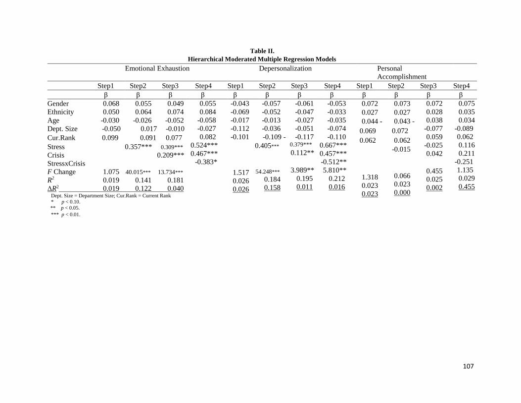
107
Table II. Hierarchical Moderated Multiple Regression Models
Emotional Exhaustion Depersonalization Personal
Accomplishment
Step1 Step2 Step3 Step4 Step1 Step2 Step3 Step4 Step1 Step2 Step3 Step4
β β β β β β β β β β β β Gender 0.068 0.055 0.049 Ethnicity 0.050 0.064 0.074 Age -0.030 -0.026 -0.052 Dept. Size -0.050 0.017 -0.010
Cur.Rank 0.099 0.091 0.077
Stress 0.357*** 0.309*** Crisis 0.209*** StressxCrisis F Change 1.075 40.015*** 13.734*** R2 0.019 0.141 0.181 ΔR2 0.019 0.122 0.040
Dept. Size = Department Size; Cur.Rank = Current Rank * p < 0.10. ** p < 0.05. *** p < 0.01.
0.055 0.084
-0.058 -0.027 0.082
0.524*** 0.467***
-0.383*
-0.043 -0.069 -0.017 -0.112 -0.101
1.517 0.026 0.026
-0.057 -0.052 -0.013 -0.036 -0.109 -
0.405***
54.248***
0.184 0.158
-0.061 -0.047 -0.027 -0.051 -0.117
0.379*** 0.112**
3.989**
0.195 0.011
-0.053 -0.033 -0.035 -0.074 -0.110
0.667*** 0.457*** -0.512** 5.810**
0.212 0.016
0.072 0.027 0.044 -
0.069
0.062
1.318 0.023 0.023
0.073 0.027 0.043 -
0.072
0.062 -0.015
0.066 0.023 0.000
0.072 0.028 0.038
-0.077 0.059
-0.025 0.042
0.455 0.025 0.002
0.075 0.035 0.034
-0.089 0.062 0.116 0.211
-0.251 1.135 0.029 0.455
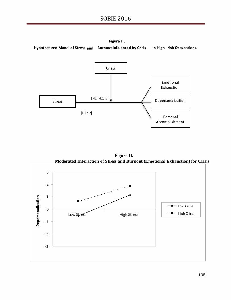
SOBIE 2016
108
Figure II.
Moderated Interaction of Stress and Burnout (Emotional Exhaustion) for Crisis
Figure I .
Hypothesized Model of Stress and Burnout Influenced by Crisis in High - risk Occupations.
[ H1a - c ]
H2, H2a [ - c ]
Crisis
Stress
Emotional Exhaustion
Depersonalization
Personal Accomplishment
-3
-2
-1
0
1
2
3
Low Stress High Stress
Low Crisis
High Crisis

SOBIE 2016
109
Duopoly, Privatization and Environment
Manabendra Dasgupta, University of Alabama at Birmingham
Seung Dong Lee, University of Alabama at Birmingham
Abstract:
We use a segmented market model to analyze the impact of privatization on environment and trade policy.
In particular, we use a quantity setting mixed duopoly model to analyze the effect of privatization on
strategic trade-off between environmental policy and trade policy where the welfare maximizing government
imposes an emission standard instead of a pollution tax as the instrument of environmental policy.
Introduction
The literature on strategic environmental policy has analyzed the effect of free trade and
privatization on environment (Antweiler et al (2001), Barrett (1994), Burguet and Sempere (2003),
Hamilton and Requet (2004), Kennedy (1994), Tanguay (2001), Ulph (1996) and Walz and
Wellisch (1997), Ohori (2004, 2006), Serizawa (2000), Sturm (2001)). In particular, using a two
country - one good duopoly model, they investigated whether free trade and environmental laws are
compatible with each other. Authors such as Barrett (1994), Kennedy (1994) and Tanguay (2001)
have found that trade liberalization may lead to “ecological dumping” or lowering of environmental
tax. In the absence of tariff, optimal environmental tax is lower than efficient tax which is equal to
marginal damage. When tariff is removed environmental tax may act as a rent extracting instrument
in place of tariff. In other words, by lowering tax environmental policy is being used as a substitute
for trade policy to provide domestic firm a competitive advantage. Although this result was the
dominant one, others such as Burguet and Sempere (2003) have found that environmental tax may
increase under certain condition. A bilateral reduction in tariff will increase output and lower price.
But it also increases damage to the environment. This reduces incentive to use environmental policy
strategically to gain competitive advantage and increases incentive for higher environmental
protection and higher tax. Hence, under certain conditions trade policy and environmental policies
may not be strategic substitute.
Several authors, in an effort to extend the literature, also analyzed the effect of privatization of
public enterprises on environmental and trade policies (Barcena-Ruiz and Garzon (2006), Fjeill and
Pal (1996), Ohori (2004), Serizawa (2000)). Investigation of the effects of privatization of public
enterprises on environment and welfare has gained momentum in view of global move towards free
trade. Barcena-Ruiz and Garzon (2006) and Ohori (2004), using a mixed oligopoly model with one
private and one public firm, have shown that while environmental tax is lower than marginal
damage regardless of whether public firm is privatized or not, privatization raises both tax and
tariff. On the one hand, under privatization, government has an incentive to protect newly

SOBIE 2016
110
privatized domestic firm by lowering environmental tax and consequently raising output and profit,
it also has an incentive to protect environment by raising environmental tax.
In this paper we extend the mixed oligopoly model where a welfare maximizing public firm
competes with a profit maximizing private firm by incorporating emission standard as a tool of
environmental policy. The objective is to analyze the impact of privatization on environmental and
trade policy within the framework of an international mixed duopoly. In an earlier paper (Dasgupta
and Lee (2013)) we have shown that although privatization raises environmental tax confirming
results obtained by Ohori (2004) and Barcena-Ruiz and Garzon (2006) tariff may or may not
increase. In this paper we analyze the effect of privatization on the tradeoff between environmental
and trade policies. Specifically, we investigate whether environmental policy and trade policies are
strategic substitutes after public firm has been privatized.
The paper is organized as follows. In second and third section we present the basic model and a
summary of the results related to environmental tax, respectively. The results presented in section 3
are those presented in Dasgupta and Lee (2013) In section 3, we consider only trans-boundary
pollution. Note that if local pollution is considered instead of trans-boundary pollution then results
are strengthened (see Ohori (2004)). In section 4, emission standard replaces pollution tax as the
instrument of environmental policy. We show that while the trade-off between environmental
policy and trade policy still holds before privatization if the damage is sufficiently small the same
level of damage may not guarantee the trade-off after privatization. Finally, in section 5 we offer
some concluding remarks.
The Model
We consider a segmented market or reciprocal dumping model of trade with two countries
(Brander and Krugman (1983), Ohori (2004), Tanguay (2001)). In each country, government sets
pollution tax, e, and tariff, t, to control environment and import respectively. Firms in home country
(1) and foreign country (2) produce a homogeneous output, Q, for home and foreign markets. Each
unit of output generates one unit of pollution. Total production by firm i, i=1,2, j
i
j
i qQ
Where i
jq represents output produced in country i sold in country j. Without loss of
generality we assume that firm in home country (country1) is the welfare maximizing public firm
while firm in foreign country (country 2) is a profit maximizing private firm. After privatization,
both firms maximize profit. Letting total consumption, 2,1, jiqQj
j
ij, the linear demand
function is given by ji QaP where a represents the choke price or the price intercept of the
demand function. We let c denote constant marginal cost which is identical for both firms. Also, it
and ie represent tariff and environmental tax respectively. Profit for firm jijii ,2,1,,
i
j
i
ji
i
j
i
i
j
i
j
ii qtecqakqecqa
(1)
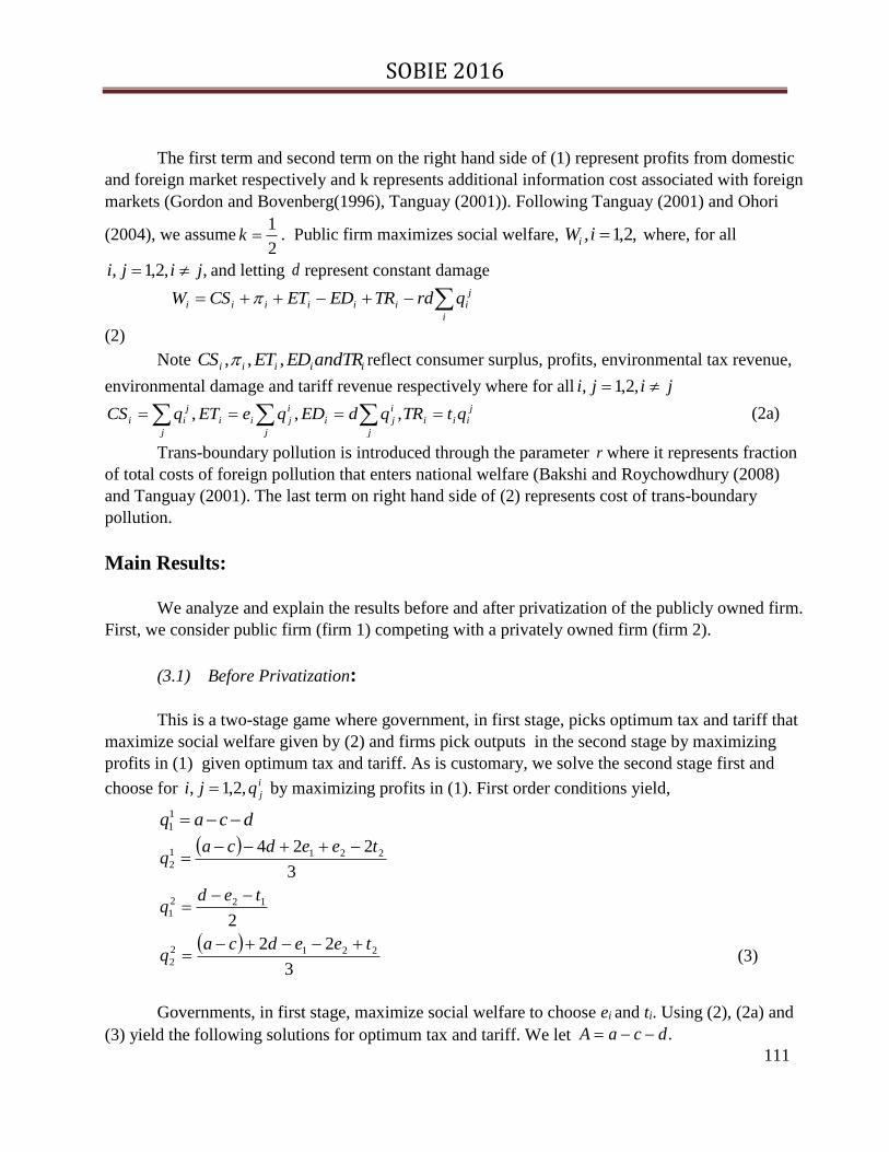
SOBIE 2016
111
The first term and second term on the right hand side of (1) represent profits from domestic
and foreign market respectively and k represents additional information cost associated with foreign
markets (Gordon and Bovenberg(1996), Tanguay (2001)). Following Tanguay (2001) and Ohori
(2004), we assume2
1k . Public firm maximizes social welfare, ,2,1, iWi where, for all
,,2,1, jiji and letting d represent constant damage
i
j
iiiiiii qrdTREDETCSW
(2)
Note iiiii andTREDETCS ,,, reflect consumer surplus, profits, environmental tax revenue,
environmental damage and tariff revenue respectively where for all jiji ,2,1, j
iii
j
i
ji
j
i
jii
j
j
ii qtTRqdEDqeETqCS ,,, (2a)
Trans-boundary pollution is introduced through the parameter r where it represents fraction
of total costs of foreign pollution that enters national welfare (Bakshi and Roychowdhury (2008)
and Tanguay (2001). The last term on right hand side of (2) represents cost of trans-boundary
pollution.
Main Results:
We analyze and explain the results before and after privatization of the publicly owned firm.
First, we consider public firm (firm 1) competing with a privately owned firm (firm 2).
(3.1) Before Privatization:
This is a two-stage game where government, in first stage, picks optimum tax and tariff that
maximize social welfare given by (2) and firms pick outputs in the second stage by maximizing
profits in (1) given optimum tax and tariff. As is customary, we solve the second stage first and
choose for i
jqji ,2,1, by maximizing profits in (1). First order conditions yield,
dcaq 1
1
3
224 2211
2
teedcaq
2
122
1
tedq
3
22 2212
2
teedcaq
(3)
Governments, in first stage, maximize social welfare to choose ei and ti. Using (2), (2a) and
(3) yield the following solutions for optimum tax and tariff. We let .dcaA

SOBIE 2016
112
11
5.0
11
21
rdAde
de211
5.3
11
3 rdA
11
5.8
111
rdAt
2t22
6
11
2 rdA (4)
It is clear that ie < d for 2,1i . This implies that optimal environmental tax is less than
marginal damage. The result is consistent with Ohori (2004).This is the “rent-shifting” effect.
Government has an incentive to use environmental tax to extract economic rent and give domestic
industry competitive advantage. The presence of publicly owned firm does not change the results
obtained in the literature on strategic environmental policy (Barrett (1994), Kennedy (1994)).
Comparing with results obtained by Ohori (2004) we observe that trans-boundary pollution lowers
environmental tax even further, strengthening the “rent shifting” effect. Also, from (4), 12 ee
regardless of whether trans-boundary pollution is considered. However, in presence of trans-
boundary pollution, 12 tt if rddca 5.2 . If r=0 the result coincides with Ohori (2004).
From (3), environmental tax in home country (country 1) raises home production and lowers
production in foreign country (country 2). Therefore, higher tax will shift output from foreign firm
to domestic firm. This gives the domestic government an incentive to set tax at a relatively high
level. However, in foreign country a lower tax implies higher output. Therefore, foreign
government has an incentive to set tax at a relatively low level to offset the rent shifting effect. Note
that, from (3), relatively high tax set by home country also lowers consumption of domestically
produced good in foreign country. Therefore, foreign government has an incentive to set tariff at a
high level to protect domestic market and discourage import. Finally, if trans-boundary pollution is
low enough, that is if
d
dcar
5.2
, then home country may benefit by setting a relatively low
tariff. This is due to what Tanguay (2001) calls pollution shifting effect where home country prefers
having output produced abroad and importing to producing at home since 1r . Substituting ie and
it for ,2,1i from (4) in (3) we get,
11
5.2
11
2
1
rdAq
11
5.51
2
rdq

SOBIE 2016
113
11
5.4
11
72
2
rdAq (5)
Comparing (5) with results obtained by Ohori (2004), It is clear that optimal exports
decrease due to trans-boundary pollution. Therefore, for a given level of damage, higher trans-
boundary pollution will lower export and raise home consumption of domestically produced good.
Note that home consumption of publicly owned firm’s output is independent of trans-boundary
pollution since dcaq 1
1 from (3).
(3.2) After Privatization:
In the second stage, both firms maximize profit. Differentiating (1) with respect to i
jq for
,2,1, ji and using the first order conditions we get, after letting superscript represent optimal
values after privatization,
3
2 1211
1
teecaq P
3
22 2211
2
etecaq P
3
22 1122
1
etecaq P
3
2 2122
2
teecaq P
(6)
From (6), we observe that environmental tax lowers domestic output and raises foreign
output. Tax also raises import. Tariff, on the other hand lowers import and raises domestic output.
In order to determine the effects of privatization on tax and tariff we solve the first stage where
governments choose optimal tax and tariff by maximizing welfare. Differentiating (2) yields after
substituting from (6) in the first order conditions, for ,2,1i
15
8
6
rdAdeP
i
3
2
3
rdAt P
i (7)
Optimal tax continues to be less than marginal damage. Also optimal tariff is strictly
positive. Hence, presence of trans-boundary pollution does not alter the “rent shifting” effect that
holds before privatization. Comparing (7) with (4), it is clear that privatization raises environmental
tax in both countries unambiguously. This result is consistent with that obtained in Ohori (2004).

SOBIE 2016
114
This implies that incentive to use tax as a rent shifting tool is much stronger before privatization
than it is after privatization. Comparing tariffs we get, from (7) and (4), 22 tt P but 11 tt P only if
d
Ar
3 . Although privatization raises tariff in country 2, it does so in country 1 only if trans-
boundary pollution is sufficiently low. In this case, both countries are willing to use tariff as a rent
shifting tool rather than environmental tax. From (6), higher environmental tax raises import and
lowers domestic production. If r is sufficiently low, import is particularly attractive relative to
domestic production. To protect domestic firm and transfer rent from foreign producers to domestic
producer government has an incentive to raise tariff. However, for a high level of trans-boundary
pollution, import may no longer be attractive relative to domestic production and hence there may
no longer be a need to protect domestic firm by raising tariff. Therefore if d
Ar
3 then 11 tt P .
Intuitively, it will be clear once we examine optimal output after privatization. Substituting optimal
tax and tariff from (7) in (6) we get, for jiji ,2,1,
rdA
q i
i45
2
2
45
28
6
rdAq i
j (8)
We observe from (8) that higher trans-boundary pollution raises consumption of
domestically produced goods and lowers import. Therefore, in presence of high trans-boundary
pollution, the incentive to raise tariff to lower import and use tariff as a rent shifting tool decreases.
That job is being accomplished by trans-boundary pollution.
Duopoly with Emission Standard
We assume firm 1 is welfare maximizing publicly owned firm and firm 2 is profit maximizing
private firm. We also allow firms 1 and 2 to represent countries 1 and 2, home and foreign
respectively. For i= 1, 2 , production generates emissions according to 𝛼 = 𝑄𝑖 – a where 𝛼 represents
emissions and a is abatement. The abatement costs are given by 𝑍 =𝑎2
2. Emissions cause purely local
damage. The damage function is 𝐷(𝛼) =𝑑𝛼2
2 𝑤ℎ𝑒𝑟𝑒 𝑑 is the damage parameter. Following Strum
(2001) we normalize constant cost to zero. In the second stage firms choose 𝑞𝑖𝑗 for 𝑖, 𝑗 = 1,2 by
maximizing for jijii ,2,1,, , 𝜋𝑖 = [𝐴 − ∑ 𝑞𝑖𝑗
𝑗 ]𝑞𝑖𝑖 + 𝑘[𝐴 − ∑ 𝑞𝑗
𝑖𝑗 − 𝑡𝑗]𝑞𝑗
𝑖 −1
2(𝑄𝑖 − 𝛼𝑖)
2.
(9)
In the first stage, government chooses 𝛼 and 𝑡 by maximizing, for 𝑖 = 1,2,
𝑊𝑖 = 𝐶𝑆𝑖 + 𝜋𝑖 + 𝑇𝑅𝑖 −1
2𝑑𝛼2 (10)

SOBIE 2016
115
(4.1) Before Privatization:
As is customary, we solve the second stage first. Differentiating (9) and (10) respectively with
respect to 𝑞𝑖 2 𝑎𝑛𝑑 𝑞𝑖
1 𝑓𝑜𝑟 𝑖 = 1,2 and solving the first order conditions yield,
𝑞11 =
17𝐴 + 11𝛼1 + 2𝛼2 + 𝑡1 + 7𝑡2
28
𝑞21 =
−4𝐴 + 8𝛼1 − 4𝛼2 − 2𝑡1 − 14𝑡2
28
(11)
𝑞12 =
10𝐴 + 14𝛼1 − 𝛼2 − 𝑡1 − 5𝑡2
28
𝑞22 =
9𝐴 − 7𝛼1 + 17𝛼2 + 5𝑡1 + 7𝑡2
28
From (11), we observe that higher tariff lowers import and vice versa. However, effect of
tariff on total output requires explanation. Note that total output produced by firm i is 𝑄𝑖 = ∑ 𝑞𝑗𝑖
𝑗
For firm 2 higher tariff (𝑡2) lowers import and raises output. For profit maximizing firm 2,
higher output is consistent with higher profit. However, for firm 1 higher tariff (𝑡1) lowers both import
and total output. As tariff is raised the welfare maximizing firm has an incentive to raise output since
it increases profit and welfare. But higher output also raises environmental damage and lowers
welfare. In this case, pollution effect (environmental damage) dominates profit. Hence, total output
decreases as tariff is raised. It is also clear from (11) that as emission increases total output in both
home and foreign countries would increase. This is not surprising since both raising emission and
lowering of environmental tax represent laxer environmental standard. However, a closer look makes
it clear that as emission is raised at home (𝛼1) not only will home output and output sold by home
public firm in foreign country increase but also there is a decrease in foreign consumption of its own
output produced by privately owned firm (𝑞22). This implies home government uses emission as a
strategic instrument to expand market share for its own public firm. The result is consistent with Ohori
(2004) where the instrument of choice was environmental tax.
We now investigate whether trade liberalization leads to lowering of environmental standard.
In other words, we check if a lower tariff will raise emission level. We solve the first stage by
choosing 𝛼𝑖 𝑓𝑜𝑟 𝑖 = 1, 2 maximizing 𝑊𝑖 𝑓𝑜𝑟 𝑖 = 1,2 from (10) after substituting for 𝑞𝑖𝑗𝑓𝑜𝑟 𝑖, 𝑗 =
1, 2 in (10). The first order conditions are as follows:
𝜕𝑊1
𝜕𝛼1= 985𝐴 + (995 − 1568𝑑)𝛼1 + 5𝛼2 + 394𝑡1 + 384𝑡2 = 0

SOBIE 2016
116
𝜕𝑊2
𝜕𝛼2= 37𝐴 − 197𝛼1+(745-1568d)𝛼2 + 207𝑡1 + 25𝑡2 = 0
(12)
Equation (12) shows that trade liberalization (lower tariff) raises emission level (ℎ𝑖𝑔ℎ𝑒𝑟 𝛼)
provided level of damage is sufficiently low. If d < 995
1568 𝑎𝑛𝑑 𝑑 <
745
1568 for countries 1 and 2
respectively then trade policy and environmental policies are strategic substitutes. This implies that
one of the fundamental results obtained in the literature on strategic environmental policy holds even
if environmental tax is replaced by emission level as the instrument of environmental policy.
However, if d > 995
1568 and d >
745
1568 the damage may be too high for countries 1 and 2 respectively to
use environmental policy as a rent extracting tool.
(4.2) After Privatization: In the second stage both firms choose output by maximizing profit given by (9) while governments choose
optimal tariff and emission standard in the first stage by maximizing welfare given by (10). We solve the
second stage first to get, for all 𝑖, 𝑗 = 1, 2 𝑎𝑛𝑑 𝑖 ≠ 𝑗
𝑞𝑖𝑖 =
𝐴 + 𝑡
2
(13)
𝑞𝑗𝑖 =
4𝛼 − 7𝑡 − 3𝐴
2
Equation (12) shows that a lower tariff raises import and vice versa. A lower tariff also raises total
output and consumption of domestically produced goods. These results are the same as those
obtained in the previous section where a public firm was competing against a privately owned firm.
Also, a laxer environmental standard represented by higher 𝛼 raises output and vice versa. The
relation between output and emission standard remains the same after public firm has been
privatized. Higher output implies higher profit. But it also so means higher damage. Profit
consideration dominates environmental consideration. This is particularly true when both firms are
privately owned.
We turn to the question of whether there is a trade-off between tariff and emission level chosen by
the welfare maximizing government. Differentiating 𝑊𝑖 with respect to 𝛼𝑖, i= 1, 2 and setting it to
zero we get,
(12 − 2𝑑)𝛼𝑖 −47
2𝑡𝑖 − 8𝐴 = 0
(14)
From (14) it is clear that if 𝑑 < 6 a lower tariff will lead to a choice of a lower emission level.
Hence trade liberalization may not lead to a laxer environmental standard. This result is similar to
that obtained by Burguet and Sempere (2003) where the instrument of environmental policy was
pollution tax. From (11), a lower tariff raises output, But it also increases damages to the

SOBIE 2016
117
environment reducing the incentive to choose a higher emission level. However, as tariff is
removed tariff revenue decreases and import becomes relatively less attractive and export becomes
relatively more attractive. This raises the incentive to increase domestic output by choosing a higher
emission level and a laxer environmental standard. If 𝑑 < 6 then there may not be a trade-off
between tariff and emission level. Note that if damage per unit is sufficiently high (𝑑 > 6) then it is
clear that trade liberalization will lead to a choice of a laxer environmental standard.
Conclusion:
We have analyzed the effect of privatization on the trade-off between trade policy and
environmental policy where instruments of trade policy and environmental policy are tariff and
emission level respectively. We have shown that in a mixed duopoly model governments have an
incentive to use environmental policy as a strategic substitute for trade policy if damage is
sufficiently low (𝑑 <745
1568 ). However, from (14) it is clear that same condition is not enough to
guarantee trade-off when the publicly owned firm is privatized. Therefore, relative to mixed
duopoly it will take a much higher damage per unit in market with two privately owned firm for the
governments to use environmental policy strategically as a rent extracting tool.
SOBIE 2016
118
References:
1. Antweiler,W, B.R. Copeland and M. S. Taylor. “Is Free Trade Good for Environment?”
American Economic Review, 2001, Vol. 91, 877 – 908.
2. Bakshi, Soham and Amrita Ray Chowdhury. “Trans-boundary Pollution, Trade
Liberalization and Environmental Taxes” Mimeographed. 2008. Tilburg University.
3. Barcena-Ruiz, Juan Carlos and Maria Garzon. “Mixed Oligopoly and Environmental
Policy” Spanish Economic Review, 2006, Vol. 8, 139 – 160.
4. Barrett, S. “Strategic Environmental Policy and International Trade” Journal of Public
Economics, 1994, Vol. 54, 325 – 338.
5. Brander, J and P. Krugman. “A Reciprocal Dumping Model of International Trade” Journal
of International Economics, 1983, Vol. 17, 313 – 321.
6. Burguet R and J. Sempere (2003) “Trade Liberalization, Environmental Policy and
Welfare”. Journal of Environmental Economics and Management 46: 25-37.
7. Dasgupta,M. and S.D.Lee. “Mixed Oligopoly, Trade and Environment” SOBIE:
Proceedings of Annual Meetings, 2013.
8. Fjell,K and D. Pal. “A Mixed Oligopoly in the presence of Foreign Private Firms”
Canadian Journal of Economics, 1996, Vol. 29, 737 – 743.
9. Gordon, R. H and A. L. Bovenberg. “Why Capital is so Immobile Internationally? Possible
Explanation and Implication for Capital Income Taxation.” American Economic Review,
Vol. 86, 1057 – 1075.
10. Hamilton, S and T. Requate.”Vertical Structure and Strategic Environmental Policy”
Journal of Environmental policy and Management, 2004, Vol. 47, 260 – 269.
11. Kennedy, P. W. ”Equilibrium Pollution Taxes in Open Economies with Imperfect
Competition”, Journal of Environmental Economics and Management, 1994, Vol. 27, 49 –
63.
12. Ohori, Shuichi. “Environmental Tax, Trade and Privatization” The Kyoto Economic Review,
2004, Vol. 73, 109 -120.
13. Ohori, Shuichi. “Optimal Environmental Tax and Level of Privatization in an International
Duopoly” Journal of Regulatory Economica,2006, Vol. 29, 225 – 233.
14. Serizawa, N. “Optimal Trade Policy in an International Mixed Oligopoly” Seoul Journal of
Economics, 2000, Vol. 13, 107 – 122.
15. Sturm, D. “Choosing How to Compete: Is Environmental Policy the Optimal Instrument?”
Discussion paper; 2001, London School of Economics.
16. Tanguay, G. “Strategic Environmental Policies under International Duopolistic
Competition”, International Tax and Public Finance, 2001, Vol.8, 793 – 811.
17. Walz U and D. Wellisch (1997) “Is Free Trade in the Interest of Exporting Countries When
There is Ecological Dumping?” Journal of Public Economics 66: 275-291.

SOBIE 2016
119
ABSTRACTS

SOBIE 2016
120
Social Media: Education to Business
William Piper, Alcorn State University
Pj. Forrest, Alcorn State University
Extended Abstract
The last two decades have seen traditional media transformed into new channels that encompass
digital, computerized, and networked information and communication technologies (Eid,Ward
2009.) We know them as Social Media (SM) that our current generation of students, Millennial’s ,
as the future generation of business operatives, will be using social media to research, identify work
related situations, run the business and communicate with coworkers, clients, consumers and
competitors. They primarily use Facebook and Twitter in school, but quickly learn that email and
Linked-in are the business platforms most used in the business world. There are still many
professors who consider Social Media to be a fad and a detraction and try their best to keep it out of
there classes. But the time has come to accept that SM is here to stay, and to embrace it as a new
and effective teaching tool.
Technology is the best way to connect with Millennia’s in school and in the business world. Social
media is being taught and used even in 1st grade classrooms (@coolatteacher.) Social media has
been shown to be the best way to teach our students, and they also learn the power and importance
of social media for business. Classroom applications and exercises in Social Media not only helps
them learn but gives them practice for business applications. Social Media skills have been
considered the most important skill sought for by employers (Afshar.) Students today, both at the
graduate and undergraduate level, are being hired as Social Media Directors (Clampitt, 2017)
Students that are not familiar with or do not use Social Media (SM) will not progress in business as
quickly. As part of their business curriculum students should be required to create and use
Facebook, email, Twitter and Linked-in. These are basics for classroom study today and the work
environment tomorrow.
Joshua Waldman in his “Career Enlightenment” Blog compiled statistics from many sources (see
reference list.) Specifically, he confirms that for both personal and business, Email usage is still the
most commonly employed means of business communications with 91.7% using personal accounts
and 89.6% using business accounts. Facebook is a competitive second at 58.5% which is
significant portion of the population. The 7th Annual Social Media Marketing Report of the Social
Media Examiner reported that 96% of the small business participants in their survey used SM, and
92% of them agree or strongly agree the SM was critical for their business.
In business, email is still out performing other media. In the world of Social Media Facebook out-
performs all competitors. In business Facebook is not king but with almost 60% of business people
surveyed using it for business communications that makes Social media an important
SOBIE 2016
121
communications link. The important issue is preparing students for business communications by
creating assignments and projects requiring the use of Social Media and common email usage.
While all students in a class may not bother to obtain a text – they will still have a smart phone.
More and more students are signing into online classes via cell phone or tablet rather than a
computer. It is proposed that, as the cell phone is the primary way students access Social Media,
that it is an excellent way to reach them with the course material as well. In fact, Rheingold reports
that the “Social Media Virtual Classroom Project” (funded by the HASTACC/MacArthur
Foundation Digital Media & Learning competition) is developing a complete Social Media
Classroom which “Social Media Virtual Classroom Project” (funded by the HASTACC/MacArthur
Foundation Digital Media & Learning competition) is developing a complete Social Media
Classroom. Social Media has already invaded our classrooms, we need to use it instead of fighting
it.
Driving this need to teach social media and to use it as a teaching tool, originates from the
importance it has in business, both in promotion and management. Businesses heavily uses SM to
communicate with consumers but also to run the business. 20% of the 340M+ tweets that are sent
each day are business usage. More than 80% of people expect the CEO’s of business to have an
online profile. This raises a company’s profile and makes the brand seem more honest and
trustworthy. (2013 CEO, Social Media and Leadership survey by BRANDfog.)
In today’s business world, companies who do not make use of SM are viewed as outdated, and
beginning to fall behind the competition. Small businesses, who have very small advertising funds,
have used SM to grow and thrive. Social media is an essential part of doing business today.
(Hendricks, Drew http://www.forbes.com/sites/drewhendricks/2014/02/25/3-ways-social-media-
is-driving-a-business-revolution/)
Gen Z will become college juniors next year, and by 2020 will comprise 40% of all U.S.
Consumers. The lives of Gen Z are organized and shaped by what they have on their cellphones.
They use various cellphone apps to organize and control their lives. Gen Z’s have an
entrepreneurial spirit and many want to start their own businesses – based on the information
available at their fingertips via cell phone Their experiences with interactions via their cell phone
with people from other socio/economic backgrounds have made them socially conscious. They
don’t make a sharp distinction between home and work life (Fujioka.)
In addition to email, Facebook, Twitter and Linked-in there are a wide variety of other Social Media
sites, all which have different uses, which can be adapted for classroom use. Googling “using
Social Media to teach” will provide a wealth of information about these sites and how they can be
used. Anyone who has college students, or children of almost any age, know that they constantly
are on their phone. As educators, we should harness this technology and use it to our advantage.
SOBIE 2016
122
References
Eid, Mahmoud and Stephen J. A. Ward. “Ethics, New Media, and Social Networks” Global Media
Journal, Volume 2, Issue 1, pp1-4
@coolatteacher, “Teachers Use Social Media in the Classroom.”
http://www.coolcatteacher.com/10-amazing-ways-teachers-have-used-social-media-to-enhance-
learning/. Downloaded 2/15/2017
Hendricks, Drew http://www.forbes.com/sites/drewhendricks/2014/02/25/3-ways-social-media-
is-driving-a-business-revolution/ downloaded 3/9/2017 at 5pm
Rheinggold, Howard. “Using Social Media to Teach Social Media.” The New England Journal of
Higher Education. Summer 2008, pp. 25-26
2013 CEO, Social Media and Leadership survey by BRANDfog.
http://www.brandfog.com/CEOSocialMediaSurvey/BRANDfog_2013_CEO_Survey.pdf
Waldman, Joshus , Career Enlightenment LLC, https://careerenlightenment.com/infographic-
social-resume-how-job-seekers-and-employers-are-connecting-online, 2016
Ashfar, Vala. The Importance of Social Business Skills, INC, Feb 19, 2017
Clampitt, Phillip. Social Media Strategy, Publication date 2017, Sage Publishing
Stelzner, Michael, 2014 Social Media Marketing Report
http://www.socialmediaexaminer.com/SocialMediaMarketingIndustryReport2014.pdf
Fujioka, Russ. How Gen Z Influencers Think Differently, Inc. Magazine, February 10 2016
http://www.chicagotribune.com/search/dispatcher.front?Query=How+Gen+Z+Influencers+think+
differently&target=all&spell=on

SOBIE 2016
123
$port $ponsorship: Big Money
Pj Forrest, Alcorn State University
Extended Abstract
Introduction The success of sports sponsorship depends on how much money the company earns by paying
the premier athletes millions. The sums athletes are paid for sponsorship are so large that many
people are skeptical that companies can earn back such high amounts. But a quick look at the
numbers shows why. LeBron James was paid $60m/yr., by Nike. Nike earned $400M/yr. on his
shoe line only. James has earned $450m in his career via sponsorship, increasing his sponsors sales
between 10 and 50% each time (Badenhausen.)
James, at $77m is third in total winnings in 2016 behind Cristiano Renaldo ($88m) and Lionel
Messi ($81m) but in endorsements both Renaldo at $32m and Messi at $28m fall far behind James’
$54m https://www.forbes.com/pictures/mli45ffmil/1-cristiano-ronaldo/#34d2c9cd7039
Salary-wise all athletes fall behind boxer Floyd Mayweather, generally considered the worlds
richest athlete with lifetime career earnings totaling $800m by 2017 (Beran) However, the majority
of his wealth is from winnings as he has had, unlike young, richer athletes, few sponsorships
Sports sponsorships have many benefits to offer a company, but perhaps the most beneficial is in
the areas of brand awareness, brand image and connecting with the target market. According to
Butrill sports sponsorship:
a) Provides new advertising channels
b) Able to identify target market and create brand audience alignment
c) Can align with brand image when athletes values embody it. Elevates a brand’s image
by putting a face on those values " Brands must tap into the spirit of the athlete they are
sponsoring, creating campaigns that drive a sense of enthusiasm for the sport not
dependent on their sponsored athlete winning every game.”
d) Athletes come with their own audience thus creating an additional channel if creative development is used to optimize (Buttrill.)
Through its football sponsorship association, Hyundai / Kia Motors positioned itself as a brand that
delivers the excitement of the soccer to fans all over the world, and remains deeply committed to
supporting and furthering the development of the sport by sponsoring FIFA from now through
2022. FIFA to expects to reap US $1.4 billion in sponsorship revenues from Brazil 2014 with 19
additional sponsors. (The Most effective sports marketing & sponsorship: Samsung & Hyundai-
Kia)

SOBIE 2016
124
Difficulty of measuring exact monetary effects
The issue of measuring the monetary effects of sports sponsorship is the same which perplexes any
company trying to measure the exact monetary influence promotion has on sales. There are too
many variables which intervene and very few measures with any degree of exactness. Thus:
-1/3 to ½ of American companies don’t have a comprehensive measure of ROI
-a comprehensive approach can increase returns by as much as 30%
Some measures which may be used are:
a) Cost per reach (Reach calculations should favor exposure to the target demographic over
total numbers.)
b) Unaided awareness per reach (brand awareness, related to leveraging)
c) Sales/Margin per dollar spent, difficult to quantify. Two methods:
d) Tie sponsorship to key qualitative measures such as unaided awareness, etc.. Then track
the impart of each variable on short- and long-term sales
e) Link econometric data such as spending and reach over an extended time, then isolate
the impact of sponsorships
f) Long term brand attributes. “A qualitative assessment or survey can help companies
identify the brand attributes that each sponsorship property supports. Analysis of those
results helps marketers determine which sponsorships are reinforcing a common brand
theme.’
g) Indirect benefits. For example hosting clients at a sporting event.
Positive ROI is more likely for sponsors of better performing teams, sponsors that
affiliate at a high level and sponsors outside the automotive industry. (Analyzing Return-
on-Investment in Sponsorship: Modeling Brand Exposure, Price and ROI in Formula
One Racing)
" The World Cup in Brazil generated $1.4B from sponsorship deals with 20 major
companies, a 10% increase from the 2010 World Cup. Global estimates place revenues
from sports sponsorship rising to beyond $45B by '16.--- Charles Russell Speechlys.
(SBD Global/April 22, 2015/Marketing and Sponsorship)
Risks of sports sponsorship
O.J. Simpson, Tiger Woods, Michael Vick and the list goes on and on. When you designate an
athlete as the face of your product, any misdoings by the athlete may have a negative impact on
your brand. In the 90’s when Simpson was arrested for murder, many of his sponsors such as Hertz
and Samsonite stood by him and were lauded for their loyalty. All of his sponsors finally cancelled
his contracts as his guilt became more evident and he did not get them back, regardless of the not
guilty verdict.
SOBIE 2016
125
The contracts of todays’ most sponsored athletes generally contain a morals clause which allows the
sponsor to end the contract if the athlete is associated with any negative activity. Michael Vick and
Tiger Woods had a different experience than O.J. Simpson. Some of their biggest sponsor’s
dropped them as soon as the negative publicity began, and those that didn’t were criticized by the
public (https://www.thoughtco.com/tiger-woods-dropped-sponsors-1566402,
http://www.cbc.ca/sports/football/sponsors-come-down-hard-on-michael-vick-1.662542.) Another
reason they are dropped so fast is the negative impact on profits. The Tiger Woods scandal of 2009
purportedly cost his sponsors a collective $5 to $12 billion. It was estimated that it reduced
shareholder values in the sponsoring companies by 2.3%.
Will sports sponsorship continue?
Almost certainly. For many sports, NASCAR for example, the team or athlete and the sponsor
were intimately linked from the beginning. Many companies have learned that sports sponsorship
it the best method to achieve brand awareness and gain a higher profile, to revive a failing or
negative brand image, to project a specific brand image or better reach their target markets. Sports
sponsorship can give a higher profile for the teams and athletes, but also means a great deal of
money. And right now sports sponsorship is big money for both athletes and business.

SOBIE 2016
126
The Role of Foundations in Entrepreneurial Activities
Eren Ozgen
Troy University, Dothan Campus
Abstract
Entrepreneurship is considered crucial in economic growth and job creation. To date within a
multidisciplinary theoretical framework the role of foundations in entrepreneurial activities is
relatively less studied. Foundations could be valuable in mobilizing resources and disseminating them
in supporting entrepreneurship development despite continuous change in economic, cultural and
technological conditions. In this paper based on an interdisciplinary theoretical context a few critical
roles of foundations in entrepreneurial activities will be highlighted to identify best practices and
critical domains in which foundations support and foster entrepreneurial activities. The paper will
also present propositions, future research areas and implications.

SOBIE 2016
127
Female Entrepreneurs In Developing Countries: What Could Be
Possible Challenges?
Eren Ozgen
Troy University, Dothan Campus
Abstract
Female entrepreneurial activity varies in developed versus developing countries. To date most
literature on female entrepreneurship has been focused on developed countries and contingency
studies on female entrepreneurial activities in developing countries are rather limited. There is also
a need to build more theoretical explanations for female entrepreneurial activities in various
contexts and contents. Based on an integrative theoretical structure the paper aims to bring an
understanding on possible obstacles for female entrepreneurial activities in developing countries.
The study suggests that by exploring numerous external factors and underpinning crucial
impediments for female entrepreneurial activities in developing countries it may be easier to offer
assistance and develop policy implications for female entrepreneurial activity in a cross country
research.
SOBIE 2016
128
Personal Knowledge Management (PKM) and the Leadership
Development of African-American Women Leaders: A Narrative
Inquiry
Kimberly L. Wright, University Of Phoenix
Abstract
The lack of diversity in corporate leadership positions, especially among African- American
women, has garnered significant research and attention in various industries. The research purpose
sought to examine how the underrepresentation of African- American women in leadership roles
influenced the personal knowledge management (PKM), leadership development, and motivation to
lead (MTL) of African-American women leaders. Qualitative method and a narrative design inquiry
was used to explore participants’ personal and professional experiences before and after formal
leadership attainment. The narrative design included interviewing a small cross-section of six
African-American women serving in leadership roles throughout the New York tristate area (New
York, New Jersey, and Connecticut). The sample participants were individually interviewed in a
face-to-face setting, using semi-structured and open-ended questions that focused on personal and
professional experiences related to leadership skills. Specific themes of positioning were discovered
fundamental to the leadership experiences of the African-American women participants. Access to
higher education, membership in social organizations, community service involvement, and
workplace challenges, to include the application of an assertive personality were found to be
common leadership influences among the participants. Findings in this study may proffer
organizational leaders with the insight needed for promoting best practices of diversity and
inclusion initiatives targeting African American women or other minority population groups for
leadership roles.