snow-to-liquid ratio variability and prediction at a …
TRANSCRIPT

SNOW-TO-LIQUID RATIO VARIABILITY AND PREDICTION
AT A HIGH-ELEVATION SITE IN UTAH’S
CENTRAL WASATCH MOUNTAINS
by
Trevor Iain Alcott
A thesis submitted to the faculty of The University of Utah
in partial fulfillment of the requirements for the degree of
Master of Science
Department of Atmospheric Sciences
The University of Utah
August 2009

Copyright © Trevor Iain Alcott 2009
All Rights Reserved

ABSTRACT
Modern snowfall forecasting is a three-step process involving a quantitative
precipitation forecast (QPF), determination of precipitation type, and application of a
snow-to-liquid ratio (SLR). The final step is often performed using climatology or
unverified empirical techniques. Based on a record of consistent and professional daily
snowfall measurements, this study 1) presents general characteristics of SLR at Alta,
Utah, a high-elevation site in interior North America with frequent winter storms, 2)
diagnoses relationships between SLR and meteorological conditions using reanalysis
data, and 3) develops a statistical method for predicting SLR at the study location.
The mean SLR at Alta is similar to that observed at lower elevations in the
surrounding region, with substantial variability throughout the winter season. Using data
from the North American Regional Reanalysis, temperature, relative humidity and wind
speed are found to be related to SLR, the strongest correlation occurring with 650-hPa
temperature. A stepwise multiple linear regression (SMLR) equation is constructed that
explains 68% of the SLR variance for all events, and 88% for a high SWE (>25 mm)
subset. Applying the SMLR approach to archived 12-36 h forecasts from the National
Centers for Environmental Prediction Eta/North American Mesoscale model yields an
improvement over existing operational SLR prediction techniques, although errors in
QPF over complex terrain can limit skill in forecasting snowfall amount.

TABLE OF CONTENTS
ABSTRACT....................................................................................................................... iv
LIST OF FIGURES .......................................................................................................... vii
ACKNOWLEDGEMENTS............................................................................................... ix
1. INTRODUCTION ........................................................................................................1
1.1 Background .......................................................................................................1 1.2 Objectives .........................................................................................................7
2. DATA AND METHODS ...........................................................................................10
2.1 Snowfall Observations ....................................................................................10 2.2 Quality Control and Sources of Error .............................................................11 2.3 Upper-Air Data ...............................................................................................12 2.4 Stepwise Multiple Linear Regression Procedure............................................13
3. RESULTS ...................................................................................................................16
3.1 General SLR Characteristics at Alta ...............................................................16 3.2 Relationships Between SLR and Local Atmospheric Conditions ..................20
3.2.1 Vertical Profiles ...............................................................................20 3.2.2 Near-Crest-Level Temperature ........................................................23 3.2.3 Near-Crest-Level Wind Speed.........................................................25 3.2.4 SWE .................................................................................................28 3.2.5 Surface Temperature........................................................................30 3.2.6 Other Processes................................................................................33
3.3 Diagnosis and Prediction of SLR....................................................................34 3.3.1 Stepwise Multiple Linear Regression using Reanalysis ..................34 3.3.2 Application to Eta/NAM Forecasts..................................................41
4. Conclusions.................................................................................................................46
4.1 Summary .........................................................................................................46

vi
4.2 Future Work ....................................................................................................48
REFERENCES ..................................................................................................................50

LIST OF FIGURES
Figure Page
1.1. The Alta-Collins snow study site.............................................................................6 1.2. Verification of National Weather Service Cottonwood Canyons probabilistic snowfall forecasts....................................................................8 3.1. Histogram of observed SLR values for all events .................................................17 3.2. Box-and-whisker plot of SLR for all events ..........................................................19 3.3. Vertical profiles of linear correlation coefficient between SLR and atmospheric variables for all events...........................................................21 3.4. Vertical profiles of linear correlation coefficient between SLR and atmospheric variables for high SWE events ..............................................22 3.5. SLR versus 650-hPa temperature...........................................................................23 3.6. Probability density function of the lowest and highest fifths of 650-hPa temperature ..................................................................................26 3.7. SLR versus 650-hPa wind speed............................................................................26 3.8. Probability density function of the lowest and highest fifths of 650-hPa wind speed. ..................................................................................27 3.9. SLR versus SWE....................................................................................................29 3.10. Probability density function of the lowest and highest fifths of SWE...................29 3.11. SWE versus 650 hPa temperature for all events....................................................31 3.12. SWE versus 650 hPa wind speed for all events.....................................................31 3.13. Observed SLR and SLR indicated by the NWS MCT versus surface temperature for all events ..............................................................32

viii
3.14. Results of the stepwise multiple linear regression for all events when run using all potential predictors (test 1a)........................................37 3.15. Results of the stepwise multiple linear regression for high SWE events when run using all potential predictors (test 1b) ............................37 3.16. Results of the stepwise multiple linear regression for all events when run using only temperature and wind predictors (test 2b)................40 3.17. Results of the stepwise multiple linear regression for high SWE events when run using only temperature and wind predictors (test 2d) .....................................................................................40 3.18. Observed versus forecast SLR for an independent set of 176 events, using Eta/NAM temperature and wind predictors .....................................43 3.19. Observed precipitation versus NWS Alta grid point QPF. ....................................45

ACKNOWLEDGEMENTS
I thank my advisor, Jim Steenburgh, for his support and guidance throughout this
entire project, and my other two committee members, John Horel and Larry Dunn, for
their comments and suggestions in the realms of statistics and operational forecasting.
This research was based in part on work supported by a series of grants provided by the
National Oceanic and Atmospheric Administration CSTAR program and National
Science Foundation grant ATM-0627937.
I also thank Alta ski area, the Alta snow safety patrol, General Manager Onno
Wieringa, Snow Safety Director Titus Case, Assistant Snow Safety Director Daniel
“Howie” Howlett for collecting and providing the Alta snow data, and Randy Graham of
NWS Salt Lake City for offering input and assistance with obtaining archived NWS
forecasts. Mike Kok offered input as an experienced Cottonwood Canyons snow
forecaster, Greg West helped with the use of grid analysis software and the North
American Regional Reanalysis, and other University of Utah graduate students provided
a sounding board for ideas on many occasions. Thank you for making this work possible.

CHAPTER 1
INTRODUCTION
Background
Winter precipitation forecasting typically involves three steps: (1) production of a
quantitative precipitation forecast (QPF), (2) determination of precipitation type and (3)
application of a snow-to-liquid ratio (SLR1) if snow is expected to be the dominant
precipitation type. The resulting quantitative snowfall forecast (QSF) is the product of
QPF and SLR. This process may be reduced to two steps by including precipitation type
in an SLR algorithm (Dubé 2008). In addition to QPF uncertainties, large inter- and
intrastorm SLR variability is a major contributor to QSF error. For example, 6-h SLR
observed at National Weather Service (NWS) offices ranges from 1.9 to 47 (Roebber et
al. 2003), whereas daily SLR in the central Rocky Mountains ranges from 3.9 to 100
(Judson and Doesken 2000). Given these wide ranges, even perfect QPF is often of
limited value if an incorrect SLR is applied. The continued use of unproven empirical
techniques to predict SLR led Roebber et al. (2003) to describe this portion of the winter
precipitation forecast process as “largely a non-scientific endeavor.”
1 Of several means to quantify snow character (e.g., density, percent water content, specific gravity, SLR), this work is concerned with SLR, defined as the ratio of the depth of new snowfall to the depth of melted liquid equivalent, due to its relevance in operational forecasting. An SLR of 12.5 corresponds to a snow density of 80 kg m-3, an 8% water content, and a specific gravity of 0.08.
2
SLR depends on the fraction of void space within a sample of snow, a property
controlled by ice crystal size and shape (habit), riming, aggregation, sublimation or
melting of exterior crystal branches at the surface and aloft, mechanical fragmentation by
strong winds, rain falling on snow and vapor diffusion during metamorphosis on the
ground (Roebber et al. 2003, Baxter et al. 2005, Dubé 2008). These processes can be
viewed in a top-down manner following an ice crystal from formation in a cloud to
settlement on the ground. Crystal habit can serve as a first guess for SLR, as shown in
the physically-based algorithm developed by Dubé (2008). Nakaya (1954) found that
crystal type is determined primarily by temperature, with the exception of the −14° to
−17°C range where supersaturation with respect to ice controls a shift from plates to
dendrites. Observational studies by Power et al. (1964) and Dubé (2008) found the
highest SLR values for dendrites (19 to 25) and the lowest for columns (10 to 11),
although Nakaya (1954) found SLR values up to 100 for dendritic snowfalls in low wind
conditions immediately after accumulation.
During or after depositional crystal growth, riming can fill pore space and
decrease SLR by 50% or more (Power et al. 1964). Aggregation of multiple crystals can
lead to higher SLR values (Dubé 2008). Falling crystals may encounter regions of
above-freezing temperatures or subsaturation with respect to ice, which further decrease
SLR by melting and/or sublimation (Roebber et al. 2003). Once near or at the ground,
surface wind speeds above 8 m s-1 transport snow and reduce SLR by mechanically
removing outer crystal branches (Li and Pomeroy 1997, Roebber et al. 2003, Dubé 2008).
Sublimation or melting on the ground can further decrease SLR, as does rain on snow,
which adds mass while maintaining or decreasing depth. Compaction due to the added

3
weight of overlying snow is thought to reduce SLR during high snow water equivalent
(SWE) events (Judson and Doesken 2000, Roebber et al. 2003, Ware et al. 2006, Dubé
2008), but experiments by Gunn (1965) involving adding weights to a snow surface
suggest that such effects are small. Snow metamorphism, driven by vertical temperature
gradients and/or Kelvin effects, results in more rounded forms with lower SLR and can
begin while snow is still accumulating (Doesken and Judson 1997).
The complexity of the snow formation process has prompted forecasters to take a
variety of approaches to SLR prediction, including climatological, statistical and
physically based methods. The commonly accepted “ten-to-one rule” for SLR is thought
to have originated from a climatology in the mid-19th century (Roebber et al. 2003), and
problems with this approach were noted well over a century ago due to the large temporal
and spatial variability in SLR (Abe 1888). Based on SLR observations from Cooperative
Observer stations (COOP) across the United States, Baxter et al. (2005), found that SLR
varies regionally and suggests that 13 is more appropriate if a fixed ratio is desired.
Various empirical prediction methods relate SLR to temperatures at the surface or
aloft. Bossolasco (1954), Diamond and Lowry (1954), Judson and Doesken (2000),
Wetzel et al. (2004) and Simeral (2005) produced least-squares fits between snow density
(inversely related to SLR) and surface or 700-hPa air temperature, with linear correlation
coefficients of 0.52 to 0.74. Loosely based on this relationship, the NWS New Snowfall
to Estimated Meltwater Conversion Table (U.S. Department of Commerce 1996;
hereafter MCT) relates SLR to surface temperature. Initially created for hydrological
applications, the MCT has since been applied directly by human forecasters (Roebber et
al. 2003) and within the Global Forecast System and Eta model output statistics (MOS)

4
text products (Cosgrove and Sfanos 2004) to operationally predict snowfall amount from
QPF. Roebber et al. (2003) and Byun et al. (2008) show, however, that the MCT has
limited predictive ability because SLR tends to be more closely related to temperatures at
the level of snow formation than at the surface (Kyle and Wesley 1997).
Using surface and radiosonde observations as input, Roebber et al. (2003) used an
ensemble of 10 artificial neural networks (ANNs) to predict SLR in one of three classes:
heavy (1 < SLR < 9), average (9 <= SLR <= 15) and light (SLR > 15). When tested
using operational model guidance, the ensemble offered a large enough improvement
over the use of a fixed 10 SLR or the MCT to be economically beneficial to municipal
snow clearing operations (Roebber et al. 2007). Ware et al. (2006) used the Roebber et
al. (2003) SLR dataset and divided predictor variables at quintiles to show how the
distribution of SLR changes with respect to low-level temperature, SWE and surface
wind speed. A version of the Ware et al. (2006) method will be used in this study to
further examine the distribution of SLR at Alta.
Alternatively, Cobb and Waldstreicher (2005) and Dubé (2008) propose more
physically-based methods for SLR prediction. In numerical model forecasts, Cobb and
Waldstreicher (2005) apply a Gaussian relationship between SLR and formation level
temperature in regions of inferred snow growth. SLR values in each region are then
weighted based on the magnitude of the upward vertical velocity to yield a single average
SLR value for new snow. The Cobb and Waldstreicher (2005) method is widely used at
NWS offices (R. Graham, NWS Salt Lake City, personal communication), but does not
explicitly account for riming or processes occurring below cloud base. The method also
relies upon vertical velocities from the North American Mesoscale (NAM) or Global

5
Forecast System (GFS) models, which fail to predict the distribution and intensity of
terrain-induced vertical motions in regions where the topography is poorly resolved (e.g.,
the Wasatch Mountains). Dubé (2008) used a physically based flowchart to forecast SLR,
which accounts for multiple crystal formation regions and the effects of riming, sub-
cloud sublimation and melting, and processes at the ground, but also requires model
prognosis of vertical velocity and relative humidity with respect to ice.
The study described in this manuscript uses the Collins Snow Study Plot (CLN) at
Alta ski resort in the central Wasatch Mountains of northern Utah (Fig. 1.1a-c) to
investigate SLR variability and to develop a forecast algorithm. The Wasatch Mountains
abruptly rise up to 2000 m from the eastern bench of the Salt Lake Valley. Alta, located
at the upper terminus of Little Cottonwood Canyon (LCC), averages 1300 cm of snowfall
annually and 17.4 days with at least 25 cm of snow per winter season, defined as Nov-
Apr (Steenburgh and Alcott 2008).
As is the case in many mountain communities, accurate QPF, SLR and QSF
forecasts are critical for protecting lives and property at Alta and within LCC, where
thirty-six avalanche paths cross State Highway 210 (UDOT 1987). When a major storm
creates high avalanche danger, residents and visitors can be legally required to remain in
reinforced buildings in the upper canyon (Steenburgh 2003). QPF is considered one of
the most important meteorological variables in avalanche forecasting (LaChapelle 1980),
but knowledge of the SLR can provide additional information regarding snow stability
(McNeally 2000; Casson et al. 2008). The NWS in Salt Lake City issues twice-daily
Cottonwood Canyons snowfall forecasts, where two ranges of predicted snowfall
amounts are each assigned a probability. Observed snowfall falls outside both ranges in

6
Figure 1.1. The Alta-Collins snow study site. (a) Topography of the surrounding region, with elevation shaded according to scale at upper right and geographic features annotated. (b) Google Earth view of Alta and CLN, looking south; (c) view of the instrumentation at CLN, looking northeast.

7
24 to 44% (32 to 49%) of 0-12 h (12-24 h) forecasts, with no trend toward improvement
over the past decade (Fig. 1.2). The resolution of operational model guidance has
increased in recent years, a factor shown to increase QPF skill in the Intermountain
region (Hart et al. 2005), and thus the lack of progress noted in the Cottonwood Canyons
forecasts suggests that refinements in SLR prediction are needed for the potential of QPF
forecast advances to be fully realized.
Objectives
Most of the aforementioned studies use data from numerous sites to construct
their SLR algorithms. While studying more than one site increases the sample size, it
does not account for the possibility that the meteorological factors affecting SLR might
differ from one site to another, particularly in regions of complex topography. Here a
different approach is taken by concentrating on a single high-mountain site in the
Intermountain West, with frequent winter storms and a record of consistent and accurate
snow and precipitation measurements.
The study objectives are:
• develop an SLR climatology,
• determine relationships between SLR and local atmospheric conditions,
• evaluate stepwise multiple linear regression (SMLR) for SLR forecasting.
Use of this approach seeks to eliminate contributions from geographic variability
and minimize (but unfortunately not eliminate) the influence of measurement error, while
simultaneously benefiting from a large sample size. In many respects, this represents a
“best case scenario” for daily SLR observation and prediction. The results, while specific

8
Figure 1.2. Verification of National Weather Service Cottonwood Canyons probabilistic snowfall forecasts. Values indicate percentage of 0-12-h (solid) and 12-24-h (dashed) forecasts where observed snowfall is outside both of the predicted ranges.

9
to the study site, provide insight into the limits of statistical SLR prediction due to the
large number of snowfall events with high-quality observations.

CHAPTER 2
DATA AND METHODS
Snowfall Observations
Our SLR climatology uses eight seasons (Nov to Apr, 1999-2007) of 24-h snow
observations collected at CLN. Although the full record from CLN spans 27 years (Jan
1980 to Apr 2007), the automated hourly precipitation observations used in our analysis
are incomplete for years prior to 1999. The mid-mountain (2945 m) site provides a high
frequency of winter storms sampled with reliable measurement techniques. Snow depth
is measured by Alta snow safety professionals twice daily on a white snowboard,
although only the 24-h sum of these measurements is archived. The snow board is placed
in a packed and level area atop the existing snowpack, which has average depths of 86
cm in November and 325 cm in April, greatly reducing the possibility of warm ground
temperatures causing a decrease in SLR through snowmelt. Snow water equivalent
(SWE) observations are taken using a shielded 8-inch antifreeze-based weighing rain
gauge designed to minimize snow buildup on gauge walls. When the accuracy of the
measurement is questionable, cores are taken from the snowboard and weighed to
determine SWE. Snowfall depth observations are rounded to the nearest 0.5 in, and SWE
to the nearest 0.01 in, but converted to metric units for this study.

11
Quality Control and Sources of Error
CLN is sited in a small clearing surrounded by evergreen trees and away from
ridgelines (Fig. 1c), which greatly reduces the speed of wind moving over the gauge
opening. However, Yang et al. (1998) found an undercatch of 15-20% by a similarly
shielded 8-in rain gauge in winds of 4 m s-1 at 1 m height. We do not attempt to adjust for
the effect of wind on observation accuracy due to the complex topography around CLN
and the lack of wind observations at the site. It should therefore be assumed that the
distributions of SLR presented for CLN are erroneously shifted toward higher values.
In order to remove most rain-on-snow events from the dataset, we further restrict
events to where 650-hPa temperatures remain below 0°C. Using the Bourgouin (2000)
precipitation type method and accounting for localized depression of the freezing level
over sloping terrain (Marwitz 1987), this temperature places the snow level at or below
the elevation of CLN for saturated conditions and a moist adiabatic lapse rate. Freezing
rain is rare at CLN, and although freezing drizzle is not uncommon, the water equivalent
of precipitation received in these events is small and therefore not expected to have an
appreciable affect on SLR.
Here an “event” is defined as 1200 UTC to 1200 UTC snowfall, regardless of
where that 24-h period falls with respect to a complete storm cycle. Snowfall events are
also restricted to days with at least 2.8 mm (0.11 in) of SWE and 5.1 cm (2 in) of snow,
representing 457 events. These criteria, used by Judson and Doesken (2000), Roebber et
al. (2003, 2007) and Baxter et al. (2005), are intended to reduce relative errors in SLR
due to rounding and measurement inaccuracies. Additionally, errors in snowfall amount
forecasts using a climatological SLR are small for low SWE values and we conclude do

12
not necessitate the use of a statistical forecast algorithm. For example, in a storm
yielding 0.10 in of SWE, SLR would have to be greater than 60 for snowfall to exceed
the 12-h Salt Lake City NWS snow advisory threshold for mountain areas above 2130 m.
Upper Air Data
Upper-air data comes from the North American Regional Reanalysis (NARR;
Mesinger et al. 2006), which was chosen over radiosonde observations due to its 3-h
resolution. Automated hourly SWE observations from CLN allow the upper air variables
to be examined only at times when snow was falling. The Grid Analysis and Display
System (GrADS) software was used to extract vertical profiles from NARR analyses
stored at the National Climactic Data Center. Some linear spline interpolation occurs as
GrADS opens raw 32-km horizontal resolution gridded-binary NARR files and displays
fields in a 0.375° latitude-longitude grid. Following this interpolation, temperature, wind
speed and relative humidity were obtained for the grid point nearest to CLN, located
approximately 11 km to the northwest of the study site at an elevation of 1900 m. The
true elevation at this location is higher, but the topography of the Wasatch Mountains is
not fully resolved by the NARR. Interpolation by GrADS and the use of reanalysis in
general are potential sources of error in retrieving accurate profiles, but a comparison
between 0000 and 1200 UTC NARR profiles and Salt Lake City RAOB profiles for Alta
storms show good agreement, with root-mean-square differences of 0.74°C, 6.4% and 1.5
m s-1 for temperature, relative humidity and wind speed, respectively, at 700 hPa.
Additional variables obtained or derived from the NARR include surface
temperature, stability (lapse rate and dry and moist Brunt Väisälä frequencies), moist and

13
dry Froude number, a month index (following Roebber et al. 2003) and a wind direction
index equal to the number of degrees deviation from 310°, the direction shown to be most
favorable to orographic precipitation enhancement at CLN (Dunn 1983). The inclusion
of geopotential height and height changes as predictors yielded a negligible contribution
to the regression estimates and model forecasts and thus will receive no further mention.
NARR fields and derived variables during events represent the mean of values during
only the 3-h periods where at least 0.25 mm (0.01 in) of precipitation fell at CLN.
Stepwise Multiple Linear Regression Procedure
SMLR was calculated using Matlab, starting with 112 raw and derived
observation and reanalysis based predictors (Table 2.1). The regression program is run
using an initial model with no terms, an entrance tolerance of 0.05 and an exit tolerance
of 0.10. Steps of either adding the most significant term or removing the least significant
term proceed until reaching a local minimum of root-mean-square-error. Some non-
linear relationships are incorporated by including mathematical transformations of each
NARR variable as separate predictors, but since the program is not explicitly calculating
a non-linear regression equation, we will retain the term SMLR. A similar approach to
including non-linearity was used in construction of GFS and NAM MOS (Dallavalle
2004). In the final section, the SMLR approach for SLR prediction is repeated using
archived 0000 UTC Eta/NAM 12-36-h forecasts of temperature and wind at 40-km
horizontal resolution, which were downloaded from the National Center for Atmospheric
Research Mass Storage System (dataset 609.2). Improving snowfall amount forecasts
requires not only refinements to SLR prediction, but also skillful QPF. To obtain some
14
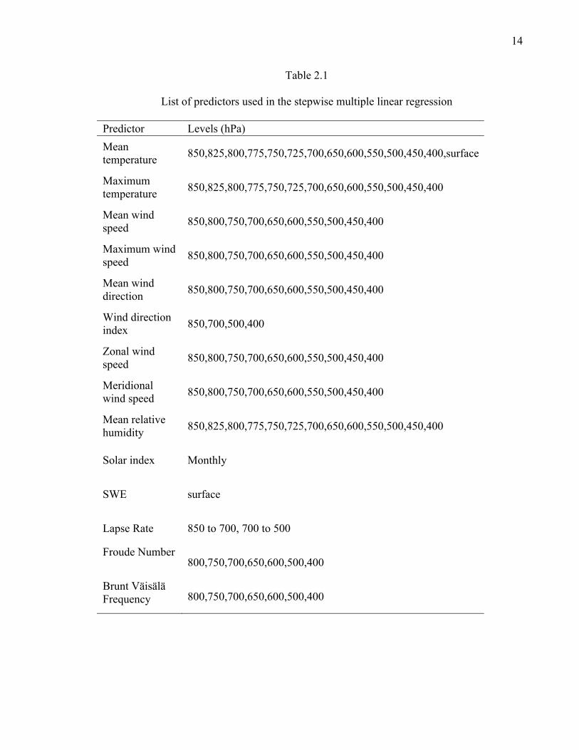
Table 2.1
List of predictors used in the stepwise multiple linear regression
Predictor Levels (hPa) Mean temperature 850,825,800,775,750,725,700,650,600,550,500,450,400,surface
Maximum temperature 850,825,800,775,750,725,700,650,600,550,500,450,400
Mean wind speed 850,800,750,700,650,600,550,500,450,400
Maximum wind speed 850,800,750,700,650,600,550,500,450,400
Mean wind direction 850,800,750,700,650,600,550,500,450,400
Wind direction index 850,700,500,400
Zonal wind speed 850,800,750,700,650,600,550,500,450,400
Meridional wind speed 850,800,750,700,650,600,550,500,450,400
Mean relative humidity 850,825,800,775,750,725,700,650,600,550,500,450,400
Solar index Monthly
SWE surface
Lapse Rate 850 to 700, 700 to 500
Froude Number 800,750,700,650,600,500,400
Brunt Väisälä Frequency 800,750,700,650,600,500,400

15
measure of QPF performance at Alta, we compare observed precipitation at CLN to NWS
15-39 h QPF (covering 1200 UTC to 1200 UTC and issued near 2100 UTC on the
previous day) from an archive of Graphical Forecast Editor (GFE) forecast grids. The
GFE forecasts over the Wasatch Mountains are based on a 2.5 km grid, with the grid box
of interest nearly centered over CLN and 65 m lower in elevation. At the time of writing,
there was only a short record of 2.5-km NWS QPF grids available for the Western
Region, covering a single winter season from Sep 2008 to Mar 2009.

CHAPTER 3
RESULTS
General SLR Characteristics at Alta
The mean SLR for the 457 snowfall events is 14.4, with a median of 13.3.
Grouping the data in bins of width 2 yields a mode between 10 and 12 (Fig. 3.1). Exact
10 SLR values occur in only 3% of events, in contrast to data from cooperative weather
observing sites, where the erroneous use of a 10 SLR to determine SWE without melting
a snow core is common (Baxter et al. 2005). The 25th and 75th percentile SLR values are
10 and 18, respectively. The mean SLR at CLN is lower than the 14.8 value obtained by
Roebber et al. (2003) for the NWS office in Salt Lake City (KSLC), with the SLR
distribution nearly identical to the Baxter et al. (2005) results for northern Utah. The
decrease in SLR from KSLC to CLN contrasts with the increase in SLR with increasing
elevation found by Grant and Rhea (1975). This difference, however, could be due to the
6-h resolution of snowfall measurements at NWS offices or differences in local wind
characteristics. SLR at CLN varies from 3.6 to 35.7, which is a smaller range than found
by Judson and Doesken (2000) and Roebber et al. (2003), who report on SLR at multiple
sites in the Rocky Mountains and contiguous United States, respectively. This result
might reflect our inclusion of only eight seasons of observations, and/or snow settlement
during the 1-12-h intervals between snow ending and measurement time.

17
Figure 3.1. Histogram of observed SLR values for all events.
18
Day-to-day SLR variability can be large. During a series of snowfall events
totaling 233 mm SWE from 3-12 Jan 2005, daily SLR ranged from 35.7 on the 6th to 5.2
on the 9th. Similarly, another storm cycle from 21-27 Nov 2001 (described in depth by
Steenburgh 2003) produced 210 mm SWE, with daily SLR values ranging from 7.1 to 23.
Sub-day SLR variability certainly exists, but is not captured by our dataset. For example,
an “average” 14.4 SLR event could consist of several hours of dendritic crystals, with
SLR possibly greater than 25, punctuated by periods of graupel, where SLR might be
much less than 10. Higher frequency measurements are needed to examine this
variability.
SLR varies considerably in all months, with the widest range of 3.6 to 35.1
occurring in February (Fig. 3.2). Mean and median monthly SLR are lowest in April
(12.3 and 11.6, respectively) and highest in March (15.6 and 14.1), although the medians
for months December through March are not significantly different at the 5% level.
There is a marked mid-winter peak in the number of extremely high SLR events.
Twenty-four of the 26 “wild snow” events (where SLR is 25 or more; Judson and
Doesken 2000) occur in December, January and February, with none observed in April.
The 26 wild snow events represent only 5.7% of the total, less than the 8% found
in the Park Range of Colorado (Judson and Doesken 2000). Nonetheless, wild snow
events at CLN include a 52 cm snowfall with an SLR of 27 on 5 Mar 2004. While the
data here are restricted to 1998 to 2007 to allow for inclusion of automated SWE
observations at CLN beginning in 1998, examination of the full CLN snowfall dataset
beginning Nov 1980 shows some other cases of wild snow worth noting, including 66 cm
of snow at an SLR of 41 on 7 Feb 1990. Wild snow events have the potential to yield

19
Figure 3.2. Box-and-whisker plot of SLR for all events. Box top and bottom represent the 75th and 25th percentiles, monthly median is indicated by a horizontal line, whiskers extend to the last outlier within 1.5 times the interquartile range, and additional outliers are indicated by ‘+’. Notches indicate statistical significance, where medians of two months are different at the 5% level when notches do not overlap.

20
large forecast errors when a fixed SLR value is applied and, although our sample size is
small in this regard, we will later attempt to identify specific factors favoring these
events.
On the low end of the SLR distribution, very heavy snow (SLR <= 5.5 as defined
by Dubé 2008) is observed in 12 (2.6%) of the events. Applying a fixed 10 or
climatological SLR in these events can lead to false alarms for NWS Winter Storm
Warning issuance. Although none of these events exceeded the 12- or 24-h Winter Storm
Warning criteria for the Wasatch Mountains, snowfall in half of these events would
exceed at least the 12-h warning criteria if the climatological mean SLR of 14.4 were
applied to the observed SWE. These events include 10 Jan 2005, where 52 mm SWE
yielded only 26.7 cm snowfall, corresponding to an SLR of 5.2. The full 1980-2007 CLN
snowfall dataset contains additional very heavy events, notably 11 Apr 1982, when 43.4
mm SWE and only 10.1 cm snow were recorded (an SLR of 2.3). Large variability in
SLR is clearly present at CLN, and the remainder of this study is concerned with
understanding and predicting this variability.
Relationships Between SLR and Local Atmospheric Conditions
Vertical Profiles
Evaluation of NARR thermal, moisture and wind profiles offers some insight into
relationships between meteorological conditions and SLR during storm events at CLN.
The strongest relationship is found between temperature and SLR, with the linear
correlation coefficient (R) largest at 650 hPa (R = −0.64; Fig. 3.3). For a subset of 80
high SWE (defined as > 25 mm) events (Fig. 3.4), the correlation is stronger (R = −0.76)

21
and peaks at 500 hPa. The near constant correlation coefficient magnitudes found for
temperatures at levels from 700 hPa up to 400 hPa contrast with Diamond and Lowry
(1954), who observed no relationship between snow density at the Central Sierra Snow
Laboratory and 500 hPa radiosonde temperatures, despite finding R = 0.64 at 700 hPa.
We attribute our findings at CLN to the typical thermal structure of Alta snowfall events,
where the mean 700 hPa to 500 hPa lapse rate is near moist adiabatic (6.6 K km-1) and is
non-negative in all 457 events, so that temperatures at and above 700 hPa are closely
related (e.g., R = 0.86 between 700 and 500 hPa temperatures).
The correlation between wind speed and SLR also peaks at 650 hPa for all events
(R = −0.39) and at 600 hPa for the high SWE subset (R = −0.64). The value of R between
relative humidity and SLR varies considerably with respect to pressure, but the
Figure 3.3. Vertical profiles of linear correlation coefficient between SLR and atmospheric variables for all events. Solid line, triangle markers, and dashed line indicate temperature, relative humidity and wind speed, respectively.
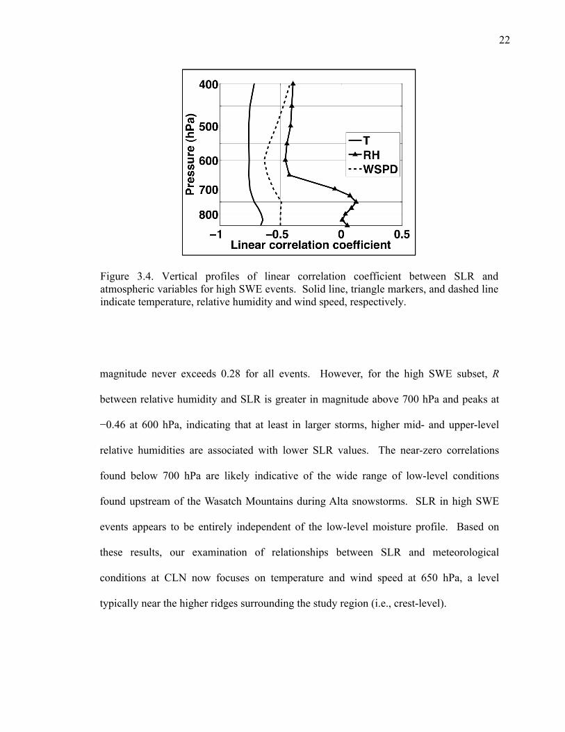
22
magnitude never exceeds 0.28 for all events. However, for the high SWE subset, R
between relative humidity and SLR is greater in magnitude above 700 hPa and peaks at
−0.46 at 600 hPa, indicating that at least in larger storms, higher mid- and upper-level
relative humidities are associated with lower SLR values. The near-zero correlations
found below 700 hPa are likely indicative of the wide range of low-level conditions
found upstream of the Wasatch Mountains during Alta snowstorms. SLR in high SWE
events appears to be entirely independent of the low-level moisture profile. Based on
these results, our examination of relationships between SLR and meteorological
conditions at CLN now focuses on temperature and wind speed at 650 hPa, a level
typically near the higher ridges surrounding the study region (i.e., crest-level).
Figure 3.4. Vertical profiles of linear correlation coefficient between SLR and atmospheric variables for high SWE events. Solid line, triangle markers, and dashed line indicate temperature, relative humidity and wind speed, respectively.

23
Near-Crest-Level Temperature
SLR shows an increase with increasing temperature from −23° to −17°C, and a
decrease with increasing temperature above −13°C (Fig. 3.5). The relationship is weak
near −15°C, where the highest SLR values occur and large scatter is present. We attribute
these result to the influence of temperature on crystal type, crystal size and riming. At
high supersaturations, when the temperature in a snow growth zone is close to −15°C, the
primary crystal form is dendritic, and ice crystal growth rates are at a local maximum
(Nakaya 1954). Operational forecasters typically define the “dendritic growth zone” as
the −12° to −18°C temperature range (e.g., BUFKIT; Mahoney and Niziol 1997). Wetzel
et al. (2004) suggest that temperatures near crest-level are likely to be close to the
temperatures of primary snow growth, where orographic upward vertical motions are
generally strong and thus high supersaturations are maintained. Therefore when
temperatures are within the −12° to −18°C range at 650 hPa, meteorological conditions
Figure 3.5. SLR versus 650-hPa temperature. Dashed line represents an SLR of 25.

24
favor the growth of large dendritic crystals having a high SLR. Observations by Power et
al. (1964) and Dubé (2008) suggest that SLR exceeds 25 almost exclusively with
dendritic crystals, and accordingly we find that 24 of the 26 wild snow events occur in
these conditions. Warmer or colder temperatures produce crystal types associated with
lower SLR, and yield slower crystal growth rates (Nakaya 1954; Dubé 2008). In
addition, Dubé (2008) notes that riming, having the potential to significantly reduce SLR,
is maximized at a temperature near −5°C, whereas the amount of supercooled water in a
cloud near −15°C is often too small for significant riming.
The decrease in SLR with decreasing temperature noted at the coldest
temperatures was observed by Grant and Rhea (1974), but most studies find a
homologous increase in SLR with decreasing temperature, although nonlinear and with
substantial scatter (e.g., LaChapelle 1962, Judson and Doesken 2000, Wetzel et al. 2004).
The trend observed here, which we attribute to a shift from dendritic to columnar crystals
near −18°C (Nakaya 1954) and reduced growth rates, might be missing from some
studies due to a small sample size at cold temperatures (e.g., Wetzel et al. 2004, where
there are no events included with temperatures below −18°C).
The greatest variability in SLR with respect to near-crest-level temperature occurs
close to −16°C, where SLR values from 8 to 35 are noted within a small range of
temperature. This range in SLR probably reflects a range in dendritic snow forms from
unaltered, mechanically aggregated snowflakes falling through a glaciated cloud in light
winds to rimed and heavily fragmented crystals falling through a mixed-phase cloud in
high winds. The dataset also likely contains events where snow growth takes place in
higher, colder clouds that produce columns or other crystal habits when near-crest-level

25
temperatures are within the dendritic growth zone.
Following Ware et al. (2006), the 457 snowfall events were divided at quintiles of
near-crest-level temperature (Fig. 3.6). The distribution for the lowest fifth of
temperatures (less than −15.1°C) has a mode near 17, and a long tail toward higher SLR
values. Fewer than 20% of these events have SLR values less than 15. For the highest
fifth of temperatures (greater than −7.9°C), no SLR values exceeding 20 are observed,
and 59% of these events have SLR values less than 10. Thus near-crest-level
temperatures alone provide a rough approximation for SLR and can be used in a
probabilistic sense to restrict the distribution of possible SLR values when temperatures
are very warm or cold.
Near-Crest-Level Wind Speed
SLR generally decreases with increasing 650-hPa wind speed, with R = −0.37 and
considerable scatter present at low speeds (Fig. 3.7). The trend is most pronounced above
10 m s-1, suggesting that 650-hPa free-air wind speeds of this magnitude are associated
with surface winds near CLN reaching a threshold for transport (Li and Pomeroy 1997,
Roebber et al. 2003). The greatest variability and highest values of SLR occur when
wind speeds are between 8 and 12 m s-1, with no wild snow events noted outside of this
range. Applying the Ware et al. (2006) approach here yields a clear shift in the SLR
distribution from the lowest to highest 650-hPa wind speeds (Fig. 3.8). For the lowest
quintile of 650-hPa wind speed (less than 8.1 m s-1), SLR values are distributed over a
wide range, with 27% of values exceeding 20. However, in the highest fifth (greater than
14.8 m s-1), 43% of events had an observed SLR of less than 10 (versus only 3% for the

26
Figure 3.6. Probability density function of the lowest and highest fifths of 650-hPa temperature.
Figure 3.7. SLR versus 650-hPa wind speed. Dashed line represents an SLR of 25.

27
Figure 3.8. Probability density function of the lowest and highest fifths of 650-hPa wind speed.
28
lowest fifth of wind speeds), and only 3% of values were above 20. High wind speeds
therefore suggest a low probability of high SLR, while wind speed has limited predictive
ability at low speeds.
SWE
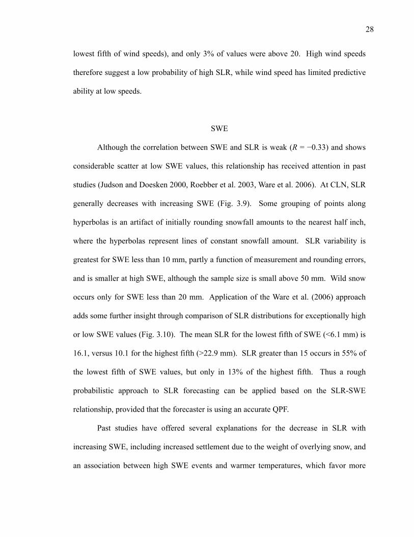
Although the correlation between SWE and SLR is weak (R = −0.33) and shows
considerable scatter at low SWE values, this relationship has received attention in past
studies (Judson and Doesken 2000, Roebber et al. 2003, Ware et al. 2006). At CLN, SLR
generally decreases with increasing SWE (Fig. 3.9). Some grouping of points along
hyperbolas is an artifact of initially rounding snowfall amounts to the nearest half inch,
where the hyperbolas represent lines of constant snowfall amount. SLR variability is
greatest for SWE less than 10 mm, partly a function of measurement and rounding errors,
and is smaller at high SWE, although the sample size is small above 50 mm. Wild snow
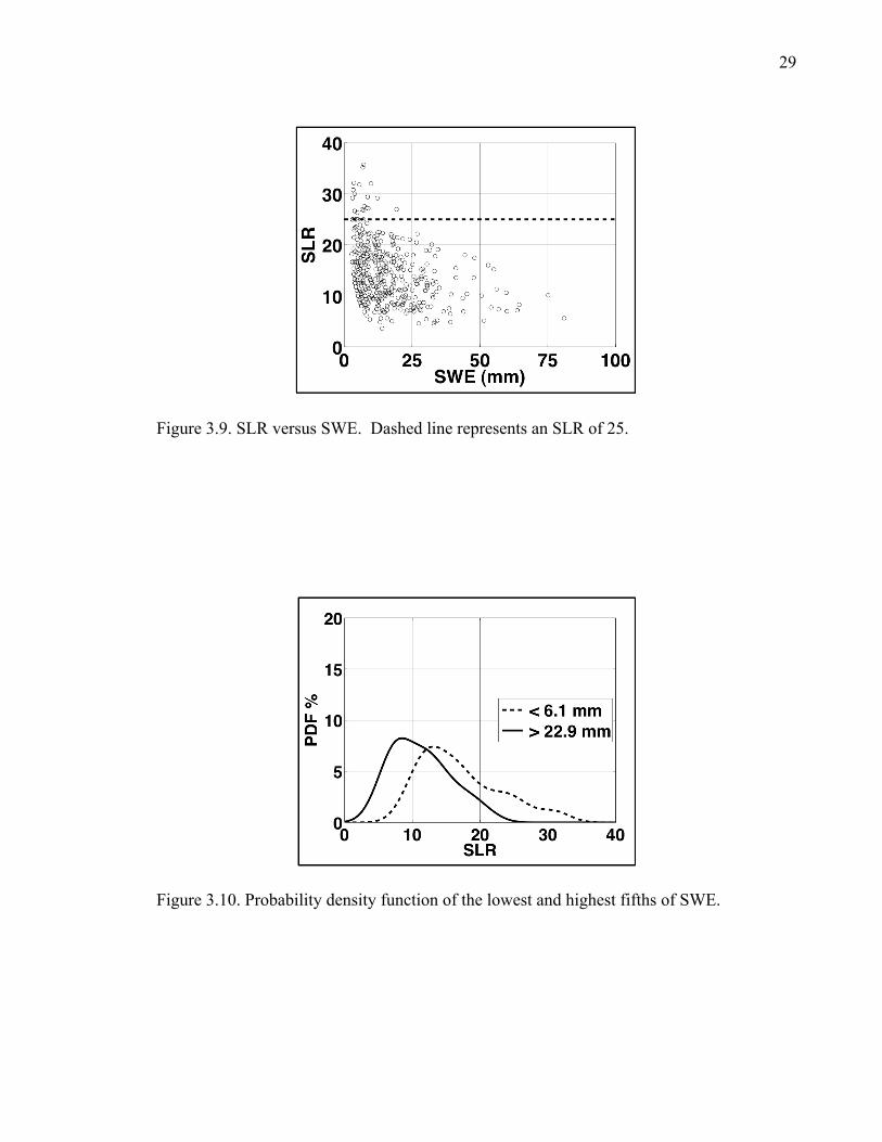
occurs only for SWE less than 20 mm. Application of the Ware et al. (2006) approach
adds some further insight through comparison of SLR distributions for exceptionally high
or low SWE values (Fig. 3.10). The mean SLR for the lowest fifth of SWE (<6.1 mm) is
16.1, versus 10.1 for the highest fifth (>22.9 mm). SLR greater than 15 occurs in 55% of
the lowest fifth of SWE values, but only in 13% of the highest fifth. Thus a rough
probabilistic approach to SLR forecasting can be applied based on the SLR-SWE
relationship, provided that the forecaster is using an accurate QPF.
Past studies have offered several explanations for the decrease in SLR with
increasing SWE, including increased settlement due to the weight of overlying snow, and
an association between high SWE events and warmer temperatures, which favor more
29
Figure 3.9. SLR versus SWE. Dashed line represents an SLR of 25.
Figure 3.10. Probability density function of the lowest and highest fifths of SWE.

30
riming and lower SLR crystal habits (Judson and Doesken 2000, Roebber et al. 2003).
The relationship between SWE and 650-hPa temperature at CLN is very weak (R = 0.16;
Fig. 3.11), but the highest SWE values tend to occur at temperatures above −12°C, where
riming is more likely and growth of lower-SLR plates and needles is favored. The
correlation between SWE and 650-hPa wind speed is stronger (R = 0.40; Fig. 3.12),
indicating that high SWE events are also characterized by higher wind speeds. High
wind speeds lead to snow transport and hence mechanical fragmentation, which decreases
SLR. Thus a portion of the SLR-SWE relationship likely comes about indirectly, due to
high SWE events being both warmer and windier.
Surface Temperature
The correlation between SLR and surface temperature (recorded at the CLN
observing site) is strong (R = −0.62) compared to that found for low-elevation sites in
other regions (e.g., Kyle and Wesley 1997). This result is due to close relationship
between free-air 650-hPa temperatures and temperatures at CLN (R = 0.93), an upper-
elevation site in terrain less prone to nocturnal and persistent cold pools than lowland
sites. Nevertheless, the effect of surface temperature at CLN is quite different from that
implied by the NWS MCT (Fig. 3.13). The MCT assigns SLR from 30 to 100 for surface
temperatures from −10° to −40°C, when SLR at CLN in fact averages 19.6 within this
temperature range, and exceeds 25 in only 9 of the 53 events (15%). The MCT also does
not assign SLR less than 10 to any temperature range, while these events represent 27%
of the total. The MCT is thus expected to have limited forecast value at CLN.

31
Figure 3.11. SWE versus 650 hPa temperature for all events.
Figure 3.12. SWE versus 650 hPa wind speed for all events.

32
Figure 3.13. Observed SLR and SLR indicated by the NWS MCT versus surface temperature for all events.

33
Other Processes
The wind direction and month indices, along with Froude number and the stability
parameters, individually explain less than 5% of the variance in SLR (R < 0.23; not
shown) for all events. For the high SWE subset, higher values of the wind direction
index at 700 hPa (i.e. greater deviation in flow direction from northwesterly) are weakly
related to lower SLR (R = −0.28; not shown). Although our primary focus is on the
atmospheric factors affecting SLR, there are other processes that must be considered.
Snow metamorphosis can reduce SLR in the hours between snowfall and measurement
(Doesken and Judson 1997). Judson and Doesken (2000) find snow density differences of
15% between cases where snowfall occurs during the last part of a measurement period
and snowfalls that occur throughout the measurement period. A similar effect is observed
at CLN, where the mean SLR is 14.2 when snow has been falling within 2 h of both
evening and morning measurement times, versus 13.8 when there has been no
precipitation during the 4 h prior to either measurement time.
Shortwave radiation effects are likely minimized at CLN due to the timing of
observations. Snow that falls during the day is typically exposed to limited solar
radiation due to associated cloud cover during the storm. Snow that falls at night is
measured before the sun rises (0400 LST). Nonetheless, snow that falls in the hours
immediately following morning measurement, followed by afternoon clearing, could
receive enough shortwave input to melt and decrease in depth, yielding an erroneously
low SLR. In December, mean SLR is 15.4 when snow falls within 3 h of evening
measurement, versus 14.9 when snow falls during the day and ceases more than 3 h prior
to evening measurement. In April, the decrease is greater, from 12.7 to 10.2, suggesting

34
that solar radiation does play a role.
Diagnosis and Prediction of SLR
Stepwise Multiple Linear Regression Using Reanalysis
The previous sections have discussed relationships between SLR and the thermal,
moisture, and wind profiles near CLN. We now estimate SLR using SMLR. Three types
of tests were performed to evaluate 1) the utility of the SMLR approach for explaining
the SLR variability for all events and high SWE events, 2) the sensitivity to the use of
predictors with large observational and forecast uncertainty, and 3) the sensitivity to the
use of hourly precipitation data. Absolute relative error (ARE), defined by
ARE =
€
xe − xoxo
3.1
and mean absolute relative error (MARE), defined by
MARE =
€
1n
xi,e − xi,oxi,o
∑ 3.2
where
€
n is the number of events,
€
xeand
€
xi,e represent the estimated or forecast value
and
€
xo and
€
xi,o the observed value (of the ith event for MARE), provide a more useful
quantification of fit quality in this situation than root-mean-square-error (RMSE). For
example, a 4.00 RMSE is more significant for an SLR of 10 than for 20, and thus implies
larger snowfall amount errors when computing QSF as the product of QPF and SLR.

35
Numerical results of the SMLR tests are shown in Table 3.1, where n denotes the number
of events in the subset, mean indicates whether predictors were calculated as a mean over
all 3-h periods of each event or only periods when at least 0.25 mm precipitation fell at
CLN, np is the number of predictors used in the regression equation, R is the linear
correlation coefficient, R2 is the coefficient of determination, RMSE is the root-mean-
square error, and MARE is the mean absolute relative error.
The purpose of test 1 was to determine the overall ability of SMLR to diagnose
SLR, and to evaluate whether the method is more effective for larger storms, during
which precipitation is less sporadic, and the range in SLR and the relative magnitude of
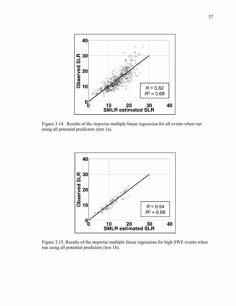
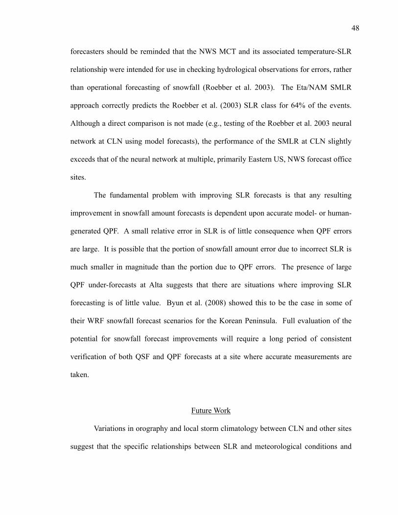
rounding and measurement errors are smaller. For all events, the stepwise tool uses 17
predictors to calculate a regression equation that yields R = 0.82 and a coefficient of
determination (R2 ) equal to 0.68 between estimated and observed SLR (Fig. 3.14). The
fit produces a mean absolute relative error (MARE) of 19%, which corresponds to a
range in estimated SLR of 12.2 to 17.9 for an observed SLR of 15.0. In another test of fit
quality, the regression estimate for 73% of events is within the correct Roebber et al.
(2003) SLR class.
The fit is much better for a high SWE (> 25 mm; n = 80) subset (Fig. 3.15), with
9 predictors producing R = 0.94, R2 = 0.88 and a MARE of 13%. This MARE
corresponds to an estimated SLR range of 13.1 to 17.0 for an observed SLR of 15.0.
Although the sample size is smaller, the SMLR approach is better able to diagnose SLR
during larger storms than for all events in the dataset, and models 83% of the events in
the correct Roebber et al. (2003) SLR class. Tables 3.2 and 3.3 list the predictors
included in the SMLR equations followed by cumulative variance explained (R2 between

36
Table 3.1
Results of the stepwise multiple linear regression
Test SWE n Predictors Mean np R R2 RMSE MARE
1a >= 2.8 mm 457 All During
precip 17 0.82 0.68 3.34 0.19
1b >= 25.4 mm 80 All During
precip 9 0.94 0.88 1.60 0.13
2a >= 2.8 mm 457 T only During
precip 6 0.73 0.53 3.99 0.24
2b >= 2.8 mm 457 T, wind During
precip 11 0.79 0.63 3.56 0.20
2c >= 25.4 mm 80 T only During
precip 3 0.80 0.63 2.65 0.21
2d >= 25.4 mm 80 T, wind During
precip 5 0.91 0.83 1.84 0.14
3a >= 2.8 mm 457 T, wind All
periods 12 0.78 0.60 3.69 0.21
3b >= 2.8 mm 457 All All
periods 16 0.81 0.65 3.49 0.20
3c >= 25.4 mm 80 T, wind All
periods 8 0.90 0.82 1.86 0.14
3d >= 25.4 mm 80 All All
periods 7 0.92 0.85 1.71 0.13
37
Figure 3.14. Results of the stepwise multiple linear regression for all events when run using all potential predictors (test 1a).
Figure 3.15. Results of the stepwise multiple linear regression for high SWE events when run using all potential predictors (test 1b).

38
Table 3.2
Predictors included in the SMLR equations for test 1a
Predictor Cumulative Variance Explained T650 0.404
WSPD600^2 0.475 SWE 0.517 V400 0.549
T600^3 0.585 T800^3 0.602 T600 0.616
RH550 0.624 RH725 0.630 RH850 0.647 DIR700 0.650
WINDEX700 0.656 T500^2 0.659 T500^3 0.666 T550^3 0.671
MAXSPD400 0.675 WSPD600 0.678
Table 3.3
Predictors included in the SMLR equations for test 1b
Predictor Cumulative Variance Explained T550 0.506
WSPD600^2 0.656 T775 0.739 V650 0.801 T400 0.821
T850^(-1) 0.844 WINDEX850 0.853
RH450^3 0.866 RH825^3 0.877

39
observed SLR and the regression estimate), for all events and the high SWE subset,
respectively, where T, WSPD, MAXSPD, U, V, RH, DIR and WINDEX represent
temperature, wind speed, maximum wind speed, zonal wind speed, meridional wind
speed, relative humidity, wind direction and wind direction index at the given pressure
level (hPa).. The final values of R2 are much higher than those achieved using any single
variable in this study or in past studies by Diamond and Lowry (1954), Judson and
Doesken (2000), Wetzel et al. (2004) and Simeral (2005).
In test 2, we investigate whether eliminating poorly-resolved or forecasted
variables (e.g., relative humidity) from the set of possible predictors has a significant
negative effect on our results. Reducing the field of predictors to temperature, wind
direction and wind speed yields a fit with R2 = 0.63 for all events (Fig. 3.16), and R2 =
0.83 for high SWE events (Fig. 3.17). In both tests, MARE only increases by a few
percent. Thus there is not a large reduction in fit quality when limiting predictors to those
that are better known. In a further test (not shown), a fit using temperature predictors
alone explains 53% of the variance in SLR for all events, and 63% for high SWE events.
Up to this point, predictors have been calculated as a mean during only 3-h
periods when at least 0.25 mm of precipitation was recorded by the automated gauge at
CLN. However, to forecast SLR by this method would require an accurate QPF
distribution. Additionally, Eta/NAM forecasts tested in the next section are 6-hourly and
produce 40-km grid QPF that has almost no relationship to SWE observed at CLN. A
second option exists, where predictors are instead calculated as a mean of all periods,
with no regard for the temporal distribution of precipitation. Calculating inputs as a 24-h
mean reduces R2 from 0.68 to 0.65 for all events, and from 0.88 to 0.85 when all

40
Figure 3.16. Results of the stepwise multiple linear regression for all events when run using only temperature and wind predictors (test 2b).
Figure 3.17. Results of the stepwise multiple linear regression for high SWE events when run using only temperature and wind predictors (test 2d).

41
predictors are included (tests 3a-b; estimated versus observed SLR not shown). A similar
reduction in R2 occurs using only temperature and wind predictors, with the regression
equation still producing 0.60 and 0.82 for all events and the high SWE subset,
respectively (tests 3c-d; not shown). Thus, when large uncertainty exists regarding the
amount and temporal distribution of precipitation, it is still possible to explain 60% to
85% of the variance in SLR at CLN using only 24-h mean reanalysis temperature and
wind inputs.
Application to Eta/NAM Forecasts
The tests above involve the use of reanalysis data, and are therefore not a true
assessment of forecast skill, which requires the use of forecast variables to predict SLR.
NARR biases differ from those in operational models, and our application of a “perfect
prog” technique (described by Glahn and Lowry 1972) in the previous section involves
developing a regression equation and testing it on the same set of events. In order to test
the ability of an operational model to predict SLR, we ran SMLR on a dependent set of
events using predictors from the Eta/NAM model, then tested the resulting regression
equation on an independent set of events. For this test, the total number of events was
reduced to 356 (78% of the original dataset), due to gaps in the NCAR Eta/NAM archive.
These events were randomly split into a dependent set of 180 events and an independent
set of 176 events. Six predictors were selected using the same criteria as for the NARR
tests (0.05 entrance tolerance, 0.10 exit tolerance): temperature at 750, 700, 650 and 600
hPa, 550-hPa meridional wind speed, and maximum 650-hPa wind speed, which fit the
dependent set with R2 = 0.58 (not shown). When applied to the independent set, R2

42
between the predicted and observed SLR was 0.51 (Fig. 3.18). The MARE was 25%,
equivalent to a forecast range of 11.3 to 18.8 for an observed SLR value of 15. ARE
exceeded 50% in less than 12% of events. The algorithm was able to predict the correct
category of SLR (based on the Roebber et al. 2003 divisions; section 2c) in 63% of the
forecast cases. A Monte Carlo simulation using 1000 unique selections of independent
and dependent sets yielded median and standard deviation R2 values of 0.48 and 0.04,
respectively, indicating that the performance of SMLR in the aforementioned test reflects
typical results, and that the process is not overly sensitive to the specific choice of events
included in the two sets.
The SMLR approach offers considerable improvement over some existing
techniques. Applying a climatological SLR value to the independent set yields a MARE
of 0.45, nearly double that of the MOS. ARE for the climatological SLR exceeds 50% in
28% of the forecast cases. Testing of the predictive ability of the NWS MCT is
somewhat difficult due to the lack of an accurate Eta/NAM 2-m surface temperature for
CLN (since the nearest grid point is at a much lower elevation). The MCT was instead
tested using 700-hPa temperature as an approximation for CLN surface temperature,
noting that RMSE = 1.0°C between NARR 700-hPa temperature and observed surface
temperature. The MCT consistently overpredicts SLR, with a MARE of 99% and ARE
values exceeding 50% in more than half of the forecast events.
A caveat to improving SLR prediction is that snowfall forecasting remains a
three-step process. An accurate forecast of snowfall amount, and hence improved skill in
warning issuance, relies on accurate prediction of both QPF and SLR. Assessment of any
potential benefit of the SMLR approach to point-specific snowfall forecasting requires

43
0 10 20 30 400
10
20
30
40
Forecast SLR
Ob
served
SL
R
FIG. 12. Observed versus Eta MOS forecast SLR
for an independent set of 177 events, using only
temperature and wind predictors.
R = 0.71
R2 = 0.51
Figure 3.18. Observed versus forecast SLR for an independent set of 176 events, using Eta/NAM temperature and wind predictors.

44
some sense of QPF skill in LCC. The linear correlation coefficient between NWS Alta
grid point QPF and observed precipitation is 0.76 for the period of record sampled (Sep
2008 to Mar 2009; Fig. 3.19). ARE in QPF can be large, showing difficulties with both
under- and over-forecasting. The largest relative errors result from under-forecasts,
including a forecast of 13 mm when 47 mm was observed, and two forecasts of 3 mm
when 19 mm was observed. In these cases and others where large QPF errors occur, it is
unlikely that any refinement of the SLR forecast technique could lead to improved
prediction of snowfall amount. However, relative errors for the four highest QPF values
were all less than 20%, and in these cases and others where QPF is skillful, improving the
final step of the snowfall forecast process beyond using a fixed climatological SLR or an
incorrect empirical relationship is clearly a worthwhile endeavor.

45
0 10 20 30 40 500
10
20
30
40
50
NWS Alta grid point QPF (mm)
CL
N o
bserv
ed
pre
cip
itati
on
(m
m)
R = 0.76
R2 = 0.58
FIG. 13. Precipitation observed at CLN versus
NWS Alta grid point QPF for Sept 2008 to Mar
2009.
Figure 3.19. Observed precipitation versus NWS Alta grid point QPF.

CHAPTER 4
CONCLUSIONS
Summary
We have investigated the variability of SLR at a high-mountain site where winter
storms are frequent, the effects of sun, wind transport and ground temperature are
reduced, and measurement practices are reliable and consistent. The mean SLR of 14.4 is
similar to that found for nearby lowland sites, and large SLR variability is found during
all months under study. Wild snow events (where SLR > 25) comprise only 5.7% of the
events in this study, but can be associated with large snowfall amount errors. Our
analysis provides information regarding the relationship between SLR and
meteorological conditions at CLN:
1) SLR is correlated with crest-level temperature and wind speed, particularly for
high SWE events, and weakly correlated with SWE, relative humidity, Froude
number, stability, wind direction and time-of-year.
2) SLR decreases (increases) with increasing near-crest-level temperature above
(below) −15°C, which we attribute to changes in crystal type and size, and
increased frequency and intensity of riming at warmer temperatures.
3) SLR decreases with increasing near-crest-level wind speed above 10 m s-1, an
approximate threshold for snow transport.

47
4) SLR decreases with increasing SWE, although the relationship is weak. Higher
SWE at CLN is associated with warmer crest-level temperatures and higher wind
speeds.
5) Most wild snow events occur within three ranges of conditions: i) 650 hPa
temperatures between −18° and −12°C, ii) 650 hPa winds between 8 and 12 m s-1,
and iii) SWE less than 20 mm.
Combining several variables, the stepwise multiple linear regression approach is able
to explain 68% of the variance in SLR for all 457 snowfall events. While we are able to
diagnose to a great extent the conditions affecting SLR at CLN, we are still unable to
explain a sizable portion of the variance. This portion of the variability could stem from
a variety of sources, from our failure to entirely capture the non-linear relationships
between selected predictors and SLR to unresolved physical processes, observational
errors, low temporal resolution of measurements and high temporal variability in
atmospheric conditions. Although our results could be affected by a small sample size (n
= 80), the skill of the stepwise approach is greater for larger events, explaining 88% of
the variance in SLR for a high SWE (> 25 mm) subset. The ability of the regression
approach to diagnose SLR is not greatly reduced by restricting predictors to only
temperature and wind, or by ignoring the temporal distribution of precipitation and
calculating predictors as a 24-h mean.
The SMLR forecast algorithm is able to predict SLR for an independent set of
events with much greater skill than using a fixed ratio or using the NWS MCT. The MCT
produced large errors in SLR for many of the independent forecast cases and a MARE of
99%, equivalent to an SLR forecast range of 10.1 to 40.0 when 20.1 is observed. Thus
48
forecasters should be reminded that the NWS MCT and its associated temperature-SLR
relationship were intended for use in checking hydrological observations for errors, rather
than operational forecasting of snowfall (Roebber et al. 2003). The Eta/NAM SMLR
approach correctly predicts the Roebber et al. (2003) SLR class for 64% of the events.
Although a direct comparison is not made (e.g., testing of the Roebber et al. 2003 neural
network at CLN using model forecasts), the performance of the SMLR at CLN slightly
exceeds that of the neural network at multiple, primarily Eastern US, NWS forecast office
sites.
The fundamental problem with improving SLR forecasts is that any resulting
improvement in snowfall amount forecasts is dependent upon accurate model- or human-
generated QPF. A small relative error in SLR is of little consequence when QPF errors
are large. It is possible that the portion of snowfall amount error due to incorrect SLR is
much smaller in magnitude than the portion due to QPF errors. The presence of large
QPF under-forecasts at Alta suggests that there are situations where improving SLR
forecasting is of little value. Byun et al. (2008) showed this to be the case in some of
their WRF snowfall forecast scenarios for the Korean Peninsula. Full evaluation of the
potential for snowfall forecast improvements will require a long period of consistent
verification of both QSF and QPF forecasts at a site where accurate measurements are
taken.
Future Work
Variations in orography and local storm climatology between CLN and other sites
suggest that the specific relationships between SLR and meteorological conditions and

49
the SMLR results presented in this manuscript might not be directly applicable to other
sites across the United States or even in the Intermountain region. However, the
approach described herein serves as proof of concept for the use of a straightforward
regression method that could be incorporated into existing guidance products, with the
goal of improving the snowfall amount forecast process. In addition, while skill in
snowfall amount forecasts ultimately relies on accurate QPF, the forecasts of SLR alone
are useful for avalanche forecasting and hydrological applications.
Future work will involve further investigation of wild snow events, due to the
high potential for snowfall forecast busts in these situations. The algorithm described in
this manuscript will be incorporated into forecast operations at the National Weather
Service in Salt Lake City and potentially at the Utah Traffic Operations Center. The
algorithm will be evaluated at several sites in northern Utah, and a separate regression
equation will likely be determined for the Salt Lake City airport.

REFERENCES
Abbe, C., 1888: Appendix 46. 1887 Annual report of the Chief Signal Officer of the Army under the direction of Brigadier-General A. W. Greely, U.S. Govt. Printing Office, Washington, DC, 385-386.
Baxter, M. A., C. E. Graves, and J. T. Moore, 2005: A climatology of snow-to-liquid
ratio for the contiguous United States. Wea. Forecasting, 20, 729-744. Bourgouin, P., 2000: A method to determine precipitation types. Wea. Forecasting, 15,
583–592. Bossolasco, M., 1954: Newly fallen snow and air temperature. Nature, 174, 362-363. Byun, K.-Y., J. Yang, and T.-Y. Lee, 2008: A snow-ratio equation and its application to
numerical weather prediction. Wea. Forecasting, 23, 644-658. Casson, J., M. Stoelinga, and J. Locatelli, 2008: Evaluating the importance of crystal type
on new snow instability: a strength vs. stress approach using the SNOSS model. Proceedings of the International Snow Science Workshop, Whistler, B. C., CD-ROM.
Cobb, D. K., and J. S. Waldstreicher, 2005: A simple physically based snowfall
algorithm. Preprints, 21st Conf. on Weather Analysis and Forecasting and 17th Conf. on Numerical Weather Prediction, Washington, DC, Amer. Meteor. Soc., CD-ROM, 2A.2.
Cosgrove, R. L., and B. S. Sfanos, 2004: Producing MOS snowfall amount forecasts from
cooperative observer reports. Preprints 20th Conference on Weather Analysis and Forecasting, Seattle, Amer. Meteor. Soc.
Dallavalle, J. P., M. C. Erickson, and J. C. Maloney, 2004: Model Output Statistics
(MOS) Guidance for Short-Range Projections. Preprints, 20th Conference on Weather Analysis and Forecasting, Seattle, Amer. Meteor. Soc.
Diamond, M., and W. P. Lowry, 1954: Correlation of density of new snow with 700-
millibar temperature. J. Meteor., 11, 512-513.
51
Doesken, N. J., and A. Judson, 1997: The Snow Booklet: A guide to the science, climatology, and measurement of snow in the United States. Dept. of Atmospheric Science, Colorado State University, 86 pp.
Dubé, I., cited 2008: From mm to cm…: Study of snow/liquid water ratios in Quebec.
Meteorological Service of Canada, Quebec, QC, Canada. [Available online at http://www.meted.ucar.edu/norlat/snowdensity/from_mm_to_cm.pdf.]
Dunn, L. B., 1983: Quantitative and spatial distribution of winter precipitation along
Utah’s Wasatch Front. NOAA Tech. Memo. NWS WR-181, 71 pp. [Available from National Weather Service Western Region, P.O. Box 11188, Salt Lake City, UT 84147-0188.]
Glahn, H.R., and D.A. Lowry, 1972: The use of model output statistics (MOS) in
objective weather forecasting. J. Appl. Meteor., 11, 1203–1211. Grant L. O., and J. O. Rhea, 1974: Elevation and meteorological controls of the density
of snow. Proc. Advanced Concepts Tech. Study Snow Ice Resources Interdisciplinary Symp., National Academy of Science, 169–181.
Gunn, K. L. S., 1965: Measurements on new-fallen snow. McGill University Stormy
Weather Group Scientific Report MW-44. Prepared for United States Air Force, Contract No. AF19(628)-249. Bedford, Massachusetts, 27 pp.
Hart, K.A., W.J. Steenburgh, and D.J. Onton, 2005: Model forecast improvements with
decreased horizontal grid spacing over finescale Intermountain orography during the 2002 Olympic Winter Games. Wea. Forecasting, 20, 558–576.
Judson, A., and N. Doesken, 2000: Density of freshly fallen snow in the central Rocky
Mountains. Bull. Amer. Meteor. Soc., 81, 1577-1587. Kyle, J. P., and D. A. Wesley, 1997: New conversion table for snowfall to estimated
meltwater: Is it appropriate in the High Plains? Central Region ARP 18-04, National Weather Service, Cheyenne, WY, 4 pp.
LaChapelle E. R., 1962: The density distribution of new snow. Project F, Progress Rep.
2, USDA Forest Service, Wasatch National Forest, Alta Avalanche Study Center, Salt Lake City, UT, 13 pp.
——, 1980: The fundamental processes in conventional avalanche forecasting. J.
Glaciology, 26, 75-84. Li, L., and J. W. Pomeroy, 1997: Estimates of threshold wind speeds for snow transport
using meteorological data. J. Appl. Meteor., 36, 205-213. Mahoney, E. A., and T. A. Niziol, 1997: BUFKIT: A software application toolkit for

52
predicting lake-effect snow. Preprints, 13th Intl. Conf. on Interactive Information and Processing Systems for Meteorology, Oceanography, and Hydrology, Long Beach, CA, Amer. Meteor. Soc., 388-391.
Marwitz, J., 1987: Deep orographic storms over the Sierra Nevada. Part I:
Thermodynamics and kinematic structure. J. Atmos. Sci., 44, 159-173.J. Atmos. Sci., 56, 3573-3592.
McNeally, P.B., 2000: Avalanche Stability Modeling using GIS, M.S. thesis, University
of Utah, 120 pp. Mesinger, F., G. DiMego, E. Kalnay, K. Mitchell, P.C. Shafran, W. Ebisuzaki, D. Jović,
J. Woollen, E. Rogers, E.H. Berbery, M.B. Ek, Y. Fan, R. Grumbine, W. Higgins, H. Li, Y. Lin, G. Manikin, D. Parrish, and W. Shi, 2006: North American Regional Reanalysis. Bull. Amer. Meteor. Soc., 87, 343–360.
Nakaya, U., 1954: Snow Crystals, Natural and Artificial. Harvard University Press, 510
pp. Power, B. A., P. Summers, and J. D'Avignon, 1964: Snow crystal forms and riming
effects as related to snowfall density and general storm conditions. J. Atmos. Sci., 21, 300-305.
Roebber, P.J., S.L. Bruening, D.M. Schultz, and J.V. Cortinas, 2003: Improving snowfall
forecasting by diagnosing snow density. Wea. Forecasting, 18, 264–287. ——, M.R. Butt, S.J. Reinke, and T.J. Grafenauer, 2007: Real-time forecasting of
snowfall using a neural network. Wea. Forecasting, 22, 676–684. Simeral, D. B., 2005: New snow density across an elevation gradient in the Park Range
of northwestern Colorado, M. A. thesis, Northern Arizona University, 101 pp. Steenburgh, W. J., 2003: One hundred inches in one hundred hours: evolution of a
Wasatch Mountain Winter storm cycle, Wea. Forecasting, 18, 1018-1036. ——, and T. I. Alcott, 2008: Secrets of the “Greatest Snow on Earth.” Bull. Amer.
Meteor. Soc., 89, 1285-1293. U.S. Department of Commerce, 1996: Supplemental observations. Part IV, National
Weather Service Observing Handbook No. 7: Surface Weather Observations and Reports, National Weather Service, Silver Spring, MD, 57 pp.
UDOT-District Two, 1987: Snow avalanche atlas: Little Cottonwood Canyon—U210,
UDOT, 81 pp.
53
Ware, E. C., D. M. Schultz, H. E. Brooks, P. J. Roebber, and S. L. Bruening, 2006: Improving snowfall forecasting by accounting for the climatological variability of snow density. Wea. Forecasting, 21, 94–103.
Wetzel, M., M. Meyers, R. Borys, R. McAnelly, W. Cotton, A. Rossi, P. Frisbie, D.
Nadler, D. Lowenthal, S. Cohn, and W. Brown, 2004: Mesoscale snowfall prediction and verification in mountainous terrain. Wea. Forecasting, 19, 806–828.
Yang, D., et al., 1998: Accuracy of NWS standard 8” nonrecording precipitation gauge:
Results and application of WMO intercomparison. J. Atmos. Oceanic Technol., 15, 54-68.