smp workshop on cavitation and propeller performances: the ... · second international symposium on...

Second International Symposium on Marine Propulsors smp’11, Hamburg, Germany, June 2011

Workshop: Propeller performance

SMP Workshop on Cavitation and Propeller Performances: The Experience of the University of Genova on the Potsdam Propeller Test

Case

Stefano Gaggero1, Diego Villa

1, Stefano Brizzolara

1

1University of Genova, Department of Naval Architecture, Marine and Electrical Engineering, Genoa, Italy

ABSTRACT

Accurate and reliable propeller performances predictions

are a fundamental aspect for any analysis and design of a

modern propeller. Prediction of cavitation and cavity

extension is another important task, being cavitation one

of the crucial aspects that influences efficiency in addition

to propagated noise and blade vibration and erosion.

Accurate prediction of induced velocity field downward

the propeller plane is, moreover, mandatory for the proper

design of appendages and rudders. The Potsdam Propeller

Test Case within the SMP Workshop on Cavitation and

Propeller Performances represents an excellent chance to

test and to validate the capabilities of the University of

Genova, together with its numerical tools, in predicting

propeller open water performances and cavitation.

Keywords

CFD, Panel Method, Cavitation, Propeller Performances.

1 INTRODUCTION

The design and the analysis of modern, loaded and highly

skewed propellers is a primary aspect in the naval

architecture field. The growing demand of heavily loaded,

highly efficient propeller with request of very low noise

and vibration levels onboard makes the design of marine

propellers more and more conditioned by the analysis of

inception and developed cavitation. Cavitation, in fact, is

the more important inhibitor to the propulsion system. If

not specifically scheduled, as in the case of

supercavitating propellers, cavitation can generate a

number of problems, like additional noise, vibrations and

erosions as well as variations in the developed thrust and

torque. Moreover, on modern propellers design, midchord

bubble cavitation may also appears and face cavitation is

very common, especially if the propeller operates behind

a strong nonuniform wake or in inclined shaft conditions.

Propeller performances, in addition, affect the efficient

design of rudders and appendages that have to operate,

hopefully in cavity free conditions, inside the wake field

behind the propeller itself. The prediction of the

downstream velocity distribution produced by the

propulsor, with special attention to the developed tip

vortex, is, as a consequence, another crucial aspect for an

accurate and useful analysis.

From a numerical point of view it is comprehensive the

need of both accurate and efficient solvers, able to address

the problem of performances and cavitation prediction in

the preliminary design stage and in the more accurate

final propeller optimization phase, during which features

like tip vortex detachment or cavity bubble dynamics are

taken into account. While in daily practice design

boundary elements methods are usually applied because

of their extreme computationally efficiency and their

overall accuracy in both non cavitating and cavitating

conditions for an acceptable range of advance coefficient

around the design point, the increase in hardware

resources leads to a shift towards viscous solvers for a

more detailed propeller analysis. Major advantages of

these approaches include the modeling accuracy, the

amount of detailed information extracted from the

simulations and the possibility of full scale analysis.

The Potsdam Propeller Test Case within the SMP

Workshop on Cavitation and Propeller Performances

represents an excellent chance to test and to validate the

capabilities of the University of Genova, together with its

numerical tools, in predicting propeller open water

performances and cavitation. In particular two different

approaches and three different solvers have been applied

for the computation of open water propeller performances

and cavitation prediction. The first approach is a potential

based boundary element method developed at the

University of Genova by Gaggero (2010), widely

validated in steady and unsteady conditions

(Gaggero, 2008, 2010), including also cavitation. This

approach will be adopted for the prediction only of the

Potsdam Propeller open water curves and of the cavity

extension. The approximate hypothesis on which the

solver is based, in fact, does not make it suitable for a

reliable prediction of the induced velocities and tip

vortex, especially close to the mathematically “singular”

trailing vortical wake, where a complex viscous

interaction takes place. The second approach is based on

the solutions of Reynolds Averaged Navier-Stokes

equations through two different solvers. In the first case a

commercial RANS solver, StarCCM+ v. 5.06 (CD-

Adapco, 2010), has been applied for all the required

computations: open water performances prediction,

evaluation of downstream velocities and cavity extension.

In the second case the open source CFD package

OpenFOAM (OpenCFD, 2010) has been adopted for the

computation, due to computational an time resources

limitations, only of propeller open water characteristics.

2 NUMERICAL SOLVERS

2.1 Panel Method

Panel/boundary elements methods model the flowfield

around a solid body by means of a scalar function, the

perturbation potential ( ), whose spatial derivatives

represent the component of the perturbation velocity

vector. Irrotationality, incompressibility an absence of

viscosity are the hypothesis needed in order to write the

more general continuity and momentum equations as a

Laplace equation for the perturbation potential itself:

( ) (1)

For the more general problem of cavitating flow, Green‟s

third identity allows to solve the three dimensional

differential problem as a simpler integral problem written

for the surfaces that bound the domain. The solution is

found as the intensity of a series of mathematical

singularities (sources and dipoles) whose superposition

models the inviscid cavitating flow on and around the

body.

( ) ∫ ( )

∫ ( )

∫ ( )

(2)

Neglecting the supercavitating case (computation is

stopped when the cavity bubble reaches the blade trailing

edge) and assuming that the cavity bubble thickness is

small with respect to the profile chord, (Gaggero, 2009)

singularities that model cavity bubble can be placed on

the blade surface instead than on the real cavity surface,

leading to an integral equation in which the subscript q

corresponds to the variable point in the integration, n is

the unit normal to the boundary surfaces and rpq is the

distance between points p and q, SB is the fully wetted

surface, SW is the wake surface and SCB is the projected

cavitating surface on the solid boundaries. This approach

can be addressed as a partial nonlinear approach that takes

into account the weakly nonlinearity of the boundary

conditions (the dynamic boundary condition on the

cavitating part of the blade and the closure condition at its

trailing edge) without the need to collocate the

singularities on the effective cavity surface. The set of

required boundary conditions for the steady problem is:

Kinematic boundary condition on the wetted solid

boundaries:

( )

( ) (3)

Kutta condition at blade trailing edge:

( ) ( )

( ) (4)

Dynamic boundary condition on the cavitating

surfaces:

(5)

Kinematic boundary condition on the cavitating

surfaces (where n is the normal vector and th is the

local cavity bubble thickness):

( ) ( ) (6)

Cavity closure condition at cavity bubble trailing

edge.

Arbitrary detachment line, on the back and/or on the face

sides of the blade can be found, iteratively, applying a

criteria equivalent, in two dimensions, to the Villat-

Brillouin cavity detachment condition, as in Mueller

(1999). Starting from a detachment line obtained from the

initial wetted solution (and identified as the line that

separates zones with pressures higher than the vapor

tension from zones subjected to pressure equal or lower

pressures) or an imposed one (typically the leading edge),

the detachment line is iteratively moved according to:

If the cavity at that position has negative thickness, the

detachment location is moved toward the trailing edge

of the blade.

If the pressure at a position upstream the actual

detachment line is below vapor pressure, then the

detachment location is moved toward the leading edge

of the blade.

The numerical solution consists in an iterative scheme

delegated to solve the nonlinearities connected with the

Kutta, the dynamic and the kinematic boundary

conditions on the unknown cavity surfaces until the cavity

closure condition has been satisfied. Viscous forces,

neglected by the potential approach, can be computed

following two different approaches. In the first case, as

proposed by Hufford (1992) and Gaggero (2010), a thin

boundary layer solver can be coupled, through

transpiration velocities, to the inviscid solution, in order

to obtain a local estimation of the frictional coefficient

computed in accordance to the integral approach of Curle

(1967) (for the laminar boundary layer) and Nash (1969)

(for the turbulent boundary layer). This approach, though

being applied successfully for the analysis of

conventional propellers, poses some problems of

convergence in very off design conditions and suffers

from the tip influence on streamlines on which the

boundary layer calculation is performed. As a

consequence in the present work a local estimation of

frictional coefficient has been carried out applying a

standard frictional line. In particular, the VanOossanen

formulation, based on local chord and thickness/chord

ratio, has been employed:

( )

(

( )

( ))

( ) (7)

A further force free condition for the trailing vortical

wake can be employed, at least for the steady

computations, requiring that each points move, from a

Lagrange point of view, following:

( ̂) ( ̂ ) ( ) ̂ (8)

Figure 1: Panel Method propeller surface mesh.

In present work, however, only an approximate

description of the trailing vortical wake dynamics has

been adopted, and the trailing vortical wake has been

modeled as a steady helicoidal surface whose pitch equals

the local blade pitch.

The discretized surface mesh consists of 2500

hyperboloidal panels for each blade. The trailing vortical

wake extends for five complete revolutions and it is

discretized with a time equivalent angular step of 6°, as in

figure 1.

2.2 RANS Solver – StarCCM+ and OpenFOAM

Analysis of open water propeller characteristics has been

carried out through StarCCM+, a commercial finite

volume RANS solver and by OpenFOAM, an open source

CFD package. Continuity and momentum equation, for an

incompressible flow, are expressed by:

{ ̇

(9)

in which is the averaged velocity vector, is the

averaged pressure field, is the dynamic viscosity, is

the momentum sources vector and is the tensor of

Reynold stresses. Cavitation is computed using a volume

of fluid approach for the vapor fraction inside the domain,

thus requiring the solution of a further transport equation

for the percentage of vapor inside each cell. The bubble

growth rate is based on the extended Rayleigh-Plesset

equation (CD-Adapco, 2010).

Two turbulence closure equations models have been

selected within StarCCM+. The and the

models have been adopted for the computation of

open water and induced velocity propeller characteristics,

in order to investigate the influence of the turbulence

model on the non cavitating solution. For the

computations in cavitating regime, only the more stable

has been applied. OpenFOAM

computations, instead, have been carried out adopting

only the closure equations.

The StarCCM+ computational domain, by means of the

symmetries, is represented by an angular sector of

amplitude ⁄ around a single blade, discretized with

unstructured meshes of polyhedral cells. OpenFOAM

domain, due to the selected simulation model, instead is

represented by a cylindrical region surrounding the entire

propeller, discretized also in this case, using polyhedral

elements. All the simulations, for both the solvers, have

been carried out as steady, using the Moving Reference

Frame approach. SIMPLE algorithm links pressure with

velocity fields.

Figure 2: Typical unstructured Mesh for Open Water

Computations. 1.25M/blade.

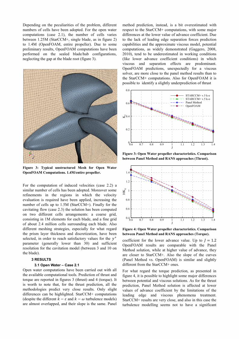
Depending on the peculiarities of the problem, different

numbers of cells have been adopted. For the open water

computations (case 2.1), the number of cells varies

between 1.25M (StarCCM+, single blade, as in figure 2)

to 1.4M (OpenFOAM, entire propeller). Due to some

preliminary results, OpenFOAM computations have been

performed on the sealed blade/hub configurations,

neglecting the gap at the blade root (figure 3).

Figure 3: Typical unstructured Mesh for Open Water

OpenFOAM Computations. 1.4M/entire propeller.

For the computation of induced velocities (case 2.2) a

similar number of cells has been adopted. Moreover some

refinements in the regions in which the velocity

evaluation is required have been applied, increasing the

number of cells up to 1.5M (StarCCM+). Finally for the

cavitating flow (case 2.3) the solution has been computed

on two different cells arrangements: a coarse grid,

consisting in 1M elements for each blade, and a fine grid

of about 2.4 million cells surrounding each blade. Also

different meshing strategies, especially for what regard

the prism layer thickness and discretization, have been

selected, in order to reach satisfactory values for the

parameter (generally lower than 30) and sufficient

resolution for the cavitation model (between 3 and 10 on

the blade).

3 RESULTS

3.1 Open Water – Case 2.1

Open water computations have been carried out with all

the available computational tools. Prediction of thrust and

torque are reported in figures 3 (thrust) and 4 (torque). It

is worth to note that, for the thrust prediction, all the

methodologies predict very close results. Only slight

differences can be highlighted. StarCCM+ computations

(despite the different and turbulence models)

are almost overlapped, and their slope is the same. Panel

method prediction, instead, is a bit overestimated with

respect to the StarCCM+ computations, with some major

differences at the lower value of advance coefficient. Due

to the lack of leading edge separation forces prediction

capabilities and the approximate viscous model, potential

computations, as widely demonstrated (Gaggero, 2008,

2010), tend to be underestimated in working conditions

(like lower advance coefficient conditions) in which

viscous and separation effects are predominant.

OpenFOAM predictions, unexpectedly for a viscous

solver, are more close to the panel method results than to

the StarCCM+ computations. Also for OpenFOAM it is

possible to identify a slightly underprediction of thrust

Figure 3: Open Water propeller characteristics. Comparison

between Panel Method and RANS approaches (Thrust).

Figure 4: Open Water propeller characteristics. Comparison

between Panel Method and RANS approaches (Torque).

coefficient for the lower advance value. Up to

OpenFOAM results are comparable with the Panel

Method solution, while at higher value of advance, they

are closer to StarCCM+. Also the slope of the curves

(Panel Method vs. OpenFOAM) is similar and slightly

different from the StarCCM+ ones.

For what regard the torque prediction, as presented in

figure 4, it is possible to highlight some major differences

between potential and viscous solutions. As for the thrust

prediction, Panel Method solution is affected at lower

values of advance coefficient by the limitations of the

leading edge and viscous phenomena treatment.

StarCCM+ results are very close, and also in this case the

turbulence modelling seems not to have a significant

J

KT

0.6 0.7 0.8 0.9 1 1.1 1.2 1.3 1.40

0.2

0.4

0.6

0.8

STARCCM+ v.5 k-e

STARCCM+ v.5 k-o

Panel Method

OpenFOAM

J

10K

Q

0.6 0.7 0.8 0.9 1 1.1 1.2 1.3 1.40.4

0.6

0.8

1

1.2

1.4

influence on the propeller hydrodynamic forces, with

differences lower to 3% for almost all the advance range.

OpenFOAM predictions, instead, have a different curve

slope (more similar to the potential computations)

together with very overpredicted values (with respect to

the average value computed by StarCCM+ and as well by

the panel method) of torque. A fine grid, even if a

preliminary analysis with a different mesh arrangements

did not show any significant improvement, could fill the

gap with the other computational tools. In terms of

pressure coefficient distribution, figures 5 and 6 compare

the results from Panel Method (top), StarCCM+ (middle)

Figure 5: Pressure Coefficient distribution ( ⁄ ) at

.

and OpenFOAM (bottom). As for the hydrodynamic

coefficients, the agreement between computed values of

pressure is good. At the lower advance coefficient

( ), where the load on the propeller is higher, the

pressure peak on the face side predicted by the Panel

Method is a bit overestimated (with respect to the

StarCCM+ RANS solution). Also on the suction side

Panel Method solution presents lower values of pressure,

especially at the blade root where a clear difference in

pressure distribution can be identified. In general RANS

computations (StarCCM+ and OpenFOAM) are close

each other, with some more evident differences with

respect to the potential solution. At the blade tip, due to

the lower accuracy of very skewed panels adopted for the

potential solution, the Panel Method predicts the

inversion of the angle of incidence, with negative values

of pressure coefficient on the face side on the outermost

strip of panels. Also for higher advance coefficient

numerical solutions agree well. In this case, instead, it is

the Panel Method pressure peak that is a bit

underestimated at the blade leading edge (on the suction

side, due to negative angle of attack) with respect to the

viscous solutions. Also near the blade trailing edge there

are some major differences, especially of the Panel

Method and OpenFOAM solutions with respect to

StarCCM+, for which the pressure increase on the face

side (from ⁄ to the tip) is more emphasized.

Figure 6: Pressure Coefficient distribution ( ⁄ ) at

.

3.2 Velocity Evaluation – Case 2.2

Evaluation of downstream induced velocities has been

performed only with StarCCM+. Panel Methods and,

more in general potential theories (Gaggero, 2008), can be

applied for the computations of the downstream velocity

field. Their accuracy, however, due to the singular

behavior of the trailing vortical wake if the induction

point falls onto a trailing vortical panel, the neglecting of

viscous effects and the lack of capabilities in modeling

the tip vortex, can be considered sufficient only if an

initial estimation of the mean downstream inflow

characteristics is required.

Figure 7: Axial, Tangential and Radial non dimensional

velocity distributions at r/R = 0.7 and x/D = 0.1.





On the contrary, if the detailed solution of the tip vortex is

the objective of the analysis, only RANS approach can

provide reliable information. As suggested, all the

computations have been carried out as steady and in

accordance with thrust identity ( ) with a fixed

rate of revolution equals to 23 rps. Both the

and turbulence models have

been applied. Non dimensional axial, tangential and radial

velocities distributions downstream the propeller plane

( ⁄ ) at ⁄ and are

shown in figures from 7 to 12. Velocity distributions on

the entire plane and aft the propeller origin are







reported in figure 13 to 16. As for the propeller

performances prediction, the application of different

turbulence models, as embedded in StarCCM+, does not

change significantly the velocity distributions and the

relative difference between the two computations is

hardly distinguishable. The presence of the tip vortex is

clearly identifiable, from the sudden variation of all the

components of the velocity, close to the -30° position (at

⁄ ) and to +10° position (at ⁄ ). The

non-smoothness of the distributions, especially close to

the propeller plane, suggest the need of even more fine

grid arrangements.

1-V

X/V

,V

T,

VR

-50 -40 -30 -20 -10 0 10 20-0.4

-0.3

-0.2

-0.1

0

0.1

0.2

0.3

0.4

0.5

0.6

STARCCM+ v.5 k-e 1-VX/V

STARCCM+ v.5 k-e VT

STARCCM+ v.5 k-e VR

STARCCM+ v.5 k-o 1-VX/V

STARCCM+ v.5 k-o VT

STARCCM+ v.5 k-o VR

1-V

X/V

,V

T,

VR

-50 -40 -30 -20 -10 0 10 20-0.4

-0.3

-0.2

-0.1

0

0.1

0.2

0.3

0.4

0.5

0.6


STARCCM+ v.5 k-e VT

STARCCM+ v.5 k-e VR


STARCCM+ v.5 k-o VT

STARCCM+ v.5 k-o VR

1-V

X/V

,V

T,

VR

-50 -40 -30 -20 -10 0 10 20-0.6

-0.4

-0.2

0

0.2

0.4

0.6


STARCCM+ v.5 k-e VT

STARCCM+ v.5 k-e VR


STARCCM+ v.5 k-o VT

STARCCM+ v.5 k-o VR

1-V

X/V

,V

T,

VR

-50 -40 -30 -20 -10 0 10 20-0.4

-0.3

-0.2

-0.1

0

0.1

0.2

0.3

0.4

0.5

0.6


STARCCM+ v.5 k-e VT

STARCCM+ v.5 k-e VR


STARCCM+ v.5 k-o VT

STARCCM+ v.5 k-o VR

1-V

X/V

,V

T,

VR

-50 -40 -30 -20 -10 0 10 20-0.5

-0.4

-0.3

-0.2

-0.1

0

0.1

0.2

0.3

0.4

0.5

0.6


STARCCM+ v.5 k-e VT

STARCCM+ v.5 k-e VR


STARCCM+ v.5 k-o VT

STARCCM+ v.5 k-o VR

1-V

X/V

,V

T,

VR

-50 -40 -30 -20 -10 0 10 20-0.3

-0.2

-0.1

0

0.1

0.2

0.3

0.4

0.5

0.6 STARCCM+ v.5 k-e 1-VX/V

STARCCM+ v.5 k-e VT

STARCCM+ v.5 k-e VR


STARCCM+ v.5 k-o VT

STARCCM+ v.5 k-o VR

Figure 13: Velocity distribution at x/D = 0.1.

turbulence model. From aft.







3.3 Cavitation – Case 2.3

Propeller performances and bubble extension evaluation

in cavitating conditions has been carried out for three

different cavitation indexes. Thrust identity has been

selected in order to replicate the same tunnel measured

flow conditions. As reported in the following tables,

analyzed noncavitating thrust coefficients are 0.387,

0.245 and 0.167, with prescribed cavitation index

(respectively 2.024, 1.424 and 2.000) and inflow velocity

free to alter to match the thrust equivalence. As for the

computations of induced velocities, all the calculations

have been carried out in steady flow conditions, even if

the experimental measures have been performed with the

propeller inside a non-axial symmetric tunnel cross

section. A cylindrical, same cross sectional area, section

and the thrust identity hypothesis should, however,

approximate accurately the real flow field. The initial

coarse mesh (1M/blade) has been used to identify the

regions subjected to cavitation. Refinements of the mesh

(up to 2.4M/blade) have been applied locally on the light

of the previous results and all the computations have been

carried out with the finer discretization.

The analysis of the results for all the three conditions

suggests some common consideration about the

application of the selected flow solver for the non

cavitating and the cavitating cases.

The predicted non cavitating pressure distributions by the

Panel Method and by the RANS solver are in very well

agreement. The only remarkable differences, as already

highlighted in Gaggero (2008, 2010), can be identified at

the blade leading and trailing edge. Absence of viscous

effects and the application of the Kutta condition

produces, for the Panel Method, higher values of pressure

at the blade trailing edge, that slightly influence the

pressure distribution also upstream on the profile. Near

the leading edge difference between the two

methodologies are less evident, especially for ⁄ .

If, instead, sections closer to the blade tip ( ⁄

and ⁄ ) are considered, differences become

(mainly for a cavitating analysis) non negligible. In this

case the geometrical approximations of the panel

description of the blade surface are responsible of these

discrepancies: higher pressure peak at leading edge (as in

figure 31, 32, 33 and 41, 42, 43) and local inversion of the

incidence angle (figure 5). If cylindrical sections are

adopted for the discretization of propeller blade, at blade

tip hyperboloidal panels, especially if tip chord is zero,

have very high aspect ratio and skewness factors, whose

effect is to reduce the accuracy in the calculation of

influence coefficients and, in turn, in the prediction of

potential pressure distribution.

Also in the case of cavitating flow the comparison

between Panel Method and RANS computations shows a

general good agreement. Except some differences in term

of cavity extension, both the solvers in each of the three

considered conditions predict similar cavity pattern. In

Table 1: Case 2.3.1 propeller performances

Tunnel RANS Panel

1.019 1.011 1.009

2.024 2.024 2.024

(non cav.) 0.3870 0.3870 0.3870

(non cav.) 0.9876 0.9679

(cav.) 0.3782 0.3922

(cav.) 0.9724 1.0023

Figure 17: RANS Cavitation on the suction (left) and

pressure (right) side. , .

Increasing (from top, 0.2, to bottom, 0.8) fraction of vapour.

Figure 18: Cavitation on the suction side. Panel (left) vs.

RANS (right). , .

figures 18 and 20 the cavity extension computed by the

Panel Method for case 2.3.1 is compared with the 50%

isosurface of vapor fraction predicted by StarCCM+.

Also if bubble cavitation is not specifically addressed by

the Panel Method and its presence is treated with the

hypothesis of sheet cavitation, near the blade root, where

thickness is greater and, consequently, the risk of this

kind of phenomena higher, both the solvers detect a

region with pressure below the vapour tension with a

cavity bubble which extension is similarly computed in

the radial and in the chordwise direction. Also at the tip

the Panel Method is affected by some limitations

regarding the capability of capturing tip vortex cavitation

that, instead, can be deal within the RANS approach.

However, if cavity bubble thickness at blade tip (for

instance that of figure 18) can be considered a measure of

the risk of tip vortex cavitation, also Panel Method can

give an estimation of this phenomena.




Figure 20: Cavitation on the pressure side. Panel (left) vs.

RANS (right). , .

In terms of leading edge back sheet cavitation, instead,

computed cavity extension is almost equivalent, with a

slightly overestimation of the Panel Method solution in

chord direction. The first cavitating section, in radial

direction, instead, is pretty the same.

Figure 21: Non cavitating pressure distribution. ⁄

.


.


.

The agreement between cavity extensions is confirmed by

the analysis of pressure distributions. For both the solvers,

at ⁄ and ⁄ , the constant vapor

pressure region develops for about the 20% of the local

blade chord and only the pressure recovery at the bubble

trailing edge is overpredicted by the Panel Method. Close

to the tip RANS solution is characterized by two different

cavitating regions: the first, as usual, from the blade

Figure 24: Cavitating pressure distribution. ⁄

, .


, .


, .

leading edge and the second, close to the trailing edge,

detaching aft midchord.

As Panel Method has been developed, it lacks in the

capability of computing simultaneous (on the same radial

section) leading edge and midchord cavity bubbles. As a

consequence, also if leading edge bubble (and pressure

distribution) is well in agreement with the viscous

x/c

-CP

0 0.2 0.4 0.6 0.8 1-0.8

-0.6

-0.4

-0.2

0

0.2

0.4

0.6

0.8

Panel

StarCCM+

x/c

-CP

0 0.2 0.4 0.6 0.8 1

-0.4

-0.2

0

0.2

0.4

0.6

Panel

StarCCM+

x/c

-CP

0 0.2 0.4 0.6 0.8 1-0.4

-0.2

0

0.2

0.4

0.6

Panel

StarCCM+

x/c

-CP

0 0.2 0.4 0.6 0.8 1-0.8

-0.6

-0.4

-0.2

0

0.2

0.4

Panel

StarCCM+

x/c

-CP

0 0.2 0.4 0.6 0.8 1-0.4

-0.2

0

0.2

0.4

Panel

StarCCM+

x/c

-CP

0 0.2 0.4 0.6 0.8 1-0.4

-0.2

0

0.2

0.4

0.6

Panel

StarCCM+


Tunnel RANS Panel

1.269 1.256 1.278

1.424 1.424 1.424

(non cav.) 0.2450 0.2450 0.2450

(non cav.) 0.7014 0.7067

(cav.) 0.2035 0.2369

(cav.) 0.6365 0.7047




Figure 28: Cavitation on the pressure side. Panel (left) vs.

RANS (right). , .

solution, at midchord the developed potential code could

not include in the computations the presence of a newly

detached bubble even if the resulting pressure distribution

is characterized by values of pressure lower than the

vapour tension (figure 26).

Case 2.3.2, instead, is numerically characterized by

simultaneous back midchord cavitation and a thinner face

sheet cavity bubble from blade leading edge. Also for this

inflow condition, results from the two approaches, as

presented in the comparison of figures 28 and 30 (cavity

extension, 50% vapour fraction) and of figures 31 to 36

(pressure distributions), indirectly validate the numerical

computations. Both the solvers, in fact, although being

based on very different theoretical basis, predict almost

the same cavity features, even on the back than on the

face side. A larger midchord cavitating region on the

suction side extends up to the blade trailing edge from the

blade root to ⁄ .





RANS (right). , .

Also on the face side midchord root bubble is calculated

by the two methodologies, with very similar extension

and detachment line. Sheet cavitation on the pressure side

is also predicted. As for case 2.3.1, Panel Method

computations are a bit overestimated with respect to

RANS results, especially for what regards the radial

extension of the cavity bubble, that in the Panel Method


.


.


.

reaches sections close to the blade tip, while in the

viscous computations it is limited to about ⁄ .

The analysis of cavitating pressure distributions

highlights, once more, the sufficient level of accuracy

provided by the potential approach. As in the non

cavitating case, pressure distributions are almost

overlapped, with noticeable differences only at the blade


, .


, .


, .

leading (higher pressure peak) and trailing (Kutta

condition) edge. The lower values of pressure calculated

by the Panel Method, especially close to the blade tip, are

responsible of the higher amount of sheet cavitation

predicted by this approach.

x/c

-CP

0 0.2 0.4 0.6 0.8 1-0.8

-0.6

-0.4

-0.2

0

0.2

0.4

0.6

0.8

Panel

StarCCM+

x/c

-CP

0 0.2 0.4 0.6 0.8 1

-0.4

-0.2

0

0.2

0.4

0.6

Panel

StarCCM+

x/c

-CP

0 0.2 0.4 0.6 0.8 1-0.2

0

0.2

0.4

Panel

StarCCM+

x/c

-CP

0 0.2 0.4 0.6 0.8 1-0.8

-0.6

-0.4

-0.2

0

0.2

0.4

Panel

StarCCM+

x/c

-CP

0 0.2 0.4 0.6 0.8 1-0.4

-0.2

0

0.2

0.4

Panel

StarCCM+

x/c

-CP

0 0.2 0.4 0.6 0.8 1-0.2

0

0.2

0.4

Panel

StarCCM+


Tunnel RANS Panel

1.408 1.387 1.422

2.000 2.000 2.000

(non cav.) 0.1670 0.167 0.167

(non cav.) 0.5396 0.5412

(cav.) 0.1306 0.1378

(cav.) 0.4826 0.4939





RANS (right). , .

If at ⁄ (figure 31) the non cavitating pressure

distributions computed by the two solvers are very close,

(especially for what regard the magnitude of the peak)

and the corresponding cavity extensions, evaluable from

the constant pressure regions of figure 34, are identical,

moving towards the blade tip potential pressure

distributions show a strong overprediction of the low

pressure peak with respect to the RANS computation. As

a consequence the risk of cavitation increases and the

Potential Panel Method cavity prediction results in a

slightly overestimation of the cavity extension. The

analysis of the pressure distribution shows, moreover, the

presence (on the Panel Method computations) of

midchord cavitation not only at the blade root but also

close to the tip ( ⁄ ). Near 80% of chord

(from profile leading edge) it is possible to note a sudden

increase of pressure, typical of the cavity trailing edge





RANS (right). , .

recovery region. Local pressure distribution is very close

to the cavitation index but, at the same time, the pressure

gradient is adverse to the cavity growth. Moreover the

local discretization of the blade surface is such that the

length of the local bubble is lower than the chordwise size

of panels. As a consequence only one point on the


.


.


.

pressure diagrams falls into the cavitating region, local

cavity thickness is not computed (as in figure 28) and the

presence of midchord bubble is recognizable only through

pressure distribution and not through cavity thickness on

the blade. Figures from 37 to 46, finally, compare cavity

bubble extensions and pressure distributions for the flow

conditions of case 2.3.3. At this higher value (1.408) of

advance coefficient the risk of negative angle of attack is

very high. In fact, as predicted similarly by the two

Figure 44 Cavitating pressure distribution. ⁄

, .


, .


, .

methodologies, cavitation is mainly of sheet type at

pressure side blade leading edge. As for the previous

computations Panel Method predictions tend to slightly

overestimate (with respect to RANS) cavity extension,

especially in the radial direction. Non cavitating and

cavitating pressure distributions confirm this peculiarity,

with inviscid pressure peaks (and resulting risk of

cavitation) at leading edge strongly overestimated with

respect to viscous computations. Back midchord root

x/c

-CP

0 0.2 0.4 0.6 0.8 1-0.8

-0.6

-0.4

-0.2

0

0.2

0.4

0.6

0.8

Panel

StarCCM+

x/c

-CP

0 0.2 0.4 0.6 0.8 1

-0.4

-0.2

0

0.2

0.4

0.6

Panel

StarCCM+

x/c

-CP

0 0.2 0.4 0.6 0.8 1-0.2

0

0.2

0.4

Panel

StarCCM+

x/c

-CP

0 0.2 0.4 0.6 0.8 1-0.8

-0.6

-0.4

-0.2

0

0.2

0.4

Panel

StarCCM+

x/c

-CP

0 0.2 0.4 0.6 0.8 1-0.4

-0.2

0

0.2

0.4

Panel

StarCCM+

x/c

-CP

0 0.2 0.4 0.6 0.8 1-0.2

0

0.2

0.4

Panel

StarCCM+

cavitation is also similarly predicted by the two

approaches. In terms of propeller performances

differences between Panel Method and RANS solver are

more important, not specifically for the absolute values

(that, really, are close), but for their different behavior as

they are calculated by the two solvers in cavitating

conditions. In particular for case 2.3.1 (higher propeller

load), while the RANS solution predicts a slightly lower

value of thrust coefficient with respect to the non

cavitating one, Panel Method estimates a propeller

delivered thrust slightly higher than the non cavitating

reference value. In the other two cases, instead, the

tendency is the same for both the solvers. Even if for case

2.3.2 the RANS cavitating thrust coefficient is sensibly

lower than that in non cavitating conditions (while the

difference, noncavitating/cavitating, computed by the

Panel Method is not so strong), both the solvers estimate

values of thrust in cavitating conditions lower than the

corresponding thrust in non cavitating flow. For case

2.3.3 even the reduction, with respect to the reference non

cavitating condition, computed by the two methodologies

is very similar, with relative differences around 5%. A

reason for these differences, at least for what regards the

developed panel method, for which a complete control on

the solution, not allowed in a commercial solver, is

possible, can be identified on the pressure recovery law

adopted at the bubble trailing edge. Numerically, and

depending on the flow conditions (angle of attack, non

cavitating pressure distribution), the potential solution can

be characterized by a constant vapor pressure region

suddenly matched with the non cavitating pressure

distribution downstream the bubble trailing edge. This

sudden change in pressure is unrealistic: re-entrant jets

and local condensation (that cannot be deal with a

potential approach for with cavity bubble is a

streamsurface of the flow) locally change the pressure

distribution (and, as a consequence, forces) on the profile.

Pressure recovery laws are approximate ways to model

these effects, but they are mainly based on empirical

factors, whose choice could alter the solution, especially

in the transition regime between non cavitating and fully

developed cavity bubble, in correspondence of which

higher values of thrust and torque, with respect to the non

cavitating regime, can be computed. Also the

approximation in the calculation of bubble close to the tip

(figure 26) can explain some of the differences.

4 CONCLUSIONS

Potential based panel methods and RANS viscous solvers

have been applied for the computations of open water

propeller performances, downstream induced velocities

and cavity extension. Satisfactory results have been

obtained with both the methodologies. The systematic

comparison of results highlight the peculiarities of such

different approaches. In open water conditions, at least for

thrust prediction, all the employed numerical solvers

predict very close results. Torque values are a bit more

scattered, but except for OpenFOAM and Panel Method

at lower advance coefficient, all the approaches seem

reliable. Non cavitating pressure distribution are in well

agreement, with minor differences at blade leading and

trailing edge. Also in cavitating conditions viscous and

potential computations are very close. Except tip vortex

cavitation both the solvers predict comparable cavity

bubble extension, not only for the more typical leading

edge back cavitation, but also for the face and midchord

root cases. Cavitating performances predictions seem

reliable.

All the methodologies can be considered, in conclusion,

appropriate solvers for dedicated problems. Panel Method

results in a fast and overall accurate solver, reliable in the

design and optimization stage. RANS solvers, instead,

due to not yet common required computation resources,

can be applied for the final design analysis, in order to

better understand flow phenomena (tip/hub vortex

cavitation, for instance) responsible of noise and

vibrations. OpenFOAM, on the other hand, represents a

valid free alternative in the framework of viscous flow

solvers. An accurate preliminary validation of the code

and a more extensive training is still required.

REFERENCES

CD-Adapco (2010). StarCCM+ v5 User‟s Manual.

Curle, H. (1967). „A two Parameter Method for

Calculating the two dimensional incompressible

Laminar Boundary Layer‟. J.R. Aero Soc.

Gaggero, S., Villa, D. & Brizzolara, S. (2008). „A

systematic comparison between RANS and panel

method for propeller analysis‟. Proceedings of the 8th

International Conference on Hydrodynamics, Nantes,

France.

Gaggero, S. & Brizzolara, S. (2009). „A Panel Method for

Trans-Cavitating Marine Propellers‟. Proceedings of

the 7th International Symposium on Cavitation, Ann

Arbor, Michigan, USA.

Gaggero, S., Villa, D. & Brizzolara, S. (2010). „RANS

and Panel Method for Unsteady Flow Propeller

Analysis‟. Proceedings of the 9th International

Conference on Hydrodynamics, Shanghai, China.

Gaggero, S. (2010). „A Potential Panel Method for the

Analysis of Cavitating and Supercavitating Marine

Propellers‟. Ph.D. thesis, University of Genova.

Hufford, G.S. (1992). „Viscous Flow Around Marine

Propellers using Boundary Layer Strip Theory‟. Ph.D.

Thesis, Massachusetts Institute of Technology, USA.

Mueller, A.C. and Kinnas, S.A. (1999). „Propeller sheet

cavitation prediction using a panel method‟. Journal of

Fluid Engineering.

Nash, J.F. and Hicks, J.G. (1969). „An Integral Method

including the effect of Upstream History on the

turbulent shear stress for the computation of turbulent

boundary layer‟. Proc. A FOSR-IFT Stanford

Conference, Stanford University Press.

OpenCFD (2010). OpenFOAM User‟s Manual.

smp workshop on cavitation and propeller performances: the ... · second international symposium on...

Documents