Small Open Economy

Lawrence Christiano

Department of Economics, Northwestern University

OutlineSimple Closed Economy ModelExtend Model to Open Economy

I EconomicsI Technical issue: scaling the variables, to accommodate (balanced)

growth and inflation.Analysis:

I Dynamic responses to shocks.I Trend reversion and forecastibility of exchange rates.

Some shortcomings of the model, and how these are taken care of inmore extended versions.

I Excessive pass-through from exchange rates into domestic prices.I Lack of financial frictions, so that currency mismatch between assets

and liabilities can be a source of instability could overturn classicchannels.

Simplified version of large scale model used in policy analysis.I Christiano-Trabandt-Walentin(CTW) Model, Ramses II model at

Riksbank.F

Based on Christiano-Motto-Rostagno (’Risk Shocks’, AER2014)

I Copaciu-Nalban-Bulete of Romanian Central Bank.

Simple Closed Economy ModelResults from closed economy model

I Household preferences:

E

0

•

Ât=0

bt{ u (C

t

)� exp (tt

)N

1+jt

1+ j

!,

u (Ct

) ⌘ logCt

I Aggregate resources and household intertemporal optimization:

Y

t

= p

⇤t

A

t

N

t

, u

c,t

= bEt

u

c,t+1

R

t

pt+1

I Law of motion of price distortion (see this for details):

p

⇤t

=

0

@(1� q)

1� q (p

t

)#�1

1� q

! ##�1

+qp#

t

p

⇤t�1

1

A�1

(4)

Simple Closed Economy Model

Equilibrium conditions associated with price setting:

Y

t

C

t

+ E

t

p#�1

t+1

bqFt+1

= F

t

(2)

K

t

=#

# � 1(1� n)

=W

t

P

c

t

by household optimization

z }| {exp (t

t

)Njt

u

c,t

⇥ 1

A

t

Y

t

C

t

p

c

t

+E

t

bqp#t+1

K

t+1

(1)

I In simple closed economy model, Yt

= C

t

, not so here.I Relative price, pc

t

, is unity in simple closed economy (more below).

Cross-price restrictions

K

t

F

t

=

1� qp#�1

t

1� q

� 1

1�#

(3)

Extensions to Small Open Economy: 17 variables

rate of depreciation, exports, real (scaled) net foreign assets, terms of trade, real exchange rate

z }| {s

t

, xt

, aft

, pxt

, qt

relative price of domestic consumption(c is composed of domestically produced goods & imports)

z}|{p

c

t

relative price of importsz}|{p

m

t

nominal exchange ratez}|{S

t

consumption price inflationz}|{pc

t

closed economy variablesz }| {R

t

,pt

, yt

,Nt

, ct

,Kt

,Ft

, p⇤t

Modifications to Simple Model to Create Open Economy

Unchanged:I production of (domestic) homogeneous good, Y

t

(= A

t

p

⇤t

N

t

)I Calvo pricing equations (with two adjustments listed above)

Changes:I household budget constraint includes opportunity to acquire foreign

assets/liabilities.I net foreign assets introduced into household utility for reasons

explained below.I

Y

t

= C

t

no longer true.I introduce exports, imports, balance of payments.I exchange rate,

S

t

= domestic currency price of one unit of foreign currency

S

t

= domestic money

foreign money

Monetary Policy: two approaches

Taylor rule

log

✓R

t

R

◆= r

R

log

✓R

t�1

R

◆+ (1� r

R

)Et

[rp log

✓pc

t

¯pc

◆

+ r

y

log

✓y

t

y

◆+ r

S

log

⇣eS

t

⌘] + #

R,t

(17)

where:

pc

t

consumer price inflation, and target, ¯pc

#R,t

iid, mean zero monetary policy shock

y

t

= Y

t

/A

t

, output scaled by technology

R

t

nominal rate of interest

#R,t

mean zero monetary policy shock

eS

t

= S

t

/

�yt

¯

S

�˜ nominal exchange rate, S

t

,

relative to target, yt

¯

S , y > 0.

Monetary Policy: two approaches

Second approach (Norges Bank, Riksbank)I Solve a type of Ramsey problem in which preferences correspond to

preferences of monetary policy committee:

E

t

•

Âj=0

bj{⇣100

hpc

t

pc

t�1

pc

t�2

pc

t�3

� (pc )4i⌘

2

+ ly

✓100 log

✓y

t

y

◆◆2

+ lDR

(400 [Rt

� R

t�1

])2 + ls

(St

� ¯

S)2}

straightforward to implement in Dynare.

We will stress first approach.

Households

Household preferences:

E

0

•

Ât=0

bt{ u (C

t

)� exp (tt

)N

1+jt

1+ j+ h

t

S

t

A

f

t+1

P

c

t

!!,

u (Ct

) ⌘ logCt

,

where P

c

t

denotes the price of the domestic consumption good.

Note that the real value of net foreign assets are included in theutility function.

Household Budget Constraint

’Uses of funds less than or equal to sources of funds’

S

t

A

f

t+1

+ P

c

t

C

t

+ B

t+1

B

t

R

t�1

+ S

t

R

f

t�1

A

f

t

+W

t

N

t

+ transfers and profits

t

Domestic bonds

B

t

beginning of period t stock of loans

R

t

rate of return on bonds

Foreign assets

A

f

t

beginning-of-period t stock of foreign assets,

net of foreign liabilities, held by domestic residents.

Household Intertemporal Conditions: Domestic Assets

First order condition:

1

P

c

t

C

t

= bEt

R

t

P

c

t+1

C

t+1

Scaling:1

c

t

= bEt

R

t

pc

t+1

c

t+1

exp (Da

t+1

).(5)

Technology:a

t

⌘ log (At

) , Da

t

= a

t

� a

t�1

.

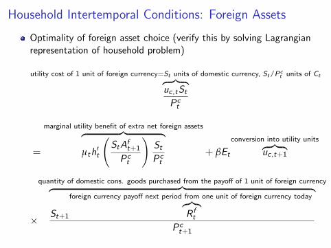
Household Intertemporal Conditions: Foreign Assets

Optimality of foreign asset choice (verify this by solving Lagrangianrepresentation of household problem)

utility cost of 1 unit of foreign currency=S

t

units of domestic currency, S

t

/P

c

t

units of C

tz }| {u

c,t

S

t

P

c

t

=

marginal utility benefit of extra net foreign assetsz }| {

µt

h

0t

S

t

A

f

t+1

P

c

t

!S

t

P

c

t

+ bEt

conversion into utility unitsz }| {u

c,t+1

⇥

quantity of domestic cons. goods purchased from the payo↵ of 1 unit of foreign currencyz }| {

S

t+1

foreign currency payo↵ next period from one unit of foreign currency todayz}|{R

f

t

P

c

t+1

Household Intertemporal Conditions: Foreign Assets

First order condition:

S

t

P

c

t

C

t

= h

0t

A

t

S

t

A

f

t+1

A

t

P

t

p

c

t

!S

t

P

c

t

+ bEt

S

t+1

R

f

t

P

c

t+1

C

t+1

Scaling:

1

c

t

= h

0t

✓A

t

a

f

t

p

c

t

◆+ bE

t

s

t+1

R

f

t

pc

t+1

c

t+1

exp (Da

t+1

),

c

t

⌘ C

t

A

t

, aft

⌘S

t

A

f

t+1

P

t

A

t

, st

⌘ S

t

S

t�1

= y˜

S

t

˜

S

t�1

(14)

Utility Value of Net Foreign AssetsSuppose that (for reasons not modeled) people have a target level ofnet foreign assets, summarized in the function, h

t

:

h

t

S

t

A

f

t+1

P

c

t

!= �1

2g

0

@A

t

S

t

A

f

t+1

A

t

P

t

p

c

t

� A

t

Ut

A

t

1

A2

= �1

2g

✓a

f

t

p

c

t

� Ut

◆2

.

From previous slide:

1

c

t

= h

0t

A

t

a

f

t+1

p

c

t

!+ bE

t

s

t+1

R

f

t

pc

t+1

c

t+1

exp (Da

t+1

)

Then,

1

c

t

= �g

✓a

f

t

p

c

t

� Ut

◆+ bE

t

s

t+1

R

f

t

pc

t+1

c

t+1

exp (Da

t+1

)(7)

Why Put Net Foreign Assets in the Utility Function?

The primary motivation is technical and is described in, for example,Schmitt-Grohe and Uribe.

Because the domestic economy is assumed to be small, it has noimpact on R

f

t

, the return on foreign assets.I From the point of view of domestic residents, the foreign asset

represents a constant returns investment technology.I The consequence is that there does not exist a steady state level of net

foreign assets that is independent of the initial net foreign assetposition.

I Why? The answer resembles why there is no steady state capital stockindependent of initial capital in the so-called Ak model:

FThat is, if k starts low, there is no incentive to raise investment sharply

to raise k to some steady state level. That’s because the marginal

product of capital, A, is not higher when k is low.

FSimilarly, when k is high, there is no reason to let the stock of capital

fall. That is, when k is high, A is not lower.

Why Put Net Foreign Assets in the Utility Function?Standard solution methods assume that variables have a steady statethat is independent of initial conditions.Small open economy models require a small adjustment.Consider the first order condition for foreign assets:

1

c

t

=

second partz }| {

�g

✓a

f

t

p

c

t

� Ut

◆+

first partz }| {

bEt

s

t+1

R

f

t

pc

t+1

c

t+1

exp (Da

t+1

)(7)

The payo↵ on the foreign asset corresponds to the two parts of theterm on the right of the equality:

I First part: normal part of the return on the foreign assets, stemmingfrom their cash payo↵.

I Second part: makes overall return higher when households’ net foreignasset position is below target, U

t

, giving households incentive to

accumulate more assets. Similarly, the overall return is lower whenthe net foreign asset position is above target, giving households anincentive to accumulate less.

So, model has a unique steady state, for g > 0.

Final Domestic Consumption Goods

Produced by representative, competitive firm using:

C

t

=

"

(1� wc

)1

hc

⇣C

d

t

⌘ hc

�1

hc + w

1

hc

c

(Cm

t

)hc

�1

hc

# hc

hc

�1

where

C

d

t

domestic homogeneous output good, price P

t

C

m

t

imported good, price P

m

t

�⌘ S

t

P

f

t

�

C

t

final consumption good, Pc

t

hc

elasticity of substitution, domestic and foreign goods.

The firm takes the prices, Pt

,Pm

t

,Pc

t

, as given and beyond its control.

Final Domestic Consumption Goods

Profit maximization by representative firm:

maxC

t

,C

m

t

,C

d

t

P

c

t

C

t

� P

m

t

C

m

t

� P

t

C

d

t

,

subject to production function.

First order conditions associated with maximization:

C

m

t

: P

c

t

=⇣

wc

C

t

C

m

t

⌘ 1

hc

z }| {dC

t

dC

m

t

= P

m

t

, C

d

t

: P

c

t

=

✓(1�w

c

) C

t

C

d

t

◆ 1

hc

z}|{dC

t

dC

d

t

= P

t

so that the demand functions are:

C

m

t

= wc

✓P

c

t

P

m

t

◆hc

C

t

, C

d

t

= (1� wc

)

✓P

c

t

P

t

◆hc

C

t

.

Final Good Prices

Substituting demand functions back into the production function:

C

t

= [(1� wc

)1

hc

✓C

t

✓P

c

t

P

t

◆hc

(1� wc

)

◆ hc

�1

hc

+ w1

hc

c

✓w

c

✓P

c

t

P

m

t

◆hc

C

t

◆ hc

�1

hc

]hc

hc

�1 ,

to obtain,

p

c

t

=

marginal cost, in units of the homogeneous goodz }| {h(1� w

c

) + wc

(pmt

)1�hc

i 1

1�hc (8)

p

c

t

⌘ P

c

t

P

t

, p

m

t

⌘ P

m

t

P

t

.

Pass-Through

Multiplying (8) by P

t

’price = marginal cost’:

P

c

t

=h(1� w

c

) (Pt

)1�hc + w

c

(Pm

t

)1�hc

i 1

1�hc ,

or, using P

m

t

= S

t

P

f

t

:

P

c

t

=

(1� w

c

) (Pt

)1�hc + w

c

⇣S

t

P

f

t

⌘1�h

c

� 1

1�hc

.

Note that if the exchange rate depreciates, i.e., St

rises, thenmarginal cost rises so that the depreciation is ’passed through’marginal cost and into the final good price, Pc

t

. This pass-throughoccurs, no matter how sticky the prices underlying P

t

are.

The high degree of pass through in this model reflects its simplicity.See CTW for a discussion of how this model can be modified to slowdown the pass through of exchange rate changes into final goodprices.

Consumer Price Inflation

Consumption good inflation and homogeneous good inflation:

pc

t

⌘ P

c

t

P

c

t�1

=P

t

p

c

t

P

t�1

p

c

t�1

= pt

"(1� w

c

) + wc

(pmt

)1�hc

(1� wc

) + wc

�p

m

t�1

�1�h

c

# 1

1�hc

(10)

Real Exchange RateReal Exchange Rate, q

p

m

t

=P

c

t

P

c

t

zero profits for importers, P

m

t

= S

t

P

f

tz}|{P

m

t

P

t

= p

c

t

⇥real exchange rate, q

t

⌘ S

t

P

f

t

P

c

tz}|{q

t

(9)

Scaling:

1zero profit condition for exportersz}|{

=S

t

P

x

t

P

t

=P

c

t

S

t

P

f

t

P

x

t

P

t

P

c

t

P

f

t

= q

t

p

x

t

p

c

t

(12)

Also,

q

t

q

t�1

= s

t

pf

t

pc

t

, (13), pf

t

⌘ P

f

t

P

f

t�1

Exports

Foreign demand for domestic goods:

X

t

=

✓P

x

t

P

f

t

◆�hf

Y

f

t

= (pxt

)�hf

Y

f

t

,

terms of tradez}|{p

x

t

=P

x

t

P

f

t

Y

f

t

foreign outputP

f

t

foreign currency price of foreign goodP

x

t

foreign currency price of export good

Foreign demand is exogenous to the domestic economy.

Balanced GrowthThe model exhibits growth when A

t

grows over time.We require the growth to be balanced, so that when growing variablesare scaled by A

t

the ratios converge in steady state.Mathematically, balanced growth requires that after all variables arescaled by A

t

, At

itself disappears from the system.I This places certain restrictions on preferences and technology,

restrictions which our model satisfies.

So, in the case of Y f

t

, balanced growth requires that Y f

t

grows at thesame rate as A

t

.An obvious way to proceed is to assume

Y

f

t

= y

f

t

A

t

,

where y

f

t

is an exogenous shock to Y

f

t

. But, this formulation impliesthat a shock to technology simultaneously expands the demand forexports.

I Seems implausible.I Inconvenient when we compute impulse response functions. Here, we

want to study the e↵ects of a disturbance that originates in just onepart of the system.

Exports

Preceding slide suggests we want to express Y f

t

in the following form:

Y

f

t

= y

f

t

Z

t

,

where Z

t

grows with A

t

, yet Zt

responds extremely slowly to A

t

.

We apply the approach in Christiano-Trabandt-Walentin (2011,section 2.3):

Y

f

t

= y

f

t

Z

t

,Zt

= A

1�dt

Z

dt�1

, 0 < d < 1,

z

t

⌘ Z

t

A

t

=

✓A

t�1

A

t

Z

t�1

A

t�1

◆d

= exp (�dDa

t

) zdt�1

(18)

x

t

= (pxt

)�hf

y

f

t

z

t

(11)

Note: with d close, but less than, unity:I

Z

t

grows at the same as At

in the sense that Zt

/A

t

converges to aconstant in steady state.

IZ

t

hardly responds to a shock to a shock in A

t

.

Homogeneous Goods Market Clearing

Clearing in domestic homogeneous goods market:

output of domestic homogeneous good, Y

t

= uses of domestic homogeneous goods

or,

Y

t

=

goods used in production of final consumption, C

tz}|{C

d

t

+

exportsz}|{X

t

+

govenmentz}|{G

t

= (1� wc

)(pct

)hc

C

t

+ X

t

+ G

t

.

Aggregate Employment and Uses of Homogeneous Goods

Substituting out in previous expression for Yt

:

A

t

p

⇤t

N

t

= (1� wc

) (pct

)hc

C

t

+ X

t

+ G

t

,

or,p

⇤t

N

t

= (1� wc

) (pct

)hc

c

t

+ x

t

+ g

t

z

t

, (6)

c

t

⌘ C

t

A

t

, x

t

⌘ X

t

A

t

, G

t

= g

t

Z

t

, zt

=Z

t

A

t

.

Also,

y

t

=Y

t

A

t

= p

⇤t

N

t

(16)

For an extended discussion of (16), see this.

Balance of Payments

expenses on imports net of receipts from exports equals flow offinancial assets abroad.

acquisition of new net foreign assets, in domestic currency unitsz }| {S

t

A

f

t+1

+ expenses on importst

=receipts from exportst

+

receipts from existing stock of net foreign assetsz }| {S

t

R

f

t�1

A

f

t

Balance of Payments, the Pieces

Exports and imports:

expenses on importst

= S

t

P

f

t

wc

✓p

c

t

p

m

t

◆hc

C

t

receipts from exportst

= S

t

P

x

t

X

t

.

Balance of payments:

S

t

A

f

t+1

+ S

t

P

f

t

wc

✓p

c

t

p

m

t

◆hc

C

t

= S

t

P

x

t

X

t

+ S

t

R

f

t�1

A

f

t

.

Balance of Payments, Scaling

Scaling by P

t

A

t

:

S

t

A

f

t+1

P

t

A

t

+S

t

P

f

t

P

t

wc

✓p

c

t

p

m

t

◆hc

c

t

=S

t

P

x

t

P

t

x

t

+S

t

R

f

t�1

A

f

t

P

t

A

t

,

or,

a

f

t

+ p

m

t

wc

✓p

c

t

p

m

t

◆hc

c

t

= p

c

t

q

t

p

x

t

x

t

+s

t

R

f

t�1

a

f

t�1

pt

exp (Da

t

), (15)

where a

f

t

is ’scaled, homogeneous goods value of net foreign assets’

Gross Domestic ProductGDP: ’C + I + G + Net Exports’.

I Problem: these are di↵erent goods, with di↵erent prices.

GDP in domestic consumption units - nominal divided by P

c

t

:

GDP

t

⌘

nominal expenditures on consumptionz }| {P

c

t

A

t

c

t

+

nominal government expz }| {P

t

g

t

Z

t

P

c

t

+�

nominal importsz }| {

S

t

P

f

t

wc

✓p

c

t

p

m

t

◆hc

C

t

+

nominal exportsz }| {x

t

P

t

A

t

P

c

t

=A

t

⌘gdp

t

, scaled by A

tz }| {"c

t

+g

t

z

t

p

c

t

�✓p

m

t

p

c

t

◆1�hc

wc

c

t

+x

t

p

c

t

#

So, GDP (in consumption units) growth is:

log (GDPt

)� log (GDt�1

) = Da

t

+ log (gdpt

)� log (gdpt�1

) .

Pulling the Equations TogetherThe 18 endogenous variables:

K

t

,Ft

,Nt

, yt

,pt

, ct

, p⇤t

,Rt

, aft

, pmt

, pct

, qt

, pxt

,pc

t

, xt

, st

, eSt

, zt

The 8 exogenous variables: Ut

, tt

,Da

t

, #R,t

, gt

,pf

t

, y ft

,R f

t

Equilibrium conditions resembling those in closed economy:

K

t

=# (1� n)

# � 1exp (t

t

)Njt

y

t

p

c

t

+ bqEt

(1

pt+1

)�#K

t+1

(1)

F

t

=y

t

c

t

+ E

t

p#�1

t+1

bqFt+1

(2)K

t

F

t

=

1� qp#�1

t

1-q

� 1

1�#

(3)

p

⇤t

=

0

@(1� q)

1� q (p

t

)#�1

1� q

! ##�1

+qp#

t

p

⇤t�1

1

A�1

(4)

1

c

t

= bEt

R

t

pc

t+1

c

t+1

exp (Da

t+1

)(5)

y

t

= (1� wc

) (pct

)hc

c

t

+ x

t

+ g

t

z

t

(6)

Pulling the Equations Together

1

c

t

= �g

✓a

f

t

p

c

t

� Ut

◆+ bE

t

s

t+1

R

f

t

pc

t+1

c

t+1

exp (Da

t+1

)(7)

p

c

t

=h(1� w

c

) + wc

(pmt

)1�hc

i 1

1�hc (8)

p

m

t

= p

c

t

q

t

(9)

pc

t

= pt

"(1� w

c

) + wc

(pmt

)1�hc

(1� wc

) + wc

�p

m

t�1

�1�h

c

# 1

1�hc

(10)

x

t

= (pxt

)�hf

y

f

t

z

t

(11)

1 = q

t

p

x

t

p

c

t

(12)

Pulling the Equations TogetherLast equations:

q

t

q

t�1

= s

t

pf

t

pc

t

(13)

s

t

= yeS

t

eS

t�1

(14)

a

f

t

+ p

m

t

wc

✓p

c

t

p

m

t

◆hc

c

t

= p

c

t

q

t

p

x

t

x

t

+s

t

R

f

t�1

a

f

t�1

pt

exp (Da

t

)(15)

y

t

= p

⇤t

N

t

(16)

log

✓R

t

R

◆= r

R

log

✓R

t�1

R

◆

+ (1� rR

)Et

[rp log

✓pc

t

¯pc

◆+ r

y

log

✓y

t

y

◆+ r

S

log

⇣eS

t

⌘]

+ #R,t

(17)

z

t

= exp (�dDa

t

) zdt�1

(18)

Summing Up

We now have 18 equations in 18 unknowns.

Parameters:

d, q,wc

, b, hc

, hg

, hf

, #, n,y, j,g, t,R f , y f ,pf ,Da, rR

, rp, ry , rS

, ¯pc ,U

Next:I compute steady stateI dynamic model analysis.

FPredictability of exchange rate (url: Eichenbaum-Johanssen-Rebelo)

FUncovered Interest Rate Parity

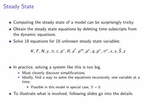
Steady State

Computing the steady state of a model can be surprisingly tricky.

Obtain the steady state equations by deleting time subscripts fromthe dynamic equations.

Solve 18 equations for 18 unknown steady state variables:

K ,F ,N, y ,p, c , p⇤,R , af , pm, pc , q, px ,pc , x , s, eS , z

In practice, solving a system like this is too big.I Must cleverly discover simplifications.I Ideally, find a way to solve the equations recursively, one variable at a

time.F

Possible in this model in special case, U = 0.

To illustrate what is involved, following slides go into the details.

Steady State: Some Easy VariablesForeign variables fixed exogenously: pf , R f .

I pf and R

f assumed to be linked by foreigners’ intertemporal Eulerequation, same as domestic:

1 = bR

f

pf exp (Da), pf

t

⌘ P

f

t

P

f

t�1

(exogenous)

Domestic monetary policy forces pc = ¯pc , ¯pc ˜ steady state ofinflation target.Additional steady state equations:

p ⌘ P

t

P

t�1

= ¯pc (inflation target) (10)

pf = pc

/y (13), s = y (14)

R = sR

f , (’UIP holds in steady state’) (5) and (7)

Easily verified that domestic intertemporal Euler equation is satisfied:

1 = bR

pc exp (Da)(5)

Steady State: Some Easy VariablesTack Yun distortion:

p

⇤ =1�qp#

1�q⇣1�qp#�1

1�q

⌘ ##�1

(4)

The growth factor:

z = exp

✓� d

1� dDa

◆(18)

Euler equation for foreign assets, (7), in steady state:

1 = �gc

✓a

f

p

c

� U◆+ b

sR

f

pc exp (Da)(7).

Combine with domestic Euler equation, (5), and sR

f = R , conclude:

a

f

p

c

= U.

Not ready for computations, since has two unknowns.

Steady StateLet h

g

denote the share of government consumption in

homogeneous output:

g = hg

y/z .

Using the latter and (16), (6) reduces to:

0 = (1� wc

) (pc)hc

c + x � (1� hg

)Np⇤ (6)

Making use of (12), (15) becomes:

0 = p

mwc

✓p

c

p

m

◆hc

c � x �✓1

b� 1

◆a

f (15)

Substituting out for x from (15) into (6), using (8) and rearranging:

p

c

c =

✓1

b� 1

◆a

f + (1� hg

)Np⇤ (6),

which says that the value of scaled consumption in steady stateequals interest on foreign assets plus homogeneous output, minusgovernment consumption.

Steady State

Using (2) and (3) to substitute out for K and F in (1):

0 =# (1� n)

# � 1N

1+jp

⇤p

c +(bqp# � 1) p⇤Nc (1� p#�1bq)

1� qp#�1

1� q

� 1

1�#

(1)

After rearranging:

N

jp

c

c =# � 1

# (1� n)(1� bqp#)(1� p#�1bq)

1� qp#�1

1� q

� 1

1�#

(1)

Substituting out for pcc from (6):

0 =N

1+j + b

1

N

j � b

2

, (1)

b

1

=

⇣1

b � 1⌘a

f

(1� hg

) p⇤,

b

2

=# � 1

(1� hg

) p⇤# (1� n)(1� bqp#)(1� p#�1bq)

1� qp#�1

1� q

� 1

1�#

.

Steady State: Special Case, U = 0

In this case, af = 0. Then, b1

= 0 in previous slide and

N = b

1

1+j

2

.

Compute p

c

c using (6).

But, not obvious how to compute the other variables, e.g., pc , px , ...one at a time, in a nice recursive sequence.

I We now switch to a nonlinear search.I We do so in a way that maximizes the chance we discover multiple

steady state if this is the case (it appears not to be in this model).

Steady State: Non-recursive, Iterative Approach

To illustrate how we proceed, consider the following joint system oftwo equations in two unknowns, y , x :

f (x , y) = 0

g (x , y) = 0

I We solve this system as a nested set of two one-dimensional problems.

For each fixed x let y (x) denote the value of y that solves theone-dimensional problem, g (x , y) = 0.

I The problem of finding y (x) is the inner loop problem, and y is theinner loop variable.

I For the outer loop problem, find a value for the outer loop variable, x ,such that f (x , y (x)) = 0.

Steady State: Non-recursive, Iterative ApproachIt is convenient to define the following variable: ˜j = p

c

q.I

˜j is the outer loop variable in our solution strategy.

We now define the inner loop problem. Solve:

p

m = ˜j (9) and p

x =1

˜j(12)

p

c =h(1� w

c

) + wc

(pm)1�hc

i 1

1�hc (8)

q =˜j

p

c

a

f = p

cU.

Then, solve (1) for N and (6) for pcc .I When a

f 6= 0 this an inner loop nonlinear search is required to find N.I Actually, when j = 1 the nonlinear search simplifies to finding the

zeros of a second order polynomial.

With p

c

c in hand, c is recovered by dividing with respect to p

c from(8).Use (15) to compute x . Also, (2) and (3) can be used to compute K

and F .I Adjust the value of the outer loop variable, ˜j, until the outer loop

problem is solved, that is, (11) is satisfied.

Model Solution and Parameter ValuesWe use standard linearization techniques to solve the model.This requires having values for the model parameters. We adopt thefollowing:

¯pc = 1.005 U = 0 b = 1.03�1/4

q = 3/4 j = 1 # = 61� n = #�1

# hc

= 5 wc

= 0.4hg

= 0.3 g = 2 hf

= 1.5rR

= 0.9 rp = 1.5 r

y

= 0.15rS

=0.02 y=1.0118 Da=0˜j=1 t=0 d=0.999

We activated three shocks in the system, Da

t

, a shock to U, and themonetary policy shock, #

R,t

. The monetary policy shock is iid withstandard deviation, 0.0025. The other two shocks are scalar AR(1)’s.The autocorrelation of the technology and U shocks are 0.90 and0.95, respectively. Their standard deviations are 0.01 and 0.05.In the following, we discuss the values assigned to the non-standardparameters, r

S

and g.

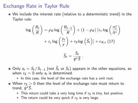
Exchange Rate in Taylor Rule

We include the interest rate (relative to a deterministic trend) in theTaylor rule:

log

✓R

t

R

◆= r

R

log

✓R

t�1

R

◆+ (1� r

R

) [rp log

✓pc

t

¯pc

◆

+ r

y

log

✓y

t

y

◆+ r

S

log

⇣eS

t

⌘] + #

R,t

(17)

eS

t

=S

t

yt

¯

S

.

Only s

t

= S

t

/S

t�1

(not eSt

or St

) appears in the other equations, sowhen r

S

= 0 only s

t

is determined.I In this case, the level of the exchange rate has a unit root.

When r

S

> 0 then the level of the exchange rate must return totrend, yt

¯

S .

I This return could take a very long time if rS

is tiny, but positive.I The return could be very quick if r

S

is very large.

Exchange Rate in Taylor Rule

Should we put the exchange rate in Taylor rule?I Is there evidence that policymakers keep the exchange rate to some

form of target?

Some casual evidence described below suggests that in many cases St

can be interpreted as exhibiting a return to trend, though thishappens at best over the longer run.

I See the following slides....

Long-run return to trend in exchange rate may be part of theexplanation for the ’uncovered interest parity’ puzzle. See below.

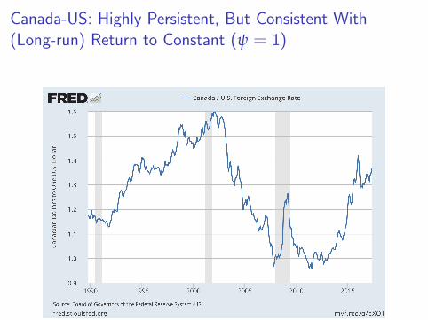
Canada-US: Highly Persistent, But Consistent With(Long-run) Return to Constant (y = 1)

China-US: Persistent, but Change in Regime (i.e., changein the value of y) in mid 1990s?

Euro-US: Highly Persistent, but Around DollarDepreciation Trend (y > 1)?

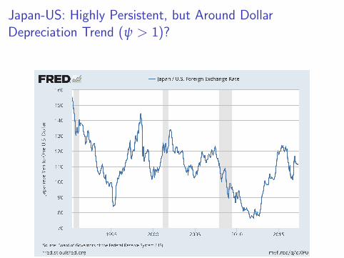
Japan-US: Highly Persistent, but Around DollarDepreciation Trend (y > 1)?

Mexico-US: Highly Persistent, but Around DollarAppreciation Trend (y < 1)?

US and its Major Trading Partners (Trade-weighted):Highly Persistent, Around (Slight) Dollar DepreciationTrend (y > 1)?

Empirical Measurement of ’Long-Run Return to Trend’

Convenient to consider the following reduced form, AR(1)representation of log exchange rate (suppose y = 1):

log (St

) = (1� r) log ( ¯

S) + r log (St�1

) + #t

,

so that

log(St+j

) =�1� rj

�log ( ¯

S) + rj log(St

)

+ #t+j

+ r#t+j�1

+ ...+ rj�1#t

or,

E

t

log (St+j

)� log (St

) = b (j) (log(St

)� log ( ¯

S)) , b (j) ⌘�rj � 1

�

Get full return to trend if b (j) ! �1 as j ! •.

Empirical Measurement of ’Long-Run Return to Trend’

Expected change in exchange rate and gap:

E

t

log (St+j

)� log (St

) = b (j) (log(St

)� log ( ¯

S)) , b (j) ⌘�rj � 1

�

The function, b (j) determines the trend behavior of St

.I If r = 1 then b (j) = 0 for all j and exchange rate never moves back to

any trend.F

model may capture this case with rS

= 0, when only St

/St�1

(i.e., not

St

itself) appears in the system.

I If r < 1, but r is close to unity, then b (j) ' 0 for j small butb (j) ! �1 as j ! •.

FIn this case, get return to trend behavior over the long-term, but little

evidence of that in the short term (resembles behavior of actual interest

rates).

FIn the model, this is the case, r

S

> 0 but close to zero.

Can estimate b (j) by ordinary least squares regression.

b (j) for Monthly Exchange Rate of US and its MajorTrading Partners (Trade-weighted)These calculations confirm visual impression that b (j) ' 0 for low valuesof j (so, weak return to trend in short run) and b (j) ' �1 for large j .

10 20 30 40 50 60 70 80 90 100 110 120j lags

-1

-0.9

-0.8

-0.7

-0.6

-0.5

-0.4

-0.3

-0.2

-0.1

-(j

)

E[log(St+j)]! log(St) = ,(j) +-(j)log(St), Monthly Data

Model Prediction for b (j) as a Function of jFor each j , estimated a (j) , b (j) by least squares using 100,000 simulatedquarterly data with only monetary policy shocks from three di↵erentversions of the model, according to value of r

S

. Get pattern of empiricaldata (ignoring mismatch of sampling frequency!) by selecting r

S

' 0.02.

10 20 30 40 50 60 70 80 90 100j lags

-1

-0.9

-0.8

-0.7

-0.6

-0.5

-0.4

-0.3

-0.2

-0.1

-(j

)

E[log(St+j)]! log(St) = ,(j) +-(j)log(St), Model is quarterly

baseline rS = 0:02

small rS = 0:0002

large rS = 20

Interest Parity

The model implies a relationship between interest rates and theexchange rate.

I That relationship has been the subject of much research.

That relationship is best understood by linearizing a portion of themodel.

Interest Parity

Combine the household’s intertemporal first order conditions fordomestic and foreign bonds, (6) and (7):

g

✓a

f

t

p

c

t

� Ut

◆= E

t

b

s

t+1

R

f

t

� R

t

pc

t+1

c

t+1

exp (Da

t+1

)

�

Linearizing the object in square brackets (using sR

f = R):

dbs

t+1

R

f

t

� R

t

pc

t+1

c

t+1

exp (Da

t+1

)=

1

c

⇣s

t+1

+ ˆ

R

f

t

� ˆ

R

t

⌘

where

x

t

⌘ x

t

� x

x

=dx

t

x

.

Also,

d

✓a

f

t

p

c

t

� Ut

◆=

1

p

c

da

f

t

� U ˆ

p

c

t

� dUt

Interest Parity

From the previous slide:

ˆ

R

t

=

Expected return, in domestic currency, to household that invests in R

f

tz }| {ˆ

R

f

t

+ E

t

[st+1

] + ˆFt

ˆFt

⌘ cg

✓� 1

p

c

da

f

t

+ Up

c

t

+ dUt

◆

Uncovered Interest Parity (UIP):

ˆ

R

t

= ˆ

R

f

t

+ E

t

[st+1

]

I Under UIP, households only consider the expected returns on di↵erentassets, so equilibrium requires that the expected returns are equated.

I Although UIP seems to hold ’in the long run’, it does not appear tohold consistently in the short run.

I Researchers have often used

ˆFt

as a way to account for short-run

failure of UIP.

FWe have introduced it to ensure a steady state for net foreign assets.

Modified Uncovered Interest ParityMUIP:

ˆ

R

t

� ˆ

R

f

t

= E

t

[st+1

] + ˆFt

I ˆFt

often referred to as ’domestic risk premium term’.

I When

ˆFt

> 0, traders require higher (exchange rate adjusted)

domestic rate of interest to be indifferent between domestic and

foreign assets.

Note

1+ x

t

= 1+dx

t

x

= 1+x

t

� x

x

=x

t

x

so,bxt

' log (1+ bxt

) = logx

t

x

Then:

log(St+1

)� log(St

) = r

t

� r

f

t

� ˆFt

+ u

t

,

where

r

t

= log

R

t

R

, r ft

= log

R

f

t

R

f

, u

t

? variables dated t and earlier

Modified Uncovered Interest ParityMIUP:

log St+1

= r

t

� r

f

t

+ log St

� ˆFt

+ u

t

log St+2

= r

t+1

� r

f

t+1

+ log St+1

� ˆFt+1

+ u

t+1

= r

t+1

� r

f

t+1

+ r

t

� r

f

t

+ log St

� ˆFt

� ˆFt+1

+ u

t

+ u

t+1

Then,

log St+j

= r

t

� r

f

t

+ r

t+1

� r

f

t+1

+ ..+ r

t+j�1

� r

f

t+j�1

+ log St

� ˆFt

� ...� ˆFt+j�1

+ u

t

+ ...+ u

t+j�1

A lot of volatility in S

t

under UIP and MUIP (i.e., ˆFt

= 0)I Suppose r

t

� r

f

t

jumps at t and returns to its initial condition fromabove, then exchange rate depreciates,log S

t+j

� log St

� 0, for all

j > 0.

I With r

S

> 0, E

t

log St+j

converges, as j ! •, to its unshocked path.So, log S

t

drops in period t.

Impulse Responses

Much of the economics of a model can be found by studying itsimpulse responses.

Next, we consider shocks to technology, monetary policy and ’capitalflight’: Da

t

, #R,t

,Ut

Responses to Technology Shock

10 20 30 40

4

6

8

100*logdev,ss

log Y

10 20 30 40

6

8

10

100*logdev,ss

log C

10 20 30 40

0.5

1

1.5

2

2.5

dev,ss

R (APR)

10 20 30 40

4

6

8

10

100*logdev,ss

log S

10 20 30 40

-10123

100*logdev,ss

log N

10 20 30 40

2

4

6

8dev

from

ss

:c (APR)

10 20 30 40

0.81

1.21.41.6

100*logdev,ss

log q

10 20 30 40-2

-1

0

1

level

#10-3 S $Af=Pc

10 20 30 40

-2.5

-2

-1.5

100*logdev,ss

ToT

10 20 30 40

2

3

4

100*logdev,ss

Exports

10 20 30 402

3

4

100*logdev,ss

Imports

10 20 30 40

2

4

6

8

100*logdev,ss

Technology

10 20 30 40

2

4

6

8

100*logdev,ss

Y/N

10 20 30 40

0.1

0.2

0.3

100*logdev,ss

Export demand, Y f

10 20 30 40

0.3420.3440.3460.3480.35

level

exports

imports

response to technology shock, . =2, rS =0.02, ;R =0.9

10 20 30 40

0.1

0.2

0.3

100*logdev,ss

gov't consumption

Interpreting Responses to Tech ShockThe 3,4 chart displays the impulse. The state of technology, A

t

,jumps 1% in the period of the shock and asymptotically it jumps 10%.The strong wealth e↵ect associated with the shock drives upconsumption and imports (the latter are an input into the productionof consumption goods). See the 1,2 and 3,3 charts.Rise in imports drives depreciation (1,4 chart).The rise in employment and the exchange rate contribute to theincreased production costs that underly the (sharp) rise in inflation inthe 2,2 chart. We can see the big role played by exchange ratepass-through here.The rise in inflation contributes, via the monetary policy rule, to a risein the domestic rate of interest. After a brief initial rise in net foreignassets, those assets drop.The increase in productivity contributes to a drop in the terms oftrade, px

t

, which stimulates exports. Exports and imports both rise byroughly similar amounts (see 4,3).The shift in foreign demand, Y f

t

, for exports and in governmentspending are small because d is so close to unity (see 4,2 and 4,4).

Responses to U Shock (’Capital Outflow Shock’)

10 20 30 400

1

2

100*logdev,ss

log(Yt)

10 20 30 40

-1

-0.5

0

100*logdev,ss

log(Ct)

10 20 30 400

0.2

0.4

0.6

0.8

dev,ss

Domestic Risk Free Rate (APR)

10 20 30 400

1

2

100*dev,ss

log( ~St)

10 20 30 400

1

2

logdev,ss

log(Nt)

10 20 30 40

-2

0

2

4

dev,ss

Consumer Price In.ation (APR)

10 20 30 400

0.5

1

1.5

logdev,ss

log(qt)

10 20 30 40

0.01

0.02

0.03

0.04

level

Real Foreign Assets

10 20 30 40

-2

-1

0

logdev,ss

log(Pxt =Pf

t )

10 20 30 400

1

2

3

logdev,ss

log(Xt)

response to upsilon shock

10 20 30 40

-6

-4

-2

0logdev,ss

log(Imports)

Interpreting Responses to U Shock

The capital outflow shock drives households to acquire foreign assets(chart 2,4) and this leads to an immediate nominal depreciation(chart 1,4).

The depreciation stimulates exports by reducing the terms of trade,p

x

t

. To see how, note

p

x

t

⌘ P

x

t

P

f

t

=S

t

P

x

t

S

t

P

f

t

=P

t

S

t

P

f

t

.

Sticky prices make P

t

slow to move and P

f

t

is exogenous. So, weexpect a jump in S

t

to produce a fall in the terms of trade andstimulate exports. See chart 3,1.

The rise in output and costs (together with the strong pass-throughfrom the exchange rate) lead to a sharp jump in inflation, so thatmonetary policy generates a rise in the interest rate (charts 1,3 and2,2).

Interpreting Responses to U Shock, cnt’d

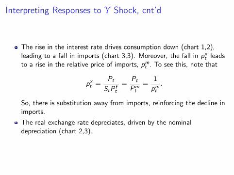
The rise in the interest rate drives consumption down (chart 1,2),leading to a fall in imports (chart 3,3). Moreover, the fall in p

x

t

leadsto a rise in the relative price of imports, pm

t

. To see this, note that

p

x

t

=P

t

S

t

P

f

t

=P

t

P

m

t

=1

p

m

t

.

So, there is substitution away from imports, reinforcing the decline inimports.

The real exchange rate depreciates, driven by the nominaldepreciation (chart 2,3).

Responses to Money Policy Shock

10 20 30 40-0.2

-0.15

-0.1

-0.05

100*logdev,ss

log(Yt)

10 20 30 40

-0.2

-0.15

-0.1

-0.05

100*logdev,ss

log(Ct)

10 20 30 40

0.05

0.1

0.15

dev,ss

Domestic Risk Free Rate (APR)

10 20 30 40

-0.2

-0.15

-0.1

100*dev,ss

log( ~St)

10 20 30 40

-0.2

-0.1

0

logdev,ss

log(Nt)

10 20 30 40

-0.4

-0.2

0

dev,ss

Consumer Price In.ation (APR)

10 20 30 40-0.05-0.04-0.03-0.02-0.01

logdev,ss

log(qt)

10 20 30 40

-2

-1

0

level

#10-4Real Foreign Assets

10 20 30 40

0.02

0.04

0.06

0.08

logdev,ss

log(Pxt =Pf

t )

10 20 30 40

-0.12-0.1

-0.08-0.06-0.04-0.02

logdev,ss

log(Xt)

response to R shock

10 20 30 40

-0.06

-0.04

-0.02

logdev,ss

log(Imports)

Interpreting Responses to Money Policy Shock

The monetary policy shock drives up R

t

(see chart 1,3), causingconsumption to drop (see 1,2).

This leads to a fall in production and employment, and, by reducingcosts, to a drop in inflation (charts 1,1, 2,1 and 2,2).

The high interest rate causes exchange rate to be depreciated. Thee↵ects of pass-through would, other things the same, drive inflationup. In fact, the inflation rate drops. But, the amount of the drop ismuch smaller than we’ve seen in the other experiments. Sopass-through and the other cost factors roughly cancel.

The depreciated exchange rate leads to a rise in the terms of trade(see the discussion of previous shocks), and, hence a drop in exports(see charts 3,1 and 3,2).

The fall in consumption leads to a fall in imports (see chart 3,3).

Interpreting Responses to Money Policy Shock, cnt’d

The rise in the interest rate leads to a fall in foreign assets. Becausethe shock hits the economy when it is in steady state, the holdings offoreign assets are now below target. This adds a positive,non-pecuniary, return to those assets because g > 0. Thus, tradersrequire a higher return on domestic assets to be willing to hold both.This explains why they are willing to hold both, even though after theshock they receive a higher domestic interest rate and the e↵ectiveforeign interest rate is lower because the foreign currency is expectedto depreciate (i.e., the domestic currency is expected to appreciate).See the downward-sloped portion of the exchange rate trajectory inchart 1,4).

Because the exchange rate is in the monetary policy rule, it musteventually return to trend. This guarantees that eventually theexchange rate must be higher than it was in the period of thecontractionary monetary action, when it exhibits a discreteappreciation. See the upward-sloped portion of the exchange ratetrajectory in chart 1,4.

Modified Uncovered Interest ParityMIUP:

log St+j

= r

t

� r

f

t

+ r

t+1

� r

f

t+1

+ ..+ r

t+j�1

� r

f

t+j�1

+ log St

� ˆFt

� ...� ˆFt+j�1

+ u

t

+ ...+ u

t+j�1

Long term interest rate in model:

r

(j)t

= E

t

[rt

+ ...+ r

t+j�1

] = r

t

+ ...+ r

t+j�1

+ ht,t+j

,

ht,t+j

? information dated t and ealier

Rewriting MUIP:

log St+j

= r

(j)t

� r

f (j)t

+ log St

� ˆFt

� ...� ˆFt+j�1

+ wt+j

wt+j

= u

t

+ ...+ u

t+j�1

+ ht,t+j

? info dated t and ealier

UIP (i.e., ˆFt

= 0)I Under UIP, regression of logS

t+j

� logS

t

on date t, j-period interestrate di↵erential should have unit coe�cient, for all j > 0.

I UIP puzzle: Chinn and Meredith (2012) - when j small, UIP predictionviolated; when j large, UIP prediction satisfied.

Impact of g, rS

, rR

on MUIP

10 20 30 40

-2

-1

0

logdev,ss

#10-3 log(Yt)

10 20 30 40

-2

-1

0

logdev,ss

#10-3 log(Ct)

10 20 30 40

5

5.05

5.1

5.15

dev,ss

Rt (APR)

10 20 30 40

-2-1.5-1

-0.5

#10-3 log( ~St)

10 20 30 40

-2

-1

0#10-3 log(Nt)

10 20 30 40-0.6

-0.4

-0.2

0Consumer Price In.ation (APR)

10 20 30 40

-8-6-4-20#10-4 log(qt)

10 20 30 40-15

-10

-5

0 #10-4Real Foreign Assets

10 20 30 400

5

10

15#10-4 log(Px

t =Pft )

10 20 30 40

-2

-1

0#10-3 log(Xt)

Benchmark

low .

High rS

low ;R

response to monetary shock

10 20 30 40

-5

0

5

10#10-4log(Imports)

MUIP: Summing UP

The Model can reproduce Chinn and Meredith, 2012 observation on’sign flip’ in UIP regressions at short and long lags.

I But, success was only relative to monetary policy shocks (it wasverified numerically that UIP regressions produce a positive slope onthe interest di↵erential for 40-period horizon bonds and a negativeslope for one-period horizon bonds).

I Explaining the Chinn-Meredith sign flip is an important objective.

Two model features played an important role in the sign flip:I The negative slope of log S

t

after an interest rate jump required jumpin domestic risk premium term, ˆF

t

.

FPremium necessary because high domestic interest rate and

appreciating currency makes the domestic too attractive for risk neutral

traders.

FThe jump in

ˆFt

reflects the drop in net foreign assets, which makes

the domestic currency unattractive because g > 0.

The positive slope in log St

at the end occurs because r

S

> 0 meansthe exchange rate must eventually return to its unshocked level.

Intuition Behind UIP Puzzle

UIP puzzle: rt

" and expected appreciation of the currency represents adouble-boost to the return on domestic assets. On the face of it, itappears that there is an irresistible profit opportunity. Why doesn’t thedouble-boost to domestic returns launch an avalanche of pressure to buythe domestic currency? In standard models, this pressure produces agreater instantaneous appreciation in the exchange rate, until the familiarUIP overshooting result emerges - the pressure to buy the currency leadsto such a large appreciation, that expectations of depreciation emerge. Inthis way, UIP leads to the counterfactual prediction that a higher r

t

will befollowed (after an instantaneous appreciation) by a period of time duringwhich the currency depreciates.

Intuition Behind ’Resolution’ of Puzzle

Model’s resolution of the UIP puzzle: when r

t

" the return required forpeople to hold domestic bonds rises. This is why the double-boost todomestic returns does not create an appetite to buy large amounts ofdomestic assets. The model’s ’explanation’ of this lack of appetite issomewhat unconvincing. The idea is that as people respond to theincreased return on domestic assets, relative to foreign assets, they start to’feel bad’ because their holdings of net foreign assets are low relative totarget, U. This may well reflect mechanisms whereby traders who changethe composition of their portfolios substantially, draw unwelcome closerattention from the superiors.

Other Questions for Study Using Versions of the OpenEconomy Model

Classic analysis of stimulative e↵ects of currency depreciation(caused, for example, by a policy cut in R

t

):I depreciated currency makes domestic goods cheaper so that foreigners

and domestic residents reallocate expenditures towards the domesticeconomy.

Two limitations of this analysis.I This model does not include financial frictions.

FWith financial frictions, a currency depreciation may hurt the balance

sheets of firms/people that have borrowed in foreign currency, forcing

them to cut back on spending. This would limit or even reverse the

stimulus to spending from the classic channel.

I Limited pass-through makes domestic prices too sensitive to exchangerate shocks.

ConclusionOpen economy model makes best case for why we need DSGE models.Economic policies trigger opposing forces in the economy, so that thee↵ects are often ambiguous in theory.

I Central Bank-induced Exchange rate depreciations: do they expand orcontract the economy?

I Case for expansion: by cheapening cost of domestic goods, morepeople will buy them.

Frequires good understanding of demand and supply of goods and

services.

Fmust also understand the extent to which imports are sticky in terms of

dollars, or domestic currency.

I Case for contraction: depreciation will hurt balance sheet of entitiesthat borrow in foreign currency.

Fmust understand the workings of the financial sector, where the

unhedged currency mismatches are.

To understand even the simplest economic question: ’will a currencydepreciation stimulate or contract the economy?’:

I Requires understanding the structure of very di↵erent sectors of theeconomy.

I Must understand how those sectors work together.I That is more than anyone can work out in their head.

Loose EndsSome progress was made understanding departures from UIP (the’sign switch’ observation) and long run return to trend properties ofthe exchange rate (’regression observation’).

I But, the model was only shown to be able to replicate these twoobservations when there are only monetary shocks!

In addition, something we have not explored in these notes is the factthat the model also has di�culty with the following relative volatilityobservation: in the data the nominal and real exchange rates displayroughly the same degree of volatility.It would be useful to pursue a systematic search of parameters valuesto see if the model can explain the three observations above, whenthere are several shocks beyond just the monetary policy shocks.

I One possible strategy would be to set up a GMM estimation criterionwhich includes the standard second moments and also the regressionand UIP sign switch observations. A way to do this using Bayesianmethods is described and applied in Christiano, et. al. 2011.

I The Bayesian approach is particularly useful in this context, becausesome observations (for example, the relative volatility phenomenon)can easily be ’explained’ with extremely sticky prices. Such things areruled out by reasonable priors in a Bayesian analysis.