Small area estimation for poverty indicators

Risto Lehtonen (University of Helsinki)Ari Veijanen (Statistics Finland) Mikko Myrskylä (Max Planck Institute for DemographicMikko Myrskylä (Max Planck Institute for Demographic Research)Maria Valaste (Social Insurance Institution)

BaNoCoSS-2011, Norrfällsviken , Sverigea oCoSS 0 , o ä s e , S e ge

O tliOutline

Background

L k i di tLaeken indicators

Models and estimators

Experimental designs

Results

DiscussionDiscussion

2

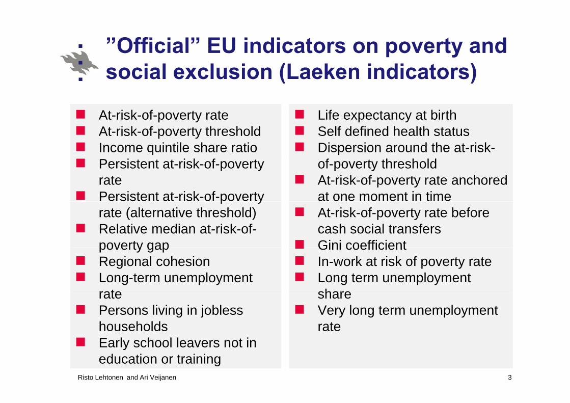
”Official” EU indicators on poverty and i l l i (L k i di t )social exclusion (Laeken indicators)

A i k f Lif bi hAt-risk-of-poverty rate At-risk-of-poverty threshold Income quintile share ratio

Life expectancy at birth Self defined health status Dispersion around the at-risk-

Persistent at-risk-of-poverty rate Persistent at-risk-of-poverty

of-poverty threshold At-risk-of-poverty rate anchored at one moment in time p y

rate (alternative threshold) Relative median at-risk-of-poverty gap

At-risk-of-poverty rate before cash social transfers Gini coefficientpoverty gap

Regional cohesion Long-term unemployment rate

Gini coefficient In-work at risk of poverty rate Long term unemployment sharerate

Persons living in jobless households E l h l l t i

share Very long term unemployment rate

Early school leavers not in education or training

3Risto Lehtonen and Ari Veijanen

European Union Low income by age and genderLow income by age and gender All the graphs below use the main EU measure of low income, namely a household income below 60% of the contemporary, national, median household income before deducting housing costs. All household incomes are after taxes have been deducted and after adjustment ('equivalisation') for household size and composition. This level of income is referred to as 'the poverty line' as that is the term used for it by the EU It is the sameThis level of income is referred to as 'the poverty line' as that is the term used for it by the EU. It is the same measure of low income as that used in most of the UK-specific sections of this website except that it is before, rather than after, deducting housing costs. To improve its statistical reliability given small sample sizes, the data in all the graphs bar the first is the average for the latest three years.

4

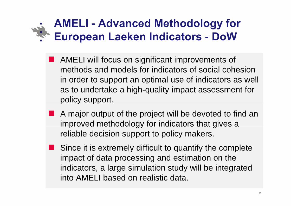
AMELI - Advanced Methodology for E L k I di t D WEuropean Laeken Indicators - DoW

AMELI will focus on significant improvements of methods and models for indicators of social cohesion in order to support an optimal use of indicators as wellin order to support an optimal use of indicators as well as to undertake a high-quality impact assessment for policy support. p y pp

A major output of the project will be devoted to find an improved methodology for indicators that gives aimproved methodology for indicators that gives a reliable decision support to policy makers.

Since it is extremely difficult to quantify the completeSince it is extremely difficult to quantify the complete impact of data processing and estimation on the indicators, a large simulation study will be integrated into AMELI based on realistic data.

5

AMELI - Advanced Methodology f E L k I di tfor European Laeken Indicators

AMELI (2008-2011) FP7 research project

ConsortiumUniversity of Trier (Coordinator)y ( )University of HelsinkiFHNW (Switzerland)Vienna University of TechnologyVienna University of TechnologyDestatis (Germany)Statistics AustriaStatistics FinlandStatistics FinlandSwiss Federal Statistical OfficeStatistics EstoniaSt ti ti l Offi f th R bli f Sl iStatistical Office of the Republic of Slovenia

6

P t i di t i AMELIPoverty indicators in AMELI

At-risk-of poverty rate

Quintile share ratio QSR (S20/S80 ratio)

Relative median at-risk-of poverty gap

Gini coefficientGini coefficient

7

8

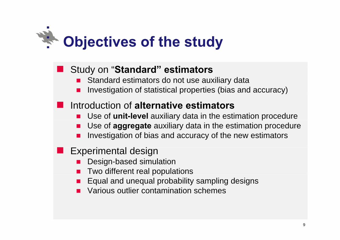
Obj ti f th t dObjectives of the study

Study on “Standard” estimatorsStandard estimators do not use auxiliary dataInvestigation of statistical properties (bias and accuracy)g p p ( y)

Introduction of alternative estimatorsUse of unit-level auxiliary data in the estimation procedurey pUse of aggregate auxiliary data in the estimation procedureInvestigation of bias and accuracy of the new estimators

E i l d iExperimental designDesign-based simulationTwo different real populationsp pEqual and unequal probability sampling designsVarious outlier contamination schemes

9

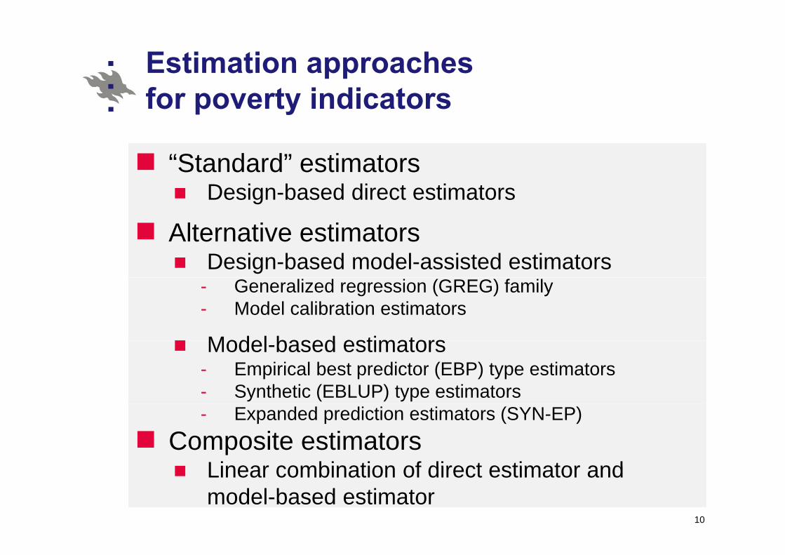
Estimation approaches f t i di tfor poverty indicators

“Standard” estimators Design-based direct estimators

Alternative estimatorsDesign-based model-assisted estimators

- Generalized regression (GREG) family- Model calibration estimators

Model based estimatorsModel-based estimators- Empirical best predictor (EBP) type estimators - Synthetic (EBLUP) type estimators- Expanded prediction estimators (SYN-EP)

Composite estimatorsLinear combination of direct estimator andLinear combination of direct estimator and model-based estimator

10

Modelling framework: GLMMModelling framework: GLMMGLMM formulation with area - specific random termsGLMM formulation with ( ) ( ( )), where m k k rr

E y f ′= +

area specific random termsu x β u

(.) refers to the chosen functional form refers to population unit

fk k U∈p p

refers to region (1

rr U U⊂

) ili i bl l′1 (1,k kx=x

0 1

,..., ) auxiliary variable values

( , ,..., ) fixed effects pk

p

x

β β β

′

′=β 0 1

0 ( ,..., ) area-spefic random effectsˆ

p

r r pru u ′=u

ˆ ˆPredictions: ( ( )), k k ry f k U′= + ∈x β u11

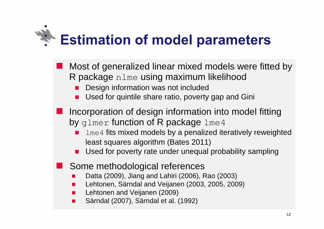
E ti ti f d l tEstimation of model parameters

Most of generalized linear mixed models were fitted by R package nlme using maximum likelihood

Design information was not includedDesign information was not includedUsed for quintile share ratio, poverty gap and Gini

Incorporation of design information into model fittingIncorporation of design information into model fitting by glmer function of R package lme4

lme4 fits mixed models by a penalized iteratively reweighted l t l ith (B t 2011)least squares algorithm (Bates 2011)Used for poverty rate under unequal probability sampling

Some methodological referencesSome methodological referencesDatta (2009), Jiang and Lahiri (2006), Rao (2003)Lehtonen, Särndal and Veijanen (2003, 2005, 2009)Lehtonen and Veijanen (2009)Lehtonen and Veijanen (2009)Särndal (2007), Särndal et al. (1992)

12

O tli t i ti hOutlier contamination schemes

Outlying mechanismsOCAR - Outlying completely at random

OAR - Outlying at random

Contamination modelsContamination modelsCCAR - Contamination completely at randomCAR Contamination at randomCAR - Contamination at randomNCAR - Contamination not at random

13

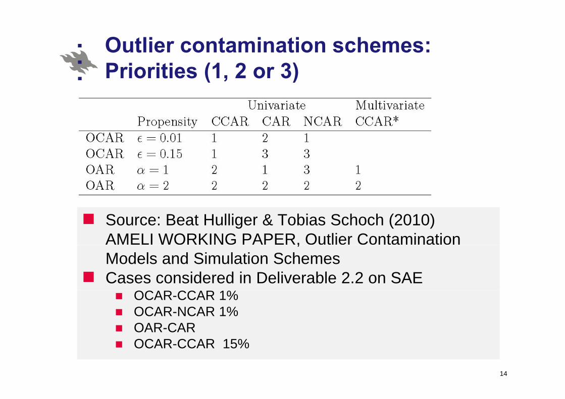
Outlier contamination schemes: P i iti (1 2 3)Priorities (1, 2 or 3)

Source: Beat Hulliger & Tobias Schoch (2010) AMELI WORKING PAPER, Outlier Contamination ,Models and Simulation Schemes Cases considered in Deliverable 2.2 on SAE

OCAR-CCAR 1%OCAR-NCAR 1%OAR-CAROCAR-CCAR 15%

14

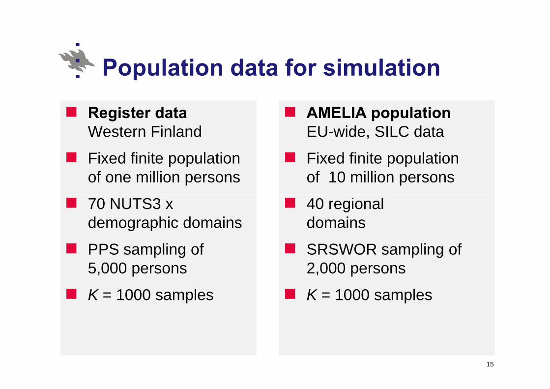
P l ti d t f i l tiPopulation data for simulation

Register data Western Finland

AMELIA populationEU-wide, SILC data

Fixed finite population of one million persons

Fixed finite population of 10 million persons

70 NUTS3 x demographic domains

40 regional domains

PPS sampling of 5,000 persons

SRSWOR sampling of 2,000 persons

K = 1000 samples K = 1000 samples

15

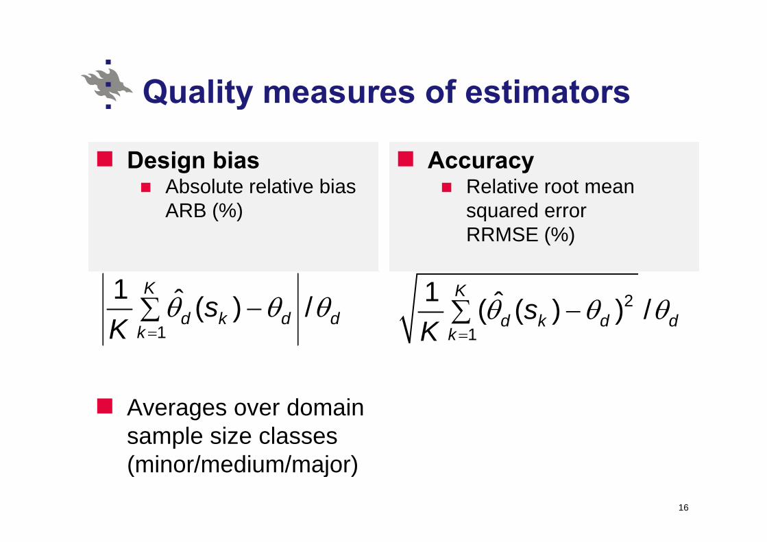
Quality measures of estimatorsQuality measures of estimators

Design biasAbsolute relative bias ARB (%)

AccuracyRelative root mean squared errorARB (%) squared error RRMSE (%)

θ θ θ=

−∑1

1 ˆ ( ) /K

d k d dk

sK

θ θ θ−∑ 2

1

1 ˆ( ( ) ) /K

d k d dk

sK=1kK =1kK

Averages over domain sample size classes ( i / di / j )(minor/medium/major)

16

Hi hli ht Quintile share ratioHighlights Quintile share ratioDirect (default) estimatorsI di t ti tPoverty rate

Direct (default)

Indirect estimatorsPrediction (synthetic) estimators SYN( )

estimatorsIndirect estimators

G li d i

Expanded prediction estimators SYN-EP

Composite estimatorsGeneralized regression MLGREGEmpirical Best Predictor

Composite estimatorsDefault with SYN-EP

Frequency-calibrated (EBP)

Modelling frameworkLogistic mixed models

predictorsModelling framework

Linear mixed modelsLogistic mixed models

Q: How to account for unequal probability

Linear mixed models

Q: Robustness against outlier contamination?q p y

sampling? outlier contamination?

17

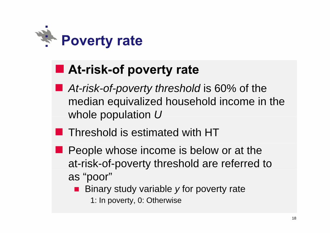
P t tPoverty rate

At-risk-of poverty rateAt-risk-of-poverty threshold is 60% of theAt risk of poverty threshold is 60% of the median equivalized household income in the whole population Uwhole population UThreshold is estimated with HTPeople whose income is below or at the at-risk-of-poverty threshold are referred to yas “poor”

Binary study variable y for poverty rate1: In poverty, 0: Otherwise

18

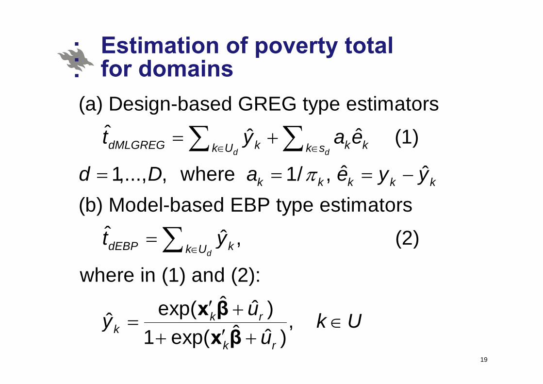
Estimation of poverty total f d ifor domains

(a) Design-based GREG type estimators(a) Design-based GREG type estimatorsˆ ˆˆ (1)dMLGREG k k kk U k st y a e

∈ ∈= +∑ ∑

ˆ ˆ1,..., , where 1/ , d d

dMLGREG k k kk U k s

k k k k kd D a e y yπ∈ ∈

= = = −

∑ ∑

(b) Model-based EBP type estimatorsˆ ˆ (2t y∑ ) , (2

ddEBP kk U

t y∈

= ∑ )

where in (1) and (2):where in (1) and (2): ˆ ˆexp( )ˆ k ruy k U′ +

= ∈x β , ˆ ˆ1 exp( )k

k r

y k Uu

= ∈′+ +x β

19

Estimation of poverty rate f d ifor domains

Estimator of at risk of poverty rateEstimator of at-risk-of poverty rateˆˆ = / dMLGREG dMLGREG dr t N

ordMLGREG dMLGREG d

ˆ ˆˆ = / ˆh 1/

dMLGREG dMLGREG dr t N

N ∑where , 1/d

d k k kk sN a a π

∈= =∑

ˆ similarly, 1,...,dEBPr d D=

20

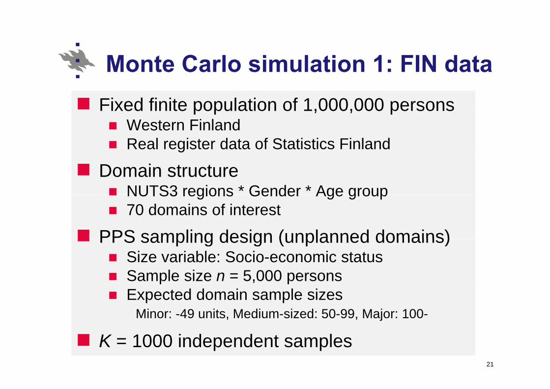
Monte Carlo simulation 1: FIN dataMonte Carlo simulation 1: FIN dataFixed finite population of 1 000 000 personsFixed finite population of 1,000,000 persons

Western FinlandReal register data of Statistics Finlandg

Domain structureNUTS3 regions * Gender * Age groupNUTS3 regions Gender Age group70 domains of interest

PPS sampling design (unplanned domains)PPS sampling design (unplanned domains)Size variable: Socio-economic statusSample size n = 5,000 personsp , pExpected domain sample sizes

Minor: -49 units, Medium-sized: 50-99, Major: 100-

K = 1000 independent samples 21

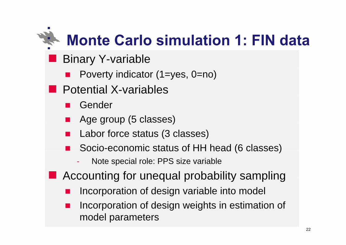
Monte Carlo simulation 1: FIN dataMonte Carlo simulation 1: FIN dataBinary Y-variable

Poverty indicator (1=yes, 0=no)Potential X-variables

GenderAge group (5 classes)ge g oup (5 c asses)Labor force status (3 classes) Socio-economic status of HH head (6 classes)Socio economic status of HH head (6 classes)

- Note special role: PPS size variable

Accounting for unequal probability samplingAccounting for unequal probability samplingIncorporation of design variable into modelIncorporation of design weights in estimation ofIncorporation of design weights in estimation of model parameters

22

Poverty rateEmpirical Best Predictor

23

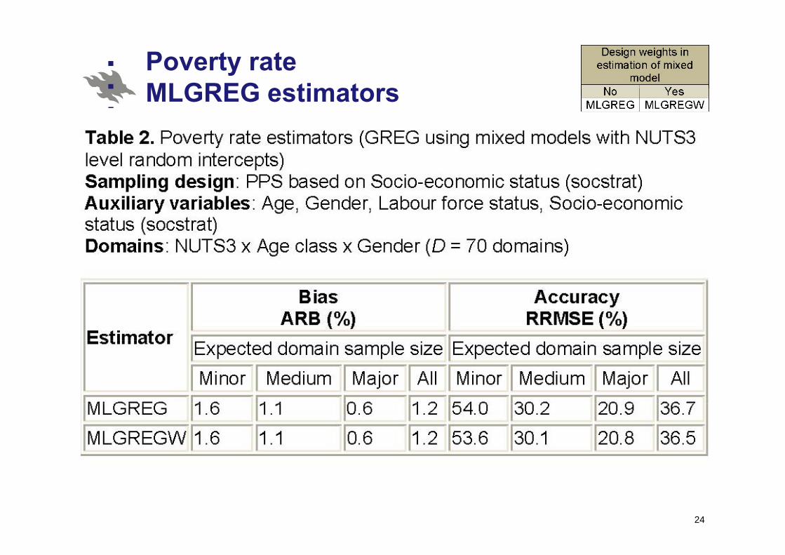
Poverty rate MLGREG estimatorsMLGREG estimators

24

Conclusions f t t

Model-based Empirical for poverty rate best predictor EBP

Design biased in all domain size classesModel-assisted GREG

Assisted by logistic mixed model

domain size classesLarge design bias in small domainsmixed model

Small design bias in all domain size classesG d i l

Good accuracy also in small domainsEBP gains much fromGood accuracy in large

domainsAccuracy can be poor

EBP gains much from inclusion of design informationAccuracy can be poor

in small domains

Poverty rate estimators are robust against outlierPoverty rate estimators are robust against outlier contamination (not shown here)Of the poverty rate estimators, EBP might be the best choice

25

Of the poverty rate estimators, EBP might be the best choice unless it is important to avoid design bias

Q i til h ti QSRQuintile share ratio QSR

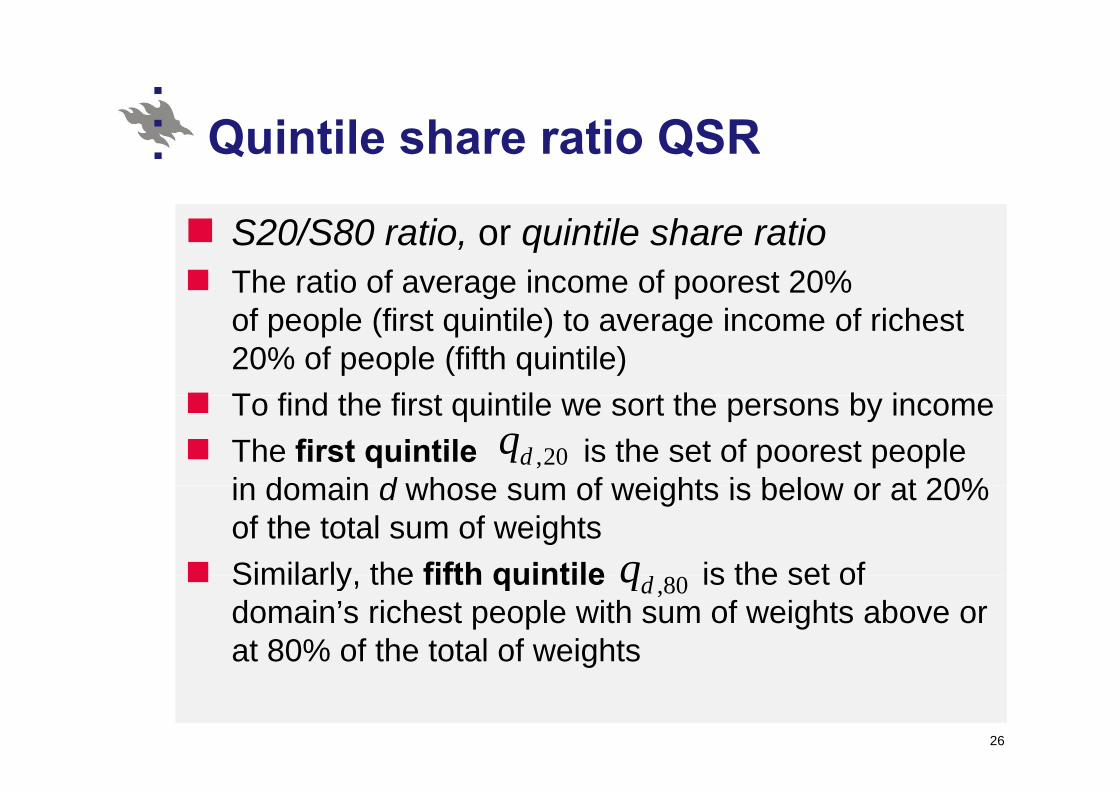
S20/S80 ratio, or quintile share ratioThe ratio of average income of poorest 20% of people (first quintile) to average income of richest 20% of people (fifth quintile)T fi d th fi t i til t th b iTo find the first quintile we sort the persons by incomeThe first quintile is the set of poorest people in domain d whose sum of weights is below or at 20%

,20dqin domain d whose sum of weights is below or at 20% of the total sum of weightsSimilarly the fifth quintile is the set ofqSimilarly, the fifth quintile is the set of domain’s richest people with sum of weights above or at 80% of the total of weights

,80dq

g

26

E ti ti h f QSREstimation approaches for QSR

Direct design-based estimatorUse of unit-level auxiliary dataUse o u t e e au a y data

Prediction estimators SYNExpanded prediction estimators SYN-EPComposite estimators COMP

Use of aggregate-level auxiliary datagg g yFrequency-calibrated predictors calculated using known domain marginal totals of auxiliary variablesC it ti t COMPComposite estimators COMP

Estimation under outlier contamination

27

Di t QSR ti tDirect QSR estimatorDirect estimator of first quintileDirect estimator of first quintile

ˆ 20 / , 1/d k k k k kS a y a a π= =∑ ∑,20 ,20

Direct estimator of fifth quintile d dk q k q∈ ∈

ˆ 80 /d k k kk q k q

S a y a∈ ∈

= ∑ ∑,80 ,80

Direct quintile share estimate in domaind dk q k q

d∈ ∈

ˆ2ˆ dSq =

0ˆ80

d

S28

80dS

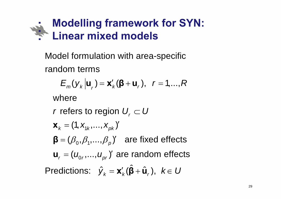
Modelling framework for SYN: Linear mixed models

Model formulation with area specificModel formulation with area-specific random terms ( ) ( ), 1,...,

wherem k k rr

E y r R′= + =u x β u where

refers to region (1 )

rr U U⊂′1

0 1

(1, ,..., )

( , ,..., ) are fixed effects k k pk

p

x x

β β β

′=

′=

xβ 0 1

0 ( ,...p

r ru=u , ) are random effectsˆˆ ˆ( )

pru ′

′ βˆ ˆPredictions: ( ), k k ry k U′= + ∈x β u29

S th ti QSR ti tSynthetic QSR estimatorQuintiles and are defined inq q; ,20 ; ,80Quintiles and are defined in population domain as if the weights were constant

SYN d SYN dq q

Synthetic estimator of first quintile ˆ ˆ20 / { }S I k∑ ∑

; ,20

; ,20 20 / { }

Fifth i tilSYN d d

dSYN k SYN dk q k U

S y I k q∈ ∈

= ∈∑ ∑i il lFifth quintile similarly

Synthetic quintile share estimator in domain dˆ20ˆ ˆ80

dSYNdSYN

SqS

=

30

80dSYNdSYNS

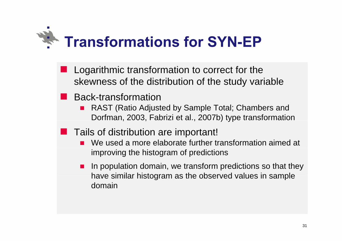
T f ti f SYN EPTransformations for SYN-EP

Logarithmic transformation to correct for the skewness of the distribution of the study variableBack-transformation

RAST (Ratio Adjusted by Sample Total; Chambers and Dorfman, 2003, Fabrizi et al., 2007b) type transformation, , , ) yp

Tails of distribution are important!We used a more elaborate further transformation aimed at improving the histogram of predictions

In population domain, we transform predictions so that they have similar histogram as the observed values in samplehave similar histogram as the observed values in sample domain

31

C it QSR ti tComposite QSR estimatorComposite quintile share estimator inComposite quintile share estimator in domain d

ˆ ˆˆ ˆ ˆ (1 )ˆ

dCOMP d d d dSYNq q qλ λ= + −ˆwhere is an average of

ˆ ˆ( )d

MSE q

λ

( ) ˆ ˆ ˆ ˆ( ) var( )dSYN

dSYN d

MSE qMSE q q+( ) ( )

over a domain size classdSYN dq q

32

Variance estimation for direct ti testimator

Estimation of ˆ ˆvar( )dq by bootstrap:Estimation of var( )dq by bootstrap: An artificial population is generated by cloning p p g y geach unit with frequency equal to the design weight Bootstrap samples are drawn with the original sampling design from the artificial populationsampling design from the artificial population The variance of the direct estimator is then estimated by the sample variance of estimates in the bootstrap samples

33

(Leiten and Traat 2006)

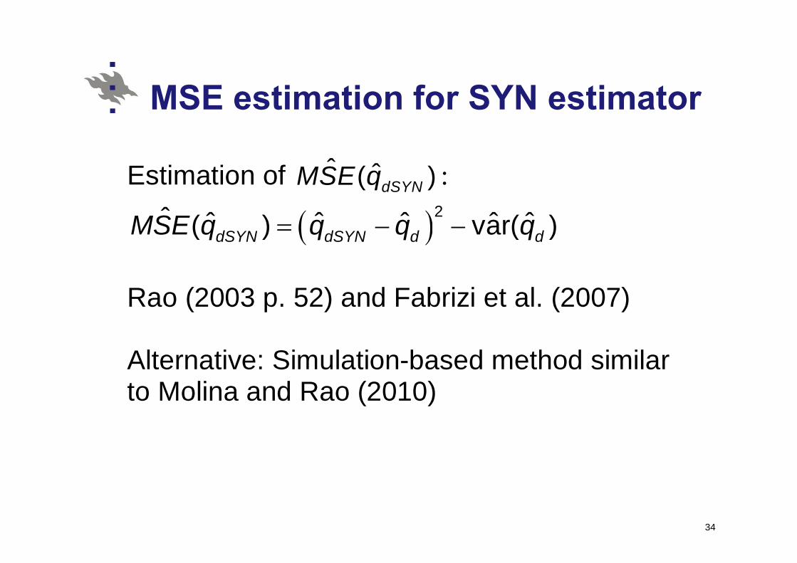
MSE ti ti f SYN ti tMSE estimation for SYN estimator

Estimation of ˆ ˆ( )dSYNMSE q :

( )2ˆ ˆ ˆ ˆ ˆ ˆ( ) ( )MSE ( )( ) var( )dSYN dSYN d dMSE q q q q= − − Rao (2003 p. 52) and Fabrizi et al. (2007) Alternative: Simulation-based method similar to Molina and Rao (2010)

34

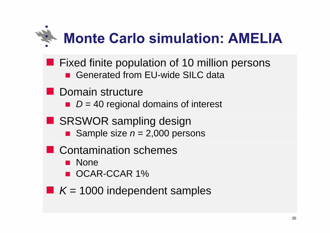
Monte Carlo simulation: AMELIAMonte Carlo simulation: AMELIAFixed finite population of 10 million personsFixed finite population of 10 million persons

Generated from EU-wide SILC data

Domain structureDomain structureD = 40 regional domains of interest

SRSWOR sampling designSample size n = 2,000 persons

Contamination schemesNoneOCAR-CCAR 1%

K = 1000 independent samples p p

35

Table 3. Quintile share estimators with linear mixed model fitted to log(income+1) including domain level random intercepts. Sampling design: SRSWORAuxiliary variables: Age and gender with interactions, education level, activity, degree of urbanisation D i R i l DIS i bl (40 d i )Domains: Regional DIS variable (40 domains)Contamination: None Data: AMELIA population

Estimator

Average ARB (%) Average RRMSE (%) Domain size class Domain size class

Minor20-49

Medium50-99

Major 100-

Minor20-49

Medium50-99

Major100-

Unit-level auxiliary data Direct (default) 1.6 1.9 1.3 24.7 23.5 22.7 Indirect SYN 122.9 132.7 143.9 124.2 134.0 145.2Indirect SYN-EP 10.1 11.2 9.4 12.6 13.6 12.6 Composite 7.8 8.9 7.6 12.1 12.3 11.4Area-level auxiliary data Frequency calibration 10 5 12 2 11 8 17 2 17 9 17 5

36

Frequency calibration 10.5 12.2 11.8 17.2 17.9 17.5Composite 8.1 9.5 9.2 15.5 15.7 15.2

Table 4. Quintile share estimators with linear mixed model fitted to log(income+1) including domain level random intercepts. S li d i SRSWORSampling design: SRSWORAuxiliary variables: Age and gender with interactions, education level, activity, degree of urbanisation D i R i l DIS i bl (40 d i )Domains: Regional DIS variable (40 domains)Contamination: OCAR-CCAR (1%) Data: AMELIA population

Estimator

Average ARB (%) Average RRMSE (%) Domain size class Domain size class Estimator

Minor20-49

Medium50-99

Major 100-

Minor 20-49

Medium50-99

Major100-

Unit-level auxiliary dataUnit level auxiliary dataDirect (default) 13.7 13.8 15.0 28.0 26.9 26.5Indirect SYN-EP 10.8 10.5 7.1 12.9 12.8 10.1C it 8 6 7 3 3 8 13 6 12 0 9 1Composite 8.6 7.3 3.8 13.6 12.0 9.1Area-level auxiliary data Frequency calibration 9.9 10.6 8.0 26.6 28.1 20.9

37 Composite 8.0 7.1 4.1 16.8 15.8 12.7

Conclusions f QSRfor QSR Expanded prediction

SYN-EPDefault estimator

No contamination: Small design bias

Some bias in all domain size classesSmall design bias

Large variance

O li i i

Much better accuracy than the default estimator in all domainOutlier contamination:

Substantial biasLarge variance

estimator in all domain size classesRobust against outlier Large variance contamination

Composite estimatorComposite estimatorOffers a reasonable compromise with respect to bias and accuracy

38

y

39

40

Thank you for yourThank you for your attention!attention!

41