March 15, 2012

Censuses and Surveys of Governments:  A Workshop on 

the Research and Methodology behind the Estimates 

Small Area Estimation for

Government Surveys  

 

Bac Tran and Carma Hogue 

 

Small Area Estimation for Government Surveys

Bac Tran Bac.Tran@census.gov

Carma Hogue Carma.Ray.Hogue@census.gov

Governments Division U.S. Census Bureau1, Washington, D.C. 20233-0001

Abstract: In the past three years, we developed decision-based estimation to estimate survey totals for the Annual Survey of Public Employment and Payroll (ASPEP). Recently, we developed a step-wise ratio method to estimate the Annual Finance Survey (AFS) characteristics of interest: Revenue, Expenditure, Debt, and Asset. In this paper, we discuss some small area challenges when we estimate survey totals at a function level, where the small area issue occurs. First, we introduce the idea of using synthetic estimation and modified direct estimation in ASPEP. Then, we modify the composite estimator as a weighted average of the modified direct estimator and synthetic estimator. We also apply the empirical Bayes to estimate the survey total, and then compare it to the modified composite using 2007 Census of Governments data. Secondly, we introduce the idea of using a step-wise ratio in the AFS with a validation the from New York census data. Lastly, we used the decision-based method to produce the state and nation total to compare with the step-wise ratio.

Key Words: Decision-based Estimation, Modified Direct Estimator, Synthetic Estimation, Composite Estimation, Step-Wise Ratio I. Introduction In survey analysis it is common to have a problem of small sample size, or an area where there were no sampled units. A direct estimator like Horvitz-Thompson estimator does not work well in very detailed categories areas with a small sample size or no sampled units. Small area issues can appear from other aspects like the ones in our government surveys: Annual Survey of Public Employment and Payroll (ASPEP), and Annual Finance Survey (AFS). Those two surveys use similar sample design. The sampled units were stratified by state and type of government for major variable aggregates (see below). However, in publication it was required that more detailed items are estimated (by function) (see below). This leads to Small Area Estimation (SAE) challenges. We describe briefly ASPEP and AFS characteristics below. The Annual Survey of Public Employment and Payroll (ASPEP) produces statistics on the number of federal, state, and local government employees and their gross payrolls. For more information on the survey, please see the Website for ASPEP http://www.census.gov/govs/apes/. ASPEP provides current estimates for full-time and part-time state and local government employment and payroll by government function (i.e., elementary and secondary education, higher education, police protection, fire

1 Disclaimer: This report is released to inform interested parties of research and to encourage discussion of work in progress. The views expressed are those of the authors and not necessarily those of the U.S. Census Bureau.

protection, financial administration, judicial and legal, etc.). ASPEP covers all states and local governments in the United States, which include counties, cities, townships, special districts, and school districts. The first three types of government are referred to as general-purpose governments, because they generally provide multiple government activities. Activities are coded as function codes. School districts cover only education functions. Special districts usually provide only one function, but can provide two or three functions. ASPEP is the only source of public employment data by program function and selected job category. Data on employment include number of full-time and part-time employees, gross pay, and hours paid for part-time employees. Reported data are for the government’s pay period that includes March 12. Data collection begins in March and continues for about seven months. The sample was augmented by births between 2007 and 2009. There are 89,526 state and local government units in the ASPEP universe. In 2009, after exploring possible cut-off sample methods for ASPEP, we developed a new modified cut-off sample method based on the current systematic stratified probability proportional-to-size (PPS) sample design. This method reduced the sample size, which saved resources, improved the precision of the estimates, reduced respondent burden, and improved data quality. The modified cut-off sample method was applied in two stages. We first selected a state-by-governmental type stratified PPS sample. The PPS sample was based on total payroll, which was the sum of full-time pay and part-time pay, from the Employment portion of the 2007 Census of Government. In the second stage, we constructed a cut-off point to distinguish small and large government units in the stratum. Lastly, we sub-sampled the strata with small-size government units with a simple random sampling method. ASPEP was designed to estimate survey totals of key variables: full-time employment, full-time payroll, part-time employment, part-time payroll, part-time hours, full-time equivalent employment, total payroll, and total employment. Cheng et al. (2009) proposed a method, Decision-based, to improve the precision of estimates and reduce the mean square error of weighted survey total estimates. Basically, the Decision-based method combined the strata to improve the models by testing the equality of the slopes of regression models from different strata. In Cheng et al. (2009), the hypothesis test was carried out in two steps. First, a test was performed of the null hypothesis that the slopes were identical. If the p-value was less than 0.05, the null hypothesis would be rejected to conclude that the regression lines were significantly different. In this case, there was no reason to compare the intercepts. If the p-value was greater than 0.05, the null hypothesis of equality of slopes could not be rejected, but intercepts could be compared. If the regression lines for the two substrata were not found to be significantly different, then a single line was estimated from the combined substrata. The Decision-based estimates provided a fundamental base to improve the reliability of the indirect small area estimation. As mentioned earlier ASPEP’s sampled units were stratified by state and government type. However, it was required to estimate the variables of interest at the state and function code level, which contained up to 30 categories for each government unit. This naturally brought the small area challenges, because we did not have any control on the sample size at the state and function code level. For example, the sample size for the state of Maryland was 48. But, there were only 3 sample units with the airport activity, labeled as function code of 001. In the worst case, we have no sample for some specific function codes. If there were missing data in some specific function for a government

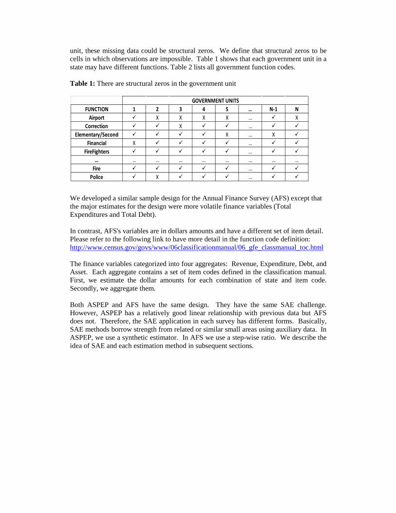
unit, these missing data could be structural zeros. We define that structural zeros to be cells in which observations are impossible. Table 1 shows that each government unit in a state may have different functions. Table 2 lists all government function codes. Table 1: There are structural zeros in the government unit

FUNCTION 1 2 3 4 5 … N-1 NAirport X X X X … X

Correction X … Elementary/Second X … X

Financial X … FireFighters …

… … … … … … … … …Fire …

Police X …

GOVERNMENT UNITS We developed a similar sample design for the Annual Finance Survey (AFS) except that the major estimates for the design were more volatile finance variables (Total Expenditures and Total Debt). In contrast, AFS's variables are in dollars amounts and have a different set of item detail. Please refer to the following link to have more detail in the function code definition: http://www.census.gov/govs/www/06classificationmanual/06_gfe_classmanual_toc.html The finance variables categorized into four aggregates: Revenue, Expenditure, Debt, and Asset. Each aggregate contains a set of item codes defined in the classification manual. First, we estimate the dollar amounts for each combination of state and item code. Secondly, we aggregate them. Both ASPEP and AFS have the same design. They have the same SAE challenge. However, ASPEP has a relatively good linear relationship with previous data but AFS does not. Therefore, the SAE application in each survey has different forms. Basically, SAE methods borrow strength from related or similar small areas using auxiliary data. In ASPEP, we use a synthetic estimator. In AFS we use a step-wise ratio. We describe the idea of SAE and each estimation method in subsequent sections.

Table 2: Function codes in the Annual Survey of Public Employment and Payroll ItemCode Meaning 000 Totals for Government 001 Airports 002 Space Research & Technology (Federal) 005 Correction 006 National Defense and International Relations (Federal) 012 Elementary and Secondary - Instruction 112 Elementary and Secondary - Other Total 014 Postal Service (Federal) 016 Higher Education - Other 018 Higher Education - Instructional 021 Other Education (state) 022 Social Insurance Administration (state) 023 Financial Administration 024 Firefighters 124 Fire - Other 025 Judicial and Legal 029 Other Government Administration 032 Health 040 Hospitals 044 Streets & Highways 050 Housing & Community Development (Local) 052 Local Libraries 059 Natural Resources 061 Parks & Recreations 062 Police Protection - Officers 162 Police - Other 079 Welfare 080 Sewerage 081 Solid Waste Management 087 Water Transport & Terminals 089 Other & Unallocable 090 Liquor Stores (state) 091 Water Supply 092 Electric Power 093 Gas Supply 094 Transit

II. Methodology What is small area estimation? Traditionally, small area is a small geographic area within a larger geographic area or a small demographic group within a larger demographic group. The sample size in the domain of interest is too small to use a standard estimator. For surveys of governments, small area refers to their state by function or itemcode. Most small area estimation methods borrow strength from related or similar areas using auxiliary data. There is growing demand from the public for reliable small area statistics. At the design stage, we can’t consider attaining precision at the state and function code level because it would force the sample to be too large. However, we have to handle this challenge at the estimation stage. II.A 2009 Annual Survey of Public Employment and Payroll Let g represent the state and f represent the function code. We want to estimate the total of employees or payroll information at the state by function level: gf

gf gfii U

Y Y∈

= ∑

where U is the universe of function codes in all states, and Ugf is the universe of

function code f, state

𝑛

𝑓

g. Thus, Ugf is a subset of U, that is, . The sample size

for function code f, , is less than or equal to the sample size n𝑔𝑓

, that is, n nf

domain of sample for function code f of state g is the intersection of the samplof state g and the universe of function code f and state g, . 𝑆𝑔𝑓 = 𝑆𝑔 ∩ 𝑈𝑔𝑓

≤ . The

𝑈 ⊂ 𝑈

e domain

In some cases, the changes in Employment statistics are relatively stable. Therefore, a linear regression is suitable for some state by government type cells as done prior to Fiscal Year (FY) 2009. However, due to small sample sizes and poor fit for many cells, a small area estimation method (SAE) is more appropriate. SAE is only applied for the PPS sample. For certainties, the direct estimate was used. Information on birth units is not available at the sampling stage. Therefore, we sample births separately from the PPS and certainties sample. Figure 1 briefly shows how we estimated the variable of interest in each cell of state by function code table. We applied the design-based direct estimator (Horvitz-Thompson), and the synthetic estimator in each cell. The direct estimator has high variability due to the small sizes. On the other hand the synthetic estimator reduces the variability but introduces some bias. Therefore, we introduce the composite estimator, which is a weighted average of those two estimators. We also modified the direct estimator (modified direct) by borrowing strength from similar cells to smooth the direct estimator. We will go through each of our estimators in detail in subsequent sections. In this

𝑌 s𝑔𝑓

ection, we discuss how to estimate 𝑌𝑔𝑓 for a given state g and function code f. Here, represents the survey total of key variables: full-time employment, full-time payroll, part-time employment, part-time payroll, part-time hours, full-time equivalent employment, total payroll, and total employment. We describe all the estimators used in our estimation process: Direct (Horvitz-Thompson), Decision-based, Synthetic, Composite, Modified Direct, and the Composite estimator.

II.A.1 Direct estimator (Horvitz-Thompson) A general design-based direct estimator for the total is:

y g, , , .f i gf i gfi S

t w y∈

=∑ (1)

where the weight, w ,,

1i gf

i gfπ= , and isf the inclu,i gπ sion probability for unit i in state

g and function code f. In this paper, we also denote ,y gft as ˆ HTgfY .

II.A.2 Decision-based estimator The Decision-based (DB) method helps to estimate the synthetic in each cell by providing a stable state total as a reliable estimator in a large area covering all small areas, states by function code level. In other words it was used for estimating the aggregates. DB was a process of testing the possibility of combining the strata in other to get a better estimate of the total. This method strengthened the statistical models for the area of estimation. The state total was estimated by a single stratum weighted regression (GREG) estimator specified as follows:

𝑦,𝐺𝑅𝐸𝐺 𝑦,𝜋 𝑥 𝑥,𝜋 𝑡 = 𝑡 + 𝑏�(𝑡 − 𝑡 )

(2)

where 𝑡𝑥 = ∑ 𝑥𝑖𝑖∈𝑈 , ,ˆ ix

i S i

xt π π∈

=∑ , ,ˆ iy

i S i

yt π π∈

=∑ , 2

( )( )ˆ

( )

i i ii S

i ii S

x x y yb

x x

π

π∈

∈

− −=

−

∑∑

,

where iπ is the inclusion probability, and ix is the auxiliary data from the Employment portion of the Census of Governments for government unit i. The slope b was obtained by the Decision-based (DB) process proposed by Cheng et al. (2009). The DB method improved the precision of estimates and reduced the mean square error of weighted survey total estimates. The idea was to test the equality of linear regression lines to determine whether we can combine data in different substrata. The null hypothesis 210 : bbH = , that is, the equality of the frame population regression

slopes for two substrata. In large samples, b is approximately normally distributed, ˆ ~ ( , )b N b ∑ . Under the null hypothesis, with two sub-strata 1U , 2U (large and small)

from samples 1S , 2S of sizes 1n and 2n , we have 1,21 2ˆ ˆ ~ (0, )b b N ∑−

where

1 21 2) )ˆ ˆ~ ( , , ~ ( ,b N b b N b∑ ∑ , and 1,2 1 2∑ = ∑ +∑ . Therefore, the test statistic is

1 2

1 2 1,2 1 2 1ˆ ˆ ˆ ˆ( ) ( ) ~b b b b χ−− ∑ − (3)

Our research showed that it was unnecessary to test the hypothesis for the intercept equality because our data analysis showed that we never rejected the null hypothesis of equality of intercepts when we could not reject the null hypothesis of equality of slopes. The critical value for a test based on (3) was obtained from a chi-squared distribution with 1 degree of freedom. The test was performed with a significance level of α = 0.05. If we could not reject the null hypothesis, then the slopes estimated in sub-strata 1S and

2S were accepted as the same, and the Decision-based estimator was equal to the GREG estimator for the union of two sample sets, that is, for 21 SSS ∪= . Otherwise, the Decision-based estimator would be the sum of two separate GREG estimators of stratum totals, that is,

,

2,

,1

ˆˆ

ˆ

y greg

y DB hy greg

h

tt

t=

= ∑ (4)

where ,y gregt denotes the GREG estimator from the combined stratum S, while ,ˆh

y gregt

denotes the GREG estimator from substratum h from sample hS . DB produced 51 (50 states and Washington D.C.) totals for each key variable. II.A.3 Synthetic estimation Synthetic estimation assumes that small areas have the same characteristics as large areas, and there is a reliable estimate for large areas. There are many advantages of synthetic estimation. They are accurate, simple and intuitive, aggregated estimates, that can be applied to all sample designs, and borrow strength from similar small areas. Synthetic estimation can even provide estimates for areas with no sample from the sample survey, and it does not need a study model.

if H0 is accepted

if H0 is rejected.

The general idea for synthetic estimation is that if we have a reliable estimate for a large area and this large area covers many small areas, then we can use this estimate to produce an estimate for a small area. The key element for calculating the synthetic estimation for a small area (state by function code level) is to estimate the proportion of that small area of interest within the large state area. This estimate for the small area is known as the synthetic estimate. The synthetic estimator for function code f of state g is: (5) where 𝑥𝑔𝑓 is the auxiliary information which is obtained from the Employment portion of

Census of Government and the state total, ˆDBgt is obtained by the Decision-based

estimate from equation (4).

II.A.4 Composite estimator In general, the synthetic estimator is a bias estimator. To balance the potential bias of the synthetic estimator, ˆ S

gfY , against the instability of the design-based direct estimator, ˆ HTgfY

we introduce a composite estimator as a weighted average of these two estimators. Thus, the composite estimate was applied on the PPS sample for each state by function code cell. Generally, it has the form:

.ˆ ˆ ˆ(1 )g gC HT Sgf gf gfY Y Yφ φ= + − (6)

where 2

ˆvar( )ˆ 1ˆ ˆ( )

f

f

HTgf

g S HTgf gf

yy y

φ = −−

∑∑

(Purcell & Kish, 1979). In some cases, we observed

negative φ . To fix this problem, we applied the method which was introduced by Lahiri and Pramanik (2010).

II.A.5 Modified direct estimator

We replaced the direct ˆ HTgfY in (6) by a modified direct estimate (MD), ˆ MD

gfY , due to instability of the design-based direct estimate caused by small sizes. The modified direct estimator from Rao’s Small Area Estimation (2003) is given as: (7)

ˆ ˆDBgf

gf

Sggf

f

Yx tx=∑

ˆˆ ˆ ˆ( )HT HTMDfY Y b X Xgf gf gf gfπ π= + −

where

ˆ, ,ˆ HT HT gfigf

i Sgf gigfgf

gfigf gf gfi

i Ugii S

xX

yY X x ππ ππ ∈∈∈

== = ∑∑ ∑ , and

,2

,

ˆ( )( ) /ˆ

( ) /gf

gf

gfi f gfi f gig G i S

fgfi f gi

g G i S

x x y yb

x x

π

π∈ ∈

∈ ∈

− −

=−

∑

∑

Since the modified direct estimators use data from outside the domain, we can see that the MD method is smoothed by borrowing strength across the state by using the census

year data, X. The estimator ˆ MDgfY

is approximately unbiased as the overall sample size

increases, even if the domain sample size is still small. The modified direct estimator (7)

is performed under some conditions which allowed producing a reliable ˆfb , for example,

goodness of fit 2R , slopes, and the sample sizes. II.A.6 Modified composite estimator With the MD estimator available, we can modify the composite estimator as: (8) We can re-write the MD estimator as: (9) where The first term ˆ

gf fX b is the synthetic regression estimator and the second term,Sgf

j jj

w e∈∑

approximately corrects the bias of the synthetic estimator. Figure 2 shows all the estimators we discuss in this paper.

( )ˆ ˆ ˆ1C MD Sgf gf g gfgy y yφ φ= + −

S

ˆˆ *gf

MDf j j

jY X b w egf gf

∈

= + ∑

ˆ*j j j fe y X b= −

` II.A.7 Variance Estimation The coefficient of variance, CV, is estimated by sqrt(𝑉𝑎𝑟� (𝑦�) )/𝑦� , where 𝑦� is the composite estimate from the PPS units, certainties, and births We applied a Taylor series method to estimate the approximate variance for the estimates derived in the previous section for each cell. For composite estimation, we estimate the mean square errors instead of approximate variance because of the bias from the synthetic estimation. We estimate the variance of the direct (Horvitz-Thompson) estimates and mean square error of the synthetic estimates, and then the mean square errors of the composite estimation is as follows:

𝑀𝑆𝐸� (𝑦�𝐶) = 𝜙2𝑣𝑎𝑟� (𝑦�𝐻𝑇) + (1 −𝜙)2𝑀𝑆𝐸� (𝑦�𝑆) For simplicity, we assumed there was no correlation between the design-based direct estimate and the synthetic estimate. Note: DC and Hawaii had CV = 0 because they are censuses.

II.B.1 2009 Annual Finance Survey- Step-wise Ratio AFS provides statistics on four categories: Revenue, Expenditure, Debt, and Asset (cash and security holdings). There are statistics for the 50 states areas and the District of Columbia, as well as a national summary. Statistics also are available by level of government: state, local, and state plus local aggregate. As in ASPEP, AFS uses the modified cut-off sampling method on stratified PPS units (see I.). The size is the maximum of dollar amounts among the four categories. Like ASPEP, sampled units in AFS are stratified by state and type but the reported aggregates are for state by item codes. For more information on the survey, please see the Website for ASPEP http://www.census.gov/govs/classification/index.html. Figure 3 is a snapshot of revenues 2009- State and Local Finances Revenue Figure 3: 2009 State and Local Finances (Revenue)

1 Duplicative Intergovernmental transactions are excluded

We used the step-wise ratio method in the 2009 AFS estimation because the AFS does not have a good linear relationship with previous data; moreover some AFS data are quite volatile across years. We used three years of data (2007, 2008, and 2009) to construct the step-wise ratios. The step-wise ratios were constructed as follows:

08 07

08 07

08 07

08 07

08 08

07

0708

08 08(0708

08 07(

08 08

1 070808 07

08 08 08

07

\ )

\ )

07

ˆ_

ˆ

ˆ ˆ

/

/

i S U

i S U

i S UC

i S U

i S i S

i U

C

C

AVG R

w yR

w y

w yR R

w y

w y w

y N

∈ ∩

∈ ∩

∈ ∩

∈ ∩

∈ ∈

∈

=

= =

=

∑∑∑∑∑ ∑∑

08 09

08 09

08 09

08 09

09 09

08 08

09 09(0809

09 08(

09 09

209 08

09 09 09

08 08 08

\ )

\ )

0809

0809

ˆ

ˆ ˆ

ˆ_/

/

i S S

i S S

i S S

i S S

i S i S

i S i S

C

C

C

w yR

w y

w yR R

w y

w y wAVG R

w y w

∈ ∩

∈ ∩

∈ ∩

∈ ∩

∈ ∈

∈ ∈

=

= =

=

∑∑∑∑∑ ∑∑ ∑

where 08, 09S S are the samples in the year 2008 and 2009, 08 09\ , \S C and S C are the

samples without certainties. Each 1 2ˆ ˆ,R R has three versions. The final version is the one

closest to 1. The estimate of the variable of interest for state g and item code is:

1 2 2007ˆ ˆˆgfy R R y=

As we can see from the construction the step-wise ratios borrow the strength of previous year information. II.B.2 2009 Annual Finance Survey- Decision-based Estimate As mentioned in II.A.2 the Decision-based method combined small and large strata in one stratum if they passed the hypotheses test. With more data the combined stratum

would produce a better estimate. We applied the Decision-based method to AFS to obtain the state and national totals, then compared them to the one obtained from the step-wise ratio estimate. The Decision-based total is given by the formula (4). The result is shown in III.B. III. Results III.A 2009 Annual Survey of Public Employment and Payroll

The composite estimator was used to estimate the survey totals in each cell (state by function) of the ASPEP. As mentioned earlier, the composite estimator is the weighted average of the two estimators: the design-based and the synthetic. The composite balances out the instability of the unbiased due to small sample sizes with the synthetic quantity. The weight 𝜙 pulls the estimate to the design unbiased estimate when it has enough data, and towards the synthetic estimate when there is insufficient sample size in the small area (Rao, 2003).

By applying the methods described in Section 2, we created Table 3 which is a typical illustration of our data analysis. Table 3 is for the variable, Full-Time Equivalent Employment, in several randomly selected states. Those methods included a combination of Decision-based estimation and an application of a SAE method. The conclusions are as follows:

• When there were no observed sampled units, we used the synthetic estimate where the design-based direct estimates were not present. For example, there were no sampled units in higher education in Arkansas or Oklahoma, so we obtained a reasonable synthetic estimate.

• The synthetic estimates were stable in small size areas where the design-unbiased estimates were very volatile.

• The modified direct estimates were closer to the census values. • When the sample sizes were large enough, all the estimators performed well and

they were close to each other. • The composite using the modified direct estimator was close to the 2007 Census

values most often.

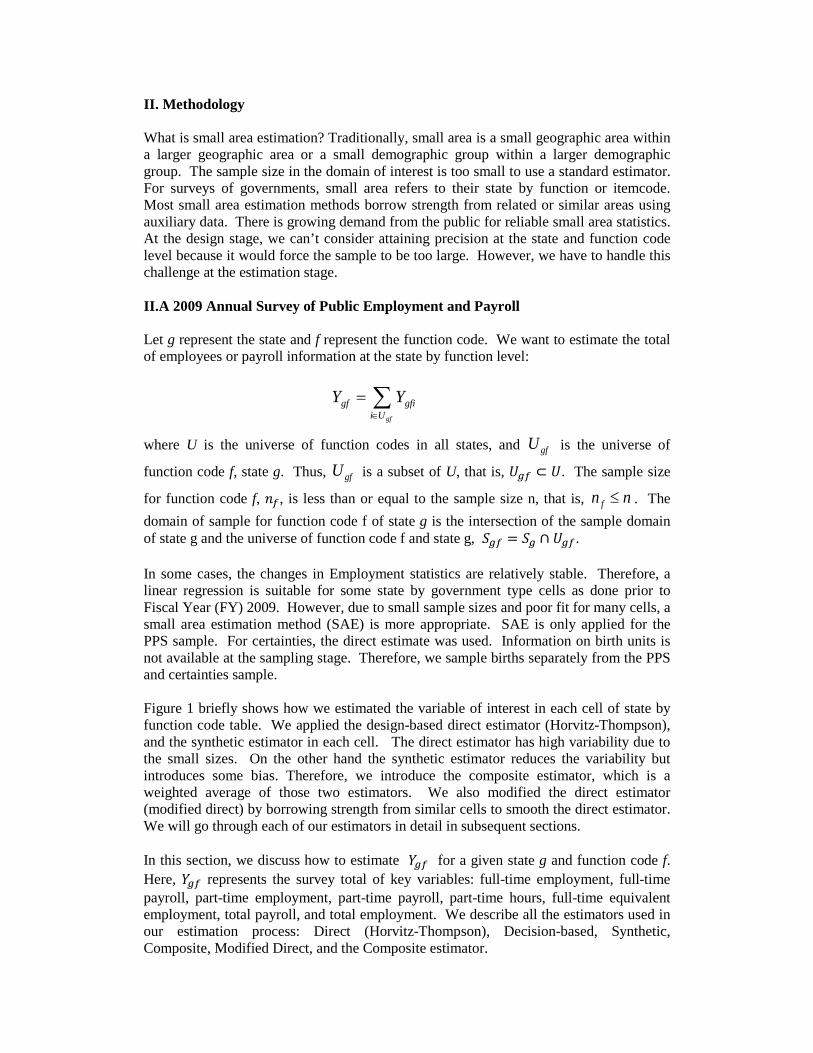
Figure 4 shows the comparison among the composite estimate, synthetic estimate, design-based direct estimate (Horvitz-Thompson), and the 2007 data for the variable, Full Time Employees, in Alabama for all functions from the most recent Census of Governments. Figure 5 is an enlargement from Figure 4 of itemcodes 080, 081, 089, 091, and 092. Figure 5 shows the performance of the synthetic and the composite over the design-based estimate. Figures 4 and 5 show that when the sample sizes are relatively small the synthetic and the composite estimates outperformed the design-based estimates.

Note: Codes 080 and 091 are sewerage and water supplies which are problematic because respondents cannot separate the data for the two variables. Code 089 is problematic because it is a catch-all "All other" variable, which tends to be volatile.

Table 3: Comparison of Different Estimators in Various Sample Sizes

Figure 4: Comparison of the Estimates from the Composite, Synthetic, and Horvitz- Thompson for the Variable Full-Time Employees in Alabama (all functions)

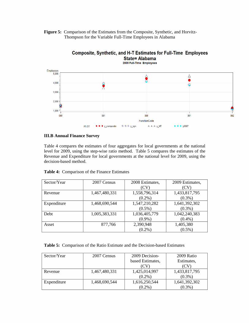
Figure 5: Comparison of the Estimates from the Composite, Synthetic, and Horvitz- Thompson for the Variable Full-Time Employees in Alabama

III.B Annual Finance Survey Table 4 compares the estimates of four aggregates for local governments at the national level for 2009, using the step-wise ratio method. Table 5 compares the estimates of the Revenue and Expenditure for local governments at the national level for 2009, using the decision-based method. Table 4: Comparison of the Finance Estimates Sector/Year 2007 Census 2008 Estimates,

(CV) 2009 Estimates,

(CV) Revenue 1,467,480,331 1,558,796,314

(0.2%) 1,433,817,795

(0.3%) Expenditure 1,468,690,544 1,547,210,282

(0.5%) 1,641,392,302

(0.3%) Debt 1,005,383,331 1,036,405,779

(0.9%) 1,042,240,383

(0.4%) Asset 877,766 2,390,948

(0.2%) 1,405,380

(0.5%) Table 5: Comparison of the Ratio Estimate and the Decision-based Estimates Sector/Year 2007 Census 2009 Decision-

based Estimates, (CV)

2009 Ratio Estimates,

(CV) Revenue 1,467,480,331 1,425,014,997

(0.2%) 1,433,817,795

(0.3%) Expenditure 1,468,690,544 1,616,250,544

(0.2%) 1,641,392,302

(0.3%)

As we can see the difference between the Decision-based and the step-wise ratio is 0.61% for Revenue, and 1.53% for Expenditure. This shows that the two different methods targeted the correct point of the estimate. We used New York 2009 census data to validate our estimation method. These data are available only for New York for a limited number of variables. The method yielded 89 percent of the cases where the step-wise ratio estimates are within 0.5 percent of the 2009 census. The cases out of 0.5 percent cut-off contained very volatile function codes like construction, or capital outlay. Those function codes represent the activities which are very difficult to model because the activities for those codes could be zero in one year but are active for the next year. If those activities are excluded in the estimation then the step-wise ratio estimates are within 0.5 percent of the 2009 New York census for 96.8 percent of the estimates. 6. Conclusions Bias of the synthetic estimator is the biggest disadvantage for synthetic estimation. Departures from the assumption may lead to large biases. Empirical studies have mixed results on the accuracy of synthetic estimators. The bias can not be estimated from the data. The variance estimator for the complicated composite estimator derived from a Decision-based method needs separate research which will be presented in a future paper. This paper presents two applications for the Decision-based and Small Area Estimation methods. They were applied to the estimation of Annual Survey of Public Employment and Payroll and the Annual Finance. SAE provides the composite estimate which smoothes the design unbiased estimators in small areas by introducing the synthetic term. The synthetic estimate is more reliable when derived from the Decision-based estimates. This property cannot be obtained from a simple regression synthetic. When these two methods are combined, we obtained better estimates than those of using direct estimators or with linear regression where the linear relationship is weak or even does not exist. As for AFS estimation with validation from the New York census data, the step-wise ratio is a good method to apply. This method also confirmed by the decision-based method (see II.B.2 and III.B) estimates which differed from those of the step-wise ratio with a very small margin. 7. Future Research We have some outstanding issues which need further research. We need to develop a simple and good variance estimator formula for the composite estimator other than a

resampling method. Regarding the weight, gφ , in the composite estimation method, we

replaced gφ = 0.5 when it was negative. Lahiri and Pramanik (2010) extended a method from Gonzalez & Waksberg (1973), which used the Average Design-based Mean

Squared Error (AMSE) to stabilize the gφ . We will apply this method in the future. We

will also explore in more detail the application of the Empirical Bayes method with an alternative assumption other than normality. Finally, we will apply this method to the Annual Finance Survey (AFS), as well as ASPEP. Acknowledgements We would like to thank Dr. Partha Lahiri from the University of Maryland at College Park and the Center for Statistical Research and Methodology of the Census Bureau for contributing ideas about average mean square errors and the bridge between composite estimation and the Empirical Bayes method. Also, we are indebted to our reviewer, Lisa Blumerman from the Governments Division of the Census Bureau. We also thank Dr. William Bell from the Associate Director of Research and Methodology of the Census Bureau for his valuable suggestions, which improved the original research. References Barth, J., Cheng, Y., Hogue, C. (2009). Reducing the Public Employment Survey Sample Size, JSM Proceedings. Cheng, Y., Corcoran, C., Barth, J., Hogue, C. (2009). An Estimation Procedure for the New Public Employment Survey, JSM Proceedings. Cheng, Y., Slud, E., Hogue, C. (2010). Variance Estimation for Decision-based Estimators with Application to the Annual Survey of Public Employment and, JSM Proceedings. Cochran, W.G. (1977), Sampling Techniques. Third Edition. New York: John Wiley & Sons, Inc. Deville, J-C. and Sarndal, C-E. (1992), Calibration Estimators in Survey Sampling, Journal of the American Statistical Association, Volume 87, Number 418, 376-382

Lahiri, P. and Pramanik, S. (2010b), Discussion of "Estimating Random Effects via Adjustment for Density Maximization" by C. Morris and R. Tang, Statistical Science, Volume 26, Number 2, 291-295

Lahiri, P. and Pramanik, S. (2010a), Estimation of Average Designed-based Mean Squared Error of Synthetic Small Area Estimators, Proceedings of statistics Canada Conference Purcell, N.J., and Kish, L. (1979), Estimates for Small Domain, Biometrics, 35, 365-384 Rao, J.N.K. (2003), Small Area Estimation, New York: John Wiley & Sons, Inc. Sarndal, C.-E., Swensson, B., and Wretman, J. (1992), Model Assisted Survey Sampling, Springer-Verlag.