sm.851-1 - sharing between the broadcasting service and the fixed
TRANSCRIPT

Recommendation ITU-R SM.851-1(04/1993)
Sharing between the broadcasting service and the fixed and/or mobile services
in the VHF and UHF bands
SM SeriesSpectrum management

ii Rec. ITU-R SM.851-1
Foreword
The role of the Radiocommunication Sector is to ensure the rational, equitable, efficient and economical use of the radio-frequency spectrum by all radiocommunication services, including satellite services, and carry out studies without limit of frequency range on the basis of which Recommendations are adopted.
The regulatory and policy functions of the Radiocommunication Sector are performed by World and Regional Radiocommunication Conferences and Radiocommunication Assemblies supported by Study Groups.
Policy on Intellectual Property Right (IPR)
ITU-R policy on IPR is described in the Common Patent Policy for ITU-T/ITU-R/ISO/IEC referenced in Annex 1 of Resolution ITU-R 1. Forms to be used for the submission of patent statements and licensing declarations by patent holders are available from http://www.itu.int/ITU-R/go/patents/en where the Guidelines for Implementation of the Common Patent Policy for ITU-T/ITU-R/ISO/IEC and the ITU-R patent information database can also be found.
Series of ITU-R Recommendations
(Also available online at http://www.itu.int/publ/R-REC/en)
Series Title
BO Satellite delivery
BR Recording for production, archival and play-out; film for television
BS Broadcasting service (sound)
BT Broadcasting service (television)
F Fixed service
M Mobile, radiodetermination, amateur and related satellite services
P Radiowave propagation
RA Radio astronomy
RS Remote sensing systems
S Fixed-satellite service
SA Space applications and meteorology
SF Frequency sharing and coordination between fixed-satellite and fixed service systems
SM Spectrum management
SNG Satellite news gathering
TF Time signals and frequency standards emissions
V Vocabulary and related subjects
Note: This ITU-R Recommendation was approved in English under the procedure detailed in Resolution ITU-R 1.
Electronic Publication Geneva, 2011
ITU 2011
All rights reserved. No part of this publication may be reproduced, by any means whatsoever, without written permission of ITU.

Rec. ITU-R SM.851-1 1
RECOMMENDATION ITU-R SM.851-1*
Sharing between the broadcasting service and the fixed and/or mobile services in the VHF and UHF bands
(1992-1993) Rec. ITU-R SM.851-1
The ITU Radiocommunication Assembly,
considering
a) that the World Administrative Radio Conference, (Geneva, 1979) (WARC-79), increased the number of frequency bands that might be shared between the broadcasting service and the fixed and mobile services;
b) that in many parts of the world, some bands are allocated, as specified in Article 5 of the Radio Regulations, to the fixed, mobile and broadcasting services on a co-primary basis;
c) that some administrations have partitioned the VHF and UHF bands between the three services and this situation has created some difficulty in coordination between two or more administrations which share borders in the coverage areas and which use these bands for different services;
d) that there is a requirement for standardized compatibility analysis procedures to facilitate the development of frequency assignment plans and equipment specifications applicable to national and multilateral arrangements;
e) that careful planning of frequency assignments to broadcasting, fixed and land mobile stations will lead to improvement in spectrum utilization by minimizing harmful interference to operations in the adjacent or shared frequency bands;
f) that fixed service applications in many parts of the world presently use the upper part of UHF television bands for radiotelephone links and are expected to remain for some time to come. However, new applications for those links in the fixed service are not expected to expand in these bands;
g) that fixed and mobile applications for services ancillary to broadcasting are likely to be expanded in the VHF and UHF bands;
h) that a variety of system characteristics exists for broadcasting, fixed and mobile service applications;
j) that studies are progressing in the Radiocommunication Sector (ITU-R) concerning the compatibility between the broadcasting service and the fixed and mobile services, in particular concerning systems involving new technology,
recommends
1. that frequency separation, geographical separation and time sharing, or a combination thereof, be used to ensure compatibility where sharing is required between different services. In this context, frequency sharing refers to the subdivision of the allocated bands between different services, geographical separation refers to the simultaneous use of a frequency by different services in separate geographical areas, and time sharing refers to the use of separate hours of operation for each of the services;
2. that the procedure in Annex 1 be used to determine the protection margin for the broadcasting service (sound and television) when it is operated simultaneously with either the fixed or land mobile service in shared or in adjacent VHF or UHF bands;
3. that the procedure in Annex 2 be used to determine the protection margin for the land mobile service when it is operated simultaneously with the broadcasting service in shared or in adjacent VHF or UHF bands;
_______________
* Radiocommunication Study Group 1 made editorial amendments to this Recommendation in 2011 in accordance with Resolution ITU-R 1-5..

2 Rec. ITU-R SM.851-1
4. that the procedure in Annex 3 be used to determine the protection margin for the fixed service when it is operated simultaneously with the broadcasting service in shared or in adjacent VHF or UHF bands;
5. that the system parameters related to determination of these protection margins include: minimum field strengths to be protected, protection ratios, antenna characteristics, propagation conditions and other related factors as described in Annexes 1, 2 and 3;
6. that the parameters contained in this Recommendation be used only for systems referred to in Annexes 1, 2 and 3;
7. that with the introduction of new technology (e.g. digital television, digital audio broadcasting, digital mobile and digital fixed) these parameters should be extended to accommodate future developments and to take account of ongoing Radiocommunication Sector (ITU-R) studies.
ANNEX 1
Protection of the broadcasting service from the fixed and land mobile services
PART I
TO ANNEX 1
Television services
1. Minimum field strength to be protected
Table 1 gives the minimum field strength values to be protected at 10 m above ground level for the broadcasting service (television) and the wanted field strength values from which they are derived.
TABLE 1
The field strength to be protected is derived from the wanted field strength by taking account of the need to protect 90% of locations and the relatively high man-made noise levels in the VHF bands.
Band I (41-68 MHz)
Band II (76-100 MHz)
Band III (162-230 MHz)
Band IV (470-582 MHz)
Band V (582-960 MHz)
Field strength to be protected (dB(μV/m)) at edge of coverage area (50% of time, 90% of locations)
46 48 49 53 58
Wanted field strength (dB(μV/m)) at edge of coverage area (50% of time, 50% of locations) from Recommendation ITU-R BT.417
48
52
55
65
70

Rec. ITU-R SM.851-1 3
However, the values given in Table 2 are used in North America for the wanted field strength at the edge of coverage area and for the field strength to be protected at 10 m above ground level (50% of time and 50% of locations in both cases).
TABLE 2
2. Protection ratios
2.1 General
Protection ratios for the various television systems are given in Recommendation ITU-R BT.655. The values shown in this Annex are based on these texts as well as on the new studies carried out by some administrations.
Protection ratios covering tropospheric (T) and continuous (C) interference are included, the values being applicable to interference produced by one single source. The ratios applied to tropospheric (T) interference correspond closely to a slightly annoying impairment condition (Grade 3). They are considered to be acceptable only if the interference occurs for a small percentage of the time, not precisely defined but generally considered to be between 1% and 10%. For substantially non-fading unwanted signals, it is necessary to provide a higher degree of protection. In this case, the protection ratios appropriate to continuous (C) interference, which corresponds closely to perceptible but not annoying (Grade 4), should be used. If the latter ratios are not known, then the tropospheric (T) values increased by 10 dB can be applied.
Within a television channel, the required protection ratios for the vision and the sound signals should be considered separately.
Protection ratio requirements, particularly in the out-of-channel range, can be significantly increased due to non-linear effects in the receiver brought about by high level single or multiple unwanted input signals. Studies have shown that values can increase by up to 25 dB.
2.2 Protection ratios for the vision channel
The unwanted signal can fall into any part of the vision channel, therefore the protection ratios for overlapping channels given in Figs. 1 to 3, and Tables 4 to 6 (taken from Recommendation ITU-R BT.655) should be applied.
All the protection ratio values in the figures and tables are relevant for the case of an unwanted CW signal or FM signal, falling into the vision channel, the wanted vision signal being negatively modulated.
The corrections which should be made for positively modulated wanted vision signals and for other types of potentially interfering signals are given in Table 3.
2.2.1 525-line systems
The protection ratio values to be applied for 525-line systems are given in Fig. 1 and Table 4 for tropospheric interference.
For continuous interference the values should be increased by 10 dB.
54-88 MHz 174-216 MHz 470-806 MHz
Wanted field strength and field strength to be protected (dB(μV/m)) at edge of coverage area (50% of time and 50% of locations)
47
56
64

4 Rec. ITU-R SM.851-1
TABLE 3
Correction values for different wanted and unwanted signals
FIGURE 1 et TABLEAU 4 [D01] = 9 cm
2.2.2 625-line systems
The protection ratio values to be applied for 625-line systems are given in Figs. 2 and 3, and Tables 5 and 6.
–3 –2 –1 0 1 2 3 4 5 6 7
0
10
20
30
40
50
60
FIGURE 1 and TABLE 4
525-line systems (M/NTSC and M/PAL) Tropospheric interferenceUnwanted signal: CW carrier
Pro
tect
ion
rati
o (d
B)
Frequency difference between unwanted and wanted carriers (MHz)
NTSC
PAL
Monochrome
D01
Unwanted signal Correction factors (dB)
Wanted signal CW FM AM
Vision signal negative modulated − 0 − 0 − 0
Vision signal positive modulated − 2 − 2 − 2
Frequency difference (MHz)
−1.5 −1.0 −0.75 0.3 1.0 2.5 3.0 3.5 3.7 4.1 4.5
NTSC (dB) 50 50 45
PAL (dB) 0 30 40 50 50 37 45 45 45 15
Monochrome (dB) 26 25 20

Rec. ITU-R SM.851-1 5
Figure 2 et TABLEAU 5 [D02] = 8 cm
(1) H, I, K1, L television systems.
(2) B, D, G, K television systems.
(3) B, G television systems: range is 5.3-6.0 MHz.
(4) This value is valid until the end of the channel.
(5) D/SECAM and K/SECAM: add 5 dB.
2.3 Protection ratios for the sound channel
2.3.1 Analogue sound systems (one or two-sound carrier systems)
Protection ratio values for analogue sound signals are given in Table 7.
In the case of a two-sound carrier system each sound carrier must be considered separately.
The maximum deviation of the wanted FM sound carrier is assumed to be 50 kHz. Corrections should be made for other deviations.
2.3.2 Digital sound systems
Some values for the protection of digital sound signals are given in Table 8.
2.4 Protection ratios for out-of-channel interference
2.4.1 Adjacent channels
2.4.1.1 525-line systems
The protection ratio values to be applied for 525-line systems are given in Figs. 4a and 4b and Table 9 for continuous and tropospheric interference.
–1 0 1 2 3 4 50
10
20
30
40
50
60
3 4 5 6 3 4 5 6
H, I, K1, L
B, D, G, K
FIGURE 2 and TABLE 5
625-line systemsTropospheric interference
Frequency difference between unwanted and wanted carriers (MHz)
SECAMPAL
Monochrome
D02
Luminance
Frequency difference between unwanted and wanted carriers (MHz)
Luminance range PAL SECAM
MHz −1.25 (1) −1.25 (2) −0.5 0.0 0.5 1.0 2.0 3.0 3.6-4.8 5.7-6.0 (3) (4) 3.6-4.3 (5) 5.7-6.3 (3) (4)
dB 32 23 44 47 50 50 44 36 45 25 40 25

6 Rec. ITU-R SM.851-1
Figure 3 et et TABLEAU 6 [D03] = 8.5 cm
(1) H, I, K1, L television systems.
(2) B, D, G, K television systems.
(3) B, G television systems: range is 5.3-6.0 MHz.
(4) This value is valid until the end of the channel.
(5) D/SECAM and K/SECAM: add 8 dB.
TABLE 7
Protection ratios for wanted analogue sound carriers of a television signal (dB) Unwanted signal: CW or FM sound carrier
–1 0 1 2 3 4 50
10
20
30
40
50
60
3 4 5 6 3 4 5 6
H, I, K1, L
B, D, G, K
–2
FIGURE 3 and TABLE 6
625-line systemsContinuous interference
Frequency difference between unwanted and wanted carriers (MHz)
SECAMPAL
D03
Luminance
Frequency difference between unwanted and wanted carriers (MHz)
Luminance range PAL SECAM
MHz −1.25 (1) −1.25 (2) −0.5 0.0 0.5 1.0 2.0 3.0 3.6-4.8 5.7-6.0 (3) (4) 3.6-4.3 (5) 5.7-6.3 (3) (4)
dB 40 32 50 54 58 58 54 44 53 35 45 30
Wanted sound signal
Difference between wanted sound carrier and unwanted carrier
Tropospheric interference Continuous interference
(kHz) FM AM FM AM
0 32 49 39 56
15 30 40 35 50
50 22 10 24 15
250 − 6 7 − 6 12

Rec. ITU-R SM.851-1 7
TABLE 8
Protection ratios for wanted digital sound carriers of a television signal (dB)
(No frequency separation)
(1) The values given incorporate an additional 6 dB safety margin to allow for the sudden onset of severe degradation of the digital sound system in the presence of interference. For the same reason, there is no difference between the protection ratios for tropospheric and continuous interference.
(2) Protection ratios for unwanted digital broadcasting signals (refer to Recommendation ITU-R BT.655).
Figure 4a [D04] = 11cm
FIGURE 4b...[D05] = 3 CM
7,25–7.25 –6.25 –5.25 –4.25 –3.25 –2.25 –1.25
20
10
0
–10
–20
–30
–40
FIGURE 4a
Protection ratios for the lower adjacent channel, NTSC/system M
Frequency difference (MHz)
Prot
ecti
on r
atio
(dB
)
Continuousinterference
Troposphericinterference
D04
7 ,2 5
FIGURE 4b
Protection ratios for the upper adjacent channel, NTSC/system M
Frequency difference (MHz)
Prot
ecti
on r
atio
(dB
)
Continuousinterference
Troposphericinterference
D05
4.75 5.75 6.75 7.75 8.75 9.75 10.75
20
10
0
–10
–20
–30
–40
Unwanted Wanted FM/CW (1) AM (1) Digital (2)
Digital T 12 11 12
C 12 11 12

8 Rec. ITU-R SM.851-1
TABLE 9
Protection ratios for the adjacent channels, 525-line NTSC systems
2.4.1.2 625-line systems
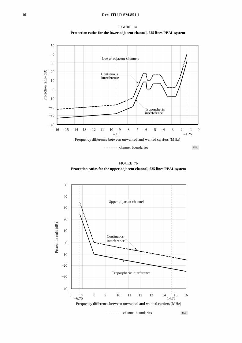
The protection ratio values to be applied for 625-line systems are given in Table 10 and in Figs. 5 and 6 for tropospheric and continuous interference. For system I/PAL the values for the lower adjacent channel are given in Fig. 7 and Table 11.
TABLE 10
Protection ratios for the adjacent channels, 625-line systems
Frequency difference Protection ratio (dB)
(MHz) Continuous Tropospheric
−7.25 −26 −36
−5.25 −15 −25
−3.52 −10 0
−2.25 3 −7
−1.25 20 10
−4.75 16 6
−5.75 5 −5
−6.75 −9 −19
−8.75 −22 −32
10.75 −30 −40
Frequency difference Protection ratio (dB)
(MHz) Continuous Tropospheric TV systems
−14.05 −10 −15 B, D, G, H, K, K1, L
1−6.05 −10 −15 B, D, G, H, K, K1, L
1−2.55 −−11 −1 B, D, G, H, K, K1, L
1−1.55 −11 −1 B, D, G, H, K, K1, L
1−1.25 −40 −32 H, K1, L
1−1.25 −32 −23 B, D, G, K
5.75 −30 −25 B, G, H/SECAM
5.75 −35 −25 B, G, H/PAL
6.25 −2 −12 B, G, H
6.75 −30 −25 L, D, K, K1/SECAM
8.55 −2 −12 L, D, K, K1/SECAM
15.05 −2 −12 B, D, G, H, K1, L

Rec. ITU-R SM.851-1 9
Figure 5 [D06] = 10 cm
Figure 6 [D07] = 10 cm
–15 –14 –13 –6 –5 –4 –3 –2 –1 0 5 6 7 8 9 10 11 15
–10
–20
0
10
20
30
40
50
H, K1, L
B, D, G, K
B, G, H
L, D, K, K1 / SECAM
FIGURE 5
Protection ratios for the adjacent channels, 625-line systemstropospheric interference
Pro
tect
ion
rati
o (d
B)
Frequency difference between unwanted and wanted carriers (MHz) D06
Lower adjacent channel Upper adjacent channel
–15 –14 –13 –6 –5 –4 –3 –2 –1 0 5 6 7 8 9 10 11 15
–10
–20
0
10
20
30
40
50
H, K1, L
B, D, G, K
B, G, H / PAL
L, D, K, K1 / SECAM
B, G, H / SECAM
FIGURE 6
Protection ratios for the adjacent channels, 625-line systemscontinuous interference
Pro
tect
ion
rati
o (d
B)
Frequency difference between unwanted and wanted carriers (MHz) D07
Lower adjacent channel Upper adjacent channel
10 Rec. ITU-R SM.851-1
Figure 7a [D08] = 11 cm
FIGURE 7b...[D09] = 3 CM
–16 –15 –14 –13 –12 –10 –9 –8 –7 –6 –5 –4 –3 –2 –1
–10
–20
0
10
20
30
40
50
–400–11
–30
–9.3 –1.25
D08
FIGURE 7a
Protection ratios for the lower adjacent channel, 625 lines I/PAL system
Frequency difference between unwanted and wanted carriers (MHz)
Prot
ecti
on r
atio
(dB
)
Lower adjacent channels
Continuousinterference
Troposphericinterference
channel boundaries
6 7 8 9 10 12 13 14 15 16
–10
–20
0
10
20
30
40
50
–40
11
–30
–6.75 14.75
D09
FIGURE 7b
Protection ratios for the upper adjacent channel, 625 lines I/PAL system
Frequency difference between unwanted and wanted carriers (MHz)
Prot
ecti
on r
atio
(dB
)
Upper adjacent channel
Tropospheric interference
channel boundaries
Continuousinterference

Rec. ITU-R SM.851-1 11
TABLE 11
Protection ratio for the adjacent channels, 625 lines I/PAL system
2.4.2 Image channels
The protection ratio required will depend on the intermediate frequency and image-channel rejection of the receiver, and on the type of unwanted signal falling in the image channel. It can be determined by subtracting the image rejection figure from the required protection ratio given in § 2.2 and 2.3 above.
Image-channel rejection:
systems D and K/SECAM : 45 dB (VHF) and 30 dB (UHF)
system D/PAL: 45 dB (VHF) and 40 dB (UHF)
system I: 50 dB (UHF)
system M (Japan): 60 dB (VHF) and 45 dB (UHF)
all other systems: 40 dB (UHF).
Frequency difference Protection ratio (dB)
(MHz) Continuous Tropospheric
−16.00 −23 −33
−9.30 −18 −28
−7.40 −10 −20
−6.50 11 1
−6.20 18 8
−5.90 18 8
−5.80 10 0
−5.40 10 0
−5.10 16 6
−5.00 16 6
−4.30 16 6
−4.00 12 2
−3.50 2 −8
−3.00 2 −8
−2.50 2 −8
−2.00 14 4
−1.25 40 32
+6.75 35 25
+8.00 0 −10
+10.00 −€4 −14
+14.75 −13 −23
+16.00 −15 −25

12 Rec. ITU-R SM.851-1
2.4.3 Other types of interference
In the out-of-channel range some specific frequencies, depending upon the technology used in the TV receiver, such as local oscillator frequency, IF spacing, half IF spacing, etc., may require higher values of protection ratio.
3. Protection margin for television services
The protection margin (PM) is given (dB) by:
PM = FS – combined value of (NF + AF) for all interfering sources
where:
FS : relevant field-strength value (dB(μV/m)) given in § 1 above
AF : adjustment factor (dB), intended to deal with antenna discrimination and clutter loss (see § 4.1)
NF : nuisance field and the larger of EC and ET given below (dB(μV/m)).
For continuous interference:
EC = E(50,50) + P + AC
For tropospheric interference:
ET = E(50,t) + P + AT
where:
E(50,t) : field strength (dB(μV/m)) of the interfering transmitter, normalized to 1 kW, and exceeded during t% of the time, determined using Recommendation ITU-R P.1546.
For tropospheric interference the value of t is between 1 and 10 (the precise value should be specified by each administration)
P : e.r.p. (dB(kW)) of the interfering transmitter
A : protection ratio (dB)
and where the indices C and T indicate continuous and tropospheric interference respectively.
The protection ratio for continuous interference is applicable when the resulting nuisance field is stronger than that resulting from tropospheric interference, that is, when:
EC > ET
This means that EC should be used in all cases when:
E(50,50) + AC > E(50,t) + AT
The calculated protection margin should be positive at all locations where a television service is required.
The combination of multiple interference from co-sited and non co-sited sources is discussed in § 4.2 and 4.3 below.
Information regarding fixed services or base stations of the land mobile service with effective antenna heights of less than 37.5 m is given in § 4.4 below.
4. Additional factors to be considered
4.1 Adjustment factors (AF)
Four distinct cases of interference to a station of the television service from stations of the fixed or land mobile services can be identified; these are dealt with separately below.
Rec. ITU-R SM.851-1 13
4.1.1 Interference from stations of the fixed service or base stations of the land mobile service which are orthogonally polarized with respect to a station of the television service
In this case, the adjustment factor is equal to the antenna discrimination which has a value of −16 dB for 50% of locations and −10 dB for 90% of locations.
4.1.2 Interference from stations of the fixed service or base stations of the land mobile service which have the same polarization as a station of the television service
In this case, the adjustment factor is equal to the relevant receiving antenna directivity discrimination value given in Recommendation ITU-R BT.419. For television Band II, the values as given for Band I should be used.
4.1.3 Interference from a land mobile station operating at more than 40 km outside the coverage area of a station of the television service
No polarization discrimination can be taken into account because:
– the mobile transmitter system, consisting of an antenna and the body of a vehicle, cannot be assumed to radiate with only horizontal or vertical polarization;
– the effect of environmental clutter near the mobile transmitter can be expected to introduce a degree of depolarization.
It would be impracticable to carry out calculations for all possible geographical locations for any mobile station, taking account of propagation losses and receiving antenna directivity discrimination. A reasonable simplification of the problem is to carry out interference calculations for the e.r.p. of the mobile station assuming this to be situated at the base station site with an effective antenna height of 75 m. It is then appropriate to use an adjustment factor of −15 dB (see Note 1) to allow for the effect of clutter loss and ground reflection effects near the mobile station.
In some cases, it may be possible to include an additional adjustment to allow for the directivity of the television receiving antenna, as given in Recommendation ITU-R BT.419. For television in Band II, the values given for Band I should be used.
Note 1 – See Final Acts of the Second Session of the Regional Administrative Conference for the planning of VHF/UHF Television Broadcasting in the African Broadcasting Area and Neighbouring Countries (RARC AFBC(2)).
4.1.4 Interference from a land mobile station operating less than 40 km from a receiving site of a station of the television service
In this case, it is necessary to carry out detailed calculations for individual, worst-case paths. No polarization discrimination can be taken into account, for the same reasons as are explained in § 4.1.3.
4.2 Multiple interference from co-sited sources
The interference arising from multiple co-sited sources should be combined by means of the power-sum method:
E = 10 log10
n
i = 1
10
Ei10
where:
Ei : value (dB(μV/m)), of (NF + AF) for each individual co-sited source. As indicated in § 3 NF is expressed in dB(μV/m) and AF in dB
n : number of co-sited sources
E : effective interference (dB(μV/m)).
Note 1 – The value of E represents one of the terms to be included in the procedure given in § 4.3 below.

14 Rec. ITU-R SM.851-1
4.3 Multiple interference from non co-sited sources
The interference arising from multiple non co-sited sources should be combined by using the simplified multiplication method given in Annex II of the Final Acts of the RARC AFBC(2), 1989, reproduced herein as Appendix 1 to Annex 1.
4.4 Effective transmitting antenna heights
The effective transmitting antenna height is determined according to Recommendation ITU-R P.1546.
When the effective transmitting antenna height is less than 37.5 m or more than 1 200 m, the field-strength values are calculated using the method described in the Final Acts of the RARC AFBC(2), reproduced herein as Appendix 2 to Annex 1.
5. Interference assessments
Interference assessments should normally be made for several reception points within the service area of the television transmitter. These points should be those which are considered to be most likely to suffer from interference.
Moreover, for rebroadcasting stations, it is necessary to ensure that the received television signal is also protected against interference. In this case, the protection ratios given in Recommendation ITU-R BT.655 for the limit of perceptibility are normally used.
PART II
TO ANNEX 1
Sound broadcasting services
1. Minimum field strengths to be protected
The minimum values of field strength which require protection from the fixed and mobile service as given in Recommendation ITU-R BS.412, are:
37 dB(μV/m) at an antenna height of 10 m above ground for monophonic reception
48 dB(μV/m) at an antenna height of 10 m above ground for stereophonic reception.
2. Protection ratios
The protection ratios for a wanted FM sound broadcasting station and an unwanted AM or FM fixed or mobile station are given in Figs. 8 and 9, and Tables 12 and 13 (for a maximum frequency deviation of ± 75 and ± 50 kHz respectively).
In the case of a very narrow-band FM interfering system, some relaxation may be possible (see also Report ITU-R SM.659).

Rec. ITU-R SM.851-1 15
Figure 8 [D10] = Pleine Page
60
50
40
30
20
10
0
–10
–20
S1
S2
M1
M2
0 100 200 300 400
FIGURE 8
Radio-frequency protection ratiosrequired by broadcasting services in band 8 (VHF)
at frequencies between 87.5 MHz and 108 MHzusing a maximum frequency deviation of ± 75 kHz
Rad
io-f
requ
ency
pro
tect
ion
rati
o (d
B)
Difference between the wantedand interfering carrier frequencies (kHz)
Curves M1:
M2:
S1:
S2:
monophonic broadcasting; steady interference
monophonic broadcasting; tropospheric interference(protection for 99% of the time)stereophonic broadcasting; steady interference
stereophonic broadcasting; tropospheric interference(protection for 99% of the time)
Estimated values for AM interfering stations D10

16 Rec. ITU-R SM.851-1
Figure 9 [D11] = Pleine Page
60
50
40
30
20
10
0
–10
–20
S1
S2
M1
M2
0 100 200 300 400
FIGURE 9
Radio-frequency protection ratiosrequired by broadcasting services in band 8 (VHF)using a maximum frequency deviation of ± 50 kHz
Rad
io-f
requ
ency
pro
tect
ion
rati
o (d
B)
Difference between the wantedand interfering carrier frequencies (kHz)
Curves
Estimated values for AM interfering stations D11
The values of curves S1 and S2 apply equally to thepilot-tone system and the polar-modulation system
monophonic broadcasting; steady interference
monophonic broadcasting; tropospheric interference(protection for 99% of the time)
stereophonic broadcasting; steady interference
stereophonic broadcasting; tropospheric interference(protection for 99% of the time)
M1:
M2:
S1:
S2:

Rec. ITU-R SM.851-1 17
TABLE 12
Protection ratios required by broadcasting services in band 8 (VHF) using a maximum frequency deviation of ± 75 kHz
TABLE 13
Protection ratios required by broadcasting services in band 8 (VHF) using a maximum frequency deviation of ± 50 kHz
Protection ratio (dB)
Frequency spacing
Monophonic Stereophonic
(kHz) Steady interference Tropospheric interference Steady interference Tropospheric interference
FM AM FM AM FM AM FM AM
0 36.0 36.0 28.0 28.0 45.0 45.0 37.0 37.025 31.0 31.0 27.0 27.0 51.0 51.0 43.0 43.050 24.0 24.0 22.0 22.0 51.0 51.0 43.0 43.075 16.0 16.0 16.0 16.0 45.0 45.0 37.0 37.0
100 12.0 12.0 12.0 12.0 33.0 33.0 25.0 25.0125 9.5 9.5 9.5 9.5 24.5 24.5 18.0 18.0150 8.0 8.0 8.0 8.0 18.0 18.0 14.0 14.0175 7.0 7.0 7.0 7.0 11.0 11.0 10.0 10.0200 6.0 6.0 6.0 6.0 7.0 7.0 7.0 7.0225 4.5 4.5 4.5 4.5 4.5 4.5 4.5 4.5250 2.0 2.0 2.0 2.0 2.0 2.0 2.0 2.0275 −2.0 −2.0 −2.0 −2.0 −2.0 −2.0 −2.0 −2.0300 −7.0 −7.0 −7.0 −7.0 −7.0 −7.0 −7.0 −7.0325 −11.5 −7.0 −11.5 −7.0 −11.5 −7.0 −11.5 −7.0350 −15.0 −7.0 −15.0 −7.0 −15.0 −7.0 −15.0 −7.0375 −17.5 −7.0 −17.5 −7.0 −17.5 −7.0 −17.5 −7.0400 −20.0 −7.0 −20.0 −7.0 −20.0 −7.0 −20.0 −7.0
Protection ratio (dB)
Frequency spacing
Monophonic Stereophonic
(kHz) Steady interference Tropospheric interference Steady interference Tropospheric interference
FM AM FM AM FM AM FM AM
0 39.0 39.0 32.0 32.0 49.0 49.0 41.0 41.025 32.0 32.0 28.0 28.0 53.0 53.0 45.0 45.050 24.0 24.0 22.0 22.0 51.0 51.0 43.0 43.075 15.0 15.0 15.0 15.0 45.0 45.0 37.0 37.0
100 12.0 12.0 12.0 12.0 33.0 33.0 25.0 25.0125 7.5 7.5 7.5 7.5 25.0 25.0 18.0 18.0150 6.0 6.0 6.0 6.0 18.0 18.0 14.0 14.0175 2.0 2.0 2.0 2.0 12.0 12.0 11.0 11.0200 −2.5 −2.5 −2.5 −2.5 7.0 7.0 7.0 7.0225 −3.5 −3.5 −3.5 −3.5 5.0 5.0 5.0 5.0250 −6.0 −6.0 −6.0 −6.0 2.0 2.0 2.0 2.0275 −7.5 −7.5 −7.5 −7.5 0.0 0.0 0.0 0.0300 −10.0 −10.0 −10.0 −10.0 −7.0 −7.0 −7.0 −7.0325 −12.0 −10.0 −12.0 −10.0 −10.0 −7.0 −10.0 −7.0350 −15.0 −10.0 −15.0 −10.0 −15.0 −7.0 −15.0 −7.0375 −17.5 −10.0 −17.5 −10.0 −17.5 −7.0 −17.5 −7.0400 −20.0 −10.0 −20.0 −10.0 −20.0 −7.0 −20.0 −7.0

18 Rec. ITU-R SM.851-1
3. Protection margin for sound broadcasting services
The protection margin (PM) is given (dB) by:
PM = FS – combined value of (NF + AF) for all interfering sources
where:
FS : relevant field-strength value (dB(μV/m)) given in § 1 above
AF : adjustment factor (dB), intended to deal with antenna discrimination and clutter loss (see § 4.1)
NF : nuisance field and the larger of EC and ET given below (dB(μV/m).
For continuous interference:
EC = E(50,50) + P + AC
For tropospheric interference:
ET = E(50,t) + P + AT
where:
E(50,t) : field strength (dB(μV/m)) of the interfering transmitter, normalized to 1 kW, and exceeded during t% of the time, determined using Recommendation ITU-R P.1546.
For tropospheric interference the value of t is between 1 and 10 (the precise value should be specified by each administration)
P : e.r.p. (dB(kW)) of the interfering transmitter
A : protection ratio (dB)
and where the indices C and T indicate continuous and tropospheric interference respectively.
The protection ratio for continuous interference is applicable when the resulting nuisance field is stronger than that resulting from tropospheric interference, that is, when:
EC > ET
This means that EC should be used in all cases when:
E(50,50) + AC > E(50,t) + AT
The calculated protection margin should be positive at all locations where a sound broadcasting service is required.
The combination of multiple interference from co-sited and non co-sited sources is discussed in §§ 4.2 and 4.3.
Information regarding fixed services or base stations of the mobile service with effective antenna heights of less than 37.5 m is given in § 4.4.
4. Additional factors to be considered
4.1 Adjustment factors (AF)
Because of the variety of receiving sound broadcasting installations (fixed, portable, car reception, etc.), no antenna discrimination can be taken into account.
Rec. ITU-R SM.851-1 19
4.1.1 Interference from a land mobile station operating at more than 40 km outside the coverage contour of a station of the sound broadcasting service
It would be impracticable to carry out calculations for all possible geographical locations for any mobile station, taking account of propagation losses. A reasonable simplification of the problem is to carry out interference calculations for the e.r.p. of the mobile station assuming this to be situated at the base station site with an effective antenna height of 75 m. It is then appropriate to use an adjustment factor of –15 dB (see Note 1) to allow for the effect of clutter loss and ground reflection effects near the mobile station.
Note 1 – See Final Acts of the RARC AFBC(2).
4.1.2 Interference from a land mobile station operating less than 40 km from a receiving site of a station of the sound broadcasting service
In this case, it is necessary to carry out detailed calculations for individual, worst-case paths.
4.2 Multiple interference from co-sited sources
The interference arising from multiple co-sited sources should be combined by means of the power-sum method:
E = 10 log10
n
i = 1
10
Ei10
where:
Ei : value (dB(μV/m)), of (NF + AF) for each individual co-sited source. As indicated in § 3 above, NF is expressed in dB(μV/m) and AF in dB
n : number of co-sited sources
E : effective interference (dB(μV/m)).
Note 1 – The value of E represents one of the terms to be included in the procedure given in § 4.3.
4.3 Multiple interference from non co-sited sources
The interference arising from multiple non co-sited sources should be combined by using the simplified multiplication method given in Annex II of the Final Acts of the RARC AFBC(2), 1989, reproduced herein as Appendix 1 to Annex 1.
4.4 Effective transmitting antenna heights
The effective transmitting antenna height is determined according to Recommendation ITU-R P.1546.
When the effective transmitting antenna height is less than 37.5 m or more than 1 200 m, the field-strength values are calculated using the method described in the Final Acts of the RARC AFBC(2), reproduced herein as Appendix 2 to Annex 1.
5. Interference assessments
Interference assessments should normally be made for several reception points within the service area of the sound broadcasting transmitter. These points should be those which are considered to be most likely to suffer from interference. At these points, interference calculations should be made for monophonic and stereophonic reception. The most critical values shall be used in assessing compatibility.
Moreover, for rebroadcasting stations, it is necessary to ensure that the received sound broadcasting signal is also protected against interference.

20 Rec. ITU-R SM.851-1
APPENDIX 1
TO ANNEX 1
Reproduced from the Final Acts of the Regional Administrative Conference for the Planning of VHF/UHF Television Broadcasting in the African Broadcasting Area and Neighbouring Countries (Geneva 1989) (RARC AFBC(2)), Annex 2, Chapter 4 (edited to include technical corrections).
“Determination of the usable field strength by the simplified multiplication method
4.1 The concept of usable field strength
The usable field strength, Eu, a quantity characterizing the coverage situation. To calculate the usable field strength, it is necessary to identify all the transmitters:
– which lie within a definite range of the wanted transmitter (according to experience: up to 800 km);
– which might cause interference in relation to the required protection ratio (Ai).
For the n interfering transmitters identified, the resulting nuisance field, Esi, is:
Esi = Pi + Eni (50, T ) + Ai + Bi (1)
where:
Eni(50, T) : field strength in dB(μV/m) of the unwanted signal normalized to 1 kW effective radiated power (e.r.p) at 50% locations for T% time (value derived from field strength curves of Recommendation ITU-R P.1546);
Pi : e.r.p. in dB(kW) of the interfering transmitter in the direction of the wanted transmitter;
Ai : protection ratio (dB);
Bi : receiving antenna discrimination (dB).
The usable field strength, Eu, is a function of the n nuisance fields, Esi, and is calculated by way of the formula:
pc = ∏i=1
n
L(xi) with xi = Eu – Esi
σn 2 (2)
in which:
pc : the coverage probability. To initiate the iterative calculation of Eu a predetermined value, Pcp, of the coverage probability is taken, e.g. pcp = 0.5. With the value of Eu obtained at the end of the iterative process, the coverage probability is pc = pcp = 0.5, i.e. 50% of locations1;
L : the probability integral for a normal distribution:
L(x) = 1
2π – ∞
x [exp(−t2/2)] dt (3)
In this function x is the difference between the levels of the usable field-strength, Eu, and the nuisance field Esi, referred to σ, the standard deviation (with location) of the resulting difference in level.
Identical values are assumed for the standard deviations (with location) of the wanted and interfering field-strength levels: σn = σs. Thus, the standard deviation of the resulting level difference is:
σ = σ2n + σ2
s = σn 2
_______________
1 pc can be set to any other value of coverage probability (e.g. 45% → pc = 0.45).

Rec. ITU-R SM.851-1 21
The value σn = 8.3 dB is assumed for the frequency Bands I to III. For Band IV/V this value is dependent on the terrain attenuation, g. σ is then calculated using the formula σn = 9.5 + 0.405 g. The attenuation correction factor g (in dB) can be derived from Δh (see Recommendation ITU-R P.1546).
4.2 Calculation of the probability integral
4.2.1 Tabular evaluation
The probability integral is as follows:
ϕ(x) = 2
2π
0
x [exp(−t2/2)] dt (4)
Its numerical values are given in Table 4.I.
Since
1
2π
∞
– ∞
[exp(−t2/2)] dt = 1
and
1
2π
0
– ∞
[exp(−t2/2)] dt = 1/2
it follows that:
L(x) = ϕ(x)
2 + 1/2
4.2.2 Evaluation using the Hastings approximation
If the calculations are to be done by computer (or programmable pocket or table calculator), the following rational approximation is very useful:
x ≥ 0: L(x) = 1 – 1
(2π)½ e −x2/2 H(y) (5)
x < 0: L(x) = 1 − L(−x)
with:
H(y) = C5y5 + C4y4 + C3y3 +C2y2 + C1y1
and:
y = [1 + 0.2 316 419 |x|]−1
C5 = 1.330 274 429
C4 = −1.821 255 978
C3 = 1.781 477 937
C2 = −0.356 563 782
C1 = 0.319 381 530
By means of approximation (5), one can avoid the integration in formula (3) and avoid using tables to evaluate the probability integral. The error involved by using this approximation is less than 10−7.

22 Rec. ITU-R SM.851-1
4.3 Practical calculation procedures to determine the usable field strength
Since it is impossible to calculate formula (2) explicitly for Eu for a predetermined value pcp (e.g. pcp = 0.5), it must be calculated iteratively. Begin with an initial value for Eu, which, according to experience, should be some 6 dB greater than the largest of the Esi, and determine, successively, for each value of Esi :
zi = Eu – Esi = Δi
xi = Δi
σn 2 (in bands I to III: xi = Δi/11.738)
ϕ(xi) from Table 4.I.
L(xi) = ϕ(xi)
2 + 12
Since for the standard deviation a value σn = 8.3 dB is assumed to apply for Bands I to III, it is appropriate to use Table 4.II where L(xi) is presented as a function of Δi for σn = 8.3 dB. In Bands IV and V, where σn = 9.5 + 0.405 g, Table 4.II may also be used once the Δi values have been corrected using:
Δ'i = Δi · 8,3
9.5 + 0.405 g
pc is then determined by means of formula (2). If pc is different from pcp (e.g. pcp = 0.5), the value obtained is used as a basis to correct, as a part of the iterative process, the initial Eu value. From experience, the correction may be assumed to correspond approximately to:
ΔEu ≈ pcp – pc
0.05 dB

Rec. ITU-R SM.851-1 23
TABLE 4.I ϕ (x) = 2
2π 0
x
[exp(–t2/2)] dt
x ϕ(x) x ϕ(x) x ϕ(x) x ϕ(x)
0.00 01 02 03 04
0.0000 0.0080 0.0160 0.0239 0.0319
0.60 61 62 63 64
0.4515 0.4581 0.4647 0.4713 0.4778
1.20 21 22 23 24
0.7699 0.7737 0.7775 0.7813 0.7850
1.80 81 82 83 84
0.9281 0.9297 0.9312 0.9328 0.9342
0.05 06 07 08 09
0.0399 0.0478 0.0558 0.0638 0.0717
0.65 66 67 68 69
0.4843 0.4907 0.4971 0.5035 0.5098
1.25 26 27 28 29
0.7887 0.7923 0.7959 0.7995 0.8029
1.85 86 87 88 89
0.9357 0.9371 0.9385 0.9399 0.9412
0.10 11 12 13 14
0.0797 0.0876 0.0955 0.1034 0.1113
0.70 71 72 73 74
0.5161 0.5223 0.5285 0.5346 0.5407
1.30 31 32 33 34
0.8064 0.8098 0.8132 0.8165 0.8198
1.90 91 92 93 94
0.9426 0.9439 0.9451 0.9464 0.9476
0.15 16 17 18 19
0.1192 0.1271 0.1350 0.1428 0.1507
0.75 76 77 78 79
0.5467 0.5527 0.5587 0.5646 0.5705
1.35 36 37 38 39
0.8230 0.8262 0.8293 0.8324 0.8355
1.95 96 97 98 99
0.9488 0.9500 0.9512 0.9523 0.9534
0.20 21 22 23 24
0.1585 0.1663 0.1741 0.1819 0.1897
0.80 81 82 83 84
0.5763 0.5821 0.5878 0.5935 0.5991
1.40 41 42 43 44
0.8385 0.8415 0.8444 0.8473 0.8501
2.00 05 10 15 20
0.9545 0.9596 0.9643 0.9684 0.9722
0.25 26 27 28 29
0.1974 0.2041 0.2128 0.2205 0.2282
0.85 86 87 88 89
0.6047 0.6102 0.6157 0.6211 0.6265
1.45 46 47 48 49
0.8529 0.8557 0.8584 0.8611 0.8638
2.25 30 35 40 45
0.9756 0.9786 0.9812 0.9836 0.9857
0.30 31 32 33 34
0.2358 0.2434 0.2510 0.2586 0.2661
0.90 91 92 93 94
0.6319 0.6372 0.6424 0.6476 0.6528
1.50 51 52 53 54
0.8664 0.8690 0.8715 0.8740 0.8764
2.50 55 60 65 70
0.9876 0.9892 0.9907 0.9920 0.9931
0.35 36 37 38 39
0.2737 0.2812 0.2886 0.2961 0.3035
0.95 96 97 98 99
0.6579 0.6629 0.6680 0.6729 0.6778
1.55 56 57 58 59
0.8789 0.8812 0.8836 0.8859 0.8882
2.75 80 85 90 95
0.9940 0.9949 0.9956 0.9963 0.9968
0.40 41 42 43 44
0.3108 0.3182 0.3255 0.3328 0.3401
1.00 01 02 03 04
0.6827 0.6875 0.6923 0.6970 0.7017
1.60 61 62 63 64
0.8904 0.8926 0.8948 0.8969 0.8990
3.00 10 20 30 40
0.99730 0.99806 0.99863 0.99903 0.99933
0.45 46 47 48 49
0.3473 0.3545 0.3616 0.3688 0.3759
1.05 06 07 08 09
0.7063 0.7109 0.7154 0.7199 0.7243
1.65 66 67 68 69
0.9011 0.9031 0.9051 0.9070 0.9090
3.50 60 70 80 90
0.99953 0.99968 0.99978 0.99986 0.99990
0.50 0.3829 1.10 0.7287 1.70 0.9109 4.00 0.99994 51 52 53 54
0.38990.3969 0.4039 0.4108
11 12 13 14
0.73300.7373 0.7415 0.7457
7172 73 74
0.91270.9146 0.9164 0.9181
4.417
4.892
1 −10−5
1 −10−6
0.55 56 57 58 59
0.60
0.4177 0.4245 0.4313 0.4381 0.4448
0.4515
1.15 16 17 18 19
1.20
0.7499 0.7540 0.7580 0.7620 0.7660
0.7699
1.75 76 77 78 79
1.80
0.9199 0.9216 0.9233 0.9249 0.9265
0.9281
5.327 1 −10−7

24 Rec. ITU-R SM.851-1
TABLE 4.II
Δ L(x) −log L(x)
Δ L(x) −log L(x)
Δ L(x) −log L(x)
Δ L(x) −log L(x)
Δ L(x) −log L(x)
0.0 0.1 0.2 0.3 0.4 0.5 0.6 0.7 0.8 0.9
0.50000 0.50340 0.50680 0.51020 0.51359 0.51699 0.52038 0.52378 0.52717 0.53056
7.000 6.932 6.864 6.796 6.729 6.663 6.596 6.531 6.466 6.401
5.0 5.1 5.2 5.3 5.4 5.5 5.6 5.7 5.8 5.9
0.66493 0.66803 0.67112 0.67419 0.67726 0.68031 0.68335 0.68638 0.68939 0.69239
4.121 4.074 4.028 3.981 3.936 3.890 3.845 3.801 3.756 3.712
10.010.110.210.310.410.510.610.710.810.9
0.802880.805230.807570.809890.812190.814480.816750.819000.821240.82345
2.217 2.188 2.158 2.129 2.101 2.072 2.044 2.016 1.989 1.962
15.015.115.215.315.415.515.615.715.815.9
0.899360.900850.902330.903790.905240.906670.908080.909480.910860.91222
1.071 1.054 1.038 1.022 1.005 0.989 0.974 0.958 0.943 0.928
20.0 20.1 20.2 20.3 20.4 20.5 20.6 20.7 20.8 20.9
0.955800.956590.957370.958130.958890.959640.960370.961090.961800.96251
0.457 0.448 0.440 0.432 0.424 0.416 0.408 0.401 0.393 0.386
1.0 1.1 1.2 1.3 1.4 1.5 1.6 1.7 1.8 1.9
0.53395 0.53733 0.54071 0.54409 0.54747 0.55084 0.55421 0.55758 0.56094 0.56430
6.337 6.273 6.209 6.147 6.084 6.022 5.960 5.889 5.839 5.778
6.0 6.1 6.2 6.3 6.4 6.5 6.6 6.7 6.8 6.9
0.69538 0.69836 0.70132 0.70427 0.70721 0.71013 0.71304 0.71593 0.71881 0.72168
3.669 3.626 3.583 3.541 3.499 3.457 3.416 3.375 3.334 3.294
11.011.111.211.311.411.511.611.711.811.9
0.825650.827840.830000.832150.834280.836390.838480.840560.842620.84466
1.935 1.908 1.882 1.856 1.830 1.804 1.779 1.754 1.729 1.705
16.016.116.216.316.416.516.616.716.816.9
0.913570.914910.916230.917530.918820.920090.921350.922590.923820.92503
0.913 0.898 0.884 0.869 0.855 0.841 0.827 0.814 0.800 0.787
21.0 21.1 21.2 21.3 21.4 21.5 21.6 21.7 21.8 21.9
0.963200.963880.964550.965210.965860.966500.967130.967750.968360.96896
0.379 0.372 0.365 0.358 0.351 0.344 0.338 0.331 0.325 0.318
2.0 2.1 2.2 2.3 2.4 2.5 2.6 2.7 2.8 2.9
0.56765 0.57099 0.57434 0.57767 0.58100 0.58433 0.58765 0.59096 0.59427 0.59757
5.719 5.659 5.600 5.542 5.484 5.426 5.369 5.312 5.256 5.200
7.0 7.1 7.2 7.3 7.4 7.5 7.6 7.7 7.8 7.9
0.72453 0.72737 0.73019 0.73300 0.73579 0.73857 0.74134 0.74408 0.74682 0.74954
3.254 3.215 3.176 3.137 3.098 3.060 3.023 2.985 2.948 2.912
12.012.112.212.312.412.512.612.712.812.9
0.846690.848690.850680.852650.854610.856340.858460.860360.862250.86412
1.681 1.657 1.633 1.610 1.587 1.564 1.541 1.519 1.497 1.475
17.017.117.217.317.417.517.617.717.817.9
0.926230.927410.928580.929740.930880.932000.933120.934210.935300.93637
0.774 0.761 0.748 0.736 0.723 0.711 0.699 0.687 0.676 0.664
22.0 22.1 22.2 22.3 22.4 22.5 22.6 22.7 22.8 22.9
0.969550.970130.970710.971270.971830.972370.972910.973440.973960.97447
0.312 0.306 0.300 0.294 0.289 0.283 0.277 0.272 0.266 0.261
3.0 3.1 3.2 3.3 3.4 3.5 3.6 3.7 3.8 3.9
0.60086 0.60415 0.60743 0.61070 0.61396 0.61722 0.62046 0.62370 0.62693 0.63015
5.144 5.089 5.035 4.980 4.926 4.873 4.820 4.768 4.715 4.664
8.0 8.1 8.2 8.3 8.4 8.5 8.6 8.7 8.8 8.9
0.75224 0.75492 0.75760 0.76025 0.76289 0.76551 0.76812 0.77071 0.77328 0.77584
2.875 2.839 2.804 2.768 2.733 2.699 2.664 2.630 2.597 2.563
13.013.113.213.313.413.513.613.713.813.9
0.865960.867800.869610.871410.873190.874950.876700.878430.880140.88183
1.453 1.432 1.411 1.390 1.369 1.349 1.329 1.309 1.289 1.270
18.018.118.218.318.418.518.618.718.818.9
0.937420.938460.939490.940510.941510.942500.943470.944430.945380.94632
0.653 0.641 0.630 0.619 0.609 0.598 0.588 0.577 0.567 0.557
23.0 23.1 23.2 23.3 23.4 23.5 23.6 23.7 23.8 23.9
0.974970.975460.975950.976430.976900.977360.977810.978260.978700.97913
0.256 0.251 0.246 0.241 0.236 0.231 0.227 0.222 0.217 0.213
4.0 4.1 4.2 4.3 4.4 4.5 4.6 4.7 4.8 4.9
0.63336 0.63657 0.63976 0.64294 0.64611 0.64928 0.65243 0.65557 0.65870 0.66182
4.612 4.561 4.511 4.461 4.411 4.362 4.313 4.264 4.216 4.168
9.0 9.1 9.2 9.3 9.4 9.5 9.6 9.7 9.8 9.9
0.77838 0.78091 0.78342 0.78591 0.78838 0.79084 0.79328 0.79571 0.79811 0.80050
2.530 2.497 2.465 2.433 2.401 2.370 2.339 2.308 2.277 2.247
14.014.114.214.314.414.514.614.714.814.9
0.883510.885170.886810.888440.890050.891640.893220.894780.896320.89785
1.251 1.232 1.213 1.195 1.176 1.158 1.140 1.123 1.105 1.088
19.019.119.219.319.419.519.619.719.819.9
0.947240.948150.949050.949940.950810.951670.952520.953360.954180.95500
0.547 0.538 0.528 0.519 0.509 0.500 0.491 0.482 0.474 0.465
24.0 24.1 24.2 24.3 24.4 24.5 24.6 24.7 24.8 24.9
0.979560.979970.980380.980780.981180.981570.981950.982320.982690.98305
0.209 0.204 0.200 0.196 0.192 0.188 0.184 0.180 0.176 0.173

Rec. ITU-R SM.851-1 25
TABLE 4.II (Cont.)
Δ L(x) −log L(x)
Δ L(x) −log L(x)
Δ L(x) −log L(x)
Δ L(x) −log L(x)
Δ L(x) −log L(x)
25.0 25.1 25.2 25.3 25.4 25.5 25.6 25.7 25.8 25.9
0.98341 0.98376 0.98410 0.98443 0.98476 0.98509 0.98541 0.98572 0.98603 0.98633
0.169 0.165 0.162 0.158 0.155 0.152 0.148 0.145 0.142 0.139
30.0 30.1 30.2 30.3 30.4 30.5 30.6 30.7 30.8 30.9
0.99470 0.99483 0.99496 0.99508 0.99520 0.99532 0.99543 0.99554 0.99565 0.99576
0.054 0.052 0.051 0.050 0.049 0.047 0.046 0.045 0.044 0.043
35.035.135.235.335.435.535.635.735.835.9
0.998570.998610.998640.998680.998720.998750.998790.998820.998860.99889
0.014 0.014 0.014 0.013 0.013 0.013 0.012 0.012 0.012 0.011
40.040.140.240.340.440.540.640.740.840.9
0.999670.999680.999690.999700.999710.999720.999730.999740.999750.99975
0.003 0.003 0.003 0.003 0.003 0.003 0.003 0.003 0.003 0.002
45.0 45.1 45.2 45.3 45.4 45.5 45.6 45.7 45.8 45.9
0.999940.999940.999940.999940.999950.999950.999950.999950.999950.99995
0.001 0.001 0.001 0.001 0.001 0.001 0.001 0.000 0.000 0.000
26.0 26.1 26.2 26.3 26.4 26.5 26.6 26.7 26.8 26.9
0.98662 0.98691 0.98719 0.98747 0.98775 0.98802 0.98828 0.98854 0.98879 0.98904
0.136 0.133 0.130 0.127 0.125 0.122 0.119 0.116 0.114 0.111
31.0 31.1 31.2 31.3 31.4 31.5 31.6 31.7 31.8 31.9
0.99587 0.99597 0.99607 0.99617 0.99626 0.99636 0.99645 0.99654 0.99663 0.99671
0.042 0.041 0.040 0.039 0.038 0.037 0.036 0.035 0.034 0.033
36.036.136.236.336.436.536.636.736.836.9
0.998920.998950.998980.999010.999040.999060.999090.999120.999140.99917
0.011 0.011 0.010 0.010 0.010 0.009 0.009 0.009 0.009 0.008
41.041.141.241.341.441.541.641.741.841.9
0.999760.999770.999780.999780.999790.999800.999800.999810.999820.99982
0.002 0.002 0.002 0.002 0.002 0.002 0.002 0.002 0.002 0.002
46.0 46.1 46.2 46.3 46.4 46.5 46.6 46.7 46.8 46.9
0.999960.999960.999960.999960.999960.999960.999960.999970.999970.99997
0.000 0.000 0.000 0.000 0.000 0.000 0.000 0.000 0.000 0.000
27.0 27.1 27.2 27.3 27.4 27.5 27.6 27.7 27.8 27.9
0.98928 0.98952 0.98976 0.98999 0.99021 0.99043 0.99065 0.99086 0.99107 0.99127
0.109 0.106 0.104 0.102 0.099 0.097 0.095 0.093 0.091 0.089
32.0 32.1 32.2 32.3 32.4 32.5 32.6 32.7 32.8 32.9
0.99680 0.99688 0.99696 0.99704 0.99711 0.99719 0.99726 0.99733 0.99740 0.99747
0.032 0.032 0.031 0.030 0.029 0.028 0.028 0.027 0.026 0.026
37.037.137.237.337.437.537.637.737.837.9
0.999190.999210.999240.999260.999280.999300.999320.999340.999360.99938
0.008 0.008 0.008 0.007 0.007 0.007 0.007 0.007 0.006 0.006
42.042.142.242.342.442.542.642.742.842.9
0.999830.999830.999840.999840.999850.999850.999860.999860.999870.99987
0.002 0.002 0.002 0.002 0.002 0.001 0.001 0.001 0.001 0.001
47.0 47.1 47.2 47.3 47.4 47.5 47.6 47.7 47.8 47.9
0.999970.999970.999970.999970.999970.999970.999970.999980.999980.99998
0.000 0.000 0.000 0.000 0.000 0.000 0.000 0.000 0.000 0.000
28.0 28.1 28.2 28.3 28.4 28.5 28.6 28.7 28.8 28.9
0.99147 0.99167 0.99186 0.99205 0.99223 0.99241 0.99259 0.99276 0.99293 0.99309
0.087 0.085 0.083 0.081 0.079 0.077 0.075 0.073 0.072 0.070
33.0 33.1 33.2 33.3 33.4 33.5 33.6 33.7 33.8 33.9
0.99753 0.99760 0.99766 0.99772 0.99778 0.99784 0.99790 0.99795 0.99801 0.99806
0.025 0.024 0.024 0.023 0.022 0.022 0.021 0.021 0.020 0.020
38.038.138.238.338.438.538.638.738.838.9
0.999400.999410.999430.999450.999460.999480.999500.999510.999530.99954
0.006 0.006 0.006 0.006 0.005 0.005 0.005 0.005 0.005 0.005
43.043.143.243.343.443.543.643.743.843.9
0.999880.999880.999880.999890.999890.999890.999900.999900.999900.99991
0.001 0.001 0.001 0.001 0.001 0.001 0.001 0.001 0.001 0.001
48.0 48.1 48.2 48.3 48.4 48.5 48.6 48.7 48.8 48.9
0.999980.999980.999980.999980.999980.999980.999980.999980.999980.99998
0.000 0.000 0.000 0.000 0.000 0.000 0.000 0.000 0.000 0.000
29.0 29.1 29.2 29.3 29.4 29.5 29.6 29.7 29.8 29.9
0.99326 0.99341 0.99357 0.99372 0.99387 0.99402 0.99416 0.99430 0.99444 0.99457
0.068 0.067 0.065 0.064 0.062 0.061 0.059 0.058 0.056 0.055
34.0 34.1 34.2 34.3 34.4 34.5 34.6 34.7 34.8 34.9
0.99811 0.99816 0.99821 0.99826 0.99831 0.99835 0.99840 0.99844 0.99849 0.99853
0.019 0.019 0.018 0.018 0.017 0.017 0.016 0.016 0.015 0.015
39.039.139.239.339.439.539.639.739.839.9
0.999550.999570.999580.999590.999610.999620.999630.999640.999650.99966
0.005 0.004 0.004 0.004 0.004 0.004 0.004 0.004 0.004 0.003
44.044.144.244.344.444.544.644.744.844.9
0.999910.999910.999920.999920.999920.999920.999930.999930.999930.99993
0.001 0.001 0.001 0.001 0.001 0.001 0.001 0.001 0.001 0.001
49.0 49.1 49.2 49.3 49.4 49.5 49.6 49.7 49.8 49.9
0.999990.999990.999990.999990.999990.999990.999990.999990.999990.99999
0.000 0.000 0.000 0.000 0.000 0.000 0.000 0.000 0.000 0.000

26 Rec. ITU-R SM.851-1
Then the determination of Eu has to be continued by repeating, with the corrected Eu, the calculation of new Δi and L(xi) for each Esi and of a new pc. This procedure has to be carried out until the correction ΔEu falls below the accuracy limit. Table 4.III gives an example for the iterative determination of Eu in the presence of five nuisance fields (σn = 8.3 dB). The values of L(xi) are taken from Table 4.II.
TABLE 4.III
The result of the iterative computation is Eu = 76.42 dB.
In view of the need to carry out numerous multiplications using at least four-digit numbers, the method may be simplified further by substituting the L(xi) values by the logarithms of their reciprocal value. This reduces the computation work to a summation of the −log L(xi) values. To facilitate the computation of ΔEu further it is appropriate to select a base for these logarithms such that ΔEu is immediately apparent from a comparison of the sum with −log pcp (logarithm to the same base), e.g. −log 0.5 (50%).
For convenience, the −log L(xi) values are included in Table 4.II. As an example these logarithms are used in Table 4.IV. The underlying interference problem is identical in Tables 4.III and 4.IV and so are the results.
TABLE 4.IV
The result of the iterative computation is Eu = 76.42 dB.”
Approximation 1 2 3
Esi Eu = 78 dB Eu = 76.6 dB Eu = 76.44 dB
i (dB) zi (dB) L(xi) zi (dB) L(xi) zi (dB) L(xi)
1 2 3 4 5
64 72 60 50 45
14 6 18 28 33
0.88350.69540.93740.99150.9975
12.6 4.6 16.6 26.6 31.6
0.85850.65240.92140.98830.9964
12.44 4.44 16.44 26.44 31.44
0.8554 0.6474 0.9193 0.9878 0.9963
pc 0.5696 0.5082 0.5010
ΔEu (dB) ≈ − 1.4 ≈ − 0.16 ≈ − 0.02
Approximation 1 2 3
Esi Eu = 78 dB Eu = 76.7 dB Eu = 76.45 dB
i (dB) zi (dB) −log L(xi ) zi (dB) −log L(xi) zi (dB) −log L(xi)
1 2 3 4 5
64 72 60 50 45
14 6 18 28 33
1.251 3.669 0.653 0.087 0.025
12.7 4.716.726.731.7
1.519 4.264 0.814 0.116 0.035
12.45 4.4516.4526.4531.45
1.575 4.386 0.848 0.123 0.037
−
− log pc − log 0.5*
5.685− 7.000
6.748− 7.000
6.969 − 7.000
ΔEu (dB) ≈ − 1.3 ≈ − 0.25 ≈ − 0.03
* For pcp = 0.5; for other values of pcp: −log pcp = (−7 log pcp) / log 2 e.g. for pcp = 0.45: −log pcp = 8.064.

Rec. ITU-R SM.851-1 27
APPENDIX 2
TO ANNEX 1
Reproduced from the Final Acts of the Regional Administrative Conference for the Planning of VHF/UHF Television Broadcasting in the African Broadcasting Area and Neighbouring Countries (Geneva, 1989) (RARC AFBC(2)), Annex 2, Chapter 2, § 2.1.3.
“2.1.3 Effective transmitting antenna height
The effective transmitting antenna height, h1, is defined as the antenna height above the average ground level between 3 km and 15 km from the transmitter in the direction of the receiver. The height of the receiving antenna, h2, is assumed to be 10 m above the ground.
The curves in Figures 2.2 to 2.25 are given for effective transmitting antenna heights between 37.5 m and 1 200 m, each value given of the "effective height" being twice that of the previous one. For different values of effective height a linear interpolation between the two curves corresponding to effective heights immediately above and below the true value shall be used.
For an effective transmitting antenna height, h1, in the range 0 to 37.5 m, the field strength at a distance x from the transmitter is taken as the same as that given on the curve for 37.5 m at a distance of (x + 25 − 4.1 h1) km. An effective antenna height of less than 0 m is replaced by 0 m. This procedure is valid for distances beyond the radio horizon given by (4.1 h1) km. Field strength values for shorter distances are obtained by:
− calculating the difference between the field strength value at the radio horizon for height h1 (using the procedure given above) and the value on the 37.5 m curve for the same distance;
− subtracting the absolute value of the difference thus obtained from the field strength value on the 37.5 m curve for the actual distance involved.
This may be expressed as follows:
For x ≥ 4.1 h1 F(x, h1)1) = F((x + 25 − 4.1 h1), 37.5)
For x < 4.1 h1 F(x, h1)0) = F(x, 37.5) – F(4.1 h1, 37.5) + F(25, 37.5)
For an effective transmitting antenna height, h1, greater than 1 200 m, the field strength at a distance x from the transmitter is taken as the same as that given on the curve for 1 200 m at a distance of (x + 140 − 4.1 h1) km. This procedure is valid for distances beyond the radio horizon, given by (4.1 h1) km. Field strength values for shorter distances are obtained by:
− calculating the difference between the field strength value at the radio horizon for height h1 (using the procedure given above) and the value on the 1 200 m curve for the same distance;
− adding the absolute value of the difference thus obtained to the field strength value on the 1 200 m curve for the actual distance involved.
This may be expressed as follows:
For x ≥ 4.1 h1 F(x, h1) = F((x + 140 – 4.1 h1), 1 200)
For x < 4.1 h1 F(x, h1) = F(x, 1 200 ) − F(4.1 h1, 1 200) + F(140, 1 200)
This procedure is subject to the limitation that the value obtained does not exceed the free-space value.”
_______________
1) Where F(x, h1) is the field strength (dB(μV/m)) for a distance x (km) and an effective transmitting antenna height h1 (m).

28 Rec. ITU-R SM.851-1
ANNEX 2
Protection of the land mobile service from the broadcasting service
The criteria specified in this Annex apply only to:
– analogue speech systems and some digital speech systems for the wanted land mobile signal;
– analogue AM vestigial sideband television systems (including the sound carrier) for the interfering broadcasting service (television);
– analogue FM systems for the interfering broadcasting service (sound).
It is noted that some administrations may use different values for any of the following parameters.
1. Minimum field strength values to be protected
1.1 Protection of analogue speech systems
The minimum median field strength to be protected for analogue land mobile systems, using 25 or 30 kHz channel spacings, is given in Table 14.
TABLE 14
Minimum median field strength to be protected for analogue land mobile systems using 25 or 30 kHz channel spacing
(1) Sound articulation 80% refers to the results of subjective testing where 80% of the received words are intelligible.
For land mobile systems using 12.5 or 15 kHz channel spacing the values should be 3 dB higher.
For channels using diversity reception, the values should be 8 dB lower.
(Signal quality grade 4 refers to a noticeable interfering effect. The best signal quality is grade 5.)
1.2 Protection of digital speech systems
The minimum median field strength to be protected for digital land mobile systems is given in Table 15.
Frequency range
Minimum median field strength to be protected (dB(μV/m))
(MHz) Signal quality grade 4
Sound articulation (1) 80%
44-68 19 – 87.5-108 20 – 174-254 21 – 470-582 24 – 582-960 38 36
Rec. ITU-R SM.851-1 29
TABLE 15
Minimum median field strength to be protected for digital land mobile systems
(1) For channels using diversity reception, the values should be 4 dB lower.
2. Protection ratios
2.1 Sharing with the broadcasting service (television) when the mobile channel falls within the television channel
In the case of sharing between the broadcasting service (television) and the land-mobile service, the protection ratio, when the carrier frequency falls within ± 0.5 MHz of the vision carrier, is as given in Table 16.
TABLE 16
Protection ratios for the land mobile service when sharing with the broadcasting service (television)
(1) Fading refers to the wanted signal.
(2) These values are derived from the protection ratios against interfering signals using the same type of modulation as the wanted signal. Correction factors may be required before applying to sharing with the broadcasting service (television).
The curve giving the relative protection ratio values, as a function of the carrier frequency separation from the vision carrier, is given in Fig. 10.
The frequency separation between each of the carriers shown in Fig. 10, depends on the television system in use. The shaded portion of the figure should only be used when the interfering signal contains a NICAM sound carrier.
2.2 Sharing with the broadcasting service (sound) when the mobile channel falls within 600 kHz of the broadcasting channel
In the case of sharing with the broadcasting service (sound) the protection ratio should be as given in Table 17.
Frequency range
Minimum median field strength to be protected (dB(μV/m))
(MHz) π/4 QPSK, 50 kHz channel spacing
3 × 10⁻² BER
GMSK, BT = 0.3 200 kHz channel spacing
582-960 30 (1) 32
Digital systems
Analogue speech systems
π/4 QPSK, 50 kHz channel spacing 3 × 10⁻² BER GMSK, BT = 0.3
200 kHz
Static Fading (1) channel spacing
Protection ratio (dB) (wanted/unwanted)
10 11 (2) 17 (2) 9 (2)

30 Rec. ITU-R SM.851-1
Figure 10 [D12] = 10 cm
TABLE 17
Protection ratios for the land mobile service when sharing with the broadcasting service (sound)
(1) These values are derived from the protection ratios against interfering signals using the same type of modulation as the wanted signal. Correction factors may be required before applying to sharing with the broadcasting service (sound).
20
10
0
–10
–20
–30
–40
–50
Δ f (MHz)
1 MHz
1 MHz
0.4 MHz
0.5 MHz
–0.5 –0.5 –0.2+0.5 +0.5 +0.2
D12
FIGURE 10
Relative values of the radio-frequency protection ratioas a function of the carrier frequency spectrum
Rel
ativ
e pr
otec
tion
rat
io (
dB)
Vision carrier Sound carrierColoursub-carrier
NICAM carrier
Protection ratio (dB)
Frequency separation Digital systems
between carriers of the two services
(kHz)
Analogue speech systems
(12.5-25 kHz
π/4 QPSK, 50 kHz channel spacing 3 × 10⁻² BER
GMSK, BT = 0.3
channel spacing) Static Fading 200 kHz channel spacing
0 10 11 (1) –17 (1) –9 (1) 15 6 – –1 (1) –9–1) 50 –5.5 – – 42 (1) –9–1) 75 –17.5 – –9– 1) –9–1)
100 –27.5 – –57 (1) –9–1) 200 –9–1) – –9–1) –9 (1) 400 –9–1) – –9–1) – 41 (1) 600 –9–1) – –9–1 ) – 49 (1)
Rec. ITU-R SM.851-1 31
2.3 Other interference mechanisms
When the land mobile service attempts to operate near a high power transmitter of the broadcasting service operating at different frequencies in the same band, the effects of desensitization, spurious responses or intermodulation product generation can inhibit reception of the wanted land mobile signal.
The figures detailed in the following sections should be used in the calculations described in § 3 of this Annex.
2.3.1 Desensitization
Receivers in the land mobile services can suffer from desensitization in the presence of high power signals occurring outside the mobile channel. The threshold (T ) at which desensitization will occur is dependent on the sensitivity of the receiver and the use of out-of-band RF filters. The range for T is typically between 80 and 100 dBμV e.m.f.
In this case, the protection margin (PM) (see § 3) is determined by the following equation:
PM = T − R
where R is the input voltage to the receiver due to the interfering signal (dBμV).
2.3.2 Intermodulation products
The basic intermodulation phenomena involve the mixing of two or more signals at different frequencies, in a non-linear circuit, which results in the generation of a signal at a different frequency.
In general:
f0 = ± mf1 ± nf2 ± pf3 ± …
where:
f0 : frequency of the intermodulation product
f1, f2, f3 : frequencies of interfering signals
m, n, p : positive integers.
In this Recommendation, only one form of intermodulation is considered, that due to the dominant effect, i.e. the 2-signal, 3rd order mix, given by:
f0 = 2 f1 − f2
When f0 falls within the bandwidth of the wanted channel(s), the nuisance field (NF) should be determined using the following parameters.
When applying the procedure of § 3, FI is replaced by:
2 E1 + E2
3
where E1 and E2 are the field strengths (dB(μV/m)) of the interfering signals at frequencies f1 and f2.
However, there may be an improvement in the calculated nuisance field which results from the response of the receiver front end at frequencies f1 and/or f2.
The protection ratio (PR) required for analogue speech systems (12.5-25 kHz channel bandwidth) associated with intermodulation products is:
–70 dB for base stations
–65 dB for mobile stations.
Similar considerations may apply for digital systems.
2.3.3 Spurious responses
Spurious responses to unwanted signals can be expected to occur in receivers at frequencies related to the receiver local oscillator and intermediate frequencies.

32 Rec. ITU-R SM.851-1
The frequencies at which spurious responses can occur should be calculated using the following expressions:
fsp = flo ± (if1 ± if2 ± … ± ifn ± sr / 2)
and
fsp = nflo ± if1
where:
fsp : frequency at which a spurious response may occur
flo : frequency of the local oscillator applied to the first mixer of the receiver
sr : switching range of the receiver (i.e. the maximum frequency range over which the receiver can operate without being reprogrammed or realigned)
n : integer greater than or equal to 2
if1, if2 … ifn : intermediate frequencies of the receiver.
The protection ratio which applies when the vision or sound carrier of a TV signal or the carrier of a sound broadcasting signal occurs at these frequencies is –67 dB. Under these circumstances, the power of the relevant carrier should be used when calculating the field strength of the unwanted signal.
Similar considerations may apply to digital systems.
3. Protection margin
3.1 Assessment of the protection margin
The protection margin (PM) is given (dB), by:
PM = FS − NF − AF
where:
FS : minimum field-strength value (dB(µV/m)) given in § 1 of this Annex
NF : nuisance field determined by:
NF = FI + PR
FI : interfering field strength of the broadcasting signal for the carrier frequency of the broadcasting signal for 10% of the time and 50% of locations
PR : protection ratio (dB) given in § 2 of this Annex
AF : adjustment factor (dB) to deal with antenna discrimination (see § 4.1 below).
The calculated protection margin should be positive at all locations where the land mobile service is required.
4. Additional factors to consider
4.1 Receiving antenna discrimination
For base stations, the adjustment factor, AF, resulting from the antenna polarization discrimination for horizontally polarized broadcasting emissions is −18 dB.
Where vertically or mixed polarized broadcasting emissions are used, no antenna polarization discrimination should be taken into account and AF is 0 dB.
For mobile stations, no polarization discrimination is taken into account and AF is 0 dB because:
– the mobile receiving system, consisting of an antenna and the body of a vehicle, cannot be assumed to have any orthogonal polarization discrimination;
– the effect of environmental clutter near the mobile station can be expected to introduce a degree of depolarization.
Rec. ITU-R SM.851-1 33
4.2 Antenna heights
For the purpose of interference assessments, the following typical characteristics for the land mobile service may be assumed:
– base station antenna height = 75 m
– mobile station antenna height = 2 m.
5. Interference assessments
Interference assessments should be made for several points within the service area (i.e. where the minimum field strength can be obtained in 50% of locations for 50% of the time) where interference is most likely and at the location of the base station.
The appropriate propagation curves for 50% of locations and 10% of the time of Recommen-dation ITU-R P.1546 should be used to determine FI, E1 and E2.
Appropriate correction factors for frequency, distance, antenna height and terrain should be applied.
To correct values obtained from Recommendation ITU-R P.1564, for receiver antenna heights other than 10 m, but within the range 2 m to 80 m, the following formula or Table 18 should be used:
C = 20 log10
h
10
where C is the correction factor.
In practice, this factor is also dependent on frequency and local clutter but for purposes of calculating interference levels, the formula is adequate.
TABLE 18
Correction factors applicable to Recommendation ITU-R P.1546
ANNEX 3
Protection of the fixed service from the broadcasting service
Introduction
The protection of the fixed service from the broadcasting service in shared or in adjacent VHF and UHF bands should be considered using the methods given below and Recommendation ITU-R F.758.
Receiving antenna height h (m)
Correction factor, C (dB)
2 −14 10 −10,5 75 +17.5
34 Rec. ITU-R SM.851-1
1. Minimum field strength to be protected
The minimum receiver input level is given by:
Cmin = C/N + N
where:
C/N: required carrier-to-noise ratio at the receiver input for a specified performance criteria (dB), see Recommendations ITU-R F.758 and ITU-R F.759
N: receiver thermal noise (dBW)
and:
N = 10 log10 k T B + F
k: Boltzmann's constant (1.38 x 10⁻²³)
T: receiver noise temperature (290 K)
B: receiver IF bandwidth (Hz) (system dependent)
F: receiver noise figure (dB) (nominally 5 dB).
If relevant values for receiver IF bandwidth, B, and receiver noise figure, F, are not available, the receiver thermal noise may be obtained directly from Recommendation ITU-R F.758.
If the receiver IF bandwidth, B, is not available, the following approximation can be used.
– For single channel FM systems, the receiver IF bandwidth can be approximated by:
B = 2(β + BW)
where:
β: peak deviation
BW: baseband bandwidth.
– For frequency division multiplex, frequency modulated (FDM-FM) systems, the receiver IF bandwidth can be approximated by:
B = 2(β + BW)
where:
β: multi-channel peak deviation
BW: multi-channel baseband bandwidth.
– For digital systems, the receiver IF bandwidth can be approximated by:
B = 1.2R / log2 M
where:
R: bit rate (bit/s)
M: number of states (e.g., M = 2 for PSK, M = 4 for QPSK, M = 16 for 16 QAM, etc.).
The nominal receiver input level (dBW) is given by:
Cnrx = Cmin + FM
where:
FM: fade margin
The minimum field strength (FS) (dB(μV/m)) to be protected is given by:
FS = Cnrx (dBW) – Gr (dBi) + 20 log10 Fo (MHz) + 107.2
where:
Gr: receiver antenna gain (dBi)
Fo: receiver-operating frequency (MHz).

Rec. ITU-R SM.851-1 35
2. Protection ratios
In principle, the interference at the receiver input should be more than 6 dB below the receiver thermal noise, N. This is equivalent to a fixed system protection ratio (PR) defined in terms of the carrier-to-interference ratio, Cnrx / I, given by:
PR(dB) = Cnrx / I = Cnrx / N + 6 + RPR
where I is the interfering signal level (dBW) and RPR is the relative protection ratio normalized to the protection ratio at the vision carrier of the broadcasting signal.
2.1 Sharing in the broadcasting channel (television)
The protection ratio for sharing in the broadcasting channel is a function of the frequency difference between the carrier of the fixed service receiver and the television broadcasting transmitter carrier, the fixed service receiver IF bandwidth (B) and the television broadcasting service emission spectrum characteristics. Figure II should be used to determine the relative protection ratio (RPR) when the desired and undesired signals are within the bandwidth of the same broadcasting channel.
FIGURE 11...[D13] = 3 CM
Relative values of protection ratio as a function of the frequency difference between the fixed service receiver and the TV broadcasting transmitter carrier, the fixed service receiver IF bandwidth (B) and the TV broadcasting service emission spectrum characteristics.
Note 1 – X = 1 MHz if B < 1 MHz
Note 1 – X = B if B > 1 MHz
Note 1 – Y = 0.4 MHz if B < 0.4 MHz
Note 1 – Y = B if B > 0.4 MHz
Note 1 – Z = 0.5 MHz if B < 0.5 MHz
Note 1 – Z = B if B > 0.5 MHz
10
0
–10
–20
–30
–40
–50
X
X
Y
–60
Z*
D13
FIGURE 11
Rel
ativ
e pr
otec
tion
rat
io (
RP
R)
(dB
)
Vision carrier Soundcarrier
Coloursub-carrier
NICAMcarrier
* NICAM sound carrier

36 Rec. ITU-R SM.851-1
2.2 Sharing outside the broadcasting channel (television)
When the fixed service operates outside the broadcasting service television channel and the fixed service receiver operating frequency (Fo) is separated from the television vision or sound carriers by greater than one-half the receiver IF bandwidth (B), the relative protection ratio (RPR), based on available measurements, can be approximated:
RPR = 10 log10 (B / 30) – 70
where B is the receiver IF bandwidth (kHz).
2.3 Other interference mechanisms
When the fixed service attempts to operate near a high power transmitter of the broadcasting service operating at different frequencies in the same band, the effects of desensitization, intermodulation and spurious responses can degrade reception of the wanted fixed signal. These effects may be reduced by the use of RF filters.
The figures detailed in the following sections should be used in the calculations described in § 3 of this Annex.
2.3.1 Desensitization
Receivers in the fixed service can suffer from desensitization (front-end-overload) in the presence of high power broadcasting signals occurring outside the fixed receiver channel. Receiver desensitization when the energy from the fundamental frequency (necessary emissions) of an undesired signal saturates the receiver front-end, e.g., low noise amplifier (LNA) resulting in gain compression (reduction in signal level) of the desired signal sufficient to degrade performance. Receiver front-end overload can be mitigated by having adequate RF selectivity prior to the LNA by using a diplexer filter.
The threshold (T) at which desensitization occurs is a function of the gain and the gain compression level (saturation level) of the LNA.
T (dBW) = 1 dB compression gain – LNA gain
A typical 1 dB gain compression level is -20 dBW.
In this case, the protection margin (PM) (see § 3) is determined by the following equation:
PM = T – 1
2.3.2 Intermodulation products
The basic intermodulation phenomena involve the mixing of two or more signals at different frequencies, in a non-linear circuit, which results in the generation of a signal at a different frequency.
In general:
f0 = ± mf1 ± nf2 ± pf3 ± ...
where:
f0 : frequency of the intermodulation product
f1, f2, f3 : frequencies of interfering signals
m, n, p : positive integers

Rec. ITU-R SM.851-1 37
In this Recommendation, only one form of intermodulation is considered, that due to the dominant effect, i.e. the 2-signal, 3rd order intermodulation product, given by:
f0 = 2 f1 – f2
When f0 falls within the bandwidth of the wanted channel(s), the nuisance field (NF) should be determined using the following parameters.
When applying the procedure of § 3, FI is replaced by:
2 E1 + E2
3
where E1 and E2 are the field strengths (dB(μV/m)) of the interfering signals at frequencies f1 and f2.
However, there may be an improvement in the calculated nuisance field which results from the response of the receiver front end at frequencies f1 and/or f2.
The protection ratio (PR) required for the fixed service associated with intermodulation products is typically 70 dB.
2.3.3 Spurious responses
Spurious responses to unwanted signals can be expected to occur in receivers at frequencies related to the receiver local oscillator frequency (ƒlo)and the receiver intermediate frequencies (ƒIF).
The frequencies at which spurious responses can occur should be calculated using the following expressions.
q fsp = nflo ± fIF
where:
q: harmonic order of the mixer input signal
fsp : frequency at which a spurious response may occur
n: harmonic order of the local oscillator
flo : frequency of the local oscillator applied to the mixer stage
The above equation provides the receiver spurious response frequency which produces a signal at the centre of the receiver IF band. Therefore, receiver spurious responses may occur over a frequency range of plus or minus one-half the receiver IF bandwidth.
The protection ratio which applies when the vision or sound carrier of a TV signal occurs at these spurious response frequencies is typically 70 dB. Under these circumstances, the power of the relevant carrier (vision or sound) should be used when calculating the level of the unwanted signal.
3. Protection margin
3.1 Assessment of the protection margin
The protection margin (PM) is given by:
PM (dB) = FS – NF – AF
where:
FS: minimum field-strength value (dB(μV/m)) given in § 1

38 Rec. ITU-R SM.851-1
NF: nuisance field and is determined by:
NF = FI + PR
FI: interfering field strength of the broadcasting signal. The appropriate propagation curves for 10% of time and 50% of locations of Recommendation ITU-R P.1546 should be used
PR: protection ratio (dB) given in § 2 of this Annex
AF: adjustment factor (dB) to deal with receiver antenna gain discrimination and polarization discrimination (see § 4).
The calculated protection margin should be positive at all locations where the fixed service is required.
4. Additional factors to consider
4.1 Receiving antenna discrimination
The receiving antenna discrimination is determined by taking into account the receiver antenna gain in the direction of the TV broadcasting station. See Recommendation ITU-R F.699 for determination of the receiving antenna discrimination.
4.2 Receiving antenna cross-polarization discrimination
For fixed stations, the value of the antenna discrimination against orthogonal polarization could be up to 15 dB in the mainbeam. Where non-orthogonal or mixed polarization are used, no antenna polarization discrimination should be taken into account.