slip-line field solutions for three-point notch-bend specimens

International Journal of Fracture 37:13-29 (1988) © Kluwer Academic Publishers, Dordrecht - Printed in the Netherlands 13

Slip-line field solutions for three-point notch-bend specimens

SHANG-XIAN WU, BRIAN COTTERELL and YIU-WING MAI Department of Mechanical Engineering, University of Sydney, Sydney, N.S.W. 2006, Australia

Received 17 April 1987; accepted in revised form 23 November 1987

Abstract. The slip-line field solutions for three-point bend specimens are reviewed for both deep and shallow notches. Plastic constraint factors, hydrostatic stress at the notch root and rotation constant to enable the crack tip opening displacement to be determined are given for a wide range of notch geometries. These values can be used in the fracture analysis of low strength metal specimens.

I. Introduction

The notched bend specimen under three-point bending (Fig. 1) is frequently used in fracture mechanics. In low strength metal specimens the notched section is normally completely yielded before fracture initiation. Under these conditions slip-line field solutions assuming that the material is rigid-plastic can be used to obtain a good approximation to the deformation. Applications of slip-line field theory to fracture related problems were first addressed to the Charpy and Izod test pieces [1-5]. More recently the notch-bend specimen has been chosen as the standard for crack opening displacement (COD) testing [6]. The reason for the choice of the three-point bending is that the deformation in a deeply notched specimen is essentially one of rotation of the arms about a rigid hinge. This simple deformation pattern enables the plastic component of the crack tip opening displacement 6 to be calculated by measurement of the opening at the mouth of the notch Vp in terms of a rotation constant rp by the equation

r p ( W - a)Vp (1) 6p = r e ( W - a) + a + z '

where W is the depth of the specimen, a the crack depth and z the height of knife edges used to measure Vp. The value of the rotation constant rp recommended in the British Standard is 0.4. However, the slip-line field solution suggests that r r should be 0.443 [7] and experimental data an even larger value of 0.46 [7-10].

Provided the thickness B of the COD specimen satisfies the inequality

B > 256 (2)

(which derives from J integral techniques [10]) the critical values of the COD, 3,., are size independent. Although the standard [6] specifies only that the thickness B of the specimen be that of the material under examination, the inequality (2) is usually satisfied in practice. The critical value 6 c obtained from the COD test are used to assess the significance of defects

14 S.X. Wu, B. Cotterell and Y.W. Mai

I_ S J V I

VJ-ml. ° W

Fig. 1. A three-point notch-bend specimen with a circular root.

in engineering structures through the application of fracture analyses [11]. Such simplified methods of analysis necessarily have a built-in conservatism [12].

In structures, particularly welded ones, many defects are in the form of shallow surface cracks which have little plastic constraint. It is now fairly well established that the critical value ~c increases as the plastic constraint is relaxed I13-16]. Consequently the assessment of the significance of a surface defect using a value of 6c obtained from a standard test can be unduly conservative.

Low plastic constraint causes the hydrostatic stress component to be small. In low strength steels the initiation of both cleavage [4] and ductile tearing [17-19] is controlled by the hydrostatic stress component. In a notch-bend specimen the hydrostatic stress can be reduced by either decreasing the notch depth [15] or increasing the notch angle [20].

Although the slip-line fields for notched bars have been known since Green's early paper [21] there has been no complete solution that covers the entire range of notch depth, angle and root radius. Green, himself, gave the details of the form of the slip-line field for shallow notches in the fifties [2], but, because of the lack of efficient numerical methods, only gave the critical depth for a Charpy V-notched specimen. Apart from Ewing's paper calculating the critical notch depth for a Charpy V-notched bar under pure bending [5], there have only been two quantitative solutions for shallow notches published [22, 23]. Similar results for four-point bending are given in Ewing's doctoral thesis [24] but have not been published. The solution by Shindo and Tomita [22] was for a Charpy specimen with a 90 degree notch angle and used Ewing's power law series method [25]. The other solution [23] was for a sharp crack-like notch of varying depth and used the matrix operator method developed by Collins [26-28]. In view of the importance of the three-point notch-bend specimen in the fracture mechanics of metals, we present the solution for shallow notches of any angle using the matrix method and draw on our recent paper [29] for the results for deep notches.

2. Slip-line field analysis of shallow notches

We analyse in this section a rectangular specimen loaded in three-point bending by con- centrated loads with notches (containing circular arc roots) shallow enough to allow yielding

Three-point notch-bend specimens 15

to spread to the tension face. In practice, of course, the indentor has a finite width but it has little effect on the hydrostatic stress and not a very significant effect on the radius of the rigid hinge [5].

The slip-line field of deeply notched specimens loaded under three-point bending is confined to the ligament [29]. If the notch angle is greater than a critical value fl~ the slip line spreads to the notch flanks (see Fig. 2 where only the left-hand half of the slip-line field is shown and corresponding points in the hodograph are indicated by a dashed letter and the subscripts A, B, L, and R indicate positions above, below, to the left, and to the right of a velocity discontinuity). At a critical notch depth the slip-line field also spreads to the tension face of the bar. The slip-line field type A and associated hodograph for shallow notches of large angle, first suggested by Green [2], are shown in Fig. 3. At the critical notch depth the width d5 of the parallel zone ABJI is zero and increases as the notch depth is reduced, whereas the width d4 of the parallel zone F D U M decreases. For shallower notches d4 is zero and the slip-line field transforms into type B as shown in Fig. 4 [22].

If the notch angle is less than the critical value fl,. or the notch is very shallow, yielding does not spread to the flanks of the notch and the slip-line field is type C as shown in Fig. 5 [22].

For extremely shallow notches even the slip-line field of type C is invalid for three-point bending because at a critical notch depth the angle ~ becomes zero. It is possible for ~9 to be negative for an Izod type specimen that is clamped at the notch and the limiting slip-line field for type C is that for a cantilever as shown in Fig. 6. However, for a symmetrical three-point bend specimen it is not possible for ~ to be negative. The slip-line field for a smooth bar under three-point bending shown in Fig. 7 cannot be obtained by smooth transition from the type C field [22]. At some stage the line of velocity discontinuity has to detach itself from the notch but this final slip-line field, which has little practical significance, eludes us.

All the slip-line fields presented here are strictly only upper bound solutions because the yield criterion may be violated in the rigid regions. However, Shindo and Tomita [30] have used Bishop's method [31] to extend the slip-line field into the rigid region to obtain bounds on the critical notch depth at which yielding first spreads to the tension face of a bar. The difference between these upper and lower bounds to the critical notch depth is at most only in the fourth significant figure. Hence it can be assumed that the upper bound solutions presented here are very close to the exact solutions.

2. I. Slip-line field type A (Fig. 3)

The arms of the bend specimen rotate about a rigid central pivot with an angular velocity that has arbitrarily been taken as unity. The slip-line BX is thus necessarily a circular arc which is centred at R~, has a radius rj and subtends an arc 2~. The region KGEQV is a rigid region that rotates with an angular velocity ~o 2 about a point R 3. Hence both GE and HF has a radius r 2 and subtends an angle 22 and the parallel zone JIGECABDFH has width ds. The slip-line must meet a free surface in a rectangular net hence VPU, JKH and SZY are right-angled isosceles triangles with sides d~, d2 and d 3 respectively. At the notch root there is a logarithmic spiral UL which is extended to R in the rigid region. The region XYZ is a centred fan. The shape of the slip-lines AN, PN, CP and AC are not known a priori and must be established from consideration of the hodograph.

A velocity discontinuity exists across the slip-line YXBANLVq and hence the corresponding points in the hodograph (indicated by a dashed letter) map onto a circular arc of radius r~.

(a)

K

V

I !I \ l " \

f / / / / N

N

, , / ~

S ¥

0

K'


(h)

S,

Fig. 2. (a) Slip-line field (where LOT = ~ and UOT = 0r/2) - fl) and (b) Hodograph for three point bend specimen with a deep notch (f/ > ~,).


J I K

R 2

AF f ~

R I R 3

(a)

S | Y

K J

J'l'

o

~ E , ~ ~ X'

(b)

Fig. 3. (a) Slip-line field (where LOT = ~b, UOT = ~k 2 and VCOT = $t) and (b) Hodograph, type A for three- point bend specimen with a shallow notch.


J IK l R z (a)

C P

S IY

cl

x ' (h)

wi

Fig. 4. (a) Slip-line field (where LOT = ~b, UjOT --- ~b~ and ~¢~OT = ~t) and (b) Hodograph, type B for three- point bend specimen with a shallow notch.


J IK

R2 (a)

_ /Y/~ ~ . V . / / !

A t " '

0

S ,¥

O"

J"l I s

(b)

Fig. 5. (a) Slip-line field (where LOT = ~,, V~T -- ~b 2 and " ~ T = ~b, ) and (b) Hodograph type C for three point bend specimen with a shallow notch.


/

9

1 Fig. 6. Slip-line field for a cantilever. Fig. 7. Slip-line field for a plain specimen under three-

point bending.

The line J 'H'F 'D'B' is identical to the corresponding slip line. The rigid region KGEQV maps onto a similar shape in the hodograph but is scaled by its angular velocity (02 and rotated through a right-angle. To avoid invalid velocity discontinuities G'E ' and H'F" must be identical. Hence

tn 2 = r2/(r 2 + ds). (3)

From the same reasoning it can be shown that the centre of rotation R 3 of the rigid region KGEQV lies on the line RzR~ and

R 2 R , / R 2 R3 = co2. (4)

From the geometrical consideration of the angular variation along the slip-lines YXBANLV¢ and YXBDFHJ we have

2, + , p - q ~ - ~ - o (5) 4

and

2 , + ~ ' 2 - q ' - , t ~ - ~ ' - ~ = O, (6)

where q~ is the angle range of slip-line NA and ¢ is the angle LOT, and ~2 is the angle UOT. In addition

~b 2 = x / 2 - fl (7)

and from the symmetry of the logarithmic spiral

qsz = ~P~ + 2~, (8)

where qJ, is the angle WOT.


Two equations can be obtained from the Hencky relations along the same slip-lines

2~ + ~ 0 - 02 + 0 + 7 - ~ + 1 = 0 (9)

and

Equations (5)-(10) can be solved to give

,~, = ½ + ,r/4 ( l l )

q, = ~.~ = 02/2 (12)

= 02/2 - 0 + ½. (13)

Now we consider the region N A B D F E Q P in the slip-line field and its corresponding region in the hodograph. UL is a logarithmic spiral hence in the matrix method the curvature of NP can be represented by the column vector

- x f i r o e x p ( 0 2 - 0 ) - d,

+ x/~ r o exp (02 - 0)

- ~f2 r o exp (02 - 0) ~ N P ---~ ' (14)

+ , f ~ ro exp (0~ - 0 )

- x /~ r0 exp (0: - 0 )

+ x/~ r0 exp (02 - 0 )

where r 0 is the root radius of the notch (see Fig. 1). The vector ZNe which is infinite in extent, is shown truncated after six terms since the vector

converges rapidly [27]. We have taken nine terms in our computer programme - increasing the number of terms makes no significant difference to the slip-lines, but double precision is sometimes necessary. The line N'A' in the hodograph is a circular arc of radius r~ and hence is represented by the column matrix

• r l

0

0 ~(N'A' ~--~

0

0

0

(15)


According to the matrix operator method [26-28] we can write the following expressions for the curvature vectors in this region:

(a) In the slip-line field

ZCA = PO, ZNP + Q,OZr~A (16)

ZcP = P, oXr~A + Qo, Z~P (17)

"(15"

0

0 HOB ~--- ~CA + (18)

0

0

0

a ,

0

0 ~EQ = Z C P -

0

0

0

where 0 = Ip2 - ~b.

(b) In the hodograph

(19)

~N'A' = P~O~C'P"- QO~D'B" (20)

" d 4 "

0

0 ZE'Q' = Z c ' v - , (21)

0

0

0


where Po~, Pro, Qo~ and Q~o are the matrix operators defined in [27]. The requirements that DB and D'B' are identical and EQ and E'Q' are similar yield

J~D'B' ~--- ZDB (22)

ZE'Q" = ~'~2 ZEQ,

where

(23)

~2

0) 2

0

0

0

0

0

0 0 0 0 0

0)2 0 0 0 0

0 0)2 0 0 0

0 0 o 2 0 0

0 0 0 0)2 0

0 0 0 0 0)2

(24)

The above equations were solved to give ZNA and ZDB by use of the Fortran subroutines given in [27, 28]. It should be noted that the subroutine RMAT [28] has an error and that the subroutines SLFORC and SLMNT in [27] give the total force components and the anticlockwise moment acting on the material on the convex side of the slip-line, not on the concave side as stated.

Once ZNA and ZoB are known we can calculate the coordinates of points along the slip-lines to ensure that the slip-lines match the dimensions of the specimen which leads to three further geometric conditions. In addition, the resultant force and moment along the slip-lines ~YVLABXY and JHFDBXY should both be in equilibrium with the applied load. These equilibrium requirements provide six equations. The nine equations were solved by use of a modification of the Powell hybrid method [32].

2.2. Slip-line field type B (Fig. 4)

As the notch depth decreases so does the width d4 of the parallel zone F D U M (Fig. 3a) and at a critical depth becomes zero. For shallower notches the slip-line field is type B (Fig. 4). If the notch angle fl is less than a critical value fib and greater than a critical value tic, type B slip-line field is the first shallow notch field to be established. In the type B slip-line field the angle 0 (UOL in Fig. 4a) that defines the position of the slip-line DCPU replaces d4 as an unknown variable. Equations (5), (7), (8) and (9) for slip-line field type A also apply to slip-line field type B and (6) and (10) become respectively

21 + O - 2 2 - 7 4 = 0 (25)

and

2 1 - 0 + 2 2 + ~ - ~ + 1 = O, (26)

24 S.X. Wu, B. Cotterell and Y .W. Mai

where 0 for the type B and C fields is the angular range of the slip line DB, that is 0 = u O L , and does not equal ~kz - ~b as for case A. Equations (I I) and (13) remain valid and (12) is replaced by

~o = ~: /2 (27)

nr~

O Z

60

50

t,0

30

20

10

0 0.01

C (Fig 5)

Deep notch yielded to ftonks (Fig 2)

to franks

i t | t i = i I i , t t i 1

0.05 0.1 0.5 1,0

Relative notch depth ~/v

Fig. 8. The domains of the various slip-line fields for sharp notches.

60

50

40 oJ

t--

3O

o Z

20

10

C (Fig 5]

e.pnotchj ' ~ yietded to ]

Deep notch not yielded to flanks

I t i i | I ...... i i t i i i

0.01 0.05 0.1 0.5 1.0

Retofive notch depth ~'w

Fig, 9. The domains of the various slip-line fields for notches with root radii ro/W = 0.05.


and

22 = -~b:/2 + ~k + 0. (28)

The slip-line field solution follows that outlined for a type A field.

2.3. Slip-line field type C (Fig. 5)

As the notch depth decreases still further the width dl of the parallel zone VPNLU (Fig. 4a) decreases and finally vanishes. For very shallow or notches of sharper angle than tic the yielding does not spread to the notch flanks and the slip-line field is type C. In type C slip-line fields the angle ~O 2 becomes a variable in place of dl. All the angular relationships obtained from the geometric and Hencky's relationships for a type B stress field hold except obviously for (7) and the solution is as before.

3. Results and discussion

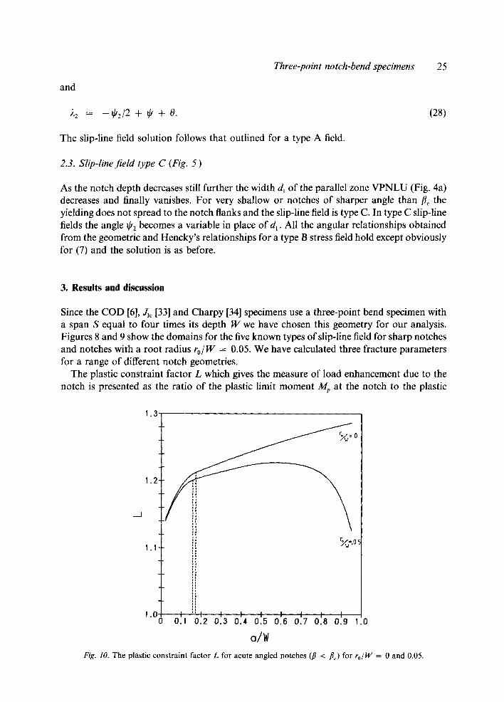
Since the COD [6], ,/zc [33] and Charpy [34] specimens use a three-point bend specimen with a span S equal to four times its depth W we have chosen this geometry for our analysis. Figures 8 and 9 show the domains for the five known types of slip-line field for sharp notches and notches with a root radius to~ W = 0.05. We have calculated three fracture parameters for a range of different notch geometries.

The plastic constraint factor L which gives the measure of load enhancement due to the notch is presented as the ratio of the plastic limit moment Mp at the notch to the plastic

..__1

1.3

1.2

1.1

1.0 0

~w =0

11 i! ii

I " 1 I I I I I I I 0 .1 0 . 2 0 . 3 0 . 4 0 . 5 0 . 6 0 . 7 0 . 8 0 . 9 1 .0

a/W Fig. 10. The plastic constraint factor L for acute angled notches (fl < #,) for ro/W = 0 and 0.05.


Table 1. Fracture parameters for sharp notches where yielding does not spread to the notch flanks (3 < 3c)

r o / W = O ~ < 3c

a /W 3c (°) L % / k r e

0.05 63.75 1.164 1.916 0.5131 0.1 50.78 1.192 2.369 0.5020 0.15 38.83 1.208 2.786 0.4731 0.172 33.44 1.212 2.974 0.4557 0.2 32.54 1.215 3.006 0.4547 0.3 29.31 1.227 3.118 0.4510 0.4 26.03 1.238 3.233 0.4472 0.5 22.71 1.249 3.349 0.4434 0.6 19.36 1.258 3.466 0.4395 0.7 15.98 1.267 3.584 0.4355 0.8 12.58 1.275 3.702 0.4316 0.9 9.19 1.283 3.821 0.4276

Table 2. Fracture parameters for acute angled notches of finite root radius where yielding does not spread to the notch flanks (3 < /~c)

a/W ro/W 3c (°) L a,,/k rp

0.05

0.5

0 63.75 1.164 1.916 0.5131 0.01 64.04 1.163 1.906 0.5240 0.02 64.32 1.163 1.897 0.5349 0.03 64.58 1.162 1.887 0.5457 0.04 64.84 1.161 1.878 0.5566 0.05 65.09 1.161 1.869 0.5674

0 22.71 1.249 3.349 0.4434 0.01 25.98 1.243 3.234 0.4466 0.02 28.83 1.238 3.135 0.4496 0.03 31.35 1.234 3.047 0.4524 0.04 33.60 1.230 2.969 0.4547 0.05 35.63 1.225 2.898 0.4573

moment for pure bending in a beam of equivalent depth (W - a). That is

L = 2Mp (29) k B W 2 ( 1 - a / W ) 2'

where k is the shear yield strength. The constraint factors for notches where yielding does not spread to the straight flanks of the notch (i.e.,/3 < /3c) are shown in Fig. 10 and in Tables 1 and 2. Table 3 gives the constraint factors for large angled notches (/3 > /3c)-

The slip-line field at the notch has been extended into the rigid region to R, following Green [2], and the maximum hydrostatic stress % is presented as a fraction of the shear yield strength k. The maximum hydrostatic stress thus depends on the angle $2 and is given by

a,,,/k = 1 + 202. (30)

The hydrostatic stress for acute angled cracks is shown in Fig. 11 and given in Tables 1 and 2. The values for large angles are given in Table 3.


Table 3. Fracture parameters for large angled notches where yielding spreads to the notch flanks (fl < fl,)

atW = 0.5

30 1.248 3.094 0.4435 45 1.246 2.571 0.4450 60 1.232 2.047 0.4505

0.025 45 1.224 2.571 0.4516 60 1.209 2.047 0.4558

0.05 45 1.210 2.571 0.4574 60 1.189 2.047 0.4605

The crack tip opening displacement ~ is extremely useful as a measure of the toughness of ductile metals. In the standard COD test [6] the plastic component of the crack tip opening displacement 6p can be determined from the plastic component Vp of the displacement measured at the crack mouth through (1). If yielding does not spread to the flanks the same equation can be used to calculate 8p provided the crack mouth opening is made with a clip gauge that is attached to the rigid region of the specimen KGEQV or either side of the notch [23]. However, some attention must be paid to the definition of crack tip opening displacement if the notch is not sharp and has a finite root radius. We have chosen to define the crack tip opening displacement at a notch with a finite root radius as the opening at the point where the root radius blends with the straight flanks of the notch. This definition is similar to that used by Robinson and Tetelman in their experimental work [35]. The rotation constant for sharp acute angled notches is shown in Fig. 12. The values are also tabulated

4.0-

3.0

2.0.

1.0

0 0

I: i: !.

i' ~5

i' I ;I I I I I I I I 0.1 0.2 0.3 0.4 0.5 0.6 0.7 O.B 0.9

o/w .0

Fig. 11. The hydrostatic stress o~/k for acute angled notches (fl < tic) for ro/W = 0 and 0.05.

28 S.X. Wu, B. Cotterell and Y. I4". Mai

0.6"

0.5-

0.4

0.3

0.2 0

t ' 1 I I I I I I I 0.1 0.2 0.3 0.4 0.5 0.6 0.7 0.8 0.9 1.0

a/W Fig. 12. The rotation constant rp for sharp angled notches (fl < /~c, ro/W = 0).

in Tables 1-3. For the special case of a sharp crack that is the most usual fracture specimen we have obtained a simple expression for shallow crack to supplement our previous expression for deep cracks [7]. These two expression, which are accurate to within 0.5 percent, are

0.463 - 0.04 a/W for a/W > 0.172

rp = 0.5 + 0.42 a/W - 4(a/W) 2 for a/W < 0~172. (31)

For shallow cracks r e reaches a maximum of 0.513 at about a/W = 0.05.

Acknowledgements

We wish to thank the Australian Research Grants Scheme and the Australian Welding Research Association for the financial support of this work. One of us (S.-X. Wu) is supported by a Sydney University Postgraduate Research Scholarship.

References

1. A.P. Green and B.B. Hundy, Journal of the Mechanics and Physics of Solids 4 (1956) 128-44. 2. A.P. Green, Journal of the Mechanics and Physics of Solids 4 (1956) 259-68. 3. J.M. Alexander and T.J. Komoly, Journal of the Mechanics and Physics of Solids 10 (1962) 265-75. 4. J.F. Knott, Journal of the Iron and Steel Institute 204 (1966) 104-11.

Three-poin t no tch-bend spec imens 29

5. D.J.F. Ewing, Journal of the Mechanics and Physics of Solids 16 (1968) 205-13. 6. British Standards, Methods for crack opening displacement (COD) testing, BS 5762 (1979). 7. G. Matsoukas, B. Cotterell and Y.-W. Mai, International Journal of Fracture 26 (1984) R49-R53. 8. S.-X. Wu, Engineering Fracture Mechanics 18 (1983) 83-95. 9. I.-H. Lin, T.L. Anderson, R. deWit and M.G. Dawes, International Journal of Fracture 20 (1982) R3-R7.

10. G.A. Clarke, W.R. Andrews, J.A. Begley, J.K. Donald, G.T. Embley, J.D. Landes, D.E. McCabe and J.H. Underwood, Journal of Testing and Evaluation 7 (1979) 49-56.

11. British Standard, Guidance on some methods for the derivation of acceptance levels for defects infusion welded joints, PD 6493 (1980).

12. M.S. Kamath, The COD design curve." an assessment of validity using wide plate tests, Welding Institute Report 71/1978/E.

13. C.G. Chipperfield, Proceedings, Specialists Meeting in Elasto-Plastic Fracture Mechanics, OECD Nuclear Energy Agency Daresbury, Vol. 2, Paper 15.

14. B. Cotterell, Q.-F. Li, D.-Z. Zhang and Y.-W. Mai, Engineering Fracture Mechanics 24 (1986) 837 842. 15. G. Matsoukas, B. Cotterell and Y.-W. Mai, Engineering Fracture Mechanics 23 (1986) 661-665. 16. H.E. Thompson and J.F. Knott, Fracture Control of Engineering Structures. ECF 6 (1986). 17. P.W. Bridgman, Large Plastic Flow and Fracture, McGraw Hill, New York (1952). 18. K.E. Puttick, Philosophical Magazine, Ser. A, 4 (1959) 964-69. 1'9. F.A. McClintock, Journal of Applied Mechanics 35 (1968) 363. 20. G. Matsoukas, B. Cotterell and Y.-W. Mai, Engineering Fracture Mechanics 23 (1986) 661-65. 21. A.P. Green, Quarterly Journal of Mechanics and Applied Mathematics 6 (1953) 223 39. 22. A. Shindo and Y. Tomita, Bulletin of the Japan Society for Mechanical Engineering 15 (1972) 11-20. 23. G. Matsoukas, B. Cotterell and Y.-W. Mai, Journal of the Mechanics and Physics of Solids 34 (1986) 499-510. 24. D.J.F. Ewing, Doctoral Thesis, Cambridge University (1968). 25. D.J.F. Ewing, Journal of the Mechanics and Physics of Solids 15 (1967) 105-I 14. 26. I.F. Collins, Proceeding of the Royal Society, A303 (1968) 307. 27. P. Dewhurst and I.F. Collins, International Journal for Numerical Methods in Engineering 7 (1973) 357 378. 28. W. Johnson, R. Sowerby and R,D. Venter, Plane Strain Slip Line Fields for Metal Del'ormation Processes,

Pergamon Press, Oxford (1982). 29. S.-X. Wu, Y.-W. Mai and B. Cotterell, International Journal of Mechanical Sciences 29 (1987)557-564. 30. A. Shindo and Y. Tomita, Memoirs of the Faculty of Engineering, Tobe University, No. 20 (1974) 59 67. 31. J.F.W. Bishop, Journal of the Mechanics of Physics of Solids 2 (1953) 43-53. 32. NAG Fortran library routine document CO5MBF. 33. ASTM Standard test for Jr,. a measure of fracture toughness, E813-81. 34. British Standards, Methods for notched bar tests, The Charpy V-notch impact test on metals, BS 131: Part

2 (1972). 35. J.N. Robinson and A.S. Tetelman, International Journal of Fracture 11 (1975) 453 469.

R~sum6. On passe en revue les solutions d6crivant les champs de bandes de glissement dans des 6prouvettes de flexion sur trois appuis, dans les deux cas d'entailles peu profondes. On fournit'pour une large gamme de g6om~tries d'entaille les facteurs de retraint plastique, les contraintes hydrostatiques fi la racine de l'entaille et la constante de rotation pennettant de d~terminer le COD h l'extrbmit6 de la fissure. Ces valeurs peuvent &re utilis6es pour l'analyse de la rupture des 6prouvettes de mbtaux ~ faible r6sistance.

slip-line field solutions for three-point notch-bend specimens

Documents