slides prepared by john s. loucks st. edward’s university
DESCRIPTION
Slides Prepared by JOHN S. LOUCKS St. Edward’s University. .40. .30. .20. .10. 0 1 2 3 4. Chapter 5 Discrete Probability Distributions. Random Variables. Discrete Probability Distributions. Expected Value and Variance. Binomial Distribution. - PowerPoint PPT PresentationTRANSCRIPT
1 1 Slide
Slide
© 2006 Thomson/South-Western© 2006 Thomson/South-Western
Slides Prepared bySlides Prepared by
JOHN S. LOUCKSJOHN S. LOUCKSSt. Edward’s UniversitySt. Edward’s University
Slides Prepared bySlides Prepared by
JOHN S. LOUCKSJOHN S. LOUCKSSt. Edward’s UniversitySt. Edward’s University

2 2 Slide
Slide
© 2006 Thomson/South-Western© 2006 Thomson/South-Western
Chapter 5Chapter 5 Discrete Probability Distributions Discrete Probability Distributions
.10.10
.20.20
.30.30
.40.40
0 1 2 3 4 0 1 2 3 4
Random VariablesRandom Variables Discrete Probability DistributionsDiscrete Probability Distributions Expected Value and VarianceExpected Value and Variance Binomial DistributionBinomial Distribution Poisson DistributionPoisson Distribution Hypergeometric DistributionHypergeometric Distribution

3 3 Slide
Slide
© 2006 Thomson/South-Western© 2006 Thomson/South-Western
A A random variablerandom variable is a numerical description of the is a numerical description of the outcome of an experiment.outcome of an experiment. A A random variablerandom variable is a numerical description of the is a numerical description of the outcome of an experiment.outcome of an experiment.
Random VariablesRandom Variables
A A discrete random variablediscrete random variable may assume either a may assume either a finite number of values or an infinite sequence offinite number of values or an infinite sequence of values.values.
A A discrete random variablediscrete random variable may assume either a may assume either a finite number of values or an infinite sequence offinite number of values or an infinite sequence of values.values.
A A continuous random variablecontinuous random variable may assume any may assume any numerical value in an interval or collection ofnumerical value in an interval or collection of intervals.intervals.
A A continuous random variablecontinuous random variable may assume any may assume any numerical value in an interval or collection ofnumerical value in an interval or collection of intervals.intervals.
4 4 Slide
Slide
© 2006 Thomson/South-Western© 2006 Thomson/South-Western
Let Let xx = number of TVs sold at the store in one day, = number of TVs sold at the store in one day,
where where xx can take on 5 values (0, 1, 2, 3, 4) can take on 5 values (0, 1, 2, 3, 4)
Let Let xx = number of TVs sold at the store in one day, = number of TVs sold at the store in one day,
where where xx can take on 5 values (0, 1, 2, 3, 4) can take on 5 values (0, 1, 2, 3, 4)
Example: JSL AppliancesExample: JSL Appliances
Discrete random variable with a Discrete random variable with a finitefinite number number of values of values

5 5 Slide
Slide
© 2006 Thomson/South-Western© 2006 Thomson/South-Western
Let Let xx = number of customers arriving in one day, = number of customers arriving in one day,
where where xx can take on the values 0, 1, 2, . . . can take on the values 0, 1, 2, . . .
Let Let xx = number of customers arriving in one day, = number of customers arriving in one day,
where where xx can take on the values 0, 1, 2, . . . can take on the values 0, 1, 2, . . .
Example: JSL AppliancesExample: JSL Appliances
Discrete random variable with an Discrete random variable with an infiniteinfinite sequence of valuessequence of values
We can count the customers arriving, but there is noWe can count the customers arriving, but there is nofinite upper limit on the number that might arrive.finite upper limit on the number that might arrive.

6 6 Slide
Slide
© 2006 Thomson/South-Western© 2006 Thomson/South-Western
Random VariablesRandom Variables
QuestionQuestion Random Variable Random Variable xx TypeType
FamilyFamilysizesize
xx = Number of dependents = Number of dependents reported on tax returnreported on tax return
DiscreteDiscrete
Distance fromDistance fromhome to storehome to store
xx = Distance in miles from = Distance in miles from home to the store sitehome to the store site
ContinuousContinuous
Own dogOwn dogor cator cat
xx = 1 if own no pet; = 1 if own no pet; = 2 if own dog(s) only; = 2 if own dog(s) only; = 3 if own cat(s) only; = 3 if own cat(s) only; = 4 if own dog(s) and cat(s)= 4 if own dog(s) and cat(s)
DiscreteDiscrete

7 7 Slide
Slide
© 2006 Thomson/South-Western© 2006 Thomson/South-Western
The The probability distributionprobability distribution for a random variable for a random variable describes how probabilities are distributed overdescribes how probabilities are distributed over the values of the random variable.the values of the random variable.
The The probability distributionprobability distribution for a random variable for a random variable describes how probabilities are distributed overdescribes how probabilities are distributed over the values of the random variable.the values of the random variable.
We can describe a discrete probability distributionWe can describe a discrete probability distribution with a table, graph, or equation.with a table, graph, or equation. We can describe a discrete probability distributionWe can describe a discrete probability distribution with a table, graph, or equation.with a table, graph, or equation.
Discrete Probability DistributionsDiscrete Probability Distributions
8 8 Slide
Slide
© 2006 Thomson/South-Western© 2006 Thomson/South-Western
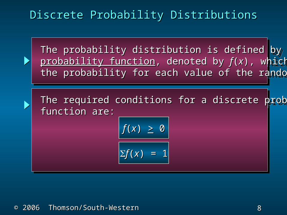
The probability distribution is defined by aThe probability distribution is defined by a probability functionprobability function, denoted by , denoted by ff((xx), which provides), which provides the probability for each value of the random variable.the probability for each value of the random variable.
The probability distribution is defined by aThe probability distribution is defined by a probability functionprobability function, denoted by , denoted by ff((xx), which provides), which provides the probability for each value of the random variable.the probability for each value of the random variable.
The required conditions for a discrete probabilityThe required conditions for a discrete probability function are:function are: The required conditions for a discrete probabilityThe required conditions for a discrete probability function are:function are:
Discrete Probability DistributionsDiscrete Probability Distributions
ff((xx) ) >> 0 0ff((xx) ) >> 0 0
ff((xx) = 1) = 1ff((xx) = 1) = 1

9 9 Slide
Slide
© 2006 Thomson/South-Western© 2006 Thomson/South-Western
a tabular representation of the probabilitya tabular representation of the probability distribution for TV sales was developed.distribution for TV sales was developed.
Using past data on TV sales, …Using past data on TV sales, …
NumberNumber Units SoldUnits Sold of Daysof Days
00 80 80 11 50 50 22 40 40 33 10 10 44 20 20
200200
xx ff((xx)) 00 .40 .40 11 .25 .25 22 .20 .20 33 .05 .05 44 .10 .10
1.001.00
80/20080/200
Discrete Probability DistributionsDiscrete Probability Distributions

10 10 Slide
Slide
© 2006 Thomson/South-Western© 2006 Thomson/South-Western
.10.10
.20.20
.30.30
.40.40
.50.50
0 1 2 3 40 1 2 3 4Values of Random Variable Values of Random Variable xx (TV sales) (TV sales)Values of Random Variable Values of Random Variable xx (TV sales) (TV sales)
Pro
babili
tyPro
babili
tyPro
babili
tyPro
babili
ty
Discrete Probability DistributionsDiscrete Probability Distributions
Graphical Representation of Probability DistributionGraphical Representation of Probability Distribution

11 11 Slide
Slide
© 2006 Thomson/South-Western© 2006 Thomson/South-Western
Discrete Uniform Probability DistributionDiscrete Uniform Probability Distribution
The The discrete uniform probability distributiondiscrete uniform probability distribution is the is the simplest example of a discrete probabilitysimplest example of a discrete probability distribution given by a formula.distribution given by a formula.
The The discrete uniform probability distributiondiscrete uniform probability distribution is the is the simplest example of a discrete probabilitysimplest example of a discrete probability distribution given by a formula.distribution given by a formula.
The The discrete uniform probability functiondiscrete uniform probability function is is The The discrete uniform probability functiondiscrete uniform probability function is is
ff((xx) = 1/) = 1/nnff((xx) = 1/) = 1/nn
where:where:nn = the number of values the random = the number of values the random variable may assumevariable may assume
the values of the values of thethe
random random variablevariable
are equally are equally likelylikely

12 12 Slide
Slide
© 2006 Thomson/South-Western© 2006 Thomson/South-Western
Expected Value and VarianceExpected Value and Variance
The The expected valueexpected value, or mean, of a random variable, or mean, of a random variable is a measure of its central location.is a measure of its central location. The The expected valueexpected value, or mean, of a random variable, or mean, of a random variable is a measure of its central location.is a measure of its central location.
The The variancevariance summarizes the variability in the summarizes the variability in the values of a random variable.values of a random variable. The The variancevariance summarizes the variability in the summarizes the variability in the values of a random variable.values of a random variable.
The The standard deviationstandard deviation, , , is defined as the positive, is defined as the positive square root of the variance.square root of the variance. The The standard deviationstandard deviation, , , is defined as the positive, is defined as the positive square root of the variance.square root of the variance.
Var(Var(xx) = ) = 22 = = ((xx - - ))22ff((xx))Var(Var(xx) = ) = 22 = = ((xx - - ))22ff((xx))
EE((xx) = ) = = = xfxf((xx))EE((xx) = ) = = = xfxf((xx))

13 13 Slide
Slide
© 2006 Thomson/South-Western© 2006 Thomson/South-Western
Expected ValueExpected Value
expected number expected number of TVs sold in a dayof TVs sold in a day
xx ff((xx)) xfxf((xx))
00 .40 .40 .00 .00
11 .25 .25 .25 .25
22 .20 .20 .40 .40
33 .05 .05 .15 .15
44 .10 .10 .40.40
EE((xx) = 1.20) = 1.20
Expected Value and VarianceExpected Value and Variance

14 14 Slide
Slide
© 2006 Thomson/South-Western© 2006 Thomson/South-Western
Variance and Standard DeviationVariance and Standard Deviation
00
11
22
33
44
-1.2-1.2
-0.2-0.2
0.80.8
1.81.8
2.82.8
1.441.44
0.040.04
0.640.64
3.243.24
7.847.84
.40.40
.25.25
.20.20
.05.05
.10.10
.576.576
.010.010
.128.128
.162.162
.784.784
x - x - ((x - x - ))22 ff((xx)) ((xx - - ))22ff((xx))
Variance of daily sales = Variance of daily sales = 22 = 1.660 = 1.660
xx
TVsTVssquaresquare
dd
Standard deviation of daily sales = 1.2884 TVsStandard deviation of daily sales = 1.2884 TVs
Expected Value and VarianceExpected Value and Variance
15 15 Slide
Slide
© 2006 Thomson/South-Western© 2006 Thomson/South-Western
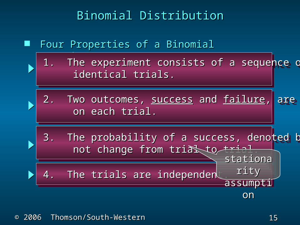
Binomial DistributionBinomial Distribution
Four Properties of a Binomial ExperimentFour Properties of a Binomial Experiment
3. The probability of a success, denoted by 3. The probability of a success, denoted by pp, does, does not change from trial to trial.not change from trial to trial.3. The probability of a success, denoted by 3. The probability of a success, denoted by pp, does, does not change from trial to trial.not change from trial to trial.
4. The trials are independent.4. The trials are independent.4. The trials are independent.4. The trials are independent.
2. Two outcomes, 2. Two outcomes, successsuccess and and failurefailure, are possible, are possible on each trial.on each trial.2. Two outcomes, 2. Two outcomes, successsuccess and and failurefailure, are possible, are possible on each trial.on each trial.
1. The experiment consists of a sequence of 1. The experiment consists of a sequence of nn identical trials.identical trials.1. The experiment consists of a sequence of 1. The experiment consists of a sequence of nn identical trials.identical trials.
stationaritstationarityy
assumptioassumptionn

16 16 Slide
Slide
© 2006 Thomson/South-Western© 2006 Thomson/South-Western
Binomial DistributionBinomial Distribution
Our interest is in the Our interest is in the number of successesnumber of successes occurring in the occurring in the nn trials. trials. Our interest is in the Our interest is in the number of successesnumber of successes occurring in the occurring in the nn trials. trials.
We let We let xx denote the number of successes denote the number of successes occurring in the occurring in the nn trials. trials. We let We let xx denote the number of successes denote the number of successes occurring in the occurring in the nn trials. trials.
17 17 Slide
Slide
© 2006 Thomson/South-Western© 2006 Thomson/South-Western
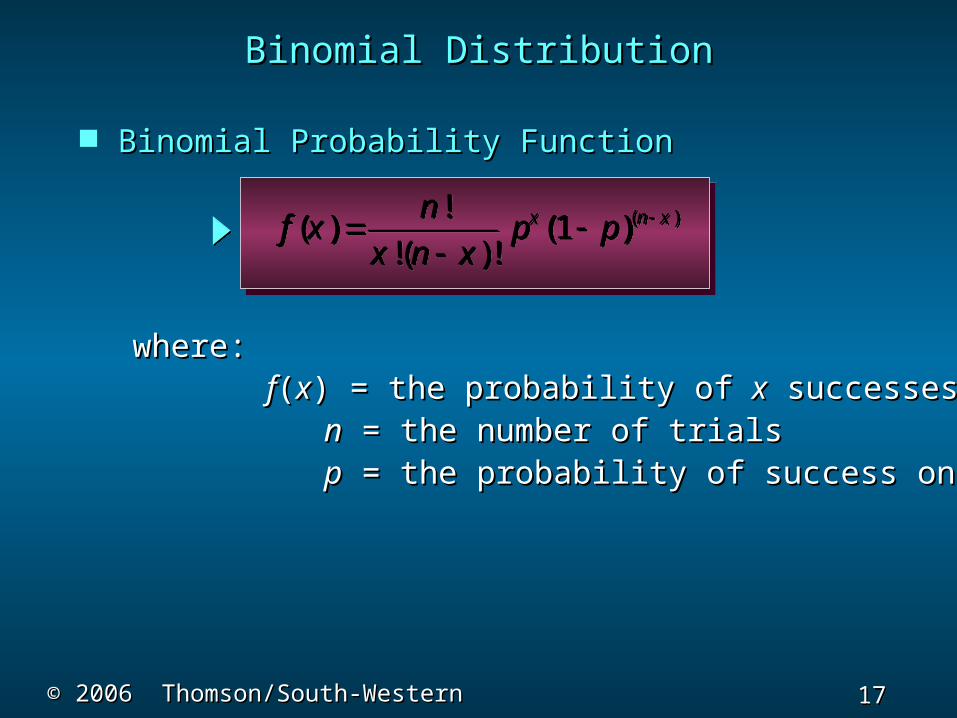
where:where: ff((xx) = the probability of ) = the probability of xx successes in successes in nn trials trials nn = the number of trials = the number of trials pp = the probability of success on any one trial = the probability of success on any one trial
( )!( ) (1 )
!( )!x n xn
f x p px n x
( )!( ) (1 )
!( )!x n xn
f x p px n x
Binomial DistributionBinomial Distribution
Binomial Probability FunctionBinomial Probability Function

18 18 Slide
Slide
© 2006 Thomson/South-Western© 2006 Thomson/South-Western
( )!( ) (1 )
!( )!x n xn
f x p px n x
( )!( ) (1 )
!( )!x n xn
f x p px n x
Binomial DistributionBinomial Distribution
!!( )!
nx n x
!!( )!
nx n x
( )(1 )x n xp p ( )(1 )x n xp p
Binomial Probability FunctionBinomial Probability Function
Probability of a particularProbability of a particular sequence of trial outcomessequence of trial outcomes with x successes in with x successes in nn trials trials
Probability of a particularProbability of a particular sequence of trial outcomessequence of trial outcomes with x successes in with x successes in nn trials trials
Number of experimentalNumber of experimental outcomes providing exactlyoutcomes providing exactly
xx successes in successes in nn trials trials
Number of experimentalNumber of experimental outcomes providing exactlyoutcomes providing exactly
xx successes in successes in nn trials trials
19 19 Slide
Slide
© 2006 Thomson/South-Western© 2006 Thomson/South-Western
Binomial DistributionBinomial Distribution
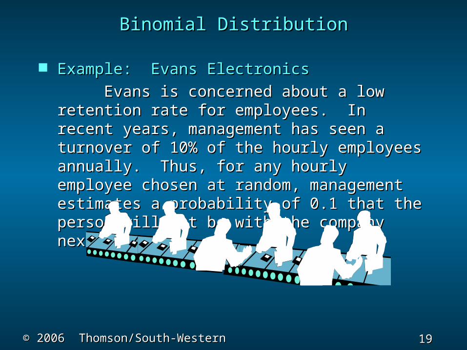
Example: Evans ElectronicsExample: Evans Electronics
Evans is concerned about a low retention Evans is concerned about a low retention rate for employees. In recent years, rate for employees. In recent years, management has seen a turnover of 10% of management has seen a turnover of 10% of the hourly employees annually. Thus, for any the hourly employees annually. Thus, for any hourly employee chosen at random, hourly employee chosen at random, management estimates a probability of 0.1 management estimates a probability of 0.1 that the person will not be with the company that the person will not be with the company next year.next year.

20 20 Slide
Slide
© 2006 Thomson/South-Western© 2006 Thomson/South-Western
Binomial DistributionBinomial Distribution
Using the Binomial Probability FunctionUsing the Binomial Probability Function
Choosing 3 hourly employees at random, Choosing 3 hourly employees at random, what is the probability that 1 of them will leave what is the probability that 1 of them will leave the company this year?the company this year?
f xn
x n xp px n x( )
!!( )!
( )( )
1f xn
x n xp px n x( )
!!( )!
( )( )
1
1 23!(1) (0.1) (0.9) 3(.1)(.81) .243
1!(3 1)!f
1 23!
(1) (0.1) (0.9) 3(.1)(.81) .2431!(3 1)!
f
LetLet: p: p = .10, = .10, nn = 3, = 3, xx = 1 = 1

21 21 Slide
Slide
© 2006 Thomson/South-Western© 2006 Thomson/South-Western
Tree DiagramTree Diagram
Binomial DistributionBinomial Distribution
1st Worker 1st Worker 2nd Worker2nd Worker 3rd Worker3rd Worker xx Prob.Prob.
Leaves (.1)Leaves (.1)
Stays (.9)Stays (.9)
33
22
00
22
22
Leaves (.1)Leaves (.1)
Leaves (.1)Leaves (.1)
S (.9)S (.9)
Stays (.9)Stays (.9)
Stays (.9)Stays (.9)
S (.9)S (.9)
S (.9)S (.9)
S (.9)S (.9)
L (.1)L (.1)
L (.1)L (.1)
L (.1)L (.1)
L (.1)L (.1) .0010.0010
.0090.0090
.0090.0090
.7290.7290
.0090.0090
11
11
.0810.0810
.0810.0810
.0810.0810
1111

22 22 Slide
Slide
© 2006 Thomson/South-Western© 2006 Thomson/South-Western
Using Tables of Binomial ProbabilitiesUsing Tables of Binomial Probabilities
n x .05 .10 .15 .20 .25 .30 .35 .40 .45 .50
3 0 .8574 .7290 .6141 .5120 .4219 .3430 .2746 .2160 .1664 .12501 .1354 .2430 .3251 .3840 .4219 .4410 .4436 .4320 .4084 .37502 .0071 .0270 .0574 .0960 .1406 .1890 .2389 .2880 .3341 .37503 .0001 .0010 .0034 .0080 .0156 .0270 .0429 .0640 .0911 .1250
pn x .05 .10 .15 .20 .25 .30 .35 .40 .45 .50
3 0 .8574 .7290 .6141 .5120 .4219 .3430 .2746 .2160 .1664 .12501 .1354 .2430 .3251 .3840 .4219 .4410 .4436 .4320 .4084 .37502 .0071 .0270 .0574 .0960 .1406 .1890 .2389 .2880 .3341 .37503 .0001 .0010 .0034 .0080 .0156 .0270 .0429 .0640 .0911 .1250
p
Binomial DistributionBinomial Distribution
23 23 Slide
Slide
© 2006 Thomson/South-Western© 2006 Thomson/South-Western
Binomial DistributionBinomial Distribution
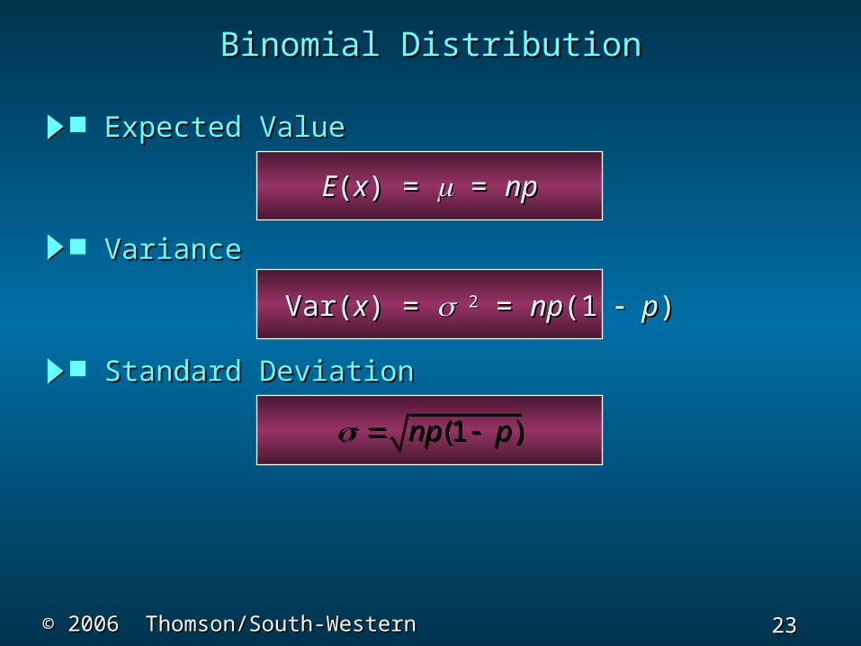
(1 )np p (1 )np p
EE((xx) = ) = = = npnp
Var(Var(xx) = ) = 22 = = npnp(1 (1 pp))
Expected ValueExpected Value
VarianceVariance
Standard DeviationStandard Deviation

24 24 Slide
Slide
© 2006 Thomson/South-Western© 2006 Thomson/South-Western
Binomial DistributionBinomial Distribution
3(.1)(.9) .52 employees 3(.1)(.9) .52 employees
EE((xx) = ) = = 3(.1) = .3 employees out of 3 = 3(.1) = .3 employees out of 3
Var(Var(xx) = ) = 22 = 3(.1)(.9) = .27 = 3(.1)(.9) = .27
Expected ValueExpected Value
VarianceVariance
Standard DeviationStandard Deviation

25 25 Slide
Slide
© 2006 Thomson/South-Western© 2006 Thomson/South-Western
A Poisson distributed random variable is oftenA Poisson distributed random variable is often useful in estimating the number of occurrencesuseful in estimating the number of occurrences over a over a specified interval of time or spacespecified interval of time or space
A Poisson distributed random variable is oftenA Poisson distributed random variable is often useful in estimating the number of occurrencesuseful in estimating the number of occurrences over a over a specified interval of time or spacespecified interval of time or space
It is a discrete random variable that may assumeIt is a discrete random variable that may assume an an infinite sequence of valuesinfinite sequence of values (x = 0, 1, 2, . . . ). (x = 0, 1, 2, . . . ). It is a discrete random variable that may assumeIt is a discrete random variable that may assume an an infinite sequence of valuesinfinite sequence of values (x = 0, 1, 2, . . . ). (x = 0, 1, 2, . . . ).
Poisson DistributionPoisson Distribution

26 26 Slide
Slide
© 2006 Thomson/South-Western© 2006 Thomson/South-Western
Examples of a Poisson distributed random variable:Examples of a Poisson distributed random variable: Examples of a Poisson distributed random variable:Examples of a Poisson distributed random variable:
the number of knotholes in 14 linear feet ofthe number of knotholes in 14 linear feet of pine boardpine board the number of knotholes in 14 linear feet ofthe number of knotholes in 14 linear feet of pine boardpine board
the number of vehicles arriving at athe number of vehicles arriving at a toll booth in one hourtoll booth in one hour the number of vehicles arriving at athe number of vehicles arriving at a toll booth in one hourtoll booth in one hour
Poisson DistributionPoisson Distribution
27 27 Slide
Slide
© 2006 Thomson/South-Western© 2006 Thomson/South-Western
Poisson DistributionPoisson Distribution
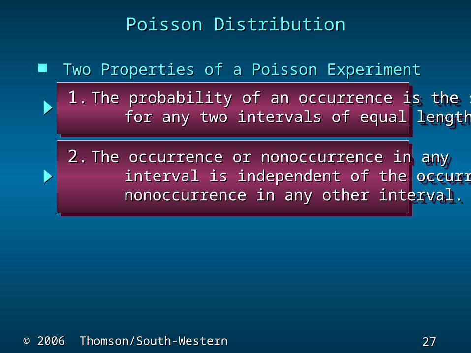
Two Properties of a Poisson ExperimentTwo Properties of a Poisson Experiment
2.2. The occurrence or nonoccurrence in anyThe occurrence or nonoccurrence in any interval is independent of the occurrence orinterval is independent of the occurrence or nonoccurrence in any other interval.nonoccurrence in any other interval.
2.2. The occurrence or nonoccurrence in anyThe occurrence or nonoccurrence in any interval is independent of the occurrence orinterval is independent of the occurrence or nonoccurrence in any other interval.nonoccurrence in any other interval.
1.1. The probability of an occurrence is the sameThe probability of an occurrence is the same for any two intervals of equal length.for any two intervals of equal length.1.1. The probability of an occurrence is the sameThe probability of an occurrence is the same for any two intervals of equal length.for any two intervals of equal length.

28 28 Slide
Slide
© 2006 Thomson/South-Western© 2006 Thomson/South-Western
Poisson Probability FunctionPoisson Probability Function
Poisson DistributionPoisson Distribution
f xe
x
x( )
!
f x
e
x
x( )
!
where:where:
f(x) f(x) = probability of = probability of xx occurrences in an interval occurrences in an interval
= mean number of occurrences in an interval= mean number of occurrences in an interval
ee = 2.71828 = 2.71828
29 29 Slide
Slide
© 2006 Thomson/South-Western© 2006 Thomson/South-Western
Poisson DistributionPoisson Distribution
MERCYMERCY
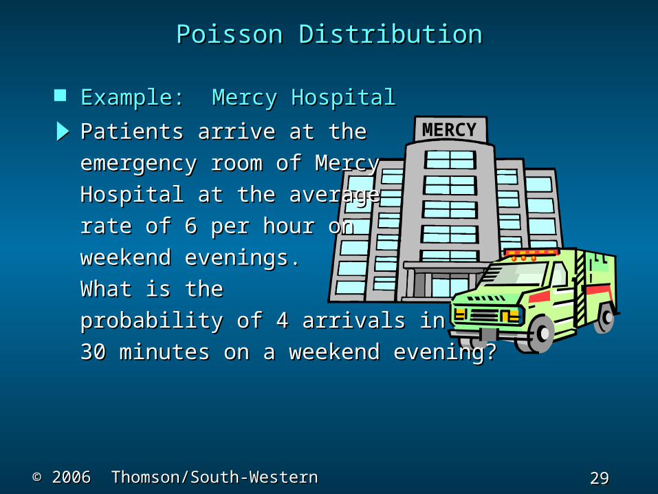
Example: Mercy HospitalExample: Mercy Hospital
Patients arrive at the Patients arrive at the
emergency room of Mercyemergency room of Mercy
Hospital at the averageHospital at the average
rate of 6 per hour onrate of 6 per hour on
weekend evenings. weekend evenings.
What is theWhat is the
probability of 4 arrivals inprobability of 4 arrivals in
30 minutes on a weekend evening?30 minutes on a weekend evening?

30 30 Slide
Slide
© 2006 Thomson/South-Western© 2006 Thomson/South-Western
Poisson DistributionPoisson Distribution
Using the Poisson Probability FunctionUsing the Poisson Probability Function
4 33 (2.71828)(4) .1680
4!f
4 33 (2.71828)
(4) .16804!
f
MERCYMERCY
= 6/hour = 3/half-hour, = 6/hour = 3/half-hour, xx = 4 = 4

31 31 Slide
Slide
© 2006 Thomson/South-Western© 2006 Thomson/South-Western
Poisson DistributionPoisson Distribution
Using Poisson Probability TablesUsing Poisson Probability Tables
x 2.1 2.2 2.3 2.4 2.5 2.6 2.7 2.8 2.9 3.00 .1225 .1108 .1003 .0907 .0821 .0743 .0672 .0608 .0550 .04981 .2572 .2438 .2306 .2177 .2052 .1931 .1815 .1703 .1596 .14942 .2700 .2681 .2652 .2613 .2565 .2510 .2450 .2384 .2314 .22403 .1890 .1966 .2033 .2090 .2138 .2176 .2205 .2225 .2237 .22404 .0992 .1082 .1169 .1254 .1336 .1414 .1488 .1557 .1622 .16805 .0417 .0476 .0538 .0602 ..0668 .0735 .0804 .0872 .0940 .10086 .0146 .0174 .0206 .0241 .0278 .0319 .0362 .0407 .0455 .05047 .0044 .0055 .0068 .0083 .0099 .0118 .0139 .0163 .0188 .02168 .0011 .0015 .0019 .0025 .0031 .0038 .0047 .0057 .0068 .0081
x 2.1 2.2 2.3 2.4 2.5 2.6 2.7 2.8 2.9 3.00 .1225 .1108 .1003 .0907 .0821 .0743 .0672 .0608 .0550 .04981 .2572 .2438 .2306 .2177 .2052 .1931 .1815 .1703 .1596 .14942 .2700 .2681 .2652 .2613 .2565 .2510 .2450 .2384 .2314 .22403 .1890 .1966 .2033 .2090 .2138 .2176 .2205 .2225 .2237 .22404 .0992 .1082 .1169 .1254 .1336 .1414 .1488 .1557 .1622 .16805 .0417 .0476 .0538 .0602 ..0668 .0735 .0804 .0872 .0940 .10086 .0146 .0174 .0206 .0241 .0278 .0319 .0362 .0407 .0455 .05047 .0044 .0055 .0068 .0083 .0099 .0118 .0139 .0163 .0188 .02168 .0011 .0015 .0019 .0025 .0031 .0038 .0047 .0057 .0068 .0081
MERCYMERCY

32 32 Slide
Slide
© 2006 Thomson/South-Western© 2006 Thomson/South-Western
Poisson Distribution of ArrivalsPoisson Distribution of Arrivals
Poisson DistributionPoisson DistributionMERCYMERCY
Poisson Probabilities
0.00
0.05
0.10
0.15
0.20
0.25
0 1 2 3 4 5 6 7 8 9 10
Number of Arrivals in 30 Minutes
Pro
bab
ilit
y
actually, actually, the the
sequencesequencecontinues:continues:11, 12, …11, 12, …
33 33 Slide
Slide
© 2006 Thomson/South-Western© 2006 Thomson/South-Western
Poisson DistributionPoisson Distribution
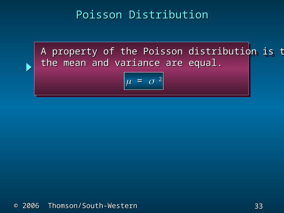
A property of the Poisson distribution is thatA property of the Poisson distribution is thatthe mean and variance are equal.the mean and variance are equal.
A property of the Poisson distribution is thatA property of the Poisson distribution is thatthe mean and variance are equal.the mean and variance are equal.
= = 22

34 34 Slide
Slide
© 2006 Thomson/South-Western© 2006 Thomson/South-Western
Poisson DistributionPoisson DistributionMERCYMERCY
Variance for Number of ArrivalsVariance for Number of Arrivals
During 30-Minute PeriodsDuring 30-Minute Periods
= = 22 = 3 = 3 = = 22 = 3 = 3
35 35 Slide
Slide
© 2006 Thomson/South-Western© 2006 Thomson/South-Western
Hypergeometric DistributionHypergeometric Distribution
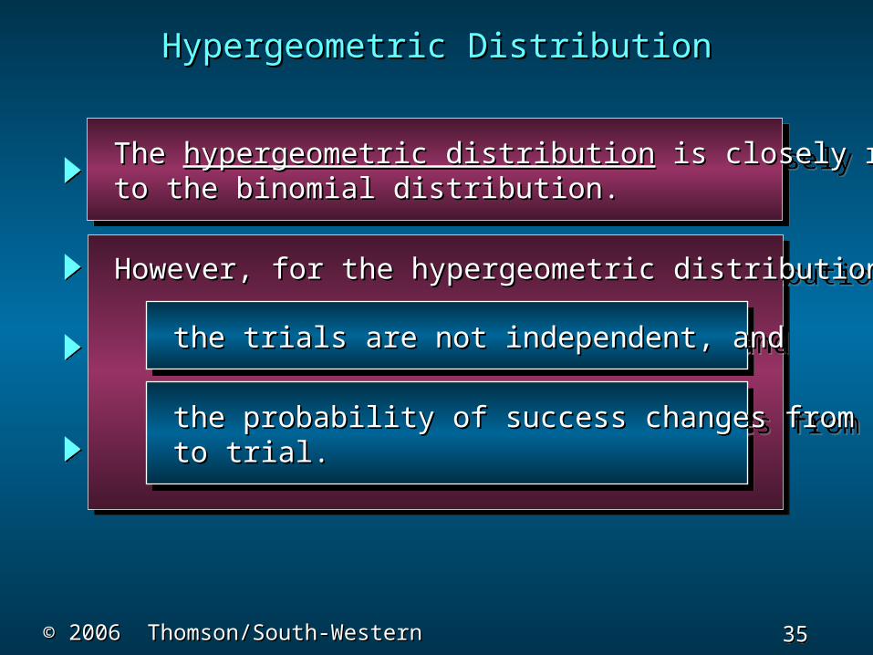
The The hypergeometric distributionhypergeometric distribution is closely related is closely related to the binomial distribution. to the binomial distribution. The The hypergeometric distributionhypergeometric distribution is closely related is closely related to the binomial distribution. to the binomial distribution.
However, for the hypergeometric distribution:However, for the hypergeometric distribution: However, for the hypergeometric distribution:However, for the hypergeometric distribution:
the trials are not independent, andthe trials are not independent, and the trials are not independent, andthe trials are not independent, and
the probability of success changes from trialthe probability of success changes from trial to trial. to trial. the probability of success changes from trialthe probability of success changes from trial to trial. to trial.
36 36 Slide
Slide
© 2006 Thomson/South-Western© 2006 Thomson/South-Western
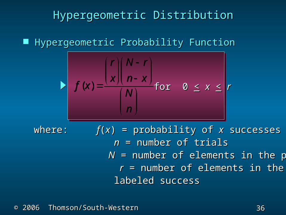
Hypergeometric Probability FunctionHypergeometric Probability Function
Hypergeometric DistributionHypergeometric Distribution
n
N
xn
rN
x
r
xf )(
n
N
xn
rN
x
r
xf )( for 0 for 0 << xx << rr
where: where: ff((xx) = probability of ) = probability of xx successes in successes in nn trials trials nn = number of trials = number of trials NN = number of elements in the population = number of elements in the population rr = number of elements in the population = number of elements in the population
labeled successlabeled success

37 37 Slide
Slide
© 2006 Thomson/South-Western© 2006 Thomson/South-Western
Hypergeometric Probability FunctionHypergeometric Probability Function
Hypergeometric DistributionHypergeometric Distribution
( )
r N r
x n xf x
N
n
( )
r N r
x n xf x
N
n
for 0 for 0 << xx << rr
number of waysnumber of waysnn – – x x failures can be selectedfailures can be selectedfrom a total of from a total of NN – – rr failures failures
in the populationin the populationnumber of waysnumber of ways
xx successes can be selected successes can be selectedfrom a total of from a total of rr successes successes
in the populationin the populationnumber of waysnumber of ways
a sample of size a sample of size n n can be selectedcan be selectedfrom a population of size from a population of size NN
38 38 Slide
Slide
© 2006 Thomson/South-Western© 2006 Thomson/South-Western
Hypergeometric DistributionHypergeometric Distribution
Example: NevereadyExample: NevereadyBob Neveready has removed twoBob Neveready has removed two
dead batteries from a flashlight anddead batteries from a flashlight andinadvertently mingled them withinadvertently mingled them withthe two good batteries he intendedthe two good batteries he intendedas replacements. as replacements. The four batteries look The four batteries look identical.identical.
Bob now randomly selects two of the Bob now randomly selects two of the four batteries. What is the probability he four batteries. What is the probability he selects the two good batteries?selects the two good batteries?
ZAPZAP ZA
PZ
AP
ZAP ZAPZAPZAP

39 39 Slide
Slide
© 2006 Thomson/South-Western© 2006 Thomson/South-Western
Hypergeometric DistributionHypergeometric Distribution
Using the Hypergeometric FunctionUsing the Hypergeometric Function
2 2 2! 2!
2 0 2!0! 0!2! 1( ) .167
4 4! 62 2!2!
r N r
x n xf x
N
n
2 2 2! 2!
2 0 2!0! 0!2! 1( ) .167
4 4! 62 2!2!
r N r
x n xf x
N
n
where:where: xx = 2 = number of = 2 = number of goodgood batteries selected batteries selected
nn = 2 = number of batteries selected = 2 = number of batteries selected NN = 4 = number of batteries in total = 4 = number of batteries in total rr = 2 = number of = 2 = number of goodgood batteries in total batteries in total

40 40 Slide
Slide
© 2006 Thomson/South-Western© 2006 Thomson/South-Western
Hypergeometric DistributionHypergeometric Distribution
( )r
E x nN
( )r
E x nN
2( ) 11
r r N nVar x n
N N N
2( ) 11
r r N nVar x n
N N N
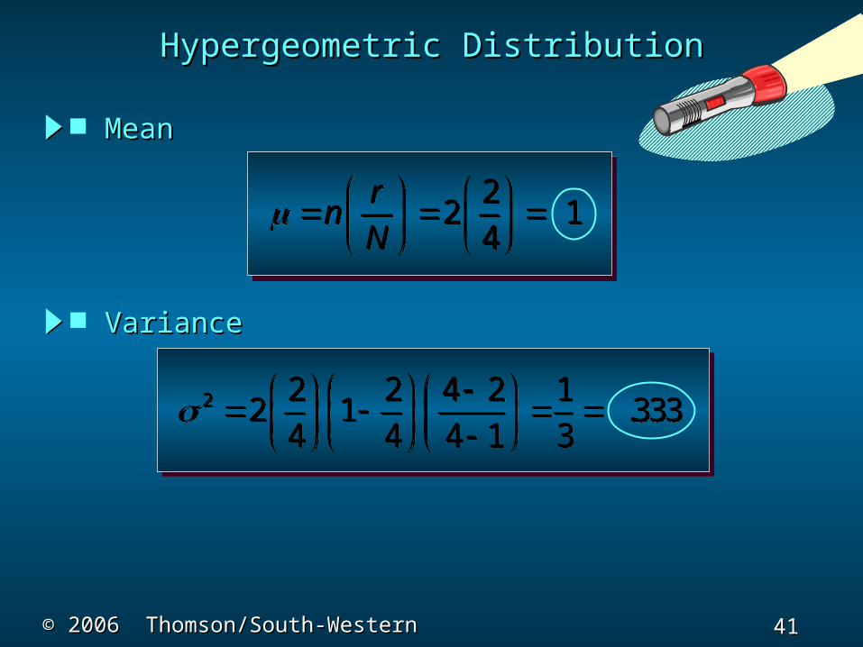
MeanMean
VarianceVariance
41 41 Slide
Slide
© 2006 Thomson/South-Western© 2006 Thomson/South-Western
Hypergeometric DistributionHypergeometric Distribution
22 1
4
rnN
22 1
4
rnN
2 2 2 4 2 12 1 .333
4 4 4 1 3
2 2 2 4 2 12 1 .333
4 4 4 1 3
MeanMean
VarianceVariance

42 42 Slide
Slide
© 2006 Thomson/South-Western© 2006 Thomson/South-Western
Hypergeometric DistributionHypergeometric Distribution
Consider a hypergeometric distribution with Consider a hypergeometric distribution with nn trials trials and let and let pp = ( = (rr//nn) denote the probability of a success) denote the probability of a success on the first trial.on the first trial.
If the population size is large, the term (If the population size is large, the term (NN – – nn)/()/(NN – 1) – 1) approaches 1.approaches 1.
The expected value and variance can be writtenhe expected value and variance can be written EE((xx) = ) = npnp and and VarVar((xx) = ) = npnp(1 – (1 – pp).).
Note that these are the expressions for the expectedhe expected value and variance of a binomial distribution.value and variance of a binomial distribution.
continuedcontinued

43 43 Slide
Slide
© 2006 Thomson/South-Western© 2006 Thomson/South-Western
Hypergeometric DistributionHypergeometric Distribution
When the population size is large, a hypergeometricWhen the population size is large, a hypergeometric distribution can be approximated by a binomialdistribution can be approximated by a binomial distribution with distribution with nn trials and a probability of success trials and a probability of success pp = ( = (rr//NN). ).
When the population size is large, a hypergeometricWhen the population size is large, a hypergeometric distribution can be approximated by a binomialdistribution can be approximated by a binomial distribution with distribution with nn trials and a probability of success trials and a probability of success pp = ( = (rr//NN). ).

44 44 Slide
Slide
© 2006 Thomson/South-Western© 2006 Thomson/South-Western
End of Chapter 5End of Chapter 5