slides prepared by john s. loucks - cameron universitycameron.edu/~syeda/orgl333/ch12.pdf · ©...

11SlideSlide©© 2006 Thomson/South2006 Thomson/South--WesternWestern

Slides Prepared by

JOHN S. LOUCKSSt. Edward’s University

Slides Prepared bySlides Prepared by

JOHN S. LOUCKSJOHN S. LOUCKSSt. EdwardSt. Edward’’s Universitys University


Chapter 12Chapter 12Simple Linear RegressionSimple Linear Regression

Simple Linear Regression ModelSimple Linear Regression ModelLeast Squares MethodLeast Squares MethodCoefficient of DeterminationCoefficient of DeterminationModel AssumptionsModel AssumptionsTesting for SignificanceTesting for SignificanceUsing the Estimated Regression EquationUsing the Estimated Regression Equation

for Estimation and Predictionfor Estimation and PredictionComputer SolutionComputer SolutionResidual Analysis: Validating Model AssumptionsResidual Analysis: Validating Model Assumptions


Simple Linear Regression ModelSimple Linear Regression Model

yy = = ββ00 + + ββ11xx ++εε

where:where:ββ00 and and ββ11 are called are called parameters of the modelparameters of the model,,εε is a random variable called theis a random variable called the error termerror term..

The The simple linear regression modelsimple linear regression model is:is:

The equation that describes how The equation that describes how yy is related to is related to xx andandan error term is called the an error term is called the regression modelregression model..


Simple Linear Regression EquationSimple Linear Regression Equation

The The simple linear regression equationsimple linear regression equation is:is:

•• EE((yy) is the expected value of ) is the expected value of yy for a given for a given xx value.value.•• ββ11 is the slope of the regression line.is the slope of the regression line.•• ββ00 is the is the yy intercept of the regression line.intercept of the regression line.•• Graph of the regression equation is a straight line.Graph of the regression equation is a straight line.

EE((yy) = ) = ββ00 + + ββ11xx



Positive Linear RelationshipPositive Linear Relationship

E(y)EE((yy))

xxx

Slope Slope ββ11is positiveis positive

Regression lineRegression line

InterceptInterceptββ00



Negative Linear RelationshipNegative Linear Relationship

E(y)EE((yy))

xxx

Slope Slope ββ11is negativeis negative

Regression lineRegression lineInterceptInterceptββ00



No RelationshipNo Relationship

E(y)EE((yy))

xxx

Slope Slope ββ11is 0is 0

Regression lineRegression lineInterceptIntercept

ββ00


Estimated Simple Linear Regression EquationEstimated Simple Linear Regression Equation

The The estimated simple linear regression equationestimated simple linear regression equation

0 1y b b x= +0 1y b b x= +

•• is the estimated value of is the estimated value of yy for a given for a given xx value.value.yy•• bb11 is the slope of the line.is the slope of the line.•• bb00 is the is the yy intercept of the line.intercept of the line.•• The graph is called the estimated regression line.The graph is called the estimated regression line.


Estimation ProcessEstimation Process

Regression ModelRegression Modelyy = = ββ00 + + ββ11xx ++εε

Regression EquationRegression EquationEE((yy) = ) = ββ00 + + ββ11xx

Unknown ParametersUnknown Parametersββ00, , ββ11

Sample Data:Sample Data:x x yyxx11 yy11. .. .. .. .

xxnn yynn

bb00 and and bb11provide estimates ofprovide estimates of

ββ00 and and ββ11

EstimatedEstimatedRegression EquationRegression Equation

Sample StatisticsSample Statisticsbb00, , bb11

0 1y b b x= +0 1y b b x= +


Least Squares MethodLeast Squares Method

Least Squares CriterionLeast Squares Criterion

min (y yi i−∑ )2min (y yi i−∑ )2

where:where:yyii = = observedobserved value of the dependent variablevalue of the dependent variable

for thefor the iithth observationobservation^yyii = = estimatedestimated value of the dependent variablevalue of the dependent variable

for thefor the iithth observationobservation


Slope for the Estimated Regression EquationSlope for the Estimated Regression Equation

1 2

( )( )( )

i i

i

x x y yb

x x− −

=−

∑∑1 2

( )( )( )

i i

i

x x y yb

x x− −

=−

∑∑



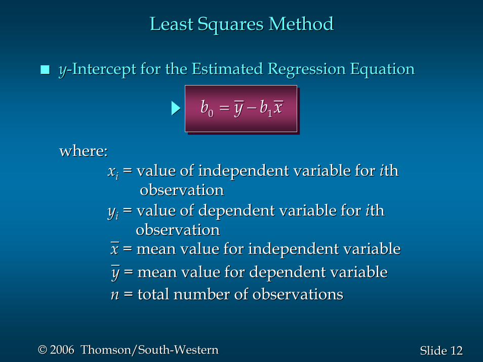
yy--Intercept for the Estimated Regression EquationIntercept for the Estimated Regression Equation


0 1b y b x= −0 1b y b x= −

where:where:xxii = value of independent variable for = value of independent variable for iithth

observationobservation

nn = total number of observations= total number of observations

__yy = mean value for dependent variable= mean value for dependent variable

__xx = mean value for independent variable= mean value for independent variable

yyii = value of dependent variable for= value of dependent variable for iiththobservationobservation


Reed Auto periodically hasReed Auto periodically hasa special weeka special week--long sale. long sale. As part of the advertisingAs part of the advertisingcampaign Reed runs one orcampaign Reed runs one ormore television commercialsmore television commercialsduring the weekend preceding the sale. Data from aduring the weekend preceding the sale. Data from asample of 5 previous sales are shown on the next slide.sample of 5 previous sales are shown on the next slide.

Simple Linear RegressionSimple Linear Regression

Example: Reed Auto SalesExample: Reed Auto Sales


Simple Linear RegressionSimple Linear Regression

Example: Reed Auto SalesExample: Reed Auto Sales

Number ofNumber ofTV AdsTV Ads

Number ofNumber ofCars SoldCars Sold

1133221133

14142424181817172727


Estimated Regression EquationEstimated Regression Equation

ˆ 10 5y x= +ˆ 10 5y x= +

1 2

( )( ) 20 5( ) 4

i i

i

x x y yb

x x− −

= = =−

∑∑1 2

( )( ) 20 5( ) 4

i i

i

x x y yb

x x− −

= = =−

∑∑

0 1 20 5(2) 10b y b x= − = − =0 1 20 5(2) 10b y b x= − = − =

yy--Intercept for the Estimated Regression EquationIntercept for the Estimated Regression Equation

Slope for the Estimated Regression EquationSlope for the Estimated Regression Equation

Estimated Regression EquationEstimated Regression Equation


Scatter Diagram and Trend LineScatter Diagram and Trend Line

y = 5x + 10

0

5

10

15

20

25

30

0 1 2 3 4TV Ads

Car

s So

ld


Coefficient of DeterminationCoefficient of Determination

Relationship Among SST, SSR, SSERelationship Among SST, SSR, SSE

where:where:SST = total sum of squaresSST = total sum of squaresSSR = sum of squares due to regressionSSR = sum of squares due to regressionSSE = sum of squares due to errorSSE = sum of squares due to error

SST = SST = SSR SSR + + SSESSE

2( )iy y−∑ 2( )iy y−∑ 2ˆ( )iy y= −∑ 2ˆ( )iy y= −∑ 2ˆ( )i iy y+ −∑ 2ˆ( )i iy y+ −∑


The The coefficient of determinationcoefficient of determination is:is:


where:where:SSR = sum of squares due to regressionSSR = sum of squares due to regressionSST = total sum of squaresSST = total sum of squares

rr22 = SSR/SST= SSR/SST



rr22 = SSR/SST = 100/114 = .8772= SSR/SST = 100/114 = .8772

The regression relationship is very strong; 88%The regression relationship is very strong; 88%of the variability in the number of cars sold can beof the variability in the number of cars sold can beexplained by the linear relationship between theexplained by the linear relationship between thenumber of TV ads and the number of cars sold.number of TV ads and the number of cars sold.


Sample Correlation CoefficientSample Correlation Coefficient

21 ) of(sign rbrxy = 21 ) of(sign rbrxy =

ionDeterminat oft Coefficien ) of(sign 1brxy = ionDeterminat oft Coefficien ) of(sign 1brxy =

where:where:bb11 = the slope of the estimated regression= the slope of the estimated regression

equationequation xbby 10ˆ += xbby 10ˆ +=


21 ) of(sign rbrxy = 21 ) of(sign rbrxy =

The sign of The sign of bb11 in the equationin the equation is is ““++””..ˆ 10 5y x= +ˆ 10 5y x= +

= + .8772xyr = + .8772xyr

Sample Correlation CoefficientSample Correlation Coefficient

rrxyxy = +.9366= +.9366


Assumptions About the Error Term Assumptions About the Error Term εε

1. The error ε is a random variable with mean of zero.1. The error 1. The error εε is a random variable with mean of zero.is a random variable with mean of zero.

2. The variance of ε , denoted by σ 2, is the same forall values of the independent variable.

2. The variance of 2. The variance of εε , denoted by , denoted by σσ 22, is the same for, is the same forall values of the independent variable.all values of the independent variable.

3. The values of ε are independent.3. The values of 3. The values of εε are independent.are independent.

4. The error ε is a normally distributed randomvariable.

4. The error 4. The error εε is a normally distributed randomis a normally distributed randomvariable.variable.


Testing for SignificanceTesting for Significance

To test for a significant regression relationship, wemust conduct a hypothesis test to determine whetherthe value of β1 is zero.

To test for a significant regression relationship, weTo test for a significant regression relationship, wemust conduct a hypothesis test to determine whethermust conduct a hypothesis test to determine whetherthe value of the value of ββ11 is zero.is zero.

Two tests are commonly used:Two tests are commonly used:Two tests are commonly used:

tt TestTest andand FF TestTest

Both the t test and F test require an estimate of σ 2,the variance of ε in the regression model.Both the Both the tt test and test and FF test require an estimate of test require an estimate of σσ 22,,the variance of the variance of εε in the regression model.in the regression model.


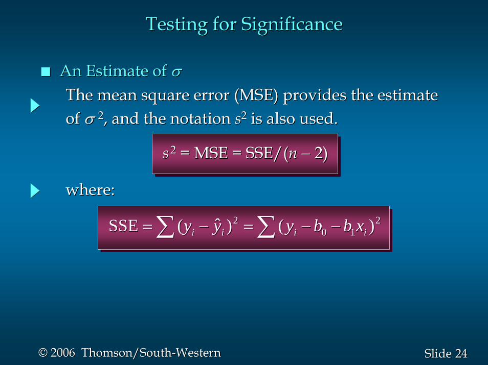
An Estimate of An Estimate of σσ


∑∑ −−=−= 210

2 )()ˆ(SSE iiii xbbyyy ∑∑ −−=−= 210

2 )()ˆ(SSE iiii xbbyyy

where:where:

ss 22 = MSE = SSE/(= MSE = SSE/(n n −− 2)2)

The mean square error (MSE) provides the estimateThe mean square error (MSE) provides the estimateof of σσ 22, and the notation , and the notation ss22 is also used.is also used.



An Estimate of An Estimate of σσ

2SSEMSE

−==

ns

2SSEMSE

−==

ns

•• To estimate To estimate σσ we take the square root of we take the square root of σ σ 22..

•• The resulting The resulting ss is called the is called the standard error ofstandard error ofthe estimatethe estimate..


HypothesesHypotheses

Test StatisticTest Statistic

Testing for Significance: Testing for Significance: tt TestTest

0 1: 0H β =0 1: 0H β =

1: 0aH β ≠1: 0aH β ≠

1

1

b

bts

=1

1

b

bts

=


Rejection RuleRejection Rule


where: where: ttα/α/22 is based on a is based on a tt distributiondistributionwith with nn -- 2 degrees of freedom2 degrees of freedom

Reject Reject HH00 if if pp--value value << ααor or tt << --ttα/α/2 2 or or tt >> ttα/α/2 2


1. Determine the hypotheses.1. Determine the hypotheses.

2. Specify the level of significance.2. Specify the level of significance.

3. Select the test statistic.3. Select the test statistic.

α α = .05= .05

4. State the rejection rule.4. State the rejection rule. Reject Reject HH00 if if pp--value value << .05.05or |or |t|t| > 3.182 (with> 3.182 (with

3 degrees of freedom)3 degrees of freedom)


0 1: 0H β =0 1: 0H β =

1: 0aH β ≠1: 0aH β ≠

1

1

b

bts

=1

1

b

bts

=



5. Compute the value of the test statistic.5. Compute the value of the test statistic.

6. Determine whether to reject 6. Determine whether to reject HH00..

tt = 4.541 provides an area of .01 in the upper= 4.541 provides an area of .01 in the uppertail. Hence, the tail. Hence, the pp--value is less than .02. (Also,value is less than .02. (Also,tt = 4.63 > 3.182.) We can reject = 4.63 > 3.182.) We can reject HH00..

1

1 5 4.631.08b

bts

= = =1

1 5 4.631.08b

bts

= = =


Confidence Interval for Confidence Interval for ββ11

HH00 is rejected if the hypothesized value of is rejected if the hypothesized value of ββ11 is notis notincluded in the confidence interval for included in the confidence interval for ββ11..

We can use a 95% confidence interval for We can use a 95% confidence interval for ββ11 to testto testthe hypotheses just used in the the hypotheses just used in the tt test.test.


The form of a confidence interval for The form of a confidence interval for ββ11 is:is:


11 /2 bb t sα±11 /2 bb t sα±

wherewhere is the is the tt value providing an areavalue providing an areaof of αα/2 in the upper tail of a /2 in the upper tail of a tt distributiondistributionwith with n n -- 2 degrees of freedom2 degrees of freedom

2/αt 2/αtbb11 is theis the

pointpointestimatorestimator

is theis themarginmarginof errorof error

1/2 bt sα 1/2 bt sα



Reject Reject HH00 if 0 is not included inif 0 is not included inthe confidence interval for the confidence interval for ββ11..

0 is not included in the confidence interval. 0 is not included in the confidence interval. Reject Reject HH00

= 5 +/= 5 +/-- 3.182(1.08) = 5 +/3.182(1.08) = 5 +/-- 3.443.4412/1 bstb α±12/1 bstb α±

or 1.56 to 8.44or 1.56 to 8.44


95% Confidence Interval for 95% Confidence Interval for ββ11

ConclusionConclusion


HypothesesHypotheses

Test StatisticTest Statistic

FF = MSR/MSE= MSR/MSE

0 1: 0H

Testing for Significance: Testing for Significance: FF TestTest

β =0 1: 0H β =

1: 0aH β ≠1: 0aH β ≠



Reject Reject HH00 ififpp--value value <<


where:where:FFαα is based on an is based on an FF distribution withdistribution with1 degree of freedom in the numerator and1 degree of freedom in the numerator andnn -- 2 degrees of freedom in the denominator2 degrees of freedom in the denominator

ααor or FF >> FFαα


1. Determine the hypotheses.1. Determine the hypotheses.

2. Specify the level of significance.2. Specify the level of significance.

3. Select the test statistic.3. Select the test statistic.

α α = .05= .05

4. State the rejection rule.4. State the rejection rule. Reject Reject HH00 if if pp--value value << .05.05or or FF >> 10.13 (with 10.13 (with 1 d.f.1 d.f.

in numerator andin numerator and3 d.f. in denominator)3 d.f. in denominator)


0 1: 0H β =0 1: 0H β =

1: 0aH β ≠1: 0aH β ≠

FF = MSR/MSE= MSR/MSE



5. Compute the value of the test statistic.5. Compute the value of the test statistic.

6. Determine whether to reject 6. Determine whether to reject HH00..

FF = 17.44 provides an area of .025 in the upper = 17.44 provides an area of .025 in the upper tail. Thus, the tail. Thus, the pp--value corresponding to value corresponding to FF = 21.43 = 21.43 is less than 2(.025) = .05. Hence, we reject is less than 2(.025) = .05. Hence, we reject HH00..

FF = MSR/MSE = 100/4.667 = 21.43= MSR/MSE = 100/4.667 = 21.43

The statistical evidence is sufficient to concludeThe statistical evidence is sufficient to concludethat we have a significant relationship between thethat we have a significant relationship between thenumber of TV ads aired and the number of cars sold. number of TV ads aired and the number of cars sold.


Some Cautions about theSome Cautions about theInterpretation of Significance TestsInterpretation of Significance Tests

Just because we are able to reject Just because we are able to reject HH00: : ββ11 = 0 and= 0 anddemonstrate statistical significance does not enabledemonstrate statistical significance does not enableus to conclude that there is a us to conclude that there is a linear relationshiplinear relationshipbetween between xx and and yy..

Rejecting Rejecting HH00: : ββ11 = 0 and concluding that the= 0 and concluding that therelationship between relationship between xx and and yy is significant does is significant does not enable us to conclude that a not enable us to conclude that a causecause--andand--effecteffectrelationshiprelationship is present between is present between xx and and yy..


Using the Estimated Regression EquationUsing the Estimated Regression Equationfor Estimation and Predictionfor Estimation and Prediction

/y t sp yp± α 2/y t sp yp± α 2

where:where:confidence coefficient is 1 confidence coefficient is 1 -- αα andandttαα/2 /2 is based on ais based on a t t distributiondistributionwith with nn -- 2 degrees of freedom2 degrees of freedom

/2 indpy t sα± /2 indpy t sα±

Confidence Interval Estimate of Confidence Interval Estimate of EE((yypp))

Prediction Interval Estimate of Prediction Interval Estimate of yypp


If 3 TV ads are run prior to a sale, we expectIf 3 TV ads are run prior to a sale, we expectthe mean number of cars sold to be:the mean number of cars sold to be:

Point EstimationPoint Estimation

^yy = 10 + 5(3) = 25 cars= 10 + 5(3) = 25 cars


ExcelExcel’’s Confidence Interval Outputs Confidence Interval Output D E F G1 CONFIDENCE INTERVAL2 x p 33 xbar 2.04 x p -xbar 1.05 (x p -xbar)2 1.06 Σ (x p -xbar)2 4.07 Variance of yhat 2.10008 Std. Dev of yhat 1.44919 t Value 3.1824

10 Margin of Error 4.611811 Point Estimate 25.012 Lower Limit 20.3913 Upper Limit 29.61

Confidence Interval for Confidence Interval for EE((yypp))


The 95% confidence interval estimate of the mean The 95% confidence interval estimate of the mean number of cars sold when 3 TV ads are run is:number of cars sold when 3 TV ads are run is:

Confidence Interval for Confidence Interval for EE((yypp))

25 25 ++ 4.61 = 20.39 to 29.61 cars4.61 = 20.39 to 29.61 cars


ExcelExcel’’s Prediction Interval Outputs Prediction Interval Output H I1 PREDICTION INTERVAL2 Variance of y ind 6.766673 Std. Dev. of y ind 2.601284 Margin of Error 8.278455 Lower Limit 16.726 Upper Limit 33.287

Prediction Interval for Prediction Interval for yypp


The 95% prediction interval estimate of the The 95% prediction interval estimate of the number of cars sold in one particular week when 3 number of cars sold in one particular week when 3 TV ads are run is:TV ads are run is:

Prediction Interval for Prediction Interval for yypp

25 25 ++ 8.28 = 16.72 to 33.28 cars8.28 = 16.72 to 33.28 cars


Residual AnalysisResidual Analysis

ˆi iy y− ˆi iy y−

Much of the residual analysis is based on anMuch of the residual analysis is based on anexamination of graphical plots.examination of graphical plots.

Residual for Observation Residual for Observation iiThe residuals provide the best information about The residuals provide the best information about εε ..

If the assumptions about the error term If the assumptions about the error term εε appearappearquestionable, the hypothesis tests about thequestionable, the hypothesis tests about thesignificance of the regression relationship and thesignificance of the regression relationship and theinterval estimation results may not be valid.interval estimation results may not be valid.


Residual Plot Against Residual Plot Against xx

If the assumption that the variance of If the assumption that the variance of εε is the same is the same for all values of for all values of x x is valid, and the assumed is valid, and the assumed regression model is an adequate representation of the regression model is an adequate representation of the relationship between the variables, thenrelationship between the variables, then

The residual plot should give an overallThe residual plot should give an overallimpression of a horizontal band of pointsimpression of a horizontal band of points


xx

ˆy y− ˆy y−

00

Good PatternGood PatternRe

sidu

alRe

sidu

al




xx

ˆy y− ˆy y−

00

Resi

dual

Resi

dual

NonconstantNonconstant VarianceVariance



xx

ˆy y− ˆy y−

00

Resi

dual

Resi

dual

Model Form Not AdequateModel Form Not Adequate


ResidualsResiduals

Observation Predicted Cars Sold Residuals1 15 -12 25 -13 20 -24 15 25 25 2




TV Ads Residual Plot

-3

-2

-1

0

1

2

3

0 1 2 3 4TV Ads

Resi

dual

s


End of Chapter 12End of Chapter 12

slides prepared by john s. loucks - cameron universitycameron.edu/~syeda/orgl333/ch12.pdf · ©...

Documents