slides complements-flows

Arthur Charpentier, Master Statistique & Économétrie - Université Rennes 1 - 2017

Maps and Projections

Source: explainxkcd.com

@freakonometrics freakonometrics freakonometrics.hypotheses.org 1

http://www.explainxkcd.com/wiki/index.php/977:_Map_Projections

https://twitter.com/freakonometrics

https://freakonometrics.github.io/

https://freakonometrics.hypotheses.org/



1 library ( rgdal )

2 library ( maptools )

3 Proj <- CRS("+proj= longlat + datum = WGS84 ")

4 CAN_shp <- readShapePoly ("CAN_adm1.shp",

verbose =TRUE , proj4string =Proj)

5 plot(CAN_shp)

6 new_CAN_shp <- spTransform (CAN_shp , CRS("+

init=epsg :26978 "))

7 plot(new_CAN_shp)







1 library (sp)

2 library ( rworldmap )

3 data( countriesLow )

4 crs. WGS84 <- CRS("+proj= longlat + datum = WGS84

")

5 countries . WGS84 <- spTransform ( countriesLow ,

crs. WGS84 )

6 plot( countries .WGS84 ,col=" light green ")

7 crs.laea <- CRS("+proj=laea +lat_0=52 +lon_

0=10 +x_ 0=4321000 +y_ 0=3210000 + ellps =

GRS80 + units =m +no_defs")

8 countries .laea <- spTransform ( countriesLow ,

crs.laea)

9 plot( countries .laea ,col=" light green ")






Maps and Points1 library (maps)

2 data(" world . cities ")

3 world . cities2 = world . cities [ world . cities $pop >100000 ,]

4 plot( world . cities2 $lon , world . cities2 $lat ,pch =19 , cex =.7 , axes=FALSE ,

xlab="",ylab="")






Maps and Lines1 loc=" https ://raw. githubusercontent .com/ jjrom / hydre / master / mapserver /

geodata / rivers /GRDC_687_ rivers "

2 ext=c(".dbf",".prj",".sbn",".sbx",".shp",".shp.xml",".shx")

3 dir. create (’data/ rivieres ’)

4 for(i in 1: length (ext)){

5 loc1= paste (loc ,ext[i],"?raw=true",sep="")

6 loc2= paste ("data/ rivieres /GRDC_687_ rivers ",ext[i],sep="")

7 getdata (loc1 ,loc2)

8 }






Maps and Lines1 library ("sp")

2 library (" rgdal ")

3 shape <- readShapeLines ("GRDC_687_ rivers .shp")

4 plot(shape ,col="blue")






Maps and Lines1 crs.laea <- CRS("+proj=laea +lat_0=52 +lon_0=10 +x_ 0=4321000 +y_

0=3210000 + ellps = GRS80 + units =m +no_defs")

2 shape . nouveau = spTransform (shape ,crs.laea)

3 plot( shape .nouveau ,col="blue")






Maps and Lines1 getdatazip ("http://www. naturalearthdata .com/http//www.

naturalearthdata .com/ download /10m/ cultural /ne_10m_ roads .zip", "

data/ routes .zip", ’data/ routes /’)

2 shape <- readShapeLines ("data/ routes /ne_10m_ roads .shp")

3 plot(shape ,pch =19 , lwd =.7)






Maps and Polygons

1 download .file("http:// freakonometrics .free.

fr/ Italy .zip",destfile =" Italy .zip")

2 library ( rgdal )

3 ita1 <-readOGR (dsn="/ Italy ",layer ="ITA_adm1",

verbose = FALSE )

4 plot(ita1 ,col=" light green ")






Maps and Polygons

1 > ita1@data [,"NAME_1" ][1:6]

2 [1] Abruzzo Apulia Basilicata Calabria

3 [5] Campania Emilia - Romagna

4 pos <-which ( ita1@data [,"NAME_1"]==" Sicily ")

5 Poly_ Sicily <-ita1[pos ,]


7 plot(Poly_Sicily ,col=" yellow ",add=TRUE)






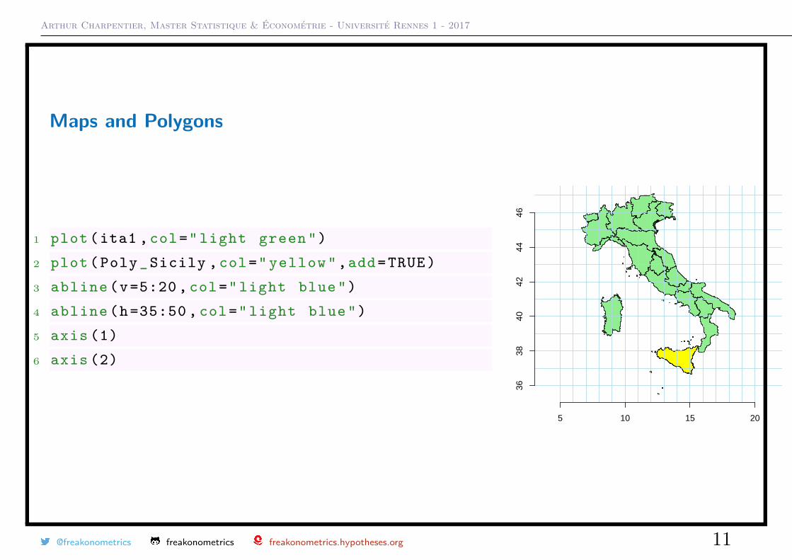
Maps and Polygons



3 abline (v=5:20 , col=" light blue")

4 abline (h=35:50 , col=" light blue")

5 axis (1)

6 axis (2)

5 10 15 20

3638

4042

4446






Maps and Polygons

1 pos <-which ( ita1@data [,"NAME_1"] %in% c("

Abruzzo "," Apulia "," Basilicata "," Calabria

"," Campania "," Lazio "," Molise "," Sardegna "

," Sicily "))

2 ita_ south <- ita1[pos ,]

3 ita_ north <- ita1[-pos ,]

4 plot(ita1)

5 plot(ita_south ,col="red",add=TRUE)

6 plot(ita_north ,col="blue",add=TRUE)






Maps and Polygons

Here we have only used colors, but it is also possible to merge the polygonstogether,

1 library ( rgeos )

2 ita_s<- gUnionCascaded (ita_ south )

3 ita_n<- gUnionCascaded (ita_ north )

4 plot(ita1)

5 plot(ita_s,col="red",add=TRUE)

6 plot(ita_n,col="blue",add=TRUE)






Maps and Polygons

On polygons, it is also possible to visualize centroids,



3 > gCentroid (Poly_Sicily ,byid=TRUE)

4 SpatialPoints :

5 x y

6 14 14.14668 37.58842

7 Coordinate Reference System (CRS) arguments :

8 +proj= longlat + ellps = WGS84

9 + datum = WGS84 +no_defs + towgs84 =0 ,0 ,0

10 points ( gCentroid (Poly_Sicily ,byid=TRUE),pch

=19 , col="red")

●






Maps and Polygons or

1 G <- as.data. frame ( gCentroid (ita1 ,byid=TRUE)

)


3 text(G$x,G$y ,1:20)

1

23

4

5

6

7

8

9

10

11

12

13

14

15

16

17

18

19 20






Maps and Polygons

Consider two trajectories, caracterized by a series of knots (from the centroïdslist)

1 c1 <-G[c(17 ,20 ,6 ,16 ,8 ,12 ,2) ,]

2 c2 <- G[c(13 ,11 ,1 ,5 ,3 ,4) ,]

We can convert those segments into SpatialLines3 L1 <-SpatialLines (list( Lines (list(Line(c1))," Line1 ")))

4 L2 <-SpatialLines (list( Lines (list(Line(c2))," Line2 ")))

To make sure that we can add those lines on the map, use






3 L1@proj4string <- ita1@proj4string

4 L2@proj4string <- ita1@proj4string

5 cross _road <- gIntersection (L1 ,L2)

6 > cross _ road@coords

7 SpatialPoints :

8 x y

9 1 11.06947 44.03287

10 1 14.20034 41.74879

11 Coordinate Reference System (CRS) arguments :

12 +proj= longlat + ellps = WGS84

13 + datum = WGS84 +no_defs + towgs84 =0 ,0 ,0


15 plot(L1 ,col="red",lwd =2, add=TRUE)

16 plot(L2 ,col="blue",lwd =2, add=TRUE)

17 plot( cross _road ,pch =19 , cex =1.5 , add=TRUE)






Maps and Polygons

To add elements on maps, consider, e.g.


2 grat <- border _plot(sp=ita1 ,WE=seq (5 ,20 , by

=2.5) ,NS=seq (36 ,47))

3 plot(grat ,col=" light blue",add=TRUE)

4 labs <-paste (seq (5 ,20 , by =2.5) ," E",sep="")

5 axis(side =1, pos =36 , at=seq (5 ,20 , by =2.5) ,

6 labels =labs)

7 axis(side =3, pos =47 , at=seq (5 ,20 , by =2.5) ,

8 labels =labs)

9 labs <-paste (seq (36 ,47) ," N",sep="")

10 axis(side =2, pos =5,at=seq (36 ,47) ,

11 labels =labs)

12 axis(side =4, pos =20 , at=seq (36 ,47) ,

13 labels =labs)

5 E 7.5 E 10 E 12.5 E 15 E 17.5 E 20 E

5 E 7.5 E 10 E 12.5 E 15 E 17.5 E 20 E

36 N

38 N

40 N

42 N

44 N

46 N

36 N

38 N

40 N

42 N

44 N

46 N






Maps and Polygons

To add elements on maps, consider, e.g.

1 sea <-data. frame (Name=c(" MEDITERANEAN \nSEA","

ADRIATIC \nSEA"," IONIAN \nSEA"),

2 Longitude =c (7.5 ,16.25 ,18.25) ,Latitude =c

(37.5 ,44.5 ,38.5) )

3 text(sea$Longitude ,sea$Latitude ,sea$Name ,

4 cex =0.75 , col="#34 bdf2",font =3)

5 library ( raster )

6 scalebar (d=500 , xy=c (5.25 ,36.5) ,,type="bar",

below ="km",

7 lwd =4, divs =2, col=" black ",cex =0.75 , lonlat =

TRUE)5 E 7.5 E 10 E 12.5 E 15 E 17.5 E 20 E

5 E 7.5 E 10 E 12.5 E 15 E 17.5 E 20 E

36 N

38 N

40 N

42 N

44 N

46 N

36 N

38 N

40 N

42 N

44 N

46 N

MEDITERANEANSEA

ADRIATICSEA

IONIANSEA

0 500km






Maps and Polygons

1 library (sp)

2 library ( raster )

3 download .file("http:// biogeo . ucdavis .edu/

data/ gadm2 .8/rds/GBR_adm2.rds","GBR_adm2

.rds")

4 UK= readRDS ("GBR_adm2.rds")

5 UK@data [159 ,"HASC_2"]="GB.NR"

6 plot(UK , xlim = c(-4,-2), ylim = c(50 , 59) ,

main="UK areas ")






Maps and Polygons

One can add Ireland on the left part1 download .file("http:// biogeo . ucdavis .edu/

data/ gadm2 .8/rds/IRL_adm0.rds","IRL_adm0

.rds")

2 IRL= readRDS ("IRL_adm0.rds")

3 plot(IRL ,add=TRUE)






Maps and Polygonsand France, in the lower right corner

1 download .file("http:// biogeo . ucdavis .edu/

data/ gadm2 .8/rds/FRA_adm0.rds","FRA_adm0

.rds")

2 FR= readRDS ("FRA_adm0.rds")

3 plot(FR ,add=TRUE)

4 loc=" https ://f. hypotheses .org/wp - content /

blogs .dir/253/ files /2016/12/EU -

referendum -result -data.csv"

5 referendum =read.csv(loc , header =TRUE ,dec=".",

sep=",",stringsAsFactors = FALSE )

6 referendum = referendum [c(3 ,6 ,13 ,14)]

7 library (plyr)

8 referendum = ddply ( referendum ,.( Region ,HASC_

code),summarise , Remain =sum( Remain ),Leave

=sum( Leave ))






Maps and Polygons1 row. names ( referendum )=seq (1, nrow( referendum ) ,1)

2 leave _or_ remain = cbind ( referendum ," Brexit ?"=0)

3 leave _or_ remain [," Brexit ?"]= ifelse ( leave _or_ remain $

Remain < leave _or_ remain $Leave ,rgb (1 ,0 ,0 ,.7) ,rgb

(0 ,0 ,1 ,.7))

4 map_data=data. frame ( UK@data )

5 map_data= cbind (map_data ," Brexit "=0)

6 for (i in 1: nrow(map_data)){

7 if(map_data[i,"NAME_1"]==" Northern Ireland "){

8 map_data[i," Brexit "]="blue"}else{

9 map_data[i," Brexit "]= as. character ( leave _or_ remain [

leave _or_ remain $HASC_code == map_data$HASC_2[i],’

Brexit ?’]) }}

10 plot(UK , col = map_data$Brexit , border = " gray1 ",

xlim = c(-4,-2), ylim = c(50 , 59) , main="How the

UK has voted ?", bg="# A6CAE0 ")

11 plot(IRL , col = " lightgrey ", border = " gray1 ",add=

TRUE)@freakonometrics freakonometrics freakonometrics.hypotheses.org 23





Maps and Polygons

1 library ( cartography )

2 cols <- carto .pal(pal1 = "red.pal",n1 = 5,pal2="

green .pal",n2 =5)

3 map_data=data. frame ( UK@data )

4 map_data= cbind (map_data ," Percentage _ Remain "=0)

5 for (i in 1: nrow(map_data)){

6 if(map_data[i,"NAME_1"]==" Northern Ireland "){

7 map_data[i," Percentage _ Remain " ]=55.78} else{

map_data[i," Percentage _ Remain " ]=100 * leave _or_

remain [ leave _or_ remain $HASC_code == map_data$HASC_

2[i]," Remain "]/( leave _or_ remain [ leave _or_ remain $

HASC_code == map_data$HASC_2[i]," Remain "]+ leave _or_

remain [ leave _or_ remain $HASC_code == map_data$HASC_

2[i]," Leave "]) }}

(... to be continued)






Maps and Polygons

1 plot(UK , col = "grey", border = " gray1 ", xlim = c

(-4,-2), ylim = c(50 , 59) ,bg="# A6CAE0 ")

2 plot(IRL , col = " lightgrey ", border = " gray1 ",add=

TRUE)

3 plot(FR , col = " lightgrey ", border = " gray1 ",add=

TRUE)

4 choroLayer (spdf = UK ,

5 df = map_data ,

6 var = " Percentage _ Remain ",

7 breaks = seq (0 ,100 ,10) ,

8 col = cols ,

9 legend .pos = " topright ",

10 legend . title .txt = "",

11 legend . values .rnd = 2,

12 add = TRUE)







1 library ( maptools )

2 library ( rgdal )

3 library ( PBSmapping )

4 download .file("http:// freakonometrics .free.

fr/paris - cartelec .zip","paris - cartelec .

zip")

5 unzip ("paris - cartelec .zip")

6 paris <- readShapeSpatial ( "paris - cartelec .

shp" )

7 proj4string ( paris ) <- CRS( "+init=epsg

:2154 " )

8 paris <- spTransform ( paris , CRS( "+proj=

longlat + ellps = GRS80 " ) )

9 plot ( paris )







1 point =c (2.33 ,48.849)

2 plot(point ,xlim= point [1]+c( -.01 ,.01) ,ylim=

point [2]+c( -.01 ,.01))

3 plot(paris ,add=TRUE)

4

5 library ( rgeos )

6 idx= unique (poly_ paris $PID)

7 for(i in idx){

8 ct= centroid (as. matrix (poly_ paris [poly_ paris $

PID ==i,c("X","Y")]))

9 text(ct [1] , ct [2] ,i,col="blue")}







1 which .poly <- function ( point ) {

2 idx= unique (poly_ paris $PID)

3 idx_ valid =NULL

4 for ( i in idx ) {

5 pip= point .in. polygon ( point [ 1 ] , point [ 2

] ,

6 poly_ paris [ poly_ paris $PID ==i , "X" ] ,

7 poly_ paris [ poly_ paris $PID ==i , "Y" ] )

8 if ( pip >0) idx_ valid =c ( idx_ valid , i )

}

9 return ( idx_ valid ) }

Hence, here10 > which .poly( point )

11 [1] 86






Using Google Maps and Open Street Maps1 library ( ggmap )

2 library ( geosphere )

3 > ( Hotel <- geocode ("8 sinaran drive singapore "))

4 Information from URL : http://maps. googleapis .com/maps/api/ geocode /

json? address =8+ sinaran + drive + singapore & sensor = false

5 Google Maps API Terms of Service : http:// developers . google .com/maps/

terms

6 lon lat

7 1 103.845 1.320279

8 > ( Airport <- geocode (" singapore airport "))

9 Information from URL : http://maps. googleapis .com/maps/api/ geocode /

json? address = singapore + airport & sensor = false

10 Google Maps API Terms of Service : http:// developers . google .com/maps/

terms

11 lon lat

12 1 103.9915 1.36442






Using Google Maps and Open Street Maps

The distance, in km, is obtained using the Haversine formula wikipedia.org1 > distHaversine (Airport ,Hotel , r =6378.137)

2 [1] 17.03514

while the driving distance is1 > mapdist (as. numeric ( Hotel ),as. numeric ( Airport ))

2 from to

m km miles

3 1 8 Sinaran Dr , Singapore 307470 80 Airport Blvd , Singapore 819642

19627 19.627 12.19622

4 seconds minutes hours

5 1 1220 20.33333 0.3388889


http://en.wikipedia.org/wiki/Haversine_formula





Background Maps

1 Loc=data. frame ( rbind (Airport , Hotel ))

2 library ( ggmap )

3 library ( RgoogleMaps )

4 CenterOfMap <- as.list( apply (Loc ,2, mean))

5 SG <- get_map(c(lon= CenterOfMap $lon , lat=

CenterOfMap $lat),zoom = 11, maptype = "

terrain ", source = " google ")

6 SGMap <- ggmap (SG)

7 SGMap

or1 SGMap <- get_map(c(lon= CenterOfMap $lon , lat=


roadmap ")

2 ggmap ( SGMap )

1.2

1.3

1.4

1.5

103.7 103.8 103.9 104.0 104.1lon

lat

1.2

1.3

1.4

1.5

103.7 103.8 103.9 104.0 104.1lon

lat






Background Maps

Note that those are ggplot2 maps, see ggmapCheat-sheet

1 SGMap <- get_map(c(lon= CenterOfMap $lon , lat=


satellite ")

2 ggmap ( SGMap )

or1 SGMap <- get_map(c(lon= CenterOfMap $lon , lat=


toner ", source = " stamen ")

2 ggmap ( SGMap )

1.2

1.3

1.4

1.5

103.7 103.8 103.9 104.0 104.1lon

lat

1.2

1.3

1.4

1.5

103.7 103.8 103.9 104.0 104.1lon

lat


https://www.nceas.ucsb.edu/~frazier/RSpatialGuides/ggmap/ggmapCheatsheet.pdf

https://www.nceas.ucsb.edu/~frazier/RSpatialGuides/ggmap/ggmapCheatsheet.pdf





Background Maps

1 library ( OpenStreetMap )

2 map <- openmap (c(lat= 51.516 , lon= -.141) ,

c(lat= 51.511 , lon= -.133))

3 map <- openproj (map , projection = "+init=

epsg :27700 ")

4 plot(map)






Background Maps

1 library ( OpenStreetMap , verbose =FALSE , quietly =

TRUE ,warn. conflicts = FALSE )

2 map <- openmap (c(lat= 51.516 , lon= -.141) , c

(lat= 51.511 , lon= -.133))

3 map <- openproj (map , projection = "+init=

epsg :27700 ")

4 plot(map)

5 loc="http:// freakonometrics .free.fr/ cholera .

zip"

6 download .file(loc , destfile =" cholera .zip")

7 unzip (" cholera .zip", exdir ="./")

8 library (maptools , verbose =FALSE , quietly =TRUE ,

warn. conflicts = FALSE )

9 deaths <- readShapePoints (" Cholera _ Deaths ")






Background Maps

1 head( deaths@coords )

2 ## coords .x1 coords .x2

3 ## 0 529309 181031

4 ## 1 529312 181025

5 ## 2 529314 181020

6 ## 3 529317 181014

7 ## 4 529321 181008

8 ## 5 529337 181006

9 plot(map)

10 points ( deaths@coords ,col="red", pch =19 , cex

=.7 )






Background Maps

1 X = deaths@coords

2 library ( KernSmooth )

3 kde2d = bkde2D (X, bandwidth =c(bw.ucv(X[ ,1]) ,

bw.ucv(X[ ,2])))

4 library (grDevices , verbose =FALSE , quietly =TRUE

,warn. conflicts = FALSE )

5 clrs = colorRampPalette (c(rgb (0 ,0 ,1 ,0) , rgb

(0 ,0 ,1 ,1)), alpha = TRUE)(20)

6 plot(map)

7 points ( deaths@coords ,col="red", pch =19 , cex

=.7 )

8 image (x= kde2d $x1 , y= kde2d $x2 ,z= kde2d $fhat ,

add=TRUE ,col=clrs)

9 contour (x= kde2d $x1 , y= kde2d $x2 ,z= kde2d $fhat ,

add=TRUE)






Background Maps

or one can use a ggplot2 visualization with Google Maps,

1 library (ggmap , verbose =FALSE , quietly =TRUE ,


2 get_ london = get_map(c ( -.137 ,51.513) , zoom

=17)

3 london = ggmap (get_ london )

4 london


https://journal.r-project.org/archive/2013-1/kahle-wickham.pdf





Background Maps

1 df_ deaths <- data. frame (X)

2 library (sp , verbose =FALSE , quietly =TRUE ,warn.

conflicts = FALSE )

3 library (rgdal , verbose =FALSE , quietly =TRUE ,


4 coordinates (df_ deaths )=~ coords .x1+ coords .x2

5 proj4string (df_ deaths )=CRS("+init=epsg :27700

")

6 df_ deaths = spTransform (df_deaths ,CRS("+proj

= longlat + datum = WGS84 "))

7 london + geom_ point (aes(x= coords .x1 ,y= coords

.x2),data=data. frame (df_ deaths@coords ),

col="red")






Background Maps

1 london = london + geom_ point (aes(x= coords .x1

, y= coords .x2),

2 data=data. frame (df_ deaths@coords ),col="red")

+ geom_ density2d (data = data. frame (df_

deaths@coords ), aes(x = coords .x1 , y=

coords .x2), size = 0.3) + stat_ density2d

(data = data. frame (df_ deaths@coords ),

aes(x = coords .x1 , y= coords .x2), size =

0.01 , bins = 16, geom = " polygon ") +

scale _fill_ gradient (low = " green ", high

= "red", guide = FALSE ) + scale _ alpha (

range = c(0, 0.3) , guide = FALSE )

3 london






1 require ( leaflet )

2 deaths <- readShapePoints (" Cholera _ Deaths ")

3 df_ deaths <- data. frame ( deaths@coords )

4 coordinates (df_ deaths )=~ coords .x1+ coords .x2

5 proj4string (df_ deaths )=CRS("+init=epsg :27700 ")

6 df_ deaths = spTransform (df_deaths ,CRS("+proj=

longlat + datum = WGS84 "))

7 df=data. frame (df_ deaths@coords )

8 lng=df$ coords .x1

9 lat=df$ coords .x2

10 m = leaflet ()%>% addTiles ()

11 m = m %>% fitBounds ( -.141 , 51.511 , -.133 ,

51.516)

12 rd =.5; op =.8; clr="blue"

13 m = leaflet () %>% addTiles ()

14 m = m %>% addCircles (lng ,lat , radius = rd ,

opacity =op ,col=clr)






Post Office Problem

Consider two points a and b and let B(a, b) denote the bissector, and let H(a, b)denote the (closed) halfspace that is bounded by B(a, b) that contains a.

Given n points P = {p1, · · · ,pn}, the Voronoi cell VP(i) of point pi is defined as

VP(i) ={

x, ‖x− pi‖ ≤ ‖x− p‖,∀p ∈ P}

Observe that VP(i) =⋂j 6=i

H(pi,pj)

One can easily prove that VP(i) 6= ∅ is a convex set.Let V D(P) denote the Voronoi diagram is the sub-division of the plane induced by Voronoi cells.






Post Office Problem1 x <- rnorm (50 , 0, 1.5); y <- rnorm (50 , 0, 1)

2 library ( deldir )

3 vtess <- deldir (x, y)

4 plot(x, y, pch =20 , col=" black ", cex =1)

5 plot(vtess , wlines ="tess", wpoints ="none", number =FALSE , add=TRUE)

0.2 0.4 0.6 0.8

0.2

0.4

0.6

0.8

●

● ●

●

●

●

●

●

●

●

●

●

●

●

●

●

●

●●

●

●

●

●

●●

●

●

●

●

●

●

●

●

●

●

●

●

●

●

● ●

●

0.2 0.4 0.6 0.8

0.2

0.4

0.6

0.8

●

● ●

●

●

●

●

●

●

●






Post Office Problem

Let V V (P), V E(P) and V R(P) denote respectively the set of vertices, edges andregions (faces).

For every vertice v ∈ V V (P), v is the common intersection of at least three edgesfrom V E(P) (exactly three, generally).

For n ≥ 3, the number of vertices in the Voronoi diagram of a set of n point sitesin the plane is at most 2n− 5 and the number of edges is at most 2n− 6






Post Office Problem

Proposition The straight-line dual of V D(P) for a set of points P is the uniqueDelaunay triangulation.

1 plot(x, y, type="n", asp =1, xlab="",ylab="")

2 plot(vtess , wlines =" triang ", wpoints ="none",

number =FALSE , add=TRUE , lty =1, col="blue

")

3 points (x, y, pch =20 , col=" black ", cex =1)

0.2 0.4 0.6 0.8

0.2

0.4

0.6

0.8

●

● ●

●

●

●

●

●

●

●






Voronoi Regions for Airports






Voronoi Sets with Networks

1 dd <- data. frame (Id=c(1 ,1 ,1 ,2 ,2 ,2 ,3 ,3 ,4 ,4) ,

2 X=c(3 ,5 ,8 ,5 ,7 ,8 ,3 ,5 ,5 ,6) ,

3 Y=c(9 ,8 ,3 ,4 ,7 ,4 ,8 ,9 ,7 ,8))

4 plot(dd$X,dd$Y)

5 for(i in unique (dd [ ,1])) lines (dd$X[dd$Id ==i

],dd$Y[dd$Id ==i])

6 library ( shapefiles )

7 library ( geosphere )

8 library (sp)

9 library ( rgeos )







1 source ("http:// freakonometrics .free.fr/

extendshp .R")

2 dd2 <- extend _shp(dd)

3 plot(dd$X,dd$Y,col=" white ")

4 for(i in unique (dd [ ,1])) lines (dd$X[dd$Id ==i

],dd$Y[dd$Id ==i])

5 points (dd2 [[" knots "]]$X,dd2 [[" knots "]]$Y,pch

=19 , col="blue")

6 points (dd$X,dd$Y,pch =19 , col="red")

7

8 library ( RColorBrewer )

9 darkcols <- brewer .pal (8, " Dark2 ")






Voronoi Sets with Networks1 plot(dd2 [["shp"]]$X,dd2 [["shp"]]$Y,col="

light blue",xlab="",ylab="",axes= FALSE )

2 for(i in 1: nrow(dd2$ connected )) segments (dd2

[[" knots "]]$X[dd2 [[" connected "]]$ knot1 [i

]], dd2 [[" knots "]]$Y[dd2 [[" connected "]]$

knot1 [i]], dd2 [[" knots "]]$X[dd2 [["

connected "]]$ knot2 [i]], dd2 [[" knots "]]$Y

[dd2 [[" connected "]]$ knot2 [i]], col=

darkcols [dd2 [[" connected "]]$Id[i]])

3 points (dd$X,dd$Y,pch =19 , col= darkcols [dd$Id],

cex =3)

4 text(dd$X,dd$Y ,1: nrow(dd),col=" white ")







1 plot(dd2 [["shp"]]$X,dd2 [["shp"]]$Y,col="

white ",xlab="",ylab="",axes= FALSE )

2 for(i in 1:( nrow(dd2$ connected )/2)) segments

(dd2 [[" knots "]]$X[dd2 [[" connected "]]$

knot1 [i]], dd2 [[" knots "]]$Y[dd2 [["

connected "]]$ knot1 [i]], dd2 [[" knots "]]$X

[dd2 [[" connected "]]$ knot2 [i]], dd2 [["

knots "]]$Y[dd2 [[" connected "]]$ knot2 [i]],

col= darkcols [dd2 [[" connected "]]$Id[i]])

3 points (dd2 [[" knots "]]$X,dd2 [[" knots "]]$Y,

pch =19 , col=" black ",cex =3)

4 text(dd2 [[" knots "]]$X,dd2 [[" knots "]]$Y,dd2 [[

" knots "]]$NO ,col=" white ")






Voronoi Sets with Networks1 agents =data. frame (X=c(5.5 ,3.5 ,6.5 ,6.5 ,4.5) , Y=c(4 ,9 ,8 ,5.5 ,9) , Type=as

. factor (c(" Demand "," Demand "," Supply "," Supply "," Supply ")))

2 plot(dd2 [[" knots "]]$X,dd2 [[" knots "]]$Y,pch =19 , col=" white ",cex =3)

3 for(i in 1:( nrow(dd2$ connected )/2)) segments (dd2 [[" knots "]]$X[dd2 [["

connected "]]$ knot1 [i]], dd2 [[" knots "]]$Y[dd2 [[" connected "]]$ knot1 [i

]], dd2 [[" knots "]]$X[dd2 [[" connected "]]$ knot2 [i]], dd2 [[" knots "]]$

Y[dd2 [[" connected "]]$ knot2 [i]])

4 text(dd2 [[" knots "]]$X,dd2 [[" knots "]]$Y,dd2 [[

" knots "]]$NO ,col=" black ")

5 points ( agents $X, agents $Y,pch= forme [ agents $

Type],col= darkcols [ agents $Type],cex =3)






1 close _ supply <- function (coord , knots = agents [ agents $Type ==" Supply " ,]){

knots [ which .min( distHaversine ( coord [,c("X","Y")], knots [,c("X","Y

")], r =6378.137) ) ,]}

1 list_ demand <- which ( agents $Type ==" Demand ")

2 plot( agents $X, agents $Y,pch= forme [ agents $Type],col=

darkcols [ agents $Type],cex =3.2)

3 for(i in which ( agents $Type ==" Demand ")) segments (

agents [i,"X"], agents [i,"Y"], agents [ agents $Type

==" Supply ","X"], agents [ agents $Type ==" Supply ","

Y"])

4 for(i in list_ demand ){

5 supply = unlist ( close _ supply ( agents [i ,]))

6 segments ( agents [i,"X"], agents [i,"Y"], supply ["X"],

supply ["Y"],col= darkcols [3] , lwd =6)}

7 text( agents $X, agents $Y ,1: nrow( agents ),pch= forme [

agents $Type],col=" white ")







1 close _knot= function (coord , knots =dd2$ knots ){

2 knots [ which .min( distHaversine ( coord [,c("X

","Y")] , knots [,c("X","Y")] , r

=6378.137) ) ,]

3 }

4 shift _ agents = agents

5 shift _ agents $Xk= shift _ agents $X

6 shift _ agents $Yk= shift _ agents $Y

7 shift _ agents $NO =0

8 for(i in 1: nrow( shift _ agents )) shift _ agents [

i,c("Xk","Yk","NO")]= close _knot( agents [i

,])






Voronoi Sets with Networks1 download .file("http:// freakonometrics .free.fr/arcs.csv","arcs.csv")

2 download .file("http:// freakonometrics .free.fr/ nodes .csv"," nodes .csv")

3 arcs = read.csv(file = "arcs.csv",sep=";", header = FALSE )

4 nodes = read.csv(" nodes .csv",sep=";", header = FALSE )

5 subarcs =arcs [( arcs$V1 <303) &(arcs$V2 <303) ,]

6 plot( nodes [1:302 ,c("V3","V4")],pch =19 , xlab="",ylab="",axes= FALSE )

1 for(i in 1: nrow(arcs)) segments ( nodes [

subarcs $V1[i],"V3"], nodes [ subarcs $V1[i

],"V4"], nodes [ subarcs $V2[i],"V3"],

nodes [ subarcs $V2[i],"V4"])







1 library ( OpenStreetMap )

2 map= openmap (c(lat =48.9 , lon =2.26) ,c(lat =48.8 , lon

=2.45) )

3 map= openproj (map , projection ="+init=epsg :4326 ")

4 plot(map)

5 points ( nodes [1:302 ,c("V3","V4")],pch =19)

6 for(i in 1: nrow(arcs)) segments ( nodes [ subarcs $

V1[i],"V3"], nodes [ subarcs $V1[i],"V4"],

nodes [ subarcs $V2[i],"V3"], nodes [ subarcs $V2

[i],"V4"])






Voronoi Sets with Networks1 adresses <- c("47 boulevard de l’ hopital Paris ", "20 rue leblanc

Paris ", "2 rue ambroise pare paris ", "1 place parvis notre dame

paris ", "149 rue de sevres paris ", "1 avenue claude vellafaux

paris ", "184 faubourg saint antoine paris ", "46 rue henri huchard

paris ")

2 adresses <- c(" place etoile paris ")

3 library ( ggmap )

4 sick <- lapply (adresses , geocode )

5 hospital <- lapply (adresses , geocode )







1 plot( nodes [1:302 ,c("V3","V4")],pch =19 , xlim=c

(2.26 ,2.45) ,ylim=c (48.8 ,48.9) ,xlab="",

ylab="",col="grey",axes= FALSE )

2 points ( unlist ( hospital )[ names ( unlist (

hospital ))=="lon"], unlist ( hospital )[

names ( unlist ( hospital ))=="lat"],

3 pch= forme [2] , col= darkcols [2] , cex =2)

4 points ( unlist (sick)[ names ( unlist (sick))=="

lon"], unlist (sick)[ names ( unlist (sick))==

"lat"],

5 pch= forme [1] , col= darkcols [1] , cex =2)







1 newhospital =data. frame (X=rep(NA , length (

hospital )),Y=rep(NA , length ( hospital )),NO

=rep(NA , length ( hospital )))

2 for(i in 1: length ( hospital )) newhospital [i

,]= as. numeric ( close _knot( hospital [[i]]))

3 newsick =data. frame (X=rep(NA , length (sick)),Y=

rep(NA , length (sick)),NO=rep(NA , length (

sick)))

4 for(i in 1: length (sick)) newsick [i ,]= as.

numeric ( close _knot(sick [[i]]))

5 library ( igraph )

6 g <- make_ graph ( edges = as. vector ( rbind (arcs

[,1], arcs [ ,2])),directed = FALSE )

7 sp <- shortest _ paths (g, newsick [1,"NO"],

newhospital [1,"NO"], weights = arcs [ ,3])

8 pth <- as. numeric (sp$ vpath [[1]])







1 plot( nodes [,c("V3","V4")],pch =19 , xlim=c

(2.26 ,2.45) ,ylim=c (48.8 ,48.9) ,xlab="",

ylab="",col="grey",axes= FALSE )

2 for(i in 1: nrow(arcs)) segments ( nodes [arcs$

V1[i],"V3"], nodes [arcs$V1[i],"V4"],

nodes [arcs$V2[i],"V3"], nodes [arcs$V2[i

],"V4"], col="grey")

3 points ( newhospital [,"X"], newhospital [,"Y"],

pch= forme [2] , col= darkcols [2] , cex =2)

4 library ( tripack )

5 loc= agents [ agents $Type ==" Supply ",c("X","Y")]

6 names (loc)=c("x","y")

7 m= voronoi . mosaic (loc)

8 plot(m,add=TRUE)







1 affect1 = function (x,y){ which .min(

distHaversine ( c(x,y) , loc[,c("x","y")

] , r =6378.137) )}

2 vx=seq (2.26 ,2.45 , length =251)

3 vy=seq (48.8 ,48.9 , length =251)

4 vz1= matrix (NA ,251 ,251)

5 for(i in 1:251) { for(j in 1:251) {

6 vz1[i,j]= affect1 (vx[i],vy[j]) }}

7 lightcols <- brewer .pal (8, " Pastel2 ")

8 image (vx ,vy ,vz1 ,xlim=c (2.26 ,2.45) ,ylim=c

(48.8 ,48.9) ,xlab="",ylab="",axes=FALSE ,

col= lightcols )

9 points ( newhospital [,"X"], newhospital [,"Y"],

pch= forme [2] , col= darkcols [2] , cex =2)







1 affect2 = function (x,y){

2 pt=as. numeric ( close _knot(data. frame (lon=x,

lat=y)))

3 for(j in 1: sum( agents $Type ==" Supply ")){

4 d[j]= distances (g, pt [3] , newhospital [j,"

NO"], weights = arcs [ ,3]) }

5 which .min(d)}

6 vz2= matrix (NA ,251 ,251)

7 for(i in 1:251) {

8 for(j in 1:251) {

9 vz2[i,j]= affect2 (vx[i],vy[j]) } }






Sports Ranking (NBA, NHL, etc)

team wins losses to play against

i wi li ri A B C D

A 83 71 8 - 1 6 1

B 80 79 3 1 - 0 2

C 78 78 6 6 0 - 0

D 77 82 3 1 2 0 -

Which teams have a chance of finishing season with most wins?

D eliminated since it can finish with at most 80 wins, (A already has 83)

Proposition If wi + ri < wj for some j, then team i is eliminated

B can win 83, but will be eliminated...

C can win only if A loses all its game







Is a (specific) team eliminated ? see Schwartz (1966) Possible Winners in PartiallyCompleted Tournaments

Idea: use max-flow theory...Let rij denote the number of remaining gamesbetween i and jConsider a bipartite graph with games nodeson one side, team nodes on the other side

Theorem : Team i not eliminated if and only if max flow saturates all arcsleaving source.


https://doi.org/10.1137%2F1008062

https://doi.org/10.1137%2F1008062






Let R denote a subset of teams, then set

w(R) =∑i∈R

wi and r(R) = 12∑

i,j∈R

rij

Define a(R) = w(R) + r(R)|R|

If a(R) > wi + ri then i is eliminated by ateam in R.

Theorem : Team i is eliminated iff ∃R that eliminates i.







Property : If team j is eliminated and wi + ri ≤ wj + rj , then i is alsoeliminated.

Proof : if j is eliminated, there is R such that a(R) > wj + rj ≥ wi + ri

Either i /∈ R, the R eliminates i, or i ∈ R, and then R\{i} eliminates i.

Thus, one can proof the following result

Theorem : There is a threshold T such that wi + ri ≤ T if and only if i iseliminated.

Thus, the goal is to find the smallest value T for which max-flow saturates allsource arcs






Modeling Congestion in Networks

In networks, we’ve seen how to go from u to v using the shortest path. But inreal applications, one should also consider congestion, as in Galichon (2016).

For a given node v and a given edge e, consider the node-incidence matrix Ndefined as

Ne,v =

+1 if e is out of u

-1 if e is into u

0 otheriseConservation equation - Kirchoff’s law - states that

bv =∑

u:(u,v)∈E

Fu,v −∑

u:(v,u)∈E

Fv,u

which can also be written NF = b, i.e.∑e∈E

Nu,eFe = bu for all u ∈ V.


https://press.princeton.edu/titles/10870.html





Feasible flows are defined as F such that F ≥ 0 and NF = b.

Minimizing the total cost of transport under a feasibility constraint means thatwe solve the min-flow problem

minF

∑(u,v)∈E

Fu,vku,v

subject to F ≥ 0 and NF = b.

This primal problem has dual problem - also called max-cut problem

maxw

{∑v∈V

wvbb

}subject to wv − wu ≤ ku,v.

From a social planner perspective, consider the following program

min {W(π)} s.t. F ≥ 0 and NF = b

for some total transportation cost function W. Classically, consider a separable






functionW(F ) =

∑(u,v)∈E

Ku,v(Fu,v)

for some real valued functions Ku,v.

Congestions can be captured with convex functions Ku,v

If W is a convex function, the primal value of the optimal transportationproblem on the network

min {W(F )} s.t. F ≥ 0 and NF = b

coincides with its dual value,

max{∑

v∈V

wvbb −W?(wTN)}

where wTN is the matrix with entries wj − wi, and where W? is the convex






conjugate function of W, in the sense that

W?(x) = supF

∑(u,v)∈E

Fu,vxu,v −W(F )

.

Note that in the limiting case where W is linear, i.e.

W(F ) =∑

(u,v)∈E

ku,vFu,v,

we recovert the min-flow / max-cut theorem.

Dial’s Model, from Dial (1971). Consider the case where

W(F ) =∑

(u,v)∈E

ku,vFu,v + σ∑

(u,v)∈E

Fu,v log[Fu,v]

then there is a vector w such that the optimal flow satisfies

Fu,v = exp(−ku,v + wv − wu − 1

σ

)@freakonometrics freakonometrics freakonometrics.hypotheses.org 68

https://trid.trb.org/view.aspx?id=120093





see Galichon (2016) for a comprehensive proof.

All other things equal, all transitions are possible, but less costly transitions willbe more likely than others.

From an individual perspective, with a so-called selfish routing problem willing togo from the source s to the sink t, we add δb to the network, that yield to anincrement δF on the flow.

On the edge (u, v), additional transportation cost δFu,v is added, which is afunction of the saturation of the network, ki,j(Fu,v).

F is a Wardrop equilibrium (from Wardrop (1952)) if it solves

min

∑(u,v)∈E

Ku,v(Fu,v)

s.t. NF = b

where Ku,v is a primitive of ku,v (ku,v = K ′u,v).

The proof is based on Kuhn & Tucker conditions (see wikipedia) on a localversion of the problem (which will be linear). Note that an equilibrium flow F is


https://press.princeton.edu/titles/10870.html

https://doi.org/10.1680%2Fipeds.1952.11259

https://en.wikipedia.org/wiki/Karush%E2%80%93Kuhn%E2%80%93Tucker_conditions





not necessarily optimal. The optimal flow solves

min

∑(u,v)∈E

ku,v(Fu,v)

s.t. NF = b

which is different when k’s are not linear.

The difference between optimal F and equilibrium F is sometimes called price ofanarchy, see Koutsoupias & Christodoulou (1999).

There might also be strange paradoxes, such as the popular Braess paradox(from Braess (1968)).

Consider the following networks, with the following costs (either x or 1)


http://cgi.di.uoa.gr/~elias/publications/paper-ck05.pdf

http://homepage.ruhr-uni-bochum.de/Dietrich.Braess/Paradox-BNW.pdf





On the one on the left, the unique equilibrium is to split the flow in two paths,{s,A,B,C, t} and {s,A,D,C, t} and the cost per infinitesimal unit is 3/2, on bothways. Total cost is here 3/2 which is the optimal value.

On the one on the right, an additiona road is considered, the edge (B,D). Thatroad does not change the optimal flow. But it does affect the equilibrium, since{s,A,B,D,C, t} is now a shortest path, and the total cost is now 2 : this newroad create congestion !

Conversly, one can prove that closing a road might improve the traffic...





slides complements-flows

Education