SlideSlide 1

Section 3-3 Measures of Variation

SlideSlide 2

Key Concept

Because this section introduces the concept of variation, which is something so important in statistics, this is one of the most important sections in the entire book.

Place a high priority on how to interpret values of standard deviation.

SlideSlide 3

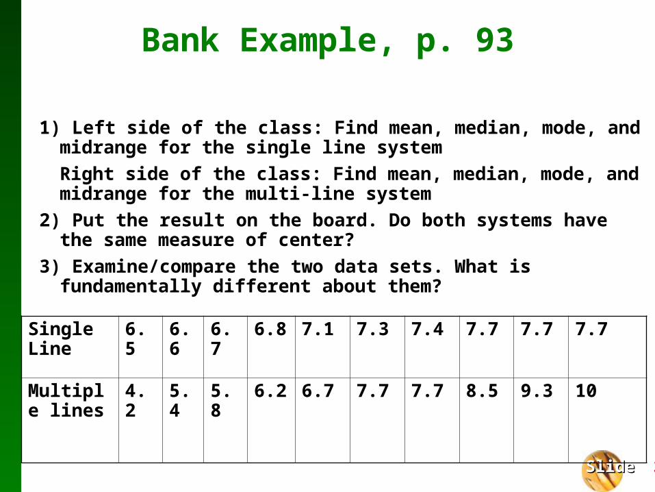
Bank Example, p. 93

1) Left side of the class: Find mean, median, mode, and midrange for the single line system

Right side of the class: Find mean, median, mode, and midrange for the multi-line system

2) Put the result on the board. Do both systems have the same measure of center?

3) Examine/compare the two data sets. What is fundamentally different about them?

Single Line

6.5 6.6 6.7 6.8 7.1 7.3 7.4 7.7 7.7 7.7

Multiple lines

4.2 5.4 5.8 6.2 6.7 7.7 7.7 8.5 9.3 10

SlideSlide 4

Definition

The range of a set of data is the difference between the maximum value and the minimum value.

Range = (maximum value) – (minimum value)

Bank 1: Variable waiting lines 6 6 6Bank 2: Single waiting lines 4 7 7

Bank 3: Multiple waiting lines 1 3 14

SlideSlide 5

Definition

The standard deviation of a set of sample values is a measure of variation of values about the mean.

If the values are close together: small s

If the values are far apart: large s.

SlideSlide 6

Sample Standard Deviation Formula (3-4)

(x - x)2

n - 1s =

SlideSlide 7

Sample Standard Deviation (Shortcut Formula: 3-5)

n (n - 1)

s =nx2) - (x)2

SlideSlide 8

Banking Example

Jefferson Valley (single line):

6.5 6.6 6.7 6.8 7.1 7.3 7.4 7.7 7.77.7

Providence (multiple lines):

4.2 5.4 5.8 6.2 6.7 7.7 7.7 8.5 9.310.0

SlideSlide 9

Using the formula for standard deviation (TI83)

1) Put stuff in L1, L2. Do 2 variable stats. The mean for L1 is ____. Find the deviation of each value from the mean. (L3: L1-___).

2) Show that the sum of deviations from Step 1 is 0. Will it always be 0? (sum L3)

3) We want to avoid the canceling out of the positive and negative deviations – so we square the deviations (L4: L3^2)

4) We need a mean of those squared deviations, so we find the mean by dividing by n-1 (degrees of freedom). (sum L4/(n-1))

5) Track the units. If the original times are in minutes, the deviations are in minutes, the squared deviations are in minutes squared (what?), and the mean is in minutes squared (huh?)

6) Since minutes squared doesn’t make much sense, take the square root to get back to the original units. (sqr rt of ans).

SlideSlide 10

Example

1) Use the data set (1, 3, 14) from the single line system to find s using formula 3-5.

2) YOU: Use the data set (4, 7, 7 minutes) from a multiple line system to find s using formula 3-5.

3) Which standard deviation is smaller? So which line is better?

SlideSlide 11

Standard Deviation - Important Properties

The standard deviation is a measure of variation of all values from the mean.

The value of the standard deviation s is usually positive.

The value of the standard deviation s can increase dramatically with the inclusion of one or more outliers (data values far away from all others).

The units of the standard deviation s are the same as the units of the original data values.

SlideSlide 12

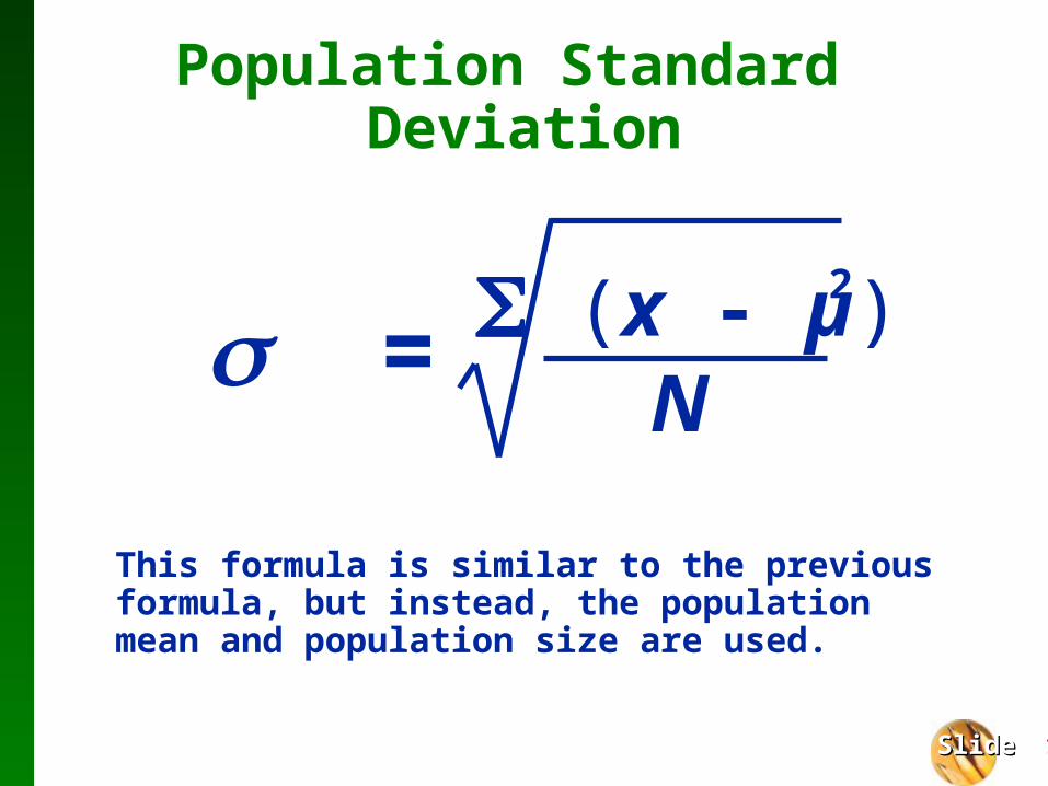
Population Standard Deviation

2 (x - µ)

N =

This formula is similar to the previous formula, but instead, the population mean and population size are used.

SlideSlide 13

Population variance: Square of the population standard deviation

Definition The variance of a set of values is a measure of

variation equal to the square of the standard deviation.

(A general description of the amount that values vary among themselves)

Also: dispersion/spread

Sample variance: Square of the sample standard deviation s

SlideSlide 14

Variance - Notation

standard deviation squared

s

2

2

}Notation

Sample variance

Population variance

SlideSlide 15

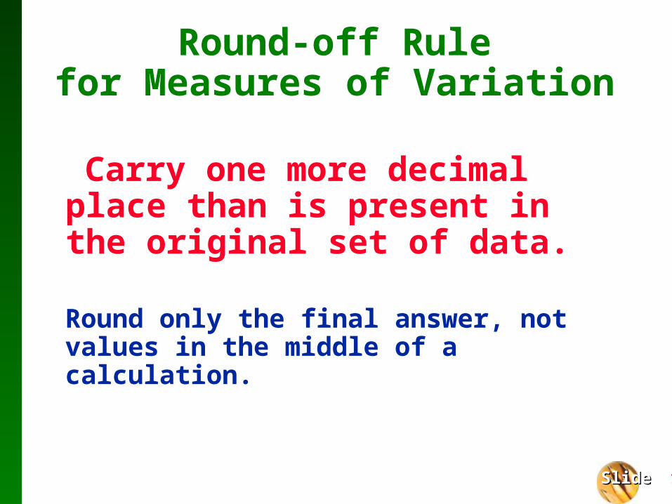
Round-off Rulefor Measures of Variation

Carry one more decimal place than is present in the original set of data.

Round only the final answer, not values in the middle of a calculation.

SlideSlide 16

Day 2 Warm Up:Heart Rate Activity

Is there a difference between male and female heart rates?

Male: 60 67 59 64 80 55 72 84 59 67 69 65 66

88 56 82 55 72 64 66 58 70 60 80 63 66 85 66 71 64

Female: 83 56 57 63 60 69 70 86 70 57 67 75 72 75 57 76 69 79 84 75 56 72 70 62 67 66 60 74 81 60

Compare the range, standard deviation, and variances of these samples.

SlideSlide 17

Estimation of Standard DeviationRange Rule of Thumb

For estimating a value of the standard deviation s,

Use

Where range = (maximum value) – (minimum value)

CRUDE estimate

Based on the principal: For many data sets, the vast majority (95%) lie within 2 std. dev.’s of the mean

Simple rule to help us interpret std. devs.

Range

4s

SlideSlide 18

Age of Best Actresses

• Use the range rule of thumb to find a rough estimate of the standard deviation of the sample of 76 ages of actresses who won Oscars.

• Max age: 80

• Min age: 21

SlideSlide 19

Estimation of Standard DeviationRange Rule of Thumb

For interpreting a known value of the standard deviation s, find rough estimates of the minimum and maximum “usual” sample values by using:

Minimum “usual” value (mean) – 2 X (standard deviation) =

Maximum “usual” value (mean) + 2 X (standard deviation) =

SlideSlide 20

Example

A statistics professor finds the times (in seconds) required to complete a quiz have a mean of 180 sec and a standard deviation of 30 secs. Is a time of 90 secs unusual? Why or why not?

YOU: Typical IQ tests have a mean of 100 and a standard deviation of 15. Use the range rule of thumb to find the usual IQ scores. Is a value of 140 unusual?

SlideSlide 21

Definition

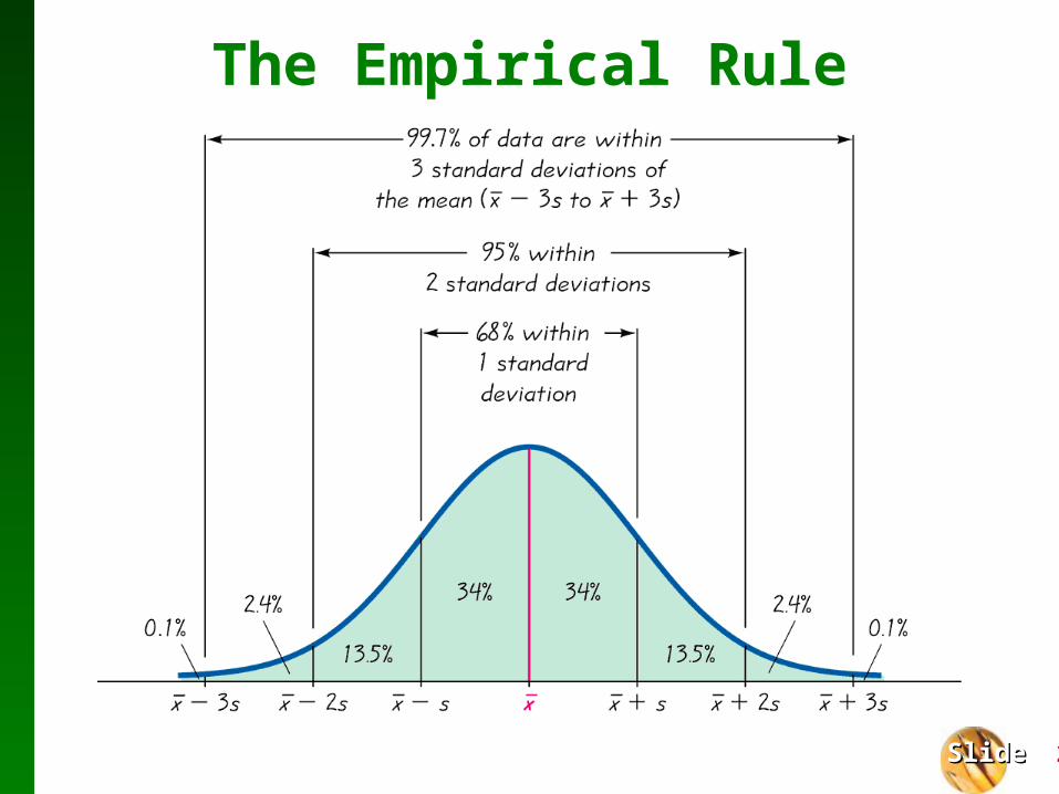
Empirical (68-95-99.7) Rule

For data sets having a distribution that is approximately bell shaped, the following properties apply:

About 68% of all values fall within 1 standard deviation of the mean.

About 95% of all values fall within 2 standard deviations of the mean.

About 99.7% of all values fall within 3 standard deviations of the mean.

SlideSlide 22

The Empirical Rule

SlideSlide 23

The Empirical Rule(applies only to bell-shaped distributions)

SlideSlide 24

The Empirical Rule

SlideSlide 25

Example: IQ Scores

• IQ scores are bell shaped with a mean of 100 and a standard deviation of 15. What percent of IQ scores fall between 70 and 130?

SlideSlide 26

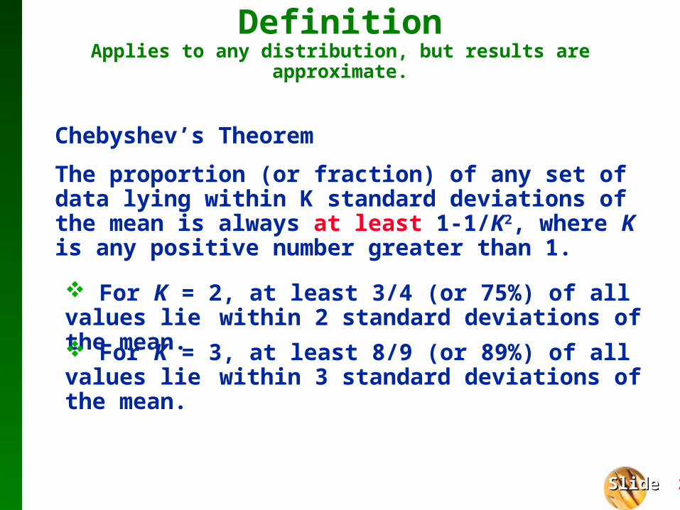
DefinitionApplies to any distribution, but results are approximate.

Chebyshev’s Theorem

The proportion (or fraction) of any set of data lying within K standard deviations of the mean is always at least 1-1/K2, where K is any positive number greater than 1.

For K = 2, at least 3/4 (or 75%) of all values lie within 2 standard deviations of the mean.

For K = 3, at least 8/9 (or 89%) of all values lie within 3 standard deviations of the mean.

SlideSlide 27

Example

• IQ scores have a mean of 100 and a standard deviation of 15 (pretend we don’t know that IQ scores are bell-shaped).

• According to Chebyshev’s Theorem, what can we conclude about:

1) 75% of the IQ scores?

2) 89% of the IQ scores?

SlideSlide 28

Rationale for using n-1 versus n

The end of Section 3-3 has a detailed explanation of why n – 1 rather than n is used. The student should study it carefully.

SlideSlide 29

Definition

The coefficient of variation (or CV) for a set of sample or population data, expressed as a percent, describes the standard deviation relative to the mean.

Free of specific units of measure

For comparing variation for values taken from different populations

SamplePopulation

sxCV = 100% CV =

100%

SlideSlide 30

Example: StatdiskHeight and Weight data for the 40 males

Data Set 1, Appendix B

• Although the difference in units makes it impossible to compare the two standard deviations (inches vs. pounds), we can compare CV’s (which have no units).

• Find the CV for weights and the CV for heights.