slide 1 of 11 fundamental theorem of calculus - confex€¦ · slide 1 of 11 fundamental theorem of...
TRANSCRIPT
Slide 1 of 11
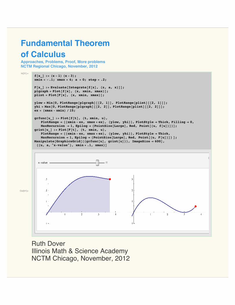
Fundamental Theoremof CalculusApproaches, Problems, Proof, More problemsNCTM Regional Chicago, November, 2012In[31]:=
f@x_D := Hx - 1L Hx - 3L;xmin = -.1; xmax = 4; a = 0; step = .2;
F@x_D := Evaluate@Integrate@f@zD, 8z, a, x<DD;plgraph = Plot@f@xD, 8x, xmin, xmax<D;plint = Plot@F@xD, 8x, xmin, xmax<D;
ylow = Min@0, PlotRange@plgraphD@@2, 1DD, PlotRange@plintD@@2, 1DDD;yhi = Max@0, PlotRange@plgraphD@@2, 2DD, PlotRange@plintD@@2, 2DDD;ex = Hxmax - xminL ê 15;
grfunc@u_D := Plot@f@tD, 8t, xmin, u<,PlotRange Ø 88xmin - ex, xmax + ex<, 8ylow, yhi<<, PlotStyle Ø Thick, Filling Ø 0,MaxRecursion Ø 1, Epilog Ø 8PointSize@LargeD, Red, Point@8u, f@uD<D<D;
grint@u_D := Plot@F@tD, 8t, xmin, u<,PlotRange Ø 88xmin - ex, xmax + ex<, 8ylow, yhi<<, PlotStyle Ø Thick,MaxRecursion Ø 1, Epilog Ø 8PointSize@LargeD, Red, Point@8u, F@uD<D< D;
Manipulate@GraphicsGrid@88grfunc@uD, grint@uD<<, ImageSize Ø 600D,88u, a, "x-value"<, xmin + .1, xmax<D
Out[41]=
x-value
Ruth DoverIllinois Math & Science AcademyNCTM Chicago, November, 2012

Slide 2 of 11
WHY give a talk on the FTC?
Ï Mean scores on many AP exam problems are disappointingly low.
Recent Examples 2012 AB/BC 3 Means: AB: 2.67 BC: 4.29
2011 AB/BC 4 Means: AB: 2.44 BC: 3.84
Ï Most major textbooks contain very few problems similar to these.But you can write problems!
Ï Let’s see... Take one function, use it to create another function... This is very difficult for many students.
2 NCTMChicago2012FTC.nb

Slide 3 of 11
Notes
® Order of topics: Riemann sums, FTC’s, properties of integralsChoose any permutation you’d like.
© Use technology! Calculators or computers.
™ Antiderivatives. Early or late. For today, I’ll assume this.
´ Notation: I’ll assume the understanding of Ÿaxƒ HtL „t as representing signed area.
Today: A short, quick version!
NCTMChicago2012FTC.nb 3

Slide 4 of 11
Distance traveled
If a car travels at 45 mph for a total of 3 hours, then the distance traveled is simply rate · time = 45 · 3 = 135miles. This result may be represented by the area under the velocity function.
In[42]:=Plot@45, 8t, 0, 3<, Filling Ø Axis, PlotRange Ø 80, 50<,Ticks Ø 8Automatic, 845<<, PlotLabel Ø "Area = 135"D
Out[42]=
If the velocity is a linear function, say v = 20t, the distance traveled may also be calculated.
In[43]:=Plot@20 t, 8t, 0, 3<, Filling Ø Axis, PlotLabel Ø "Area = 90"D
Out[43]=
What if we go forward for a while and then backwards, both at constant speeds?(Please ignore reality for a little while here!)This is the total signed area.
4 NCTMChicago2012FTC.nb

In[44]:=PlotB ¶
30 0 § t < 2-10 2 § t < 3
, 8t, 0, 3<, Filling Ø Axis,
Ticks Ø 8Automatic, 8-10, 30<<, PlotLabel -> "Displacement = 60 - 10 = 50"F
Out[44]=
NCTMChicago2012FTC.nb 5
Slide 5 of 11
Accumulation -Distance at time t
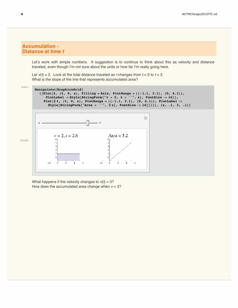
Let’s work with simple numbers. A suggestion is to continue to think about this as velocity and distancetraveled, even though I’m not sure about the units or how far I’m really going here.
Let v(t) = 2. Look at the total distance traveled as t changes from t = 0 to t = 3.What is the slope of the line that represents accumulated area?
In[45]:=Manipulate@GraphicsGrid@
88Plot@2, 8t, 0, x<, Filling Ø Axis, PlotRange Ø 88-1.1, 3.1<, 80, 6.1<<,PlotLabel Ø Style@StringForm@"v = 2, t = ``", xD, FontSize -> 16DD,
Plot@2 t, 8t, 0, x<, PlotRange Ø 88-1.1, 3.1<, 80, 6.1<<, PlotLabel ->Style@StringForm@"Area = ``", 2 xD, FontSize -> 16DD<<D, 8x, .1, 3, .1<D
Out[45]=
x
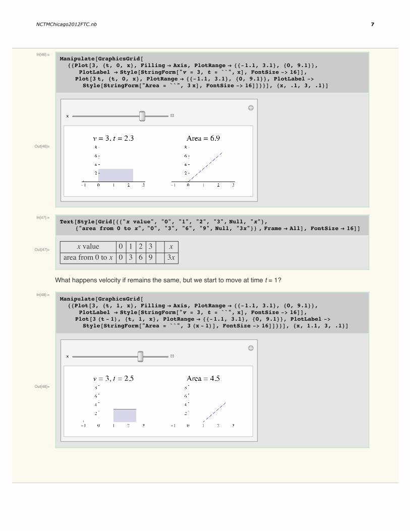
What happens if the velocity changes to v(t) = 3?How does the accumulated area change when v = 3?
6 NCTMChicago2012FTC.nb
In[46]:=Manipulate@GraphicsGrid@
88Plot@3, 8t, 0, x<, Filling Ø Axis, PlotRange Ø 88-1.1, 3.1<, 80, 9.1<<,PlotLabel Ø Style@StringForm@"v = 3, t = ``", xD, FontSize -> 16DD,
Plot@3 t, 8t, 0, x<, PlotRange Ø 88-1.1, 3.1<, 80, 9.1<<, PlotLabel ->Style@StringForm@"Area = ``", 3 xD, FontSize -> 16DD<<D, 8x, .1, 3, .1<D
Out[46]=
x
In[47]:=Text@Style@Grid@88"x value", "0", "1", "2", "3", Null, "x"<,
8"area from 0 to x", "0", "3", "6", "9", Null, "3x"<< , Frame Ø AllD, FontSize Ø 16DD
Out[47]= x value 0 1 2 3 xarea from 0 to x 0 3 6 9 3x
What happens velocity if remains the same, but we start to move at time t = 1?
In[48]:=Manipulate@GraphicsGrid@
88Plot@3, 8t, 1, x<, Filling Ø Axis, PlotRange Ø 88-1.1, 3.1<, 80, 9.1<<,PlotLabel Ø Style@StringForm@"v = 3, t = ``", xD, FontSize -> 16DD,
Plot@3 Ht - 1L, 8t, 1, x<, PlotRange Ø 88-1.1, 3.1<, 80, 9.1<<, PlotLabel ->Style@StringForm@"Area = ``", 3 Hx - 1LD, FontSize -> 16DD<<D, 8x, 1.1, 3, .1<D
Out[48]=
x
NCTMChicago2012FTC.nb 7
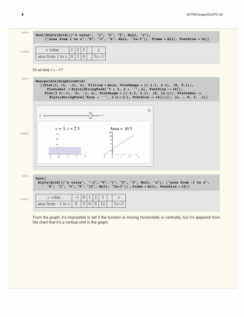
In[49]:=Text@Style@Grid@88"x value", "1", "2", "3", Null, "x"<,
8"area from 1 to x", "0", "3", "6", Null, "3x-3"<< , Frame Ø AllD, FontSize Ø 16DD
Out[49]= x value 1 2 3 xarea from 1 to x 0 3 6 3x-3
Or at time t = –1?
In[50]:=Manipulate@GraphicsGrid@
88Plot@3, 8t, -11, x<, Filling Ø Axis, PlotRange Ø 88-1.1, 3.1<, 80, 9.1<<,PlotLabel Ø Style@StringForm@"v = 3, t = ``", xD, FontSize -> 16DD,
Plot@3 Ht + 1L, 8t, -1, x<, PlotRange Ø 88-1.1, 3.1<, 80, 12.1<<, PlotLabel ->Style@StringForm@"Area = ``", 3 Hx + 1LD, FontSize -> 16DD<<D, 8x, -.9, 3, .1<D
Out[50]=
x
In[51]:=Text@Style@Grid@88"x value", "-1", "0", "1", "2", "3", Null, "x"<, 8"area from -1 to x",
"0", "3", "6", "9", "12", Null, "3x+3"<< , Frame Ø AllD, FontSize Ø 16DD
Out[51]= x value -1 0 1 2 3 xarea from -1 to x 0 3 6 9 12 3x+3
From the graph, it’s impossible to tell if the function is moving horizontally or vertically, but it’s apparent fromthe chart that it’s a vertical shift in the graph.
8 NCTMChicago2012FTC.nb
Slide 6 of 11
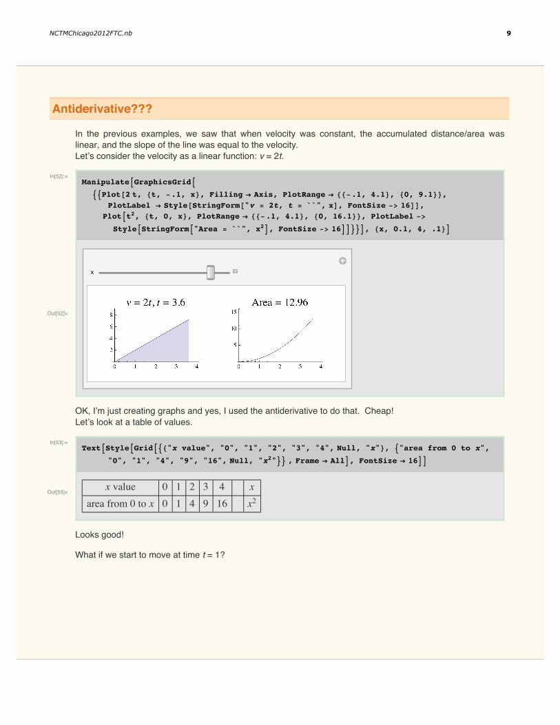
Antiderivative???
In the previous examples, we saw that when velocity was constant, the accumulated distance/area waslinear, and the slope of the line was equal to the velocity.Let’s consider the velocity as a linear function: v = 2t.
In[52]:=ManipulateAGraphicsGridA
99Plot@2 t, 8t, -.1, x<, Filling Ø Axis, PlotRange Ø 88-.1, 4.1<, 80, 9.1<<,PlotLabel Ø Style@StringForm@"v = 2t, t = ``", xD, FontSize -> 16DD,
PlotAt2, 8t, 0, x<, PlotRange Ø 88-.1, 4.1<, 80, 16.1<<, PlotLabel ->
StyleAStringFormA"Area = ``", x2E, FontSize -> 16EE==E, 8x, 0.1, 4, .1<E
Out[52]=
x
OK, I’m just creating graphs and yes, I used the antiderivative to do that. Cheap!Let’s look at a table of values.
In[53]:=TextAStyleAGridA98"x value", "0", "1", "2", "3", "4", Null, "x"<, 9"area from 0 to x",
"0", "1", "4", "9", "16", Null, "x2"== , Frame Ø AllE, FontSize Ø 16EE
Out[53]=x value 0 1 2 3 4 x
area from 0 to x 0 1 4 9 16 x2
Looks good!
What if we start to move at time t = 1?
NCTMChicago2012FTC.nb 9

In[54]:=ManipulateAGraphicsGridA
99Plot@2 t, 8t, 1, x<, Filling Ø Axis, PlotRange Ø 88-.1, 4.1<, 80, 9.1<<,PlotLabel Ø Style@StringForm@"v = 2t, t = ``", xD, FontSize -> 16DD,
PlotAt2 - 1, 8t, 1 , x<, PlotRange Ø 88-.1, 4.1<, 80, 16.1<<, PlotLabel ->
StyleAStringFormA"Area = ``", x2 - 1E, FontSize -> 16EE==E, 8x, 1.1, 4, .1<E
Out[54]=
x
In[55]:=TextA
StyleAGridA98"x value", "1", "2", "3", "4", Null, "x"<, 9"area from 0 to x", "0",
"3", "8", "9", Null, "x2-1"== , Frame Ø AllE, FontSize Ø 16EE
Out[55]=x value 1 2 3 4 x
area from 0 to x 0 3 8 9 x2-1
Or if we start at t = -1? Note that this introduces a section with v < 0.
10 NCTMChicago2012FTC.nb

In[56]:=ManipulateAGraphicsGridA
99Plot@2 t, 8t, -1, x<, Filling Ø Axis, PlotRange Ø 88-1.1, 3.1<, 8-2.1, 6.1<<,PlotLabel Ø Style@StringForm@"v = 2t, t = ``", xD, FontSize -> 16DD,
PlotAt2 - 1, 8t, -1 , x<, PlotRange Ø 88-1.1, 3.1<, 8-2.1, 9.1<<, PlotLabel ->
StyleAStringFormA"Area = ``", x2 - 1E, FontSize -> 16EE==E, 8x, -.9, 3, .1<E
Out[56]=
x
In[57]:=TextA
StyleAGridA98"x value", "-1", "0", "1", "2", "3", Null, "x"<, 9"area from 0 to x",
"0", "-1", "0", "3", "8", Null, "x2-1"== , Frame Ø AllE, FontSize Ø 16EE
Out[57]=x value -1 0 1 2 3 x
area from 0 to x 0 -1 0 3 8 x2-1
Or if we start at t = -2?
NCTMChicago2012FTC.nb 11
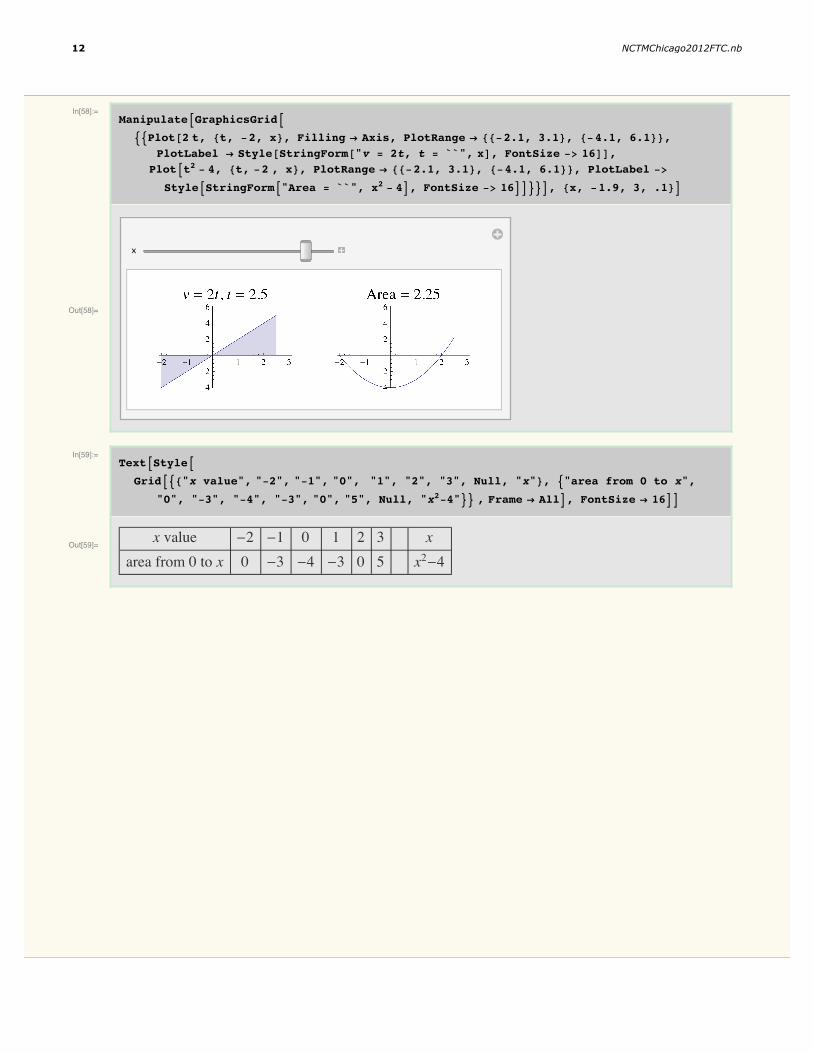
In[58]:=ManipulateAGraphicsGridA
99Plot@2 t, 8t, -2, x<, Filling Ø Axis, PlotRange Ø 88-2.1, 3.1<, 8-4.1, 6.1<<,PlotLabel Ø Style@StringForm@"v = 2t, t = ``", xD, FontSize -> 16DD,
PlotAt2 - 4, 8t, -2 , x<, PlotRange Ø 88-2.1, 3.1<, 8-4.1, 6.1<<, PlotLabel ->
StyleAStringFormA"Area = ``", x2 - 4E, FontSize -> 16EE==E, 8x, -1.9, 3, .1<E
Out[58]=
x
In[59]:=TextAStyleA
GridA98"x value", "-2", "-1", "0", "1", "2", "3", Null, "x"<, 9"area from 0 to x",
"0", "-3", "-4", "-3", "0", "5", Null, "x2-4"== , Frame Ø AllE, FontSize Ø 16EE
Out[59]=x value -2 -1 0 1 2 3 x
area from 0 to x 0 -3 -4 -3 0 5 x2-4
12 NCTMChicago2012FTC.nb

Slide 7 of 11
More interesting?
Back to the original picture:
In[60]:=f@x_D := Hx - 1L Hx - 3L;xmin = -.1; xmax = 4; a = 0; step = .2;
F@x_D := Evaluate@Integrate@f@zD, 8z, a, x<DD;plgraph = Plot@f@xD, 8x, xmin, xmax<D;plint = Plot@F@xD, 8x, xmin, xmax<D;
ylow = Min@0, PlotRange@plgraphD@@2, 1DD, PlotRange@plintD@@2, 1DDD;yhi = Max@0, PlotRange@plgraphD@@2, 2DD, PlotRange@plintD@@2, 2DDD;ex = Hxmax - xminL ê 15;
grfunc@u_D := Plot@f@tD, 8t, xmin, u<,PlotRange Ø 88xmin - ex, xmax + ex<, 8ylow, yhi<<, PlotStyle Ø Thick, Filling Ø 0,MaxRecursion Ø 1, Epilog Ø 8PointSize@LargeD, Red, Point@8u, f@uD<D<D;
grint@u_D := Plot@F@tD, 8t, xmin, u<,PlotRange Ø 88xmin - ex, xmax + ex<, 8ylow, yhi<<, PlotStyle Ø Thick,MaxRecursion Ø 1, Epilog Ø 8PointSize@LargeD, Red, Point@8u, F@uD<D< D;
Manipulate@GraphicsGrid@88grfunc@uD, grint@uD<<, ImageSize Ø 600D,88u, a, "x-value"<, xmin + .1, xmax<D
Out[70]=
x-value
Change the starting value - the lower limit of integration.
NCTMChicago2012FTC.nb 13
Slide 8 of 11
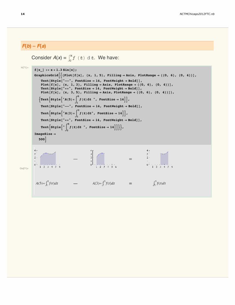
F(b) – F(a)
Consider A(x) = Ÿcxƒ HtL „t. We have:
In[71]:=f@x_D := x + 1.3 Sin@xD;
GraphicsGridB:8Plot@f@xD, 8x, 1, 5<, Filling Ø Axis, PlotRange Ø 880, 6<, 80, 4<<D,
Text@Style@"––", FontSize Ø 14, FontWeight Ø BoldDD,Plot@f@xD, 8x, 1, 3<, Filling Ø Axis, PlotRange Ø 880, 6<, 80, 4<<D,Text@Style@"==", FontSize Ø 14, FontWeight Ø BoldDD,Plot@f@xD, 8x, 3, 5<, Filling Ø Axis, PlotRange Ø 880, 6<, 80, 4<<D<,
:TextBStyleB"AH5L=‡1
5ƒHtL„t ", FontSize Ø 14FF,
Text@Style@"––", FontSize Ø 14, FontWeight Ø BoldDD,
TextBStyleB"AH3L=‡1
3ƒHtL„t", FontSize Ø 14FF,
Text@Style@"==", FontSize Ø 14, FontWeight Ø BoldDD,
TextBStyleB"‡3
5ƒHtL„t ", FontSize Ø 14FF>>,
ImageSize Ø
500F
Out[71]=
14 NCTMChicago2012FTC.nb
Slide 9 of 11
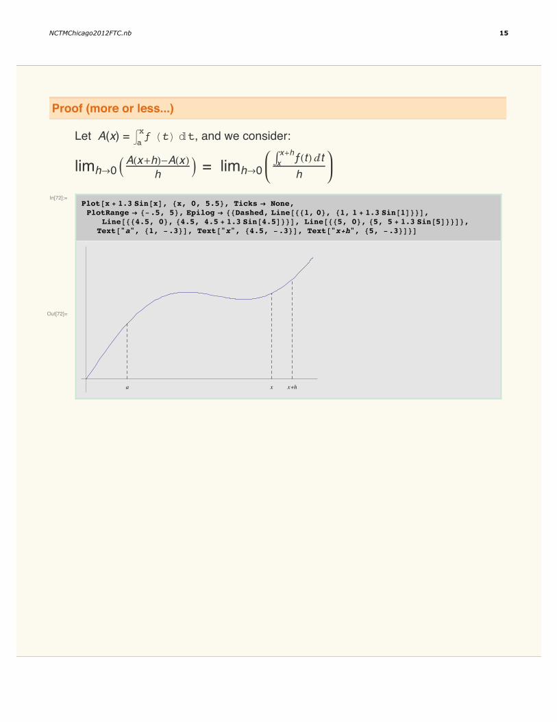
Proof (more or less...)
Let A(x) = Ÿaxƒ HtL „t, and we consider:
limhØ0 IAHx+hL-AHxL
h M = limhØ0Ÿxx+hƒHtL „t
h
In[72]:=Plot@x + 1.3 Sin@xD, 8x, 0, 5.5<, Ticks Ø None,PlotRange Ø 8-.5, 5<, Epilog Ø 88Dashed, Line@881, 0<, 81, 1 + 1.3 Sin@1D<<D,
[email protected], 0<, 84.5, 4.5 + 1.3 [email protected]<<D, Line@885, 0<, 85, 5 + 1.3 Sin@5D<<D<,Text@"a", 81, -.3<D, Text@"x", 84.5, -.3<D, Text@"x+h", 85, -.3<D<D
Out[72]=
a x x+h
NCTMChicago2012FTC.nb 15
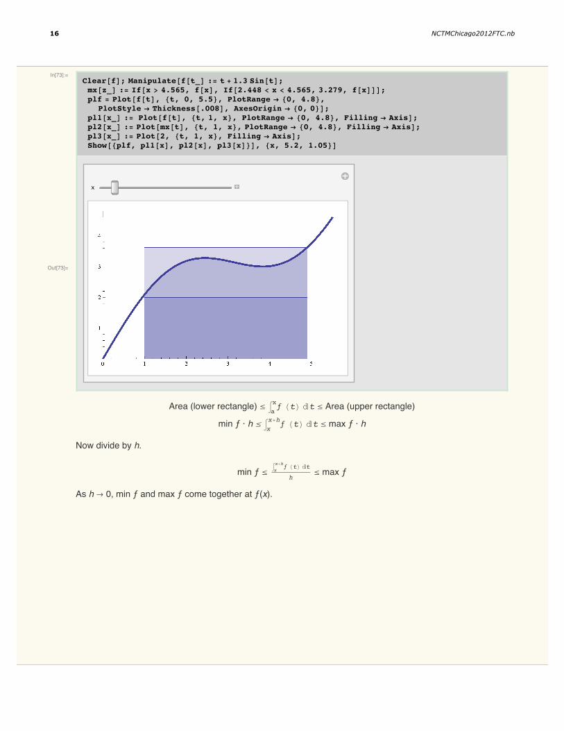
In[73]:=Clear@fD; Manipulate@f@t_D := t + 1.3 Sin@tD;mx@z_D := If@x > 4.565, f@xD, [email protected] < x < 4.565, 3.279, f@xDDD;plf = Plot@f@tD, 8t, 0, 5.5<, PlotRange Ø 80, 4.8<,
PlotStyle Ø [email protected], AxesOrigin Ø 80, 0<D;pl1@x_D := Plot@f@tD, 8t, 1, x<, PlotRange Ø 80, 4.8<, Filling Ø AxisD;pl2@x_D := Plot@mx@tD, 8t, 1, x<, PlotRange Ø 80, 4.8<, Filling Ø AxisD;pl3@x_D := Plot@2, 8t, 1, x<, Filling Ø AxisD;Show@8plf, pl1@xD, pl2@xD, pl3@xD<D, 8x, 5.2, 1.05<D
Out[73]=
x
Area (lower rectangle) § Ÿaxƒ HtL „t § Area (upper rectangle)
min ƒ · h § Ÿxx+hƒ HtL „t § max ƒ · h
Now divide by h.
min ƒ § Ÿxx+hƒ HtL „t
h § max ƒ
As h Ø 0, min ƒ and max ƒ come together at ƒ(x).
16 NCTMChicago2012FTC.nb
Slide 10 of 11
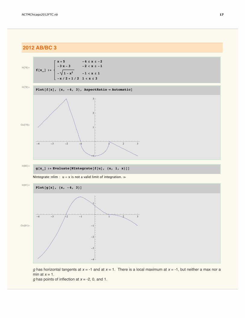
2012 AB/BC 3
In[78]:=f@x_D :=
x + 5 -4 § x § -2-3 x - 3 -2 < x § -1
- 1 - x2 -1 < x § 1-x ê 2 + 1 ê 2 1 < x § 3
In[79]:=Plot@f@xD, 8x, -4, 3<, AspectRatio Ø AutomaticD
Out[79]=
-4 -3 -2 -1 1 2 3
-1
1
2
3
In[80]:=g@x_D := Evaluate@NIntegrate@f@uD, 8u, 1, x<DD
NIntegrate::nlim : u = x is not a valid limit of integration. à
In[81]:=Plot@g@xD, 8x, -4, 3<D
Out[81]=
-4 -3 -2 -1 1 2 3
-4
-3
-2
-1
1
g has horizontal tangents at x = -1 and at x = 1. There is a local maximum at x = -1, but neither a max nor amin at x = 1.g has points of inflection at x = -2, 0, and 1.
NCTMChicago2012FTC.nb 17
Slide 11 of 11
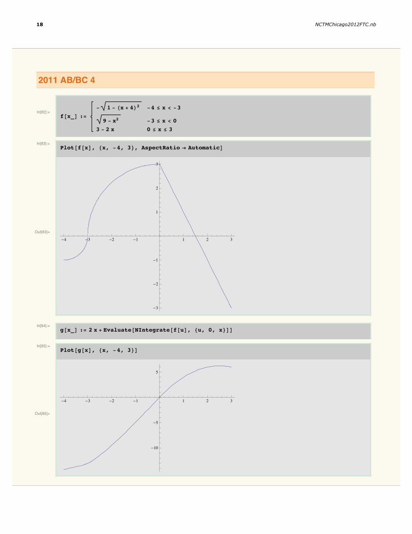
2011 AB/BC 4
In[82]:=f@x_D :=
- 1 - Hx + 4L2 -4 § x < -3
9 - x2 -3 § x < 03 - 2 x 0 § x § 3
In[83]:=Plot@f@xD, 8x, -4, 3<, AspectRatio Ø AutomaticD
Out[83]=
-4 -3 -2 -1 1 2 3
-3
-2
-1
1
2
3
In[84]:=g@x_D := 2 x + Evaluate@NIntegrate@f@uD, 8u, 0, x<DD
In[85]:=Plot@g@xD, 8x, -4, 3<D
Out[85]=
-4 -3 -2 -1 1 2 3
-10
-5
5
18 NCTMChicago2012FTC.nb

g has an absolute maximum at x = 5/2 since g’(x) = 2 + ƒ(x) = 0 and g’ changes from positive to negative atx = 5/2.
g has points of inflection at x = 0 since ƒ changes from increasing to decreasing at x = 0.
NCTMChicago2012FTC.nb 19