size rationalization and trade exposure in developing

This PDF is a selection from an out-of-print volume from the National Bureauof Economic Research

Volume Title: Empirical Studies of Commercial Policy

Volume Author/Editor: Robert E. Baldwin, editor

Volume Publisher: University of Chicago Press, 1991

Volume ISBN: 0-226-03569-7

Volume URL: http://www.nber.org/books/bald91-1

Conference Date: March 16-17, 1990

Publication Date: January 1991

Chapter Title: Size Rationalization and Trade Exposure in Developing Countries

Chapter Author: Mark J. Roberts, James R. Tybout

Chapter URL: http://www.nber.org/chapters/c6713

Chapter pages in book: (p. 169 - 200)

6 Size Rationalization and Trade Exposure in Developing Countries Mark J. Roberts and James R. Tybout

6.1 Overview

Economists often argue that exposure to foreign competition should increase plant size and productivity in less developed countries (LDCs). They cite several reasons. First, foreign competition reduces the market power that domestic producers may derive from scale economies, rationed credit markets, or institutional constraints. Consequently, reductions in protection should expand output among these producers and allow better exploitation of scale economies. Similarly, when competitive discipline is absent, the resultant cushion of monopoly profits may allow inefficiently small, wasteful domestic firms to survive. Finally, even if profits are competed away through entry or the threat of entry, limited domestic demand can lead to inefficiently small-scale production in markets for differentiated products, where Cham- berlinian competition prevails.

These positive effects of trade exposure are widely held to apply both in developing and in industrialized economies. Nonetheless, analytical models show that they need not obtain. Whether trade liberalization improves efficiency depends critically on the distribution of output adjustments across plants with differing unit costs (Rodrik 1988a). This depends, in turn, on factor intensities, the pattern of demand shifts, the nature of competition, and the extent to which entry and exit are possible (e.g., Buffie and Spiller 1986;

Mark 1. Roberts is professor of economics at the Pennsylvania State University. James R. Ty- bout is associate professor of economics at Georgetown University and a consultant to the World Bank.

Funding was provided by the NBER and the World Bank research project “Industrial Competi- tion, Productive Efficiency, and Their Relation to Trade Regimes” (RPO-674-46). We have ben- efited from the comments of Robert Baldwin, Ann Harrison, Anne Krueger, Robert Lipsey, Ra- mon Lopez, Peter Petri, Larry Samuelson, and Marius Schwartz. We also wish to thank Constantina Backinezos, Jin-Sung Park, and Lili Liu for research assistance.

169

170 Mark J. Roberts and James R. Qbout

Brown, 1989). When technology and innovation are endogenous, further am- biguities result (Rodrik 1988b).

Simulation models support the received wisdom that in LDCs, liberalization of imperfectly competitive industries results in larger plants and higher efficiency (Condon and de Melo 1986; Devarajan and Rodrik 1989a, 1989b; de Melo and Roland-Holst, chap. 10 in this volume). Disturbingly, however, there is very little micro-econometric evidence confirming the adjustment mechanisms that these models assume. For example, Bhagwati (1988) con- cludes: “Although the arguments for the success of the [outward-oriented development strategies] based on economies of scale and X-efficiency are plausible, empirical support for them is not available.” Pack (1989) goes further, claiming that the link between trade liberalization and productivity growth has not been established at all.’

Given the lack of direct evidence regarding industrial adjustment in response to trade liberalization, this paper tackles a very basic question. Specif- ically, in LDCs, how is trade orientation correlated with the size distribution of plants and with plant-level labor productivity? We begin with a simple model that summarizes some effects of trade exposure on producer size and productive efficiency that have been stressed in the recent analytical and simulation literature. We then examine annual plant-level data from Chile and Colombia to determine whether these effects can be confirmed.

The empirical results indicate that, over the long run, higher trade exposure is correlated with smaller plant sizes, controlling for industry and country effects. However, the mix of high versus low productivity plants is not strongly associated with trade exposure. Both of these findings cast doubt on the mechanisms linking trade, plant size, and productivity in a number of recent analytical and simulation studies.

6.2 Theories Linking ’hade Regime and Size Rationalization

6.2.1 The Analytics of Size Rationalization under Imperfect Competition

To motivate our empirical work, we begin with an expository model that generates several predictions familiar from the trade and development literature.2 First, assume that within each industry, domestically produced goods

1. Pack (1989) writes: “Comparisons of total factor productivity growth among countries pur- suing different international trade orientations do not reveal systematic differences in productivity growth in manufacturing, nor do the time-series studies of individual countries that have experi- enced alternating trade regimes allow strong conclusions in this dimension. . . . Moreover, the firm-level data collected for estimation of production frontiers are quite reliable and confirm the pattern established at more aggregated levels.”

2. Buffie and Spiller (1986), Dixit and Norman (1980), Dutz (1990), Lancaster (1984). Help- man and Krugman (1985), Horstmann and Markusen (l986), and Markusen (1981) are among the many relevant references in the analytical literature. Simulation results that reflect at least some of the effects described here include those found in Harris (1984). Rodrik (1988a), Devarajan and

171 Size Rationalization and Trade Exposure

are perfect substitutes, and domestic firms are Cournot quantity competitors vis-2-vis one another. Also, let the domestic product be an imperfect substitute for imports, so that the demand curve faced by domestic producers may be written as P = P ( Q , n ) , where Q = Zq,, q, is the output of the irh producer, and R is the set of factors that determine exposure to world rnarket~.~ This set includes quantitative restrains (QRs), tariffs, and the real exchange rate. Fi- nally, define C, = F + q,c, to be the total costs of producing q, borne by the irh plant (i = 1, n), where F and c, are constants. The presence of marginal cost heterogeneity is meant to reflect differences in managerial abilities, credit market access, and capital s t o ~ k s . ~

As is well known, the first-order condition for profit maximization under Cournot competition is

so firms with low marginal costs are relatively large.5 Also, summing equation (1) over all plants, equilibrium output and price in this market depend only on the sum of marginal costs and not on the distribution of marginal costs across plants (e.g., Bergstrom and Varian 1985):

n

nP ( Q J U + QPJQAN = 2 c,. , = I

(2)

Given n, and assuming P, < 0, there is thus a negative monotonic relationship between Zc, and the equilibrium industry output, Q. In turn, given Q , each plant’s output q, is determined recursively by equation (1).

If market entry and exit are free, the number of firms is endogenous. To characterize equilibrium in this case, we require that the last and least efficient plant (plant n) covers costs, and that all potential firms not in the market antic- ipate losses upon entry. Sorting plants in order of increasing average cost, this condition amounts to

( 3 )

Rodrik (1989a. 1989b). Condon and de Melo (1990), de Melo and Roland-Holst (chap. 10, in this volume), and Tan and de Melo (forthcoming). If there is a novelty to our model, it is that we simultaneously treat cost heterogeneity and entryiexit effects.

3. Domestic markets are small relative to the rest of the world, and foreign producers do not react strategically to domestic producers’ behavior.

4. Most models in the trade literature do not allow for marginal cost heterogeneity; we include it here for two reasons. First, it captures the spirit of the X-efficiency arguments found in the development literature. Second, it is an important feature of theoretical models that explain the persistent size heterogeneity one finds in virtually all plant-level census data (e.g., Jovanovic 1982).

5 . We do not believe the link between size and efficiency is well established in the empirical literature on developing countries. However, as this link is assumed in most analytical and simulation models, we assume it holds here to demonstrate how these models work.

172 Mark J. Roberts and James R. ”bout

where q,+, is the output level the n + lth (potential) plant would choose if it were to enter the market.

6.2.2 Demand Shifts and Rationalization

We can now review predictions about the link between demand shifts and the size distribution of plants. Hereafter, any shift that results in plant size adjustments that reduce the industry-wide average cost will be said to have “rationalized” industry. In our framework this can occur two ways-either by increasing output levels overall and reducing average fixed costs, or by shifting market shares toward large, low marginal cost plants and reducing average variable costs.

To describe the conditions under which trade liberalization induces such shifts, it is convenient to assume a linear demand schedule with both the inter- cept and the slope dependent upon trade regime:

(4) P = 01 - PQ, O1 = O1(0), p = p(n).

Then, if entry is not possible, equilibrium is described by the follow n + 2 conditions:

(5.1)

(5.3)

ci + C C i p=- (n + 1)’ 01 + Cc, - c,(n + 1)

P(n + 1) , j = 1, n. 4, =

From these equations, the effect of demand shifts induced by trade reforms follow easily. Suppose that, beginning from autarky and binding QRs, trade is liberalized. This type of reform has the effect of placing domestic producers in large world markets where there are many other producers and substitute products. Regardless of whether the domestic product is exportable or import competing, one would expect its demand elasticity to rise. We isolate the con- sequences of such an elasticity increase by pivoting the demand curve through the pre-reform equilibrium point, reducing both ci and p. By equation (5.2) P must fall, so Q must rise, and industry-wide average fixed costs must fall. The market share of plant j , qj/Q, does not depend on p. However, reductions in 01 increase the market share of large, low-cost plants, and thereby reduce average variable costs for the industry.6 So trade reforms that increase the elasticity of demand without shifting it inward reduce average costs, both by shifting production toward low-cost producers and by increasing industry-wide output.

6. More precisely, the market share of thejth plant expands as a falls if c, is less than Ccln.


Of course elasticity effects are not the only possible effect of increased foreign competition. Trade reforms that amount to tariff reductions or real currency appreciation may act mainly to reduce domestic demand for import- competing products. If this causes a contraction in total output, average fixed costs will rise for the affected industries, at least partly offsetting any fall in average variable costs. Although many simulation models allow for this contractionary effect of liberalization, it has not usually proved to be dominant.’

Now consider the adjustments that occur when entry and exit are possible. Suppose trade liberalization shifts demand inward (reduces a), with or without an increase in elasticity. By equation (5.2), P must fall, so the smallest, least efficient firms will begin to take losses and exit, reducing both n and Z C ~ . ~ In the initial equilibrium c, 5 P (eq. [3]), so before price adjusts this exit will have reduced nP more than it reduced Zci. Accordingly, to restore equilibrium Q must contact more and P must fall less than they would have if exit were not possible (eq. [2]). In sum, compared to the case of no exit, efficiency effects are stronger for two reasons: The least efficient plants leave the market entirely, and remaining plants face less contractionary pressure. By analogous logic, free entry and exit exacerbate the reduction in productive efficiency associated with outward shifts of the demand curve, as might accompany quotas or increases in the tariff rate: Small, inefficient firms are induced to enter and take market shares from incumbents. This consequence of market expansion through protection is another familiar story in the literature.

6.2.3 Robustness

Though far from comprehensive, the exposition above gives an idea of the size rationalization effects that have recently been stressed in literature. In particular, exposure to foreign competition can increase plants’ size by increasing the elasticity of demand. Even if exposure to competition reduces plant size by contracting demand, it is likely to hit the most inefficient plants hardest. Hence, unless returns to scale are important, efficiency gains are still likely. Finally, the positive effects of liberalization are larger when entry and exit are possible because inefficient plants will be forced out of the market, allowing those producers who remain behind to operate on a larger scale.

Although these effects are often stressed, they are not guaranteed. There is no reason why liberalizations might not contract demand for domestic products so severely as to increase average costs-particularly when fixed costs and entry barriers are significant. Moreover, as various authors have shown, alternative analytic frameworks expand the range of possible outcomes. For

7. An exception is de Melo and Tarr (forthcoming). 8. To see this, note that the demand function (4) and the profit maximization condition ( 1 ) imply

9. Although their models are different, the same conclusions are stressed in Eastman and Sty- qf = ( p - cf)/p, j = I , n. If P falls, qi must fall, and so average costs at the ith plant must rise.

kolt (1966), Dixit and Norman (1980), and Harris (1984).

174 Mark J. Roberts and James R. ’Qbout

example, if static Cournot quantity competition is replaced with another type of competition, firms adjust their output levels differently in response to demand shifts. The monotonic negative relationship between plant size and average variable costs might then be broken, and it would no longer necessarily hold that shifting production toward large plants improves efficiency. Still more outcomes are possible if one endogenizes marginal costs, allowing for changes in factor prices, X-efficiency, and learning-by-doing. Finally, domestic product differentiation can be introduced. This not only opens the possibility of cross-plant variation in the degree of competition from foreign substitutes, it also allows endogenous adjustments in the length of production runs.

Given these qualifications, it is clearly an empirical question whether trade liberalization will (1) increase the average scale of production, (2) shift market shares toward large producers, and (3) bring with it productivity improve- ment. The remainder of this paper is devoted to an econometric examination of these issues.

6.3 Empirical Methodology

6.3.1 The Data and Country Backgrounds

In this section we examine cross-country and intertemporal contrasts in trade exposure, plant size distributions, and labor productivity distributions for evidence on the empirical relevance of the theoretical effects reviewed in section 6.2. To do this we utilize annual census data covering all manufacturing plants with at least ten workers in Colombia and Chile.’O But before turning to the empirical models these data support, it is useful to review the cross-country differences and within-country time series fluctuations in trade policies and industrial performance that allow us to identify parameters.

Chile

The Chilean data used in this paper cover the period 1979-85; we begin our overview with the years immediately preceding. Like much of Latin America, Chile pursued an inward-oriented development strategy in the 1960s. The system of incentives-including tariffs, quotas, exchange rate policy, and domestic market regulations-favored manufacturing at the ex- pense of agriculture and import-competing producers over exporters (Corbo 1985). This bias intensified in the early 1970s. By 1973 average tariff rates exceeded 100 percent, prior deposit requirements for importers created heavy

10. The governments of Chile and Colombia have recently made these data available to the World Bank in connection with the World Bank research project “Industrial Competition, Produc- tive Efficiency, and Their Relation to Trade Regimes” (RPO 674-46). They are described in Roberts (1989) and Tybout (1989). Our discussion of Chile is based on Tybout (1989); our discussion of Colombia is based on Roberts (1989).


additional surcharges, and a complex system of multiple exchange rates pre- vailed.

In 1973, the military seized power and began implementing radical policy changes. In addition to fiscal austerity and price stabilization programs, the new government rapidly implemented laissez-faire micro reforms. The new administration sold public enterprises, decontrolled prices and interest rates, and dismantled trade barriers. The average nominal tariff rate fell from 105 percent in 1974 to 12 percent in 1979.

Although the industrial sector initially suffered from recessionary macro conditions, recovery began in 1976 and continued into 1981. Several features of this recovery were noteworthy. First, the reductions in industrial employment that accompanied the 1974-75 recession continued during the 1976-8 1 recovery, so that labor productivity increased dramatically. Second, the bal- ance of trade in industrial products worsened considerably during the latter part of the recovery period. The trade liberalization was partly responsible, but there was also considerable exchange-rate appreciation beginning in 1979. Third, during 1976-81 a handful of powerful conglomerates (grupos) emerged and consolidated control over both financial and industrial enterprises.

By the end of 1982, the Chilean economy was again in serious trouble. The exchange rate had been overvalued for some time, and tradable sector producers had undergone a protracted profit squeeze. Large capital inflows were nec- essary to finance the current account deficit, yet international credit was evap- orating, exacerbating firms’ financial stress with very high interest rates. The government finally devalued, but the financial soundness of the economy had already been undermined, and a major recession followed. Unemployment reached roughly 30 percent in 1983.

To help the economy recover, the government took various steps to ease firms’ financial problems. This relief, in addition to devaluation, a mild increase in tariff protection, and a reduction in the corporate income tax from 38 percent to 10 percent, facilitated a quick industrial sector recovery. As the recovery continued, average tariff levels were gradually dropped, falling from a peak of 36 percent in September 1984 to 15 percent in 1988.

To summarize, our sample period includes the end of a major trade liberalization and economic recovery (1979-81), a severe recession that was accompanied by devaluation and mild increases in protection (1982-83), and a sus- tained recovery with a return to very low levels of protection. Table 6.1 presents time series on trade exposure and average workers per plant (an index of average plant size). Note that the ratio of imports to output grew substantially over the period 1979-82, then fell (with devaluation and increased protection) after 1982. Both total manufacturing employment and average plant size declined continuously after 1979 until the recovery began in 1984.

Popular sentiment has it that the Chilean industrial sector is now one of the

176 Mark J. Roberts and James R. @bout

most efficient in Latin America. Although the government's approach to anti- trust policy is essentially laissez-faire, it is commonly held that the discipline of foreign competition prevents firms from exercising much market power and forces inefficient firms to reform or shut down. The grupos are still in evidence, but they too are considered efficient competitors by most observers.

Colombia

The Colombian data base spans 1977-87 but, as with Chile, it is instructive to begin with a review of years preceding. In 1967, the Colombian government began to abandon its traditional inward-looking development strategy in favor of export promotion policies, a modest degree of trade liberalization, and greater exchange-rate flexibility. Exports were encouraged with duty- drawback schemes, tax incentives, and special credit facilities. Imports were liberalized by scaling back prior licensing requirements, eliminating prohibited lists, and reducing average nominal tariff rates."

During this period of export promotion and trade liberalization there was growth in the aggregate economy as well as in the volume of imports and exports. Real GDP grew at an annual average rate of 6.3 percent over the 1967-75 period, and the manufacturing sector grew at an annual rate of 8.8 percent. But beginning in late 1975, significant changes in Colombia's macroeconomic environment began to influence trade policy and the real exchange rate. Specifically, substantial increases in world coffee prices and increased foreign borrowing contributed to large foreign exchange inflows, which resulted in increased inflation. Substantial real appreciation resulted, which tended to hurt tradable goods producers in the industrial sector. Ac- cordingly, between 1976 and the early 1980s, efforts to liberalize the trade regime proceeded at a slower pace.

The trend toward liberalization stalled completely in the early 1980s. In 1980, approximately 69 percent of all commodities did not require import licenses. But in 198 1 only 36 percent of all commodities were classified in the free import category, and this percentage fell continuously through 1984. By that time only 0.5 percent of all commodities could be freely imported, 83 percent required licenses, and 16.5 percent were prohibited. Liberalization resumed in 1985 and 1986 but not enough to return to 1980 levels.

The time series patterns in Colombian trade exposure are reported in table 6.1. There is a marked increase in import penetration and a marked decline in export shares over the period of currency appreciation, 1977-82. Over the same period, total manufacturing employment and average plant size declined. Finally, note the contrasts between Chile and Colombia in terms of

1 1 . In 1971 approximately 3 percent of all commodities could be freely imported, 81 percent required licenses, and the remaining 16 percent were prohibited. By 1974 approximately 30 percent of all commodities on the tariff schedule could be freely imported and the remaining 70 percent required prior licensing (Garcia 1988, table 2.1). Also, nominal tariff rates had fallen to an average of 32 percent.


Table 6.1 Wade Exposure and Market Size in Colombia and Chile

Total Import Share’ Export Shareb Employment‘ Plant Sized

Year Colombia Chile Colombia Chile Colombia Chile Colombia Chile

1977 1978 1979 1980 1981 I982 1983 1984 1985 1986 1987

Average

,246 .262 .250 ,328 .363 ,315 ,329 ,297 ,264 ,289 ,287

,299

,528 .600 .I62 ,758 .637 .762 ,701

.678

,100 .088 ,092 ,108 ,055 ,053 ,047 ,041 .05 1 .061 .065

.070

,086 ,105 ,060 ,088 .088 .08 I .072

.083

402.7 410.7 420.8 419.8 404.3 394.2 374.5 312.6 360.0 368.6 397.5

393.2

229.0 209.8 194.2 155.2 147.3 164.2 174.2

182.0

77.0 79.0 78.7 77.2 75.0 69.9 14.6 74.4 69.7 68.5 71.0

74.1

55.6 56.4 57.5 51.3 52.9 56.6 60.9

55.9

”Manufactured imports as a share of domestic manufactured output. bManufactured exports as a share of domestic manufactured output. cTotal manufacturing employment, in thousands. dAverage number of workers per plant in the manufacturing sector.

trade exposure, total industrial employment, and average plant size. Both the total manufacturing sector and the average plant size are larger in Colombia. Moreover, imports, and to a lesser degree exports, are small in Colombia as a share of domestic production. This partly reflects differences in the size of the two countries but probably also reflects Colombian trade policy, which never came close to the degree of openness found in Chile.I2 For example, while Chile essentially eliminated QRs, they remained a prominent feature of Co- lombian trade policy throughout the sample period. Similarly, while Chile had achieved uniform 10 percent tariffs by 1979, Colombian tariffs remained around 30 percent after substantial cuts in 1974.

6.3.2 An Empirical Framework for Plant Size and Productivity Analysis

As noted in section 6.2, theory alone cannot tell us the qualitative, much less quantitative, relationship between trade exposure and cross-plant distributions of size or productivity. Yet econometric evidence on the association between these variables is almost nonexistent. Therefore, to generate some new “stylized facts,” we now develop empirical models that summarize the correlations between these variables using country- and time-specific data on three-digit manufacturing industries in Chile and Colombia. To distinguish short-run and long-run correlations, two types of models will be used-those that exploit cross-country variation in trade exposure and size or productivity

12. Colombian per capita income is a bit lower than that of Chile, but Colombia has more than double Chile’s population.

178 Mark J. Roberts and James R. Tybout

distributions, and those that exploit variation within countries over time. Both types of models will control for industry effects, domestic market size, and ease of entry and exit.

We begin by constructing some measures of the plant size distribution for industry i, country j , and year t . For each (i, j , t ) combination we rank plants by ascending employment level and find the employment levels of plants at the loth, 25th, 50th, 75th, and 90th per~enti1es.I~ Similarly, to summarize productivity distributions for each observation, we rank plants by output per worker and find cut-offs for the same percentiles. We thereby generate five summary measures of the cross-plant size distribution, and five summary measures of the cross-plant labor productivity distribution:

In(EMPk,J = Logarithm of the kth percentile of the employment size dis-

ln(PRDk,J,) = Logarithm of the kth percentile of the productivity (output

One by one, each of these summary measures is regressed on proxies for product market conditions, inter a h . This approach permits us to analyze changes in the shape of the size and productivity distributions as well as changes in the median size. We express all percentiles in logarithms to facili- tate analysis of their rates of change and the associated shifts in output shares. For industry i, countryj, year t , the explanatory variables we work with are:

tribution ( k = 10, 25, 50, 75, 90)

per man) distribution ( k = 10, 25, 50, 75, 90)

lnQtIl In (M/Q),,, = Log of the ratio of imports to output In (X/Q),], = Log of the ratio of exports to output

TUR!,

= Log of real industry output

- = Mean turnover rate. The turnover rate is the sum of the in-

dustry’s entry and exit rates. These rates are averaged across all years for each industry in each country to get a “long- run” value that is specific to each industry in each country.

= Log of the mean effective rate of protection. Given that Chi- lean protection was essentially uniform during the sample period, variation in this protection measure is due only to Colombia. For Chile, we set this variable at 0. Colombian figures are averages of effective protection measures for 1979, 1984, and 1985 reported in Cubillos and Torres (1987).

Hence, for example, the kth employment percentile is explained by the following regression:

- ER?,

13. Because of various data problems, the manufacturing industries 31 1 , 312, 314, 353, 354, 361, 372, and 385 are not included in the analysis. This leaves twenty-one three-digit industries in each country to support our regressions.


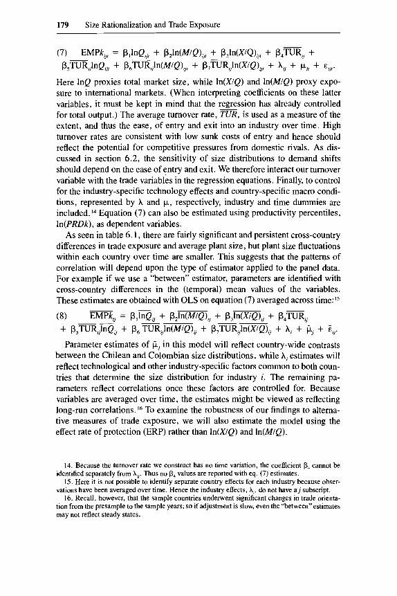
Here 1nQ proxies total market size, while ln(X/Q) and ln(M/Q) proxy exposure to international markets. (When interpreting coefficients on these latter variables, it must be kept in mind that the regression - has already controlled for total output.) The average turnover rate, TUR, is used as a measure of the extent, and thus the ease, of entry and exit into an industry over time. High turnover rates are consistent with low sunk costs of entry and hence should reflect the potential for competitive pressures from domestic rivals. As discussed in section 6.2, the sensitivity of size distributions to demand shifts should depend on the ease of entry and exit. We therefore interact our turnover variable with the trade variables in the regression equations. Finally, to control for the industry-specific technology effects and country-specific macro conditions, represented by A and F, respectively, industry and time dummies are included. l 4 Equation (7) can also be estimated using productivity percentiles, In(PRDk), as dependent variables.

As seen in table 6.1, there are fairly significant and persistent cross-country differences in trade exposure and average plant size, but plant size fluctuations within each country over time are smaller. This suggests that the pattems of correlation will depend upon the type of estimator applied to the panel data. For example if we use a “between” estimator, parameters are identified with cross-country differences in the (temporal) mean values of the variables. These estimates are obtained with OLS on equation (7) averaged across time:I5

Parameter estimates of p, in this model will reflect country-wide contrasts between the Chilean and Colombian size distributions, while A, estimates will reflect technological and other industry-specific factors common to both countries that determine the size distribution for industry i. The remaining parameters reflect correlations once these factors are controlled for. Because variables are averaged over time, the estimates might be viewed as reflecting long-run correlations. To examine the robustness of our findings to alternative measures of trade exposure, we will also estimate the model using the effect rate of protection (ERP) rather than ln(X/Q) and In(MlQ).

14. Because the turnover rate we construct has no time variation, the coefficient p, cannot be identified separately from A,,. Thus no p, values are reported with eq. (7) estimates.

15. Here it is not possible to identify separate country effects for each industry because obser- vations have been averaged over time. Hence the industry effects, A, , do not have a j subscript.

16. Recall, however, that the sample countries underwent significant changes in trade orientation from the presample to the sample years; so if adjustment is slow, even the “between” estimates may not reflect steady states.


An alternative estimator of equation (7) does not involve averaging over time. Rather, it identifies parameters by treating a single industry, country, and year as the unit of observation. If we control for technology differences with country-specific industry dummies, and we control for macro effects with country-specific time dummies, the resultant “within” estimates will reflect the time-series correlations of the size and productivity distributions with industry-specific trade policy. These estimates address the question of how much rationalization occurs within a country in the short run as trade exposure changes. They will be more sensitive to hysteresis effects than the “between” estimates, so entry and exit are likely to play a smaller role in the short run. Bear in mind also that this estimator will not pick up the dynamics of adjustment processes-all correlations are contemporaneous. Finally, given that the variable ERP does not vary through time, we are unable to check the robustness of our “within” regression by replacing ln(X/Q) and ln(M/Q) with the effective rate of protection.

6.4 Results: Between-Country Estimates

6.4.1 The Employment Size Distribution

Table 6.2 presents regression coefficients for the employment size distribution using the “between” estimator. Explanatory variables are listed on the left-hand side of the table and percentiles across the top. Each column in each panel summarizes a separate regression. The top panel was estimated using import and export shares as the measure of trade exposure and the bottom panel was estimated using effective rates of protection. Note that, overall, the fit as measured by adjusted R2 is very tight, and both trade patterns and turnover appear to matter a great deal. ’’ (F-statistics test the null hypothesis that all variables listed and industry dummies have zero coefficients.)

Looking across columns in the top half of table 6.2, one sees that an increase in import share is associated with a reduction in all size percentiles, controlling for the level of industry output. These results suggest that, contrary to the findings of many simulation models, the elasticity effects of import competition on plant size are not dominant. Rather, demand contraction, factor market effects, and other forces associated with increased import competition apparently lead to smaller plants.’* We defer the issue of whether this means efficiency losses accompany liberalization to section 6.4.3 below.

Notice next that large plants appear to contract relatively more in the face

17. Interestingly, the country dummy is insignificant in the employment regressions, suggesting that any cross-country contrast in the size distribution is associated with contrasts in the explanatory variables. (Country dummies in the productivity regressions of table 6.4 reflect differences in units of measurement, inter alia.)

18. Baldwin and Gorecki (1983) found similar effects in Canadian data, although they did not stress them in their analysis.


Table 6.2 Between Estimates of Employment Size Distribution' (absolute values of t-statistics in parentheses)

Percentile

10th 25th 50th 75th 90th

Trade Exposure Measured with Import and Export Shares

W / Q )

MQ) -

- TUR

TUR * In(M/Q)

TUR * In(X/Q)

TUR * In(Q)

Chile dummy

Mean of dependent variable

--

--

--

R 2 6 F (28,13)

- ERP

TUR

TUR * ERP

TUR * In(Q)

Chile dummy


R 2

6 F (26,15)

--

-~

- . l84* (2.59) - .204* (6.24) - .268* (3.81)

-7.60* (3.31)

(3.04)

(5.43)

.446*

.772*

.691* (4.65) - ,019 ( ,260)

2.47

,887 ,046

12.45

- .317* (2.78) - .333* (6.36) - .496* (4.40)

(3.86)

(2.82) 1.29*

(5.67) 1.21*

(5.09) ,055

(.473)

2.80

- - 14.17*

.663 *

.903

.074 14.57

- .432 (2.03)

(3.76) - ,414

10.02 (1.46) 1.11*

(2.31) 1.51*

(3.54)

(2.19) - .039

- .367*

(1.97)

.974*

(.179)

3.37

.842

.139 8.80

- .573* (2.24) - ,168 (1.43) - ,251 (1.W 13.43 (1.63) 1.39*

(2.64) ,695

(1.36) - .564 (1.06) - ,291 (1.12)

4.15

,866 ,167

10.46

-1.10* (2.98)

.004 (.022) ,129

(.353) 14.72 (1.23) 2.72*

(3.56) . I88

(. 254) - ,722 (.935) - ,037 (.097)

4.99

,765 ,242

5.76

Trade Exposure Measured with Effective Protection Rates

.244* .352* .361 ,332 ,368 (3.41) (2.52) (1.78) (1.97) (1.36)

.296* ,422 ,545 1.15* 1.24* (2.39) ( I .78) (1.58) (4.03) (2.70) 14.05* 19.08 21.96 43.73* 45.28 (2.33) (1.64) (1.31) (3.13) (2.03) - .707* - 1.05* - 1.01* - 1.04* - 1 . 1 1 (4.45) (3.43) (2.29) (2.84) (1.89) - .876* -1.18 - 1.41 - 2.67* - 2.73 (2.29) (1.62) (1.32) (3.03) (1.93)

,003 - .038 - .I13 - ,517 - ,474 (.014) (.097) (.198) (1.09) (.623)

2.47 2.80 3.37 4.15 4.99

.664 ,587 ,596 ,836 .647

.080 .153 ,222 ,185 ,296 4.12 3.24 3.33 9.02 3.89

~

%dustry dummies were included in the regressions but are not reported. *Significantly different from zero at the .05 level using a two-tail test.


of import competition, so even the market share effects of trade liberalization appear to be absent. This result is not as robust as the negative correlation between trade exposure and size, as will be seen presently. Nonetheless, possible explanations are worth listing. First, drawing on the simple analytics of section 6.3, it is possible that trade exposure actually reduces demand elasticities. Second, and more plausibly, it may be that imported goods do not compete with the kinds of goods small plants produce, so large plants bear most of the adjustment burden. Third, industries with large plants may be more effective at lobbying for import protection.

The coefficients on the interaction between TUR and ln(M/Q) are significantly positive, which implies that the size effect of trade exposure is more substantial in low-turnover industries. Given that import expansion is associated with output contraction, this is consistent with the theory reviewed earlier: More size adjustment occurs when exit is not easy. Alternatively, the results might be interpreted to mean simply that the discipline of foreign competition matters more in industries where the discipline of potential entry is less important. Here again, the larger effect for the higher percentiles is consistent with the hypothesis that imports compete more directly with big plants. In either case, the data support Buffie and Spiller (1986), Rodrik (1988a), and others who have argued that it is critical to take ease of entry into consideration when predicting the effect of regime changes on size distributions.

Turning next to export shares, one finds the direction of the effects is similar: High trade exposure is associated with smaller plant sizes, and the effect is strongest in industries with low turnover. This pattern is generally support- ive of the premise that both ln(X/Q) and ln(M/Q) measure exposure to foreign markets. However, the effect of ln(X/Q) now weakens as we move to higher percentiles, so most of the contrast between “open” and “closed’ markets appears to be showing up among small plants. This same pattern holds for the interaction between ln(X/Q) and TUR. We have no ready explanation for this finding, but it may indicate that small plants are relatively more important export suppliers.

Given import and export shares, larger industry-wide output levels have an effect on the size distribution that is qualitatively identical to that of trade exposure. Larger domestic production is associated with relatively more small producers, especially in low-turnover industries. However, it must be remem- bered that ln(Q) enters the variables In(X/Q) and ln(M/Q) negatively. Hence, the total effect of an increase in output holding M and X fixed is given by the sum of the output coefficient and the negative of the import and export coefficients. For example, a unit increase in ln(Q) holding X and M fixed shifts the 10th percentile rightward by .184 + .204 - .268 > 0. The negative coefficient on output in the regression equations implied that a proportionate increase in Q. X, and M is associated with a smaller size distribution of plants.

Since industry dummies are already included, the level of turnover only


controls for country-specific differences in turnover rates. These can be due to cross-country differences in product mixes within given industries, or to differences in credit markets and other determinants of sunk costs.19 The pattern that emerges is expected: High turnover is associated with a relatively large number of small plants.

To check the robustness of the findings concerning trade exposure and plant size, we next replace the trade exposure measures ln(X/Q) and In(M/Q) with the effective protection measure ERP.*O The coefficient on ERP in the regressions can be interpreted as the difference in size distributions that is correlated with differences in effective protection rates, controlling for country-wide plant-size differences, and for industry-specific effects.

Results are reported in the bottom half of table 6 .2 . Note first that there is a positive correlation of the employment size distributions with effective protection. Just as with the X/Q and M/Q measures of trade exposure, higher rates of effective protection are associated with larger plant sizes. Moreover, the size effect is less extreme in high turnover industries. In both these senses the results conform to the findings in the top half of table 6.2: Demand contraction and other effects associated with high trade exposure appear to dominate elasticity effects.

However, comparing the different size percentiles, one finds that the statistically significant effects of increased protection appear in the lower percentiles, which suggests that small plants expand at a relatively rapid rate when protection is increased. Contrary to our earlier findings, these results are consistent with the hypothesis that trade exposure increases demand elasticities, thereby inducing rationalization by forcing small plants to contract relatively more.

Finally, in the ERP regressions we see that larger domestic production and higher turnover are both associated with rightward shifts in the size distribution. Both of these patterns are present across all the percentiles. This same pattern was reported in the top half of table 6.2 for the 75th and 90th percentiles. However, the 10th through 50th percentiles tended to decline with increased output or turnover in the regressions based on In(X/Q) and In(M/Q). These do not strike us as important anomalies because, as discussed above, the size shift associated with output increases is positive for all table 6 .2 percentiles when X and M are held fixed. Also, our turnover variable is mainly useful in interaction terms; the level effects of entry barriers are essentially controlled for with industry dummies.

To summarize the robustness of the “between” estimates, we conclude that

19. Recall that Chile underwent a major financial crisis and restructuring in the early 1980s. 20. We also repeated these regressions using real output, rather than employment, as the mea-

sure of plant size. The qualitative results are very similar for the two measures. Overall, shifts toward smaller plants are associated with high trade exposure, especially in low-turnover industries. In the output size distribution, however, only the effect of export share was consistently significant.

184 Mark J. Roberts and James R. Qbout

the correlation between trade exposure and the employment size distribution is clearly negative in the long run, and the magnitude of the effect is clearly moderated by ease of entry or exit.21 However, whether small or large plants adjust more in percentage terms to increases in exposure depends on the measure of exposure that is used. Perhaps effective protection measures are most relevant for policy analysis, since these are most directly controlled by the government.

6.4.2 Predicted Employment Size Distribution under Alternative Trade Regimes

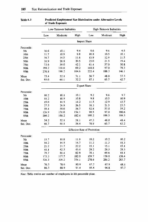
Given that the regression models use interaction terms between turnover and trade exposure, it is difficult to infer the magnitudes of predicted differences in the employment size distribution under alternative trade regimes. Ac- cordingly, table 6.3 presents predicted values of the employment size distributions based on regression results from table 6.2.

The top panel illustrates how the employment size distribution shifts as the import share rises, the middle panel illustrates how it shifts as the export share rises, and the bottom panel illustrates shifts with changes in effective protection. The left side of the table describes a low turnover industry while the right side corresponds to a high turnover industry. Within each panel, columns present “low”, “medium,” and “high” export or import shares.22 Finally, rows of the table give predicted employment levels for the 5th through 95th percentiles, as well as the mean and standard deviation of the employment distribution.

First, focusing on the size distribution for low-turnover industries, the leftward shift in the size distribution as import shares increase is marked. For example, the median plant size falls from 3 1.9 to 20.5 employees as the import share rises. This leftward shift is particularly large for the 75th, 90th, and 95th percentiles. Similarly, both the mean and the standard deviation drop substantially with increases in import share. Recall, however, that high turnover moderates the extent to which import shares reduce plant size. This appears in table 6.3 when one moves from the low-turnover to the high-turnover figures, especially among large plants.

Relative to import shares, export shares appear to covary less with the employment sizedistribution. Forexample, among low-turnoverindustries, the median plant size declines only from 27.3 to 26.5 employees as the export share increases. Also, although plants in high-turnover industries are generally

21. Similar results were obtained when plant-level output was used as a size measure instead of employment (see n. 20).

22. The “low-turnover” predictions assume the turnover rate associated with the 25th percentile of the turnover distribution, and “high-turnover” predictions assume the turnover rate of the 75th percentile. Low, medium, and high trade exposure measures correspond to the 25th, 50th, and 75th percentiles of their respective distributions.


Table 6.3 Predicted Employment Size Distribution under Alternative Levels of 'kade Exposure

Low-'hrnover Industries High-Turnover Industries

Low Moderate High Low Moderate High

Percentile: 5th 10th 25th 50th 75th 90th 95th

Mean Std. Dev.


Mean Std. Dev.


Mean Std. Dev.

Import Share

10.6 11.7 16.7 31.9 73.6

199.2 276.8

73.4 93.0

10.1 10.9 14.5 26.8 59.0

131.0 188.2

52.1 61.1

9.4 9.6 9.6 9.8 10.8 10.5

11.6 13.9 12.9 20.5 23.0 21.5 42.1 61.4 57.0 69.2 110.8 97.0

104.6 222.4 188.3

31.1 56.7 48.0 32.2 87.1 65.7

9.5 10. I 11.5 19.4 50.8 79.3

146.1

37.3 42.7

Export Share

10.2 11.2 15.0 27.3 59.4

124.9 200.2

54.2 66.7

10.1 10.1 10.9 10.8 14.5 14.2 26.8 26.5 59.0 58.7

131.0 134.1 188.2 182.4

52.1 51.1 61.1 58.4

9.2 9.6 9.8 10.5

11.5 12.9 18.3 21.5 52.8 57.0 90.5 97.0

188.2 188.3

47.3 48.0 70.9 65.7

9.7 10.9 13.7 23.3 59.2

100.6 188.3

48.4 63.2

Effective Rate of Protection

11.7 14.2 21.2 41.1 79.7

173.3 324.3

76.3 86.3

11.8 14.5 21.7 42.3 81.4

177.7 339.2

78.6 88.9

11.9 10.2 14.7 11.3 22.2 15.1 43.4 28.2 82.9 70.1

182.0 159.7 354.1 278.6

80.9 67.7 91.4 95.8

10.2 11.3 15.1 28.3 69.6

159.0 281.2

67.9 96.8

10.2 11.3 15.1 28.3 69.1

158.4 283.7

68.1 97.7

Note: Table entries are number of employees in kth percentile plant.


more concentrated in the lower employment ranges, changes in export shares appear to have little effect on location or shape of the distribution.

The bottom panel of table 6.3 reports predicted percentiles of the size distribution when the effective rate of protection is varied. The most substantial change occurs in the upper percentiles of the size distribution for low-turnover industries. Increases in the effective rate of protection are correlated with an increase in the size of the larger plants, but the increase is not as large as that associated with changes in import penetration.

6.4.3 Distribution of Labor Productivity

The empirical results thus far have shown that high trade exposure is associated with relatively small-scale production, controlling for other factors. Does this mean that trade exposure worsens productivity? To examine this issue more directly, we next apply our empirical model to the distribution of labor productivity across plants. This not only allows us to determine the overall direction of productivity shifts with trade exposure, it also speaks to such questions as whether shifts are concentrated among the least productive plants.

Table 6.4 reports “between-country’’ regression results for the percentiles of the labor productivity distribution. The top half of the table measures trade exposure with import and export shares while the bottom half uses effective rates of protection. The first result to notice is that significance levels are much lower than those associated with size distributions. Hence reductions in labor productivity do not obviously accompany reductions in scale. Notice next that differences in the import share between countries are positively correlated with differences in the percentiles of the productivity distribution, while the export share is negatively correlated. This negative correlation of exports and productivity could reflect the limitations of single-factor productivity measures: low labor productivity may be due to high labor intensity without im- plying low total factor productivity, since capital is not controlled for. More- over, the Heckscher-Ohlin models suggests that trade liberalization should stimulate exports of labor-intensive products, so this omitted variable bias in our productivity measure will be correlated with trade patterns.

Larger levels of industry output, holding import and export shares fixed, are correlated with a rightward shift in the labor productivity distribution. This could reflect increased capacity utilization or exploitation of scale economies in the larger market. High-turnover industries also have higher productivity levels. As was seen in the employment distributions, high turnover tends to reduce the magnitude of the import, export, and output correlations. Finally, the country dummy variable is positive and significant. This can simply reflect differences in the units of measurement of output. However, with the exception of the country dummy and output level among higher productivity plants, virtually none of the remaining coefficients is statistically significant. Unlike the employment size distribution, there is little evidence


Table 6.4 Between Estimates of Labor Productivity Distribution' (absolute values of &statistics in parentheses)

Percentile


TUR

TUR * In(M/Q)

TUR * In(X/Q)

TUR * In@) .

Chile dummy


--

--

~-

R z

6 F (28,13)

ERP

- MQ)

TUR

TUR * ERP

TUR * In@)

Chile dummy


~

_ _ -

_ _ -

R 2

6 F (26.15)

Trade Exposure Measured with Import and Export Shares

,158 ,239 .230 ,289 ,398 (.474) (.898) (.890) (1.08) (1.58)

~ ,271 - .258* - ,089 - ,045 -.186 (1.81) (2.16) (.764) (.372) (1.64)

(.775) ( I .44) (1.88) (2.38) (2.44) 8.26 8.81 7.26 9.27 6.46 (.754) (1.01) (. 854) (1.05) (.780)

( . S O ) (1.05) (1.18) (1.17) ( I .54) .910 .806 ,107 - ,064 .513

( I .40) (1.55) (.213) (.122) (1.04)

,260 .387 ,490 .643* .619*

- .389 - .592 - ,644 - ,667 - .824

- .495 -.516 - ,547 - ,618 - .312 (.708) (.926) (1.01) (1.10) (.589) 1.91* 1.88* 1.85* 1.72* 1.55*

(5.65) (7.00) (7.09) (6.32) (6.06)

4.56 5.02 5.52 6.07 6.58

.963 ,978 ,981 ,980 ,983 ,224 ,177 .I74 ,181 ,170

38.94 67.28 75.56 73.14 83.32

Trade Exposure Measured with Effective Protection Rates

,392 (2.04)

.788* (2.46) 36.08* (2.31)

(2.07) 2.49*

(2.51) 2.51*

(4.65)

4.56

- ,872

.967 .210

47.80

,296 (1.73)

.715* (2.50) 28.30 (2.03) - .588 (1.56) - 1.97*

(2.24) 2.48*

(5.13)

5.02

,976 .I87

65.73

.I61 ( I . O l )

,493 (1.86) 11.44

(.884) - ,031

(.089) - .880 (1.08) 2.52*

(5.63)

5.52

.981 ,174

81.35

.I43 ( . M I ) ,479

(1.71) 8.44 (.618) ,104

(.281) - .628 (.726) 2.56*

(5.43)

6.07

,980 ,183

76.25

,204 (1.21)

.552 (1.96) 12.05

(.879) -.147 (.399) - .868 (1.00) 2.45*

(5.18)

6.58

,979 ,184

76.12

&Industry dummies were included in the regressions but are not reported *Significantly different from zero at the .05 level using a two-tail test.


here that productivity differences across the two countries are related to trade exposure.

The bottom half of table 6.4 reports regression results using the effective rate of protection as the measure of trade exposure. Again, output and turnover are correlated with a rightward shift in the productivity distribution. In- creased trade protection is correlated with higher productivity, especially for the least productive plants, but once again, none of these coefficients is statistically significant. In short, there is no clear evidence that differences in trade exposure between sectors in Colombia and Chile are correlated with differences in the distribution of plant-level labor productivity.

6.5 Results: Within-Country Estimates

As reviewed in section 6.3, an alternative way to identify our model is to use the within-country temporal variation in the data. This approach picks up the short-run associations between trade exposure, output levels, and the size and productivity distributions. The top panel of table 6.5 presents results for the employment size distribution and the lower panel presents results for the productivity d i s t r i b ~ t i o n . ~ ~ (F-statistics test the null hypothesis that all reported variables, time dummies, and industry dummies have zero coefficients.)

6.5.1 Employment Size Distribution

Fluctuations in import shares show a negative association with plant sizes, just as in all the “between” country regressions. Now, however, this association is so weak statistically that it makes little sense to talk of short-run rationalization effects. Because we are limiting the “within” model to contemporaneous effects, we find this low significance unsurprising.

More surprisingly, time series fluctuations in export shares correlate positively with the percentiles of the size distribution, although they are negatively correlated with percentiles in the “between” regressions. Though weaker than in table 6.2, these correlations are still statistically significant. So in the short run, output growth due to export share expansion is associated with relatively rapid employment growth. In terms of rationalization, the growth in employment is concentrated among large plants. We see no obvious explanation for this contrast between the “within” and the “between” results.

The coefficients on the output variable indicates that the correlation of in-

23. The “within” estimator, unlike the “between” estimator, permits us to test the null hypothesis that the same relationship between size and trade exposure holds in all industries. But to do so, we must drop our time dummies and our turnover index. Not surprisingly, for this restricted version of the model the hypothesis of common slope coefficients across industries can be rejected for all the employment and productivity percentiles. Specifically, the F( 120,210) statistics for the loth, 25th, 50th, 75th, and 90th employment percentiles are 5.12, 9.03, 10.60, 9.10, and 7.63, respectively. The same statistics for the productivity percentiles are 2.81, 2.70, 1.94, 2.47, and 3.27.


dustrial output with plant sizes is generally positive. This reflects a combination of output adjustments by incumbents and entry or exit. However, given that most turnover takes place among small plants, shifts in the higher percentiles reflect mainly the expansion and contraction of incumbents (Roberts 1989; vbout 1989). Finally, in industries where turnover is high, the positive correlation between output and size is relatively muted.

Overall, the patterns of contemporaneous correlation between the percentiles of the employment size distribution are much less systematic than the between country estimates. Systematic rightward or leftward movements of the size distribution are not obvious in the regression results. This suggests that while the across-country differences in trade exposure are correlated with differences in the entire size distribution of plants, the time-series differences in trade appear to have a more random effect on plants within the size distribution. This may mean that differences in the plant-size distribution between the countries reflect underlying structural differences in the size of markets, openness to trade, and other factors. In contrast, time-series fluctuations in the size distribution within each industry and country reflect idiosyncratic as- pects of the market and time period.

6.5.2 Labor Productivity Distribution

The bottom half of table 6.5 reports results for the labor productivity distribution using the within-country variation. Import share has no significant effect on the shape of the distribution. In contrast, an increase in the export share is positively and significantly correlated with the loth, 25th, and 50th percentiles of the productivity distribution but negatively correlated with the 75th and 90th percentiles. That is, higher export shares are correlated with higher productivity for the less productive plants but lower productivity for higher productivity plants.

Expansion in output over time leads to productivity improvements. This can result from either increased use of capital or scale economies in high output periods. Finally, as we have seen throughout this paper, the import, export, and output correlations are lower in magnitude in high-turnover industries. In particular, the turnover results could arise if high-turnover industries are less capital intensive or have technologies with less scale economies. De- mand fluctuations in these industries then have less effect on an individual plant’s labor productivity and thus less effect on the distribution across plants.

Overall, the “within” estimator indicates little evidence of rationalization with variation in trade exposure over time. The productivity changes over time are largely explainable with variation in capital utilization.

6.6 Summary

It is often argued that when domestic markets are imperfectly competitive, increased exposure to global markets should rationalize production. Such ex-

190 Mark J. Roberts and James R. @bout

Table 6.5 Between Estimates of Employment Size and Productivity Distribution' (absolute values of &statistics in parentheses)

Percentile


TUR * In(X/Q)

TUR * In(Q)


R 2

6 F (63,314)

MMiQ)

WOQ)

MQ)

TUR * ln(M/Q) -

TUR * ln(X/Q)

TUR * ln(Q)


R 2

-

6 F (63,314)

Employment Size Distribution

- ,048 (.812) .035*

(2.35) ,163

(1.58) .226

(1.19) - ,091 (1.83) - ,577 ( I .76)

2.48

,805 ,072

25.66

,010 (.144) ,007

(.417) .270*

(2.27) - ,047

- ,026 (.215)

(.452) - .776* (2.05)

2.82

.902 ,083

56.06

- .168* (2.06) - .042* (2.04)

,165 (1.17)

,463 (1.77)

.146* (2.12) - ,306

(.679)

3.40

,932 .099

82.78

-.I15 (1.03)

.071* (2.57)

,349 (1.82)

,195 (.551) - .243* (2.61) - ,784 (1.29)

4.19

.925

.133 74.98

-.i20 (1.09)

.061* (2.19)

.624* (3.26)

,178 (.502) - .214 (2.30) - 1.25* (2.07)

5.02

,936 ,133

88.76

Labor Productivity Distribution

.007 (.066) .053

(1.89) .714*

(3.68) - .003 (.008) - ,101 ( I .07) - ,890 (1.44)

4.33

,986 .I35

418.55

- ,066 (.712) .076*

(3.25) .686*

(4.26) .I82

(.612) - .187* (2.39)

( I .63)

4.78

- .837

,991 ,112

668.55

- ,011 (. 120) .069*

(2.95) .982*

(6.07) ,067

(.225) -.187* (2.38) - 1.85* (3.59)

5.27

,992 ,133

706.12

- ,046 (.520) - .056* (2.55)

.896* (5.89)

,280

.258* (.995)

(3.50) - 1.55*

(3.21)

5.83

,993 ,106

837.12

.044 (.432) - .055* (2.12)

I .29* (7.25) - ,017 (.052) ,149

( I .73) -2.93*

(5.18)

6.35

,990 ,124

620.30

Separate industry dummies and time dummies for each country were included in the regressions but are not reported. *Significantly different from zero at the .05 level using a two-tail test.


posure is believed to increase the elasticity of demand perceived by domestic producers, which in turn should shift production toward the large, efficient plants. The rationalization effects should be especially marked when there are low barriers to entry and exit because inefficiently small plants will be induced to shut down. This paper is the first attempt we know of to confront these theories of rationalization with actual data on the size distribution of plants from developing countries.

Several striking results emerge. First, increased exposure to import competition appears to clearly reduce the size of all plants in both the short run and the long run, but especially in the latter. Whether large plants shrink relatively less depends on the way in which we measure exposure to world markets: Increases in import shares are associated with relatively rapid shrinkage by large plants, but reductions in effective protection correlate with relatively little shrinkage by large plants. Either way, it appears that models that predict trade liberalization will increase average plant size in import-competing sectors do not describe recent Chilean and Colombia experiences. This may mean that productivity improvements have not accompanied liberalization, but our findings on this issue are not strong enough to warrant much confidence in this conclusion.

Second, as theory suggests, it makes a great deal of difference whether one is analyzing industries with high or low entry barriers. The effects of changing output levels, import shares, export shares, and effective protection rates are systematically moderated by the possibility of easy entry or exit. One interpretation is that there is less role for output adjustment by incumbent plants when the number of plants adjusts to demand shifts. Alternatively, our results could simply mean that high turnover reflects competitive pressure and reduces the marginal impact of foreign competition on market structure.

Third, the “long-run” correlations of trade regimes and size distributions are quite different from the short-run year-to-year correlations. Not only are the effects of trade exposure stronger in the long run, but the correlations of export shares change sign. The short-run correlations show exports associated with relatively small plants. We trust the long-run figures more, because we limited our short-run analysis to simultaneous correlations and have not at- tempted to model the dynamics of adjustment. Nonetheless, the short-run findings suggest caution in extracting policy recommendations from our figures.

This paper is a first step in the direction of micro-based examinations of the rationalization hypothesis. Though suggestive, much remains to be done. Aside from modeling the dynamics of adjustment, we hope to study the relationship between average costs and size and the degree to which plants adjust costs endogenously with changes in the trade regime.

192 Mark J. Roberts and James R. 'Qbout

References

Baldwin, J. R., and P. K. Gorecki. 1983. Trade, Tariffs, and Relative Plant Scale in Canadian Manufacturing Industries: 1970-1979. Economic Council of Canada, Discussion Paper No. 232.

Bergstrom, T., and H. Varian. 1985. When are Nash Equilibria Independent of the Distribution of Agents' Characteristics? Review of Economic Studies 52: 7 15-18.

Bhagwati, J. 1988. Export Promoting Trade Strategy: Issues and Evidence. World Bank Research Observer 3:27-58.

Brown, D. 1989. Tariffs and Capacity Utilization by Monopolositically Competitive Firms. Tufts University Discussion Paper No. 89-108.

Buffie, E. , and P. Spiller. 1986. Trade Liberalization in Oligopolistic Industries. Jour- nal of International Economics 20:65-8 1.

Condon, T., and J. de Melo, 1990. Industrial Organization Implications of QR Trade Regimes: Evidence and Welfare Costs. World Bank. Typescript.

Corbo, V. 1985. Reforms and macroeconomic adjustments in Chile during 1974-84. World Development 132393-916.

Cubillos Lopez, Rafael, and Luis Alfonso Torres Castro. 1987. La Proteccion a la Industria en un Regimen de Exenciones. Revista de Planeacion y Desarrollo 19:45- 100.

Devarajan, S. , and D. Rodrik. 1989a. Trade Liberalization in Developing Countries: Do Imperfect Competition and Scale Economies Matter? American Economic Re- view, Papers and Proceedings 79: 283-87.

. 1989b. Pro-competitive Effects of Trade Reform: Results from a CGE Model of Cameroon. Harvard University. Typescript.

Dixit, A., and V. Norman. 1980. Theory of International Trade. Cambridge: Cam- bridge University Press.

Dutz, M. 1990. Firm Adjustment to Trade Liberalization. Princeton University. Type-

Eastman, H. C., and S. Stykolt. 1966. The Tariff and Competition in Canada. To- ronto: University of Toronto Press.

Garcia, J. 1988. The Timing and Sequencing of a Trade Liberalization Policy: The Case of Colombia. World Bank. Typescript.

Harris, R. 1984. Applied General Equilibrium Analysis of Small Open Economies with Economies of Scale and Imperfect Competition. American Economic Review

Helpman, E., and P. Krugman. 1985. Market Structure and Foreign Trade. Cam- bridge, Mass.: MIT Press.

Horstmann, I., and J. R. Markusen. 1986. Up the Average Cost Curve: Inefficient Entry and the New Protectionism. Journal of International Economics 20: 225-48.

Jovanovic, B. 1982. Selection and the Evolution of Industry. Econometrica 50, 649- 70.

Lancaster, K. 1984. Protection and Product Differentiation. In Monopolistic Competi- tion and International Trade, ed. H. Kierzkowski, 137-56. Oxford: Oxford Univer- sity Press.

Markusen, J. 1981. Trade and the Gains from Trade with Imperfect Competition. Jour- nal of International Economics 11 531-5 1.

Melo, J. de, and D. Tarr. Forthcoming. A General Equilibrium Analysis of US. Trade Policy. Cambridge, Mass.: MIT Press.

Pack, H. 1989. Industrialization and Trade. In Handbook of Development Economics, ed. H. Chenery and T. N. Srinivasan, vol. 1. Amsterdam: North-Holland.

script.

74: 1016-33.


Roberts, M. 1989. The Structure of Production in Colombian Manufacturing Indus- tries. World Bank. Typescript.

Rodrik, D. 1988a. Imperfect Competition, Scale Economies and Trade Policy in De- veloping Countries. In Trade Policy Issues and Empirical Analysis. ed. R. Baldwin. Chicago: University of Chicago Press.

. 1988b. Closing the Technology Gap: Does Trade Liberalization Really Help? Harvard University. Typescript.

Tybout, J. 1989. Entry, Exit, Competition and Productivity in the Chilean Industrial Sector. World Bank. Typescript.

Comment Robert E. Lipsey

The basic question that motivates this study is whether trade liberalization in developing countries, or liberalization of the economy in general, increases the efficiency of production. That is the issue the authors raise in the introduc- tion, it is of great interest to development and trade economists, and it was apparently the question that motivated the World Bank study from which this paper is derived.

A major novelty of the paper is the use of establishment data from censuses of manufactures for Chile and Colombia, data that are rarely available to re- searchers outside the statistical agencies themselves. They are the only type of data that could be used to study size distributions, as is done in this paper, and they have the potential for examining many other broader issues involved in the study of the effects of trade policy.

This paper, described by the authors as a first step in the analysis of their exceptionally rich data set, focuses on one aspect of that broader topic: an attempt to explain the shape of the distribution of manufacturing plants by size and the distribution by output per worker.

One reason for relating trade policy to the size distribution of firms is that much of the theoretical literature and simulation models of trade policy assume the importance of scale economies. Yet, as the authors point out, the empirical literature has not confirmed the efficiency effects of trade liberalization and, in particular, has not confirmed the channel of efficiency gains through effects on the size distribution of firms.

The description of the data brought my mind back to a paper by Patricio Meller, based on the 1967 Chilean Manufacturing Census, that confirmed for that country what had been found for the United States: great heterogeneity of establishments with respect to size and measured productivity within appar-

Robert E. Lipsey is a professor of economics, Queens College and the Graduate School and University Center, the City University of New York. He is also a research associate and director, New York Office, of the National Bureau of Economic Research.


ently narrowly defined industries. ’ Striking findings there were that 75 percent of establishments operated at a level of efficiency more than 50 percent below that of the most efficient in their four-digit industries and that neither size, nor capital/labor ratios, nor skill ratios were systematically different between efficient and inefficient firms in the same industry. However, the dispersion was much smaller among large firms. In the small firm group (5-9 persons), 46 percent of establishments were less than a third as efficient as the most efficient establishments in their size group. Among large firms (100 or more), only 6 percent were less than a third as efficient as the firms on the efficiency frontier.

What can explain the survival of apparently inefficient enterprises? Meller suggested various imperfections of factor and commodity markets, especially in the circumstances of 1967, but also pointed out that even within four-digit industries, establishments are producing goods that are not substitutes. That is partly a matter of geographical isolation, but also includes differences in quality of product and in the range of products produced.

Two of the assumptions in the theoretical presentation in the Roberts and Tybout paper seem to contradict Meller’s interpretation of his results. One is the assumption that “domestically produced goods are perfect substitutes.” The other is the assumption that “firms with low marginal costs are relatively large.” The authors disavow the size-marginal cost relation as an empirical regularity but use it because it illustrates the working of “most analytical and simulation models .” Meller reported that “it cannot be established empirically that one size group of industrial establishments is more efficient from a technical viewpoint than another size group. . . . [Llarger establishments are more technically efficient than smaller establishments only in two industries.” The present paper deals with a period in which the Chilean economy was much less protected from foreign competition and in which domestic markets were far less regulated than in 1967,* but it would be useful for interpreting the present results to know whether these earlier findings still applied.

I did not find the theoretical framework that begins the paper very helpful in interpreting the results. The authors, too, need to step outside it from time to time in order to arrive at more intuitive interpretations of their results. An example is the assumption in the theoretical framework that while domestic products are imperfect substitutes for imports, all domestic goods in a three- digit industry are perfect substitutes. In explaining why import liberalization appears to affect large firms more than small ones, Roberts and Tybout sug-

1. Patricio Meller, “Efficiency Frontiers for Industrial Establishments of Different Sizes,” Ex- plorations in Economic Research, vol. 3 , no. 3 (New York: National Bureau of Economic Re- search, 1976).

2. James Tybout, Jaime de Melo, and Vittorio Corbo, “The Effects of Trade Reforms on Scale and Technical Efficiency: New Evidence from Chile,” World Bank, Washington, D.C. (June 1989), manuscript.


gest, quite plausibly but in contradiction to the assumption, that imported goods do not compete with the kind of goods small plants produce but do compete with the output of large plants.

The main substantive results are from what is referred to as “between- country estimates.” These compare the size of plant at each of five percentiles in Colombia with the size of the plant in the same industry at the same percentile in Chile. Plant size in an industry at a percentile, such as the 10th or the 50th, is then related to a number of industry variables that may differ between the countries. These includes measures of trade exposure (export/production and import/production ratios and effective protection rates), of industry output, and of the turnover of firms in an industry.

The between-country results are described in the text as if they involved changes in the variables but they are, of course, differences between the countries. The authors interpret these as the long-run effects that would follow from changes in the independent variables, but it is not always obvious that another interpretation would not be as plausible. For example, higher import ratios in an industry in a country seem to be associated with smaller plant sizes. That association is referred to as resulting from a contraction of plants in the face of greater import competition. Another explanation that is equally plausible, I think, is that imported components can be a substitute for labor input, and therefore the higher the ratio of imports to output in an industry, the smaller the employment for a given output.

High ratios of exports to output are also associated with smaller plant employment size, particularly among smaller plants. The authors suggest that small plants may be “relatively more important export suppliers.” While that is a possibility, it would be surprising in view of the common belief that large firms are responsible for a disproportionate share of exports in most countries. Another possibility is that the plants at the low end of the employment size scale are more often assembly-type operations with large imports of components and large exports of finished products, but small employment relative to their output.

I do not mean to suggest that these interpretations are particularly more convincing than those offered by the authors. My point is that results of comparisons of size distributions are subject to a variety of equally plausible interpretations.

The measures of turnover used in the analysis here are industry characteristics rather than variables to be affected by liberalization. Exits and entrances would be extremely interesting to observe and study as a consequence of liberalization rather than only as an industry characteristic. Who exits the industry? If they are small firms, are they inefficient small firms? Are new entrants small when they enter? It would also be interesting to study the relation of exits and entrances to the size distribution of establishments. A rise in the average output at the 10th percentile could reflect gains in output by all the


firms in the lowest 10 percent. That seems to be the author’s usual interpretation of the numbers. However, it could also reflect the disappearance of a large number of small firms, so that the ones now at the 10th percentile are the ones that were at the 20th percentile before. Those would be very different events, and it would be worth while to distinguish between them. Some of these issues are discussed elsewhere by T y b ~ u t , ~ but the results do not seem to get incorporated into the present discussion.

Another section of the paper deals with between-country differences in what is referred to as productivity or labor productivity. The authors point out that this is a partial productivity measure, but the point deserves emphasis. Since capital intensity is not controlled for, variations in labor productivity imply nothing about efficiency or about the marginal costs referred to earlier in the paper. It is conceivable that high labor productivity plants are simply capital-intensive operations, and there is no assurance that high capital intensity represents efficiency, particularly in a developing country. As the authors point out in commenting on the negative correlation between export shares and labor productivity, “trade liberalization should stimulate exports of labor- intensive products,” that is, by this measure, low productivity products. What can we conclude, then, from this analysis?

Another aspect of liberalization that might be considered in future work is the degree of openness to foreign direct investment. Studies for Mexico seem to suggest that the presence of foreign firms in an industry can have a substantial effect on the rate of growth of productivity or convergence toward developed-country productivity level^.^ Foreign direct investment does not play the same role in manufacturing in Chile and Colombia as it does in Mex- ico, but the effect may be worth investigating, especially if the census data distinguish foreign-owned establishments.

On the whole, the results presented here whet one’s appetite for further study of these data. My feeling is that not much can be squeezed from further study of distributions of firms and that the most interesting results will come from the future work that will take advantage of the longitudinal aspect of the data. One would like to know which firms and establishments are growing and declining with trade liberalization or other changes in economic policy or external economic forces. The studies that have come from the U.S. Census Bureau’s program of analysis of longitudinal census data encourage me to believe that this project has potential payoffs that are not yet evident in this first report, and that is something to look forward to.

3. James Tybout, “Entry, Exit, Competition, and Productivity in the Chilean Industrial Sector,” World Bank, Washington, D.C. (May 1989), manuscript.

4. See Magnus Blomstrom and Edward N. Wolff, “Multinational Corporations and Productivity Convergence in Mexico,” NBER Working Paper no. 3141, October, and Magnus Blomstrom, Foreign Investment and Spillovers: A Study of Technology Transfer to Mexico (London: Rout- ledge, 1989).


Comment Peter A. Petri

This is a novel and interesting paper, one of the few studies that I know that examine the effects of trade exposure using a firm-level, microeconomic dataset. It is also timely and important, given how much money and effort is cur- rently being invested by developing countries and the “terrible twins” (the IMF and the World Bank) in outward-oriented development strategies. Fi- nally, it seems to produce a very surprising (though frankly not entirely convincing) result.

Broadly, three types of static production gains can follow from trade liberalization: intersectoral resource shifts from inefficient to efficient sectors, in- trasectoral resource shifts from inefficient to efficient firms, and intrafirm resource shifts from inefficient to efficient activities. This paper addresses the middle tier of these effects, the efficiency gains associated with changes in the market share of different firms. The authors use a theoretical model to associate efficiency with firm size, and they then check to see whether trade exposure leads to higher market shares for larger firms (i.e., greater concentration).

The surprise is that greater trade exposure tends to shift the size distribution toward smaller rather than larger firms. This runs against the predictions of the paper’s simple oligopoly model, which suggests that demand changes that represent greater openness should lead to a consolidation of industry output in the hands of larger, more efficient firms. There are two alternatives: The results may be wrong, or the theory may be inappropriate.

Consider first the strength of the evidence. The authors examine the effect of trade exposure on industry structure by running regressions of firm size (the independent variable) on various measures of trade exposure, both en- tered separately and in interaction with a “turnover” (ease-of-entry) variable. One factor that makes the results difficult to interpret is that the direct and interaction terms for a given trade exposure measure typically have opposite signs, and therefore the net effect of trade exposure on concentration is smaller than suggested by its direct coefficient alone. Fortunately, the authors do show net effects in table 6.3, which simulates changes in trade exposure holding other things constant. It shows that in low turnover industries (where the strongest effects are found), shifting from low to high trade exposure reduces the median firm’s employment from 31.9 to 20.5 using the import penetration measure, from 27.3 to 26.5 using the export-output measure, but increases it from 41.1 to 43.4 using the ERP measure. No statistical brackets are given for these estimates, but it would seem that only the import penetration results imply statistically significant changes. This raises the question, to

Peter A. Petri is the Carl Shapiro Professor of International Finance, and Director of the Lem- berg Program in International Economics and Finance, in the Department of Economics, Brandeis University.

198 Mark J. Roberts and James R. ‘Qbout

which I return later, whether something else might explain the relationship between high import exposure in particular and the absence of large firms.

A second point concerns the nature of the dataset. The long-term analysis, which is the only one that appears to provide statistically significant results, essentially compares industry size distributions in Colombia and Chile, rather than changes in the size distribution that might have resulted from a liberalization program. Both Colombian and Chilean data exclude firms with fewer than 10 employees. Consider the implications of this floor in the following thought experiment. Assume that before Chile liberalized its trade, firms in both Chile and Colombia were distributed uniformly between 10 and 100 employees. Suppose now that the Pinochet “treatment” reduced employment equally (say, by one half) in firms of every size category. We would therefore expect to see firms ranging from 5 to 50 employees in Chile-but the Chilean census forces all firms below 10 employees to “exit”! Comparing the tops of the distributions across the two countries, we will see the full 50 percent decline, but at the bottom both Chile and Colombia have 10-employee firms (0 percent decline). In between, the 25th percentile firm will appear to shrink by 38 percent, and in general, the decline will appear smaller near the bottom of the distribution. Since table 6.3 suggests that many firms are clustered near the 10-employee floor, one wonders to what extent the results are an artifact of censoring.

Now consider the appropriateness of the theory. Were the large firms that may have disappeared in Chile more efficient than small firms? Unfortunately, there are apparently not enough data to examine the relationship between total factor productivity and firm size, and since factor proportions typically vary with firm size, labor productivity cannot serve as a proxy. Meanwhile, as the authors carefully note, the theoretical connection between size and efficiency is established only for the rather narrow specification of the paper-Cournot interactions in a homogeneous product oligopoly model.

The authors propose several sensible alternative explanations based on the assumption that the products produced by different-sized firms are heteroge- neous-a very plausible explanation in light of the great variability that we observe in various firm statistics even within four-digit industrial classifica- tions. One possibility is that smaller firms are better able to survive foreign competition because they occupy niche markets, protected by natural barriers such as geography. This point nicely complements the analysis of U.S. steel markets elsewhere in this book; minimills have fared much better against imports than large integrated producers. A further related possibility is that the “missing” large firms in Chile are not missing because of greater import penetration, but because of third factors (say, the absence of some local raw ma- terial) that make the country uncompetitive in that product that the large firms would have made and that therefore also lead to higher import penetration.

Finally, consider the implications of the paper for liberalization. Methodo- logical quibbles aside, there seems to be evidence here to support the paper’s central point, that it is futile to expect large gains from scale effects in import-


besieged industries. But should we be looking for large gains from trade within industries that are knocked out by foreign competition? The real gain here is that resources are released. There may still be plenty of rationalization elsewhere-across firms classified by a better correlate of efficiency, within firms, and across sectors. The paper does not address these questions directly, but it presents intriguing evidence that such rationalization is happening. The shrinkage of the manufacturing sector analyzed in the paper suggests that the action is elsewhere-perhaps in grapes in Chile and other, more troublesome agricultural products in Colombia. I hope that in future work the authors will look deeply into these and other data to address the issue of efficiency. This is a stimulating beginning for an important, if difficult, journey.

This Page Intentionally Left Blank

size rationalization and trade exposure in developing

Documents