siting wind turbines to minimize raptor … partly derived from gps/gsm telemetry data transmitted...

1

SITING WIND TURBINES TO MINIMIZE RAPTOR COLLISIONS AT SUMMIT

WINDS REPOWERING PROJECT, ALTAMONT PASS WIND RESOURCE AREA

K. Shawn Smallwood and Lee Neher

8 December 2016

EXECUTIVE SUMMARY

Map-based collision hazard models were prepared as a set of tools to help guide the careful siting

of proposed new wind turbines as part of the repowering effort at Summit Winds in the Alameda

County portion of the Altamont Pass Wind Resource Area (APWRA). Similar collision hazard

models were prepared for the Tres Vaqueros and Vasco Winds repowering projects in Contra

Costa County and for the Patterson Pass, Golden Hills, Golden Hills North and Sand Hill

repowering projects in Alameda County. After three years of fatality monitoring following

construction, it was found that the repowering of Vasco Winds reduced fatalities of raptors as

well as all birds as a group. This newest set of models for Summit Winds benefit from the

lessons learned at Vasco Winds, as well as from many additional data collected through 2015

and the emergence of dependent variables and predictor variables that we believe result in

superior collision hazard models. The new models were derived from an additional four years of

fatality monitoring data, including monitoring with much shorter fatality search intervals at

repowered, modern wind turbines as well as at some old-generation wind turbines. And like the

models developed for Sand Hill and Golden Hills North, the golden eagle collision hazard model

was partly derived from GPS/GSM telemetry data transmitted by golden eagles (Aquila

chrysaetos) flying within the APWRA.

Our collision hazard model for golden eagle was derived from 121,259 GPS/GSM telemetry

positions within the APWRA, from thousands of behavior records made during visual scans

across many stations in the APWRA 2012 through 2015, and from fatality rates at monitored

wind turbines from 1998 through 2015. Our collision hazard models for red-tailed hawk (Buteo

jamaicensis) and American kestrel (Falco sparverius) were derived from thousands of behavior

records and from estimates of fatality rates at wind turbines. Our collision hazard model for

burrowing owl (Athene cunicularia) was derived from 5 years of burrowing owl surveys in 46

plots located throughout the APWRA, as well as from estimates of fatality rates at wind turbines.

Based on our models, we predict fatality reductions of golden eagles, red-tailed hawks, American

kestrels, burrowing owls and all birds as a group. Given the airspace that will be opened up to

safe golden eagle traffic, we believe the golden eagle fatality rate will lessen even though

collision risk is predicted to be relatively high at some turbine locations. American kestrel

fatalities will likely lessen due to the elimination of the many small wind turbines that not only

caused collision fatalities but also entrapped kestrels in hollow tubes of the lattice towers and

within the turbine machinery. Burrowing owl fatalities should decline by at least 90%. Based on

our experience at Vasco Winds, the fatality rates of bats might increase from the old wind

turbines at Summit Winds. However, the fatality monitoring performed at Summit Winds was

inadequate for detecting bat fatalities so it will be difficult to determine the repowering project’s

effects on bats.

2

INTRODUCTION

Salka LLC plans to install up to 26 wind turbines as part of its Summit Winds repowering project

in the Alameda County portion of the Altamont Pass Wind Resource Area (“APWRA”),

California. Careful siting of wind turbines is one of the principal measures available to minimize

raptor fatalities caused by collisions with the turbines (Smallwood and Thelander 2004,

Smallwood and Karas 2009, Smallwood and Neher 20010a,b, Smallwood et al. 2016). The

objective of this approach is to carefully site new wind turbines to minimize the frequencies at

which raptors of various species encounter the wind turbines while flying, but most especially

while performing specific types of flight behaviors, such as golden eagles chasing or fleeing

other birds or flying low across ridge-like topographic features, or red-tailed hawks or American

kestrels hovering or kiting in deflected updrafts. In this study we developed simple Fuzzy Logic

(FL) models (Tanaka 1997) of raptor activity quantified from behavior data collected across the

APWRA between 13 November 2012 and 29 October 2015, and at behavior studies performed at

Sand Hill sites between 30 April 2012 and 5 March 2015 and Patterson Pass between 15 October

2013 and 24 September 2014. The behaviors used in the modeling effort were derived from the

results of Smallwood et al. (2009b), and an example application of the FL modeling approach

can be seen in Smallwood et al. (2009a, 2016).

The Fuzzy Logic approach is a rule-based system useful with noisy data or with zero-dominated

data sets, and is applied to events occurring within classes that are assumed to have graduated

rather than sharp boundaries (Tanaka 1997). The rules consist of assigning likelihood values of

an event occurring, which in the case of this study would be the likelihood of a bird performing a

specific behavior within a cell of an analytical grid laid over the project area. Likelihood values

can range 0 to 1 for each predictor variable, depending on how far a value of the predictor

variable differs from the mean where the event has been recorded. The magnitude of each

deviation from the mean is assessed by the analyst based on error levels, data distribution, and

the analyst’s knowledge of the system. In our case, the events were of birds flying over terrain

characterized by suites of slope conditions, or of fatalities at wind turbines associated with

specific slope conditions, or of burrowing owl burrows associated with specific slope conditions.

The study goal was to accurately predict the locations where golden eagles, red-tailed hawks,

American kestrels and burrowing owls are most likely to perform flight behaviors putting these

species at greater risk of collision with wind turbines, so that new wind turbines can be sited to

avoid these locations to the degree reasonably feasible. Achieving this goal depended on our

understanding of how these species use terrain and wind, and how they perceive and react to

wind turbines. It also depended on understanding patterns of fatality rates in the APWRA, so we

also developed fatality rate models for golden eagle, red-tailed hawk, American kestrel, and

burrowing owl. Our model results were interpreted in tandem with Smallwood’s familiarity with

conditions associated with proposed wind turbine locations. By carefully siting the wind

turbines to minimize collision risk, the Summit Winds project should prove safer to raptors than

the wind turbines being replaced. The Summit Winds micro-siting also benefits from what was

learned at the Vasco Winds repowering project, which was micro-sited using a similar approach

and monitored for collision fatalities for three years (Brown et al. 2013, 2014, 2016).

3

Our map-based models are intended to help guide micro-siting. The models are only as

predictive as our understanding of wind turbine collisions and our ability to measure terrain

features bearing on collision risk. Although research and monitoring efforts in the APWRA have

set the pace worldwide (Orloff and Flannery 1992, Smallwood and Thelander 2008, Smallwood

et al. 2009b, Brown et al. 2016, ICF International 2016), there remains considerable uncertainty

over collision mechanisms. Certain behavior patterns correlate with collision fatality rates

(Smallwood et al. 2009b), but correlations are often confounded by the unmeasured, unobserved

factors. And whereas we know that collision risk is influenced by interactions between

landscape and wind, wind turbine micro-siting cannot be guided by anything more detailed than

measurable terrain features and prevailing wind directions. Assuming that the prevailing wind

directions are primarily from the southwest and secondarily from the northwest, and assuming

that the avian behavior and fatality data reflect these prevailing wind directions, we weighted

terrain features for collision risk based on whether wind turbines would be sited on or atop them.

However, when the wind shifts directions to the northeast or from the southeast, as examples,

then the birds shift their activity patterns and collision risks also change. There is no way for us

to micro-site wind turbines to minimize risk posed by all wind directions.

As another example of the limitations of our models, we examined the locations of golden eagle

model prediction failures – sites of existing or past wind turbine sites where collision risk was

predicted lowest but where fatality rates were relatively high. A pattern that quickly emerged

from these sites was their occurrence on steeply declining ridge features, which is a terrain

condition that we have not measured and could not incorporate into a model. We measured

slope (elevation change relative to distance change) within analytical grid cells and across entire

slope faces from valley bottom to ridge crest, but we did not measure slope along ridge features

because this measurement did not occur to us until examining the model prediction failures. If

we had another month to prepare collision hazard models, we could measure and use ridgeline

slopes. Of course, any remaining model prediction failures would likely lead us to additional as-

yet-unmeasured terrain features. Our models express our current understanding and ability to

measure collision factors, and should be interpreted in combination with expert opinion.

Assumptions and limitations aside, we feel that this iteration of collision hazard models in the

APWRA qualifies as our best and most predictive. We recommend siting the new wind turbines

as far as reasonably feasible from hazard classes 3 and 4, but we also recommend considering

expert input on the siting of each wind turbine to account for factors not considered in the

models. As a general rule, we recommend not siting wind turbines in relatively low terrain, or in

ridge saddles, breaks in slope or on terrain located east (prevailing downwind) of major ridge

saddles or breaks in slope.

METHODS

On-site Assessments

One of us (Smallwood) visited the proposed repowering project area to assess the collision

hazard associated with proposed wind turbine sites. Smallwood visited the sites proposed in the

initial layout in 2014, and except for turbine 28, he visited the sites proposed in the most recent

layout in October 2016. Smallwood rated collision hazard on a scale of 0 to 10 using criteria

4

adopted by the Alameda County Scientific Review Committee in 2007/2008 and 2010. He

recommended changes to the original turbine layouts prior to the development of collision

hazard models.

Predictive Models

Multiple types of data were needed to develop collision hazard models. For developing collision

hazard models of golden eagle, red-tailed hawk, and American kestrel, flight behavior data were

collected and then related to terrain. For golden eagles, we also made use of GPS/GSM

telemetry data collected from 18 golden eagles fitted with transmitters and flying over portions

of the Altamont Pass Wind Resource Area (Bell and Nowell 2015). For burrowing owls, we

recorded burrow locations and later related them to terrain. For all four raptor species, we

estimated fatality rates among individual wind turbines monitored throughout the APWRA and

over various time periods since 1998. And of course the terrain needed to be measured, and this

was done using imagery, digital elevation models, and geoprocessing steps to bring objectivity to

decisions about where a slope transitions from trending towards concavity to trending towards

convexity, as an example. All of these data and the steps used to integrate them are covered in

the following paragraphs. We begin with the biological survey data before describing the

development of our digital elevation model (DEM) and terrain measurements, but we present the

methods used for processing the GPS/GSM telemetry data until after the section on terrain

measurements because we relied on our terrain measurements to screen the telemetry data for

inclusion in the analysis.

Behavior data

Culminating 14 years of behavior surveys and utilization surveys in the APWRA (Smallwood et

al. 2004, 2005, 2009b,c; Smallwood 2013), a new methodology was developed for behavior

monitoring to benefit the development of wind turbine collision hazard models. The earlier

behavior surveys recorded avian behaviors that were unmapped (Smallwood and Thelander

2004, 2005; Smallwood et al. 2009b), so no spatial analysis was possible. The mapping of bird

locations emerged in 2002, but the 2002 approach was integrated with utilization surveys that

were focused primarily on counting birds to estimate relative abundance. This mixing of

objectives impinged on both objectives – on both the counting of birds and the mapping of their

behavior patterns. On-the-minute mapping of bird locations and behaviors yielded only crude

spatial patterns for only a few site-repetitive behaviors such as perching, kiting and hovering.

After comparing use rates to fatality rates and seeing no significant spatial or inter-annual

relationships between the two rates, it was decided to focus more on the behavior patterns to

predict collision hazards. New methods were formulated to map flight behaviors.

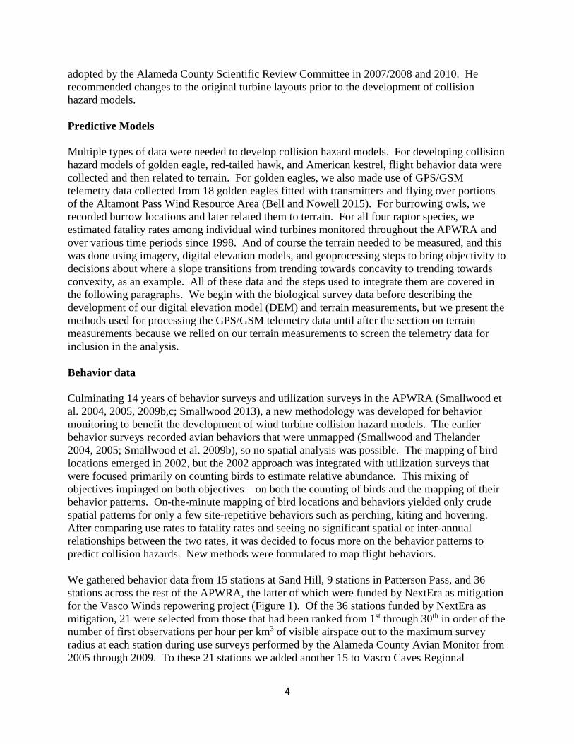
We gathered behavior data from 15 stations at Sand Hill, 9 stations in Patterson Pass, and 36

stations across the rest of the APWRA, the latter of which were funded by NextEra as mitigation

for the Vasco Winds repowering project (Figure 1). Of the 36 stations funded by NextEra as

mitigation, 21 were selected from those that had been ranked from 1st through 30th in order of the

number of first observations per hour per km3 of visible airspace out to the maximum survey

radius at each station during use surveys performed by the Alameda County Avian Monitor from

2005 through 2009. To these 21 stations we added another 15 to Vasco Caves Regional

5

Preserve, Northern Territories, Vasco Winds Energy Project, and the Buena Vista Wind Energy

Project in Contra Costa County, where the Alameda County Avian Monitor had little coverage.

The 15 stations at Sand Hill were optimized to observe how golden eagles and other raptors

behave in the airspace around Ogin’s before-after, control-impact (BACI) experimental

treatment plots designed to test the avian safety of a new wind turbine model that was ultimately

not installed. Seven of the NextEra mitigation stations happened to be located within the

Summit Winds project, and another station was located just outside the project boundary.

Behavior sessions at Sand Hill lasted 30 minutes each, and elsewhere they lasted 1 hour each.

Between 30 April 2012 and 5 March 2015 there were 2,002 surveys completed for 1,001 hours

(126,084 birds tracked). The maximum survey radius depended on the printed map image extent

and how far the observer felt comfortable estimating the bird’s spatial location and height above

ground. Map extents rarely permitted survey distances of >300 m. One of us (Smallwood)

recorded all of the behavior data within Patterson Pass, and additional behavior data were

collected at NextEra mitigation sites by Smallwood, Erika Walther, Elizabeth Leyvas, Skye

Standish, Brian Karas, and Harvey Wilson.

The 9 Patterson Pass stations were surveyed 167 times (167 hours) from 15 October 2013 to 24

September 2014 (5,712 birds tracked). The 36 NextEra mitigation stations were surveyed 928

times (928 hours) from 13 November 2012 through 29 October 2015 (27,552 birds tracked).

Between all three studies, 2,096 hours of behavior surveys (159,348 birds tracked) provided the

data used for developing collision hazard models reported herein.

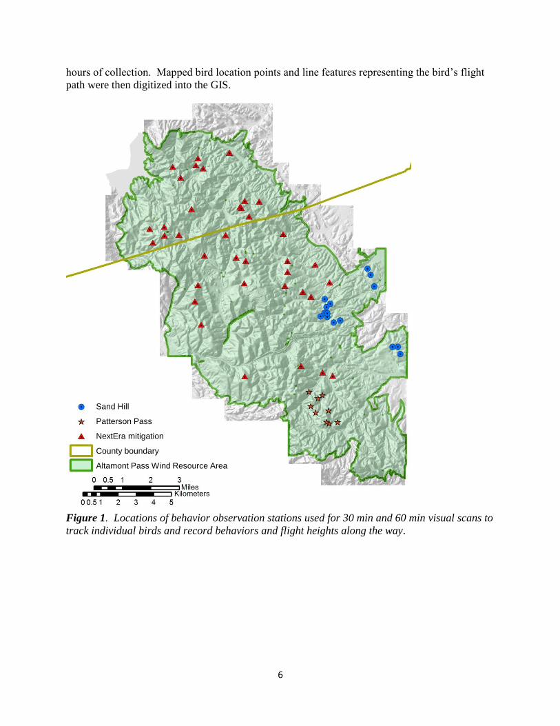
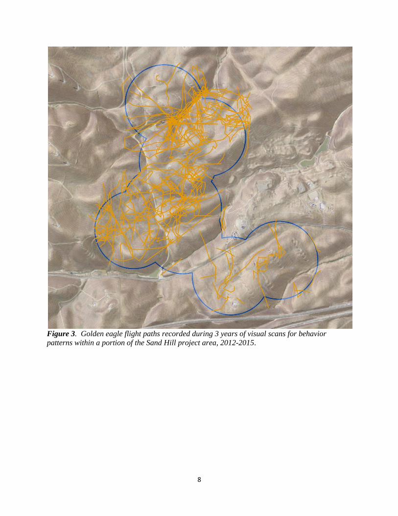
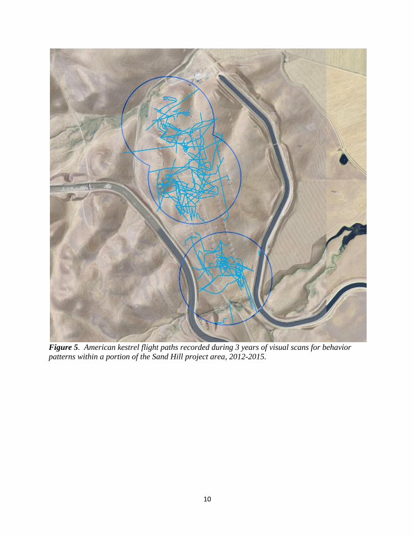
Each bird was recorded onto image-based maps of the survey area as point features connected by

vector lines depicting the bird’s flight path (Figures 2-5). Height above ground, behavior, and

time into the session was recorded into Tascam digital voice recorders fitted with windjammers

designed to reduce noise buffeting by high winds. Point features were recorded as often as the

observer could record attribute data into the voice recorder. One objective of the behavior

sessions was to obtain high quality flight paths and summaries of flight behaviors of individual

birds using the surveyed airspace, and it was notably not to count birds, although it was likely

that just as many raptors were recorded as would have been counted based on the use survey

protocols.

Another objective of the behavior surveys was to learn how birds interact with wind turbines

when they approached the wind turbines. Special attention was given to the bird’s flight

whenever it flew within 50 m of a wind turbine and, in the opinion of the observer, faced the

possibility of colliding with the wind turbine. During this time, the bird’s approach angle to the

turbine was recorded, as well as any changes in flight direction, flight height, behavior,

interactions with other birds, and the wind turbine’s operating status. Whenever special attention

was directed to such flights, the flight observation was termed an “event,” or a wind turbine

interaction event.

At the start of each behavior session, the observer identified which wind turbines in the survey

area were operating, as well as temperature, wind direction, average and maximum wind speed,

and percentage cloud cover. Behavior data were transcribed to electronic spreadsheets within 24

6

hours of collection. Mapped bird location points and line features representing the bird’s flight

path were then digitized into the GIS.

Figure 1. Locations of behavior observation stations used for 30 min and 60 min visual scans to

track individual birds and record behaviors and flight heights along the way.

Sand Hill

Patterson Pass

NextEra mitigation

County boundary

Altamont Pass Wind Resource Area

7

Figure 2. Example of how birds were tracked visually during behavior surveys. Flight attributes

were recorded at points, which were later connected by line segments representing a flight path.

In this case 5 flight paths were recorded, A through E, and at each number associated with a

point we also recorded behavior, height above ground, social group size and, when appropriate,

wind turbine events. For example, D4 would likely have involved a wind turbine event.

8

Figure 3. Golden eagle flight paths recorded during 3 years of visual scans for behavior

patterns within a portion of the Sand Hill project area, 2012-2015.

9

Figure 4. Red-tailed hawk flight paths recorded during 3 years of visual scans for behavior


10

Figure 5. American kestrel flight paths recorded during 3 years of visual scans for behavior


11

Burrowing owl burrows

Burrowing owl burrows (Figure 6) were mapped in sampling plots throughout the APWRA

using a Trimble GeoXT GPS, both during the nesting season (Smallwood et al. 2013) and

throughout the year in 2011 (Figure 7). Additional burrow mapping efforts were made in follow-

up visits during breeding seasons of 2012-2015. Most of the burrows that were mapped were

nest burrows, but refuge burrows were also included in the data pool. No satellite burrows

(alternate nest burrows) were used in the analysis because satellite burrows are merely nearby

extensions of nest burrows.

Figure 6. Example of a burrowing owl nest burrow, including an adult (top) and chicks.

12

Figure 7. Burrowing owl sampling plots (tan color) and 2011 nest and refuge burrow locations

(as examples) within the Altamont Pass Wind Resource Area (blue polygon).

13

Fatality rates

We estimated annual fatality rates at all old generation wind turbines that were searched at least

one year between the years 1998 through 2011 in the APWRA. All fatality rates were adjusted

for search detection and carcass persistence rates that were averaged among wind projects where

trials were performed in similar grassland environments as compared to the APWRA (see

Smallwood 2013). Fatality rates were also adjusted for variation in the maximum search radius

around wind turbines (Smallwood 2013). Finally, we adjusted fatality rates for monitoring

duration to account for a potential bias warned about in Smallwood and Thelander (2004:App.

A). This bias is actually two biases in one, and it applies more to comparing fatality rates among

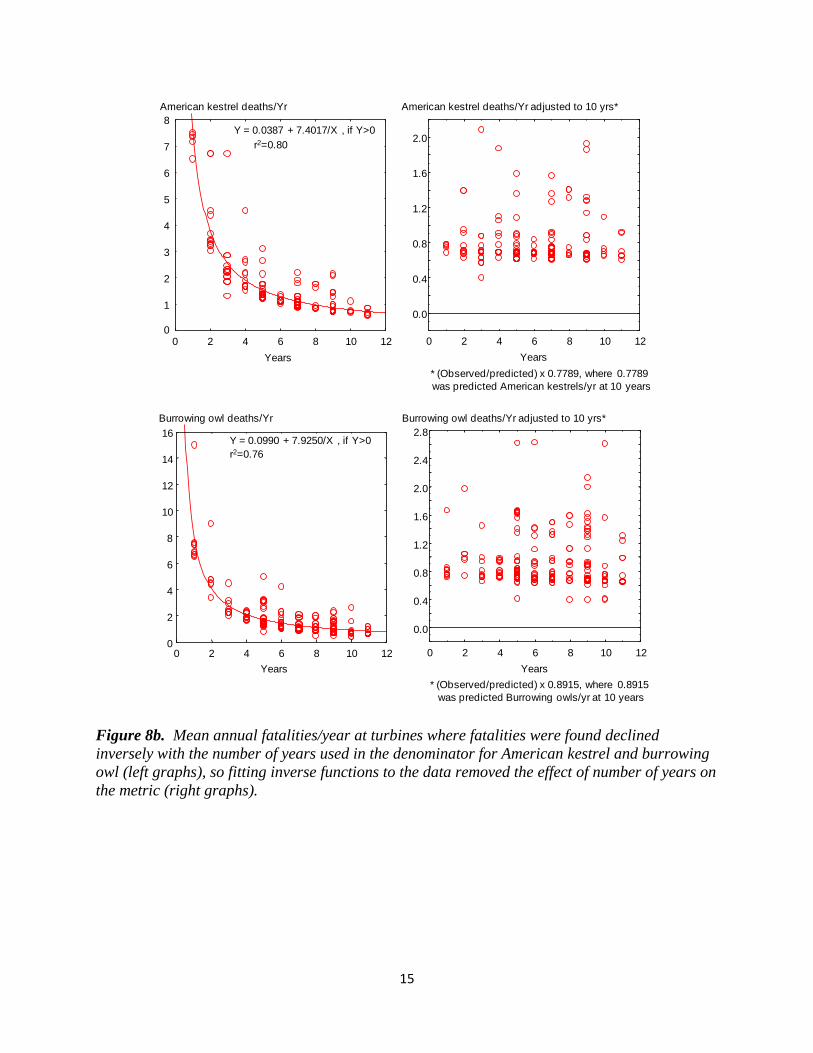
individual wind turbines than it does to wind projects. The adjustments are shown in Figure 8.

Going to the first portion of the bias, as the number of fatalities is averaged into more years of

survey effort, the resulting ratio of fatalities to years will decrease inversely with increasing

number of years for some turbines where fatalities were found, simply because a relatively

constant numerator (number of fatalities) is divided by a constantly changing denominator

(years). If an eagle fatality is found at a wind turbine monitored over one year, the fatality rate

would be 1 eagle death per year, but if this turbine is monitored over 10 years and no more eagle

fatalities are found, then the fatality rate would be 0.1 eagle deaths per year. At a wind turbine

monitored over 10 years, the measured rate should be regarded as reasonably reliable. But a

fatality rate of 1 eagle per year measured at a wind turbine monitored only over 1 year should be

regard as much less reliable because it remains unknown whether additional eagle fatalities

would be found at that turbine had it been monitored over more years. Monitored over 10 years,

this turbine might yield a fatality rate of 1 or more eagle deaths per year or only 0.1 eagle deaths

per year, an uncertainty range of 10-fold or greater.

Going to the second portion of the bias, some fatality rates will represent false zeros where wind

turbines were monitored for only one or a few years and no fatalities were found. Assuming a

golden eagle fatality rate of 0.1 deaths per MW per year and assuming for this example that

fatality risk is equal among 100-KW wind turbines in a project area, then the monitoring duration

sufficient to register a single golden eagle fatality at the average wind turbine would be 100

years. A reasonable assumption would be that false zeroes are common for golden eagle fatality

rate estimates in the APWRA. This bias, or both biases together, was partially corrected by

fitting an inverse function to the data, and then multiplying the ratio of observed to predicted

values by the predicted value at 10 years of monitoring (Figure 8). In other words, all fatality

rates at individual wind turbines were adjusted to a common 10-year period of monitoring, even

if they had been monitored only one year, 4 years, or 10 years, etc. (We note that the fatality rate

metric in this case excluded the turbine’s rated capacity, MW.) Our adjustment reduces the

magnitude of mathematical artefact caused by high fatality rates at wind turbines monitored

briefly, but it does not adjust for false zeroes at wind turbines monitored briefly.

Fatality rates adjusted for duration of monitoring were related to terrain measurements and

terrain features to identify associations useful for developing predictive collision hazard models.

The terrain features and terrain measurements used were those associated with the wind turbines

where fatality rates had been recorded (Figure 9).

14

Figure 8a. Mean annual fatalities/year at turbines where fatalities were found declined

inversely with the number of years used in the denominator for golden eagle and red-tailed hawk

(left graphs), so fitting inverse functions to the data removed the effect of number of years on the

metric (right graphs).

Years

r2=0.64

Y = 0.1050 + 2.7310/X, if Y>0

0 2 4 6 8 10 12

0

1

2

3

4

5

* (Observed/predicted) x 0.3781, where 0.3781

was predicted Red-tailed hawks/yr at 10 years

0 2 4 6 8 10 12

Years

0.0

0.4

0.8

1.2

1.6

2.0

Red-tailed hawk deaths/Yr Red-tailed hawk deaths/Yr adjusted to 10 yrs*


was predicted Golden eagles/yr at 10 years

0 2 4 6 8 10 12

Years

0.1

0.2

0.3

0.4

0.5

0.6

0.7

0.8

0.9

1.0

Years

r2=0.91

Y=0.0647 + 2.5350/X , if Y>0

0 2 4 6 8 10 120.0

0.5

1.0

1.5

2.0

2.5

3.0

Golden eagle deaths/Yr Golden eagle deaths/Yr adjusted to 10 yrs*

15

Figure 8b. Mean annual fatalities/year at turbines where fatalities were found declined

inversely with the number of years used in the denominator for American kestrel and burrowing

owl (left graphs), so fitting inverse functions to the data removed the effect of number of years on

the metric (right graphs).

Years

r2=0.76

Y = 0.0990 + 7.9250/X , if Y>0

0 2 4 6 8 10 120

2

4

6

8

10

12

14

16

Burrowing owl deaths/Yr Burrowing owl deaths/Yr adjusted to 10 yrs*


was predicted Burrowing owls/yr at 10 years

0 2 4 6 8 10 12

Years

0.0

0.4

0.8

1.2

1.6

2.0

2.4

2.8


was predicted American kestrels/yr at 10 years

Years

r2=0.80

Y = 0.0387 + 7.4017/X , if Y>0

0 2 4 6 8 10 120

1

2

3

4

5

6

7

8

0 2 4 6 8 10 12

Years

0.0

0.4

0.8

1.2

1.6

2.0

American kestrel deaths/Yr American kestrel deaths/Yr adjusted to 10 yrs*

16

Figure 9. Golden eagle fatality rates at Altamont Pass wind turbines, 1998 through 2010,

adjusted for the duration of monitoring where gray circles represent monitored wind turbines

where eagle fatalities were not found and colored circles represent adjusted fatality rates from

lowest (yellow) to highest (red).

17

Digital Elevation Model

Two separate digital elevation model (DEM) grids were utilized for this project. The

geoprocessing tasks were performed using a 10 foot cell size DEM created by combining DEMs

obtained from Contra Costa and Alameda Counties. These data sets were produced using

LIDAR data and ARC TIN software by Mapcon Mapping Inc. during 2007-2008. The border of

the APWRA was used as a mask to produce the APWRA DEM composed of 25,440,000 10x10-

foot cells. This DEM was then converted to a cell centroid point feature class and each point

assigned a unique membership number.

All derived parameters were calculated for the entire APWRA DEM and attributed into the cell

centroid point feature class. An aggregated 792-m buffer served as our mask (limit) for

analyzing previously collected bird data against the DEM parameters. The 792-m radius was

converted to a 2,600 foot radius and an additional 200 feet was added to buffer modeling data for

geoprocessing and to ensure that all bird observations would be covered.

The statistical analyses within the APWRA were limited (masked) to data within the areas

searched for raptors within the behavior study areas, for burrowing owl burrows within the

burrowing owl sampling plots, and for fatality rates among the wind turbines that were

monitored at least one year (and the grid cells on which the turbines were located). The resulting

analytical grids within the behavior survey areas were composed of a 7,548,578 (30%) subset of

the 10x10-foot centroid point feature class serving as the study area for the behavior surveys, and

a 393,555 subset serving as the study area for the behavior surveys restricted to 10-m buffered

ridge-like features. These analytical grids were used to develop and test predictive models.

The same geoprocessing steps were used to characterize terrain attributes as reported in

Smallwood and Neher (2010a,b). We used the Curvature function in the Spatial Analysis

extension of ArcGIS 10.2 to calculate the curvature of a surface at each cell centroid. A positive

curvature indicated the cell surface was upwardly convex, a negative curvature indicated the cell

surface was upwardly concave, and zero indicated the cell surface was flat. Curvature data (-51

to 38) were classified using Natural Breaks (Jenks) with 3 classes of curvature – convex, concave

and mid-range. Break values were visually adjusted to minimize the size of the mid-range class.

A series of geoprocessing steps was used, called ‘expand,’ ‘shrink,’ and ‘region group,’ as well

as ‘majority filter tools’ to enhance the primary slope curvature trend of a location. The result

was a surface almost exclusively defined as either convex or concave (expressed as 1 or 0,

respectively, for the variable Curve, and 2 and 1 respectively, for the variable RidgeValley,

which will appear in the models below). Convex surface areas consisted primarily of ridge crests

and peaks, hereafter referred to as ridges, and concave surface areas consisted primarily of

valleys, ravines, ridge saddles and basins, hereafter referred to as valleys.

Line features representing the estimated average centers of ridge crests and valley bottoms were

derived from the following steps. ESRI’s Flow direction function was used to create a flow

direction from each cell to its steepest down-slope neighbor, and then the Flow accumulation

function was used to create a grid of accumulated flow through each cell by accumulating the

weight of all cells flowing into each down-slope cell. A valley started where 50 upslope cells

had contributed to it in the Flow accumulation function, and a ridge started where 55 cells

18

contributed to it. We applied flow direction and flow accumulation functions to ridges by

multiplying the DEM by -2 to reverse the flow. Line features representing ridges and valley

bottoms were derived from ESRI’s gridline and thin functions, which feed a line through the

centers of the cells composing the valley or ridge. Thinning put the line through the centers of

groups of cells ≥40 in the case of valleys. Lines representing ridges and valleys were also

clipped to identify the major valleys and major ridges, or the topographic features dominating the

local skyline and local drainage systems (Figure 10).

Figure 10. Valley bottoms (gold) and ridge crests (blue) for all terrain (top) and major terrain

(bottom) features.

19

We used the two-foot slope analysis grid to create polygons with relatively gentle slope. We

used a Standard Deviation classification to identify areas with < 7.4 % slope. These areas were

then converted to polygons and intersected with the ridge/valley lines to determine polygons

associated with either ridge or valley descriptions. The borders of these polygons were

converted to lines and combined with the ridge/valley line datasets, respectively, and polygons in

valley features were termed valley polygons and polygons on ridge tops were termed ridge

polygons.

Horizontal distances (m) were then measured between each DEM grid cell and the nearest valley

bottom boundary (in the valley line combined data set) and the nearest ridge top boundary or

ridgeline (in the ridgeline combined data set), referred to as distance to valley and distance to

ridge, respectively. These distances were measured from the DEM grid cell to the closest grid

cell of a valley bottom or ridgeline, respectively, not including vertical differences in position.

The total slope distance was the sum of distance to valley and distance to ridge, and expressed

the size of the slope. The DEM grid cell’s position in the slope was also expressed as the ratio of

distance to valley and distance to ridge, referred to as the distance ratio. This expression of the

grid cell’s position on the slope removed the size of the slope as a factor. The same

measurements were made to major valleys and major ridges.

The vertical differences between each DEM grid cell and the nearest valley bottom boundary and

nearest ridge top boundary or ridgeline were referred to as elevation difference, and this measure

also expressed the size of the slope. In addition to the trend in slope grade at each DEM grid

cell, the gross slope was measured as the ratio of elevation difference and total slope distance.

The DEM grid cell’s position on the slope was also expressed as the ratio of the elevation

differences between the grid cell and the nearest valley and between the grid cell and the nearest

ridge, referred to as elevation ratio. Additionally, the grid cell’s position on the slope was

measured as the average of the percentage distance and the percentage elevation to the ridge top.

This mean percentage was named percent up slope, and provided a more robust expression of the

grid cell’s position on the slope (Figure 11). The same measurements were made to major

valleys and major ridges, leading to the variable we named percent up major terrain slope.

Thus, on a small hill adjacent to a major hill in the area, a grid cell could be 90% under percent

up slope and only 30% under percent up major terrain slope.

Percent up slope did not distinguish a grid cell’s position between slopes on large hills versus

medium or small-sized hills, so the local topographic influence of the feature where each cell

was located was expressed by the variable hill size, which was the elevation difference between

the nearest valley bottom polygon and nearest prominent ridge top polygon. Major hill size was

the elevation difference between the nearest major valley bottom and nearest major ridge top.

Breaks in slope were characterized with the ratio of slope to gross slope, and the ratio gross

slope to major gross slope was also calculated. Additional ratios included local to major hill

size, local to major ridge elevation, and local to major valley elevation.

Each DEM grid cell was classified by aspect according to whether it faced north, northeast, east,

southeast, south, southwest, west, northwest, or if it was on flat terrain. Each grid cell was also

20

categorized as to whether its center on the landscape was windward, leeward or perpendicular to

the prevailing southwest and northwest wind directions as recorded during the behavior

observation sessions.

The study area was divided into smaller polygons of land with like aspect, creating a predictor

variable termed Subwatershed Orientation. Existing sub-watershed polygons already had been

created between ridgelines and valley bottom lines. These watershed polygons were further

divided by reviewing the existing 2-foot hypsography (contour) data and then dividing them into

orientation polygons where the overall orientation of the contours changed. An orientation line

feature layer was digitized with a line for each new polygon following the best observed

orientation of that polygon’s contours. Python scripts attributed the new line with its compass

orientation, e.g., N, NNE, NE. These lines were non-directional, so a compass value could be

either the returned value or the direction 180 degrees opposite. These same scripts calculated a

perpendicular compass direction to the returned orientation line direction. The perpendicular

orientation direction had two possible values, differing by 180 degrees based on which side of

the ridge the line described. A reference point within each orientation polygon was

georeferenced by scripts to a generalized aspect grid of the study area. The scripts determined

the correct perpendicular orientation and calculated the compass direction of the orientation

polygon.

Using similar steps, a predictor variable termed Ridge Orientation was created. Ridgelines were

buffered by 10 feet and the resulting ridgeline polygons classified by orientation: north to south,

north-northwest to south-southeast, northwest to southeast, west-northwest to east-southeast,

west to east, west-southwest to east-northeast, southwest to northeast, and south-southwest to

north-northeast. Flight paths crossing ridgelines were related to these Ridge Orientation

polygons in use and availability analysis.

We represented ridgeline slope as the difference between maximum and minimum elevation of

grid cells within buffered ridgelines (as above) divided by the total length of the ridgeline

polygon. We were hoping to characterize the slope of individual ridge features, but our ridgeline

polygons often spanned multiple ridge features, often from one side of a hill across the top to the

other side. Whereas we obtained a crude representation of change in elevation along ridge

features, we did not measure the slope of individual ridge features.

We also derived a variable named ridge context, which was categorized ridge features by their

elevation difference and distance from major ridges (see Figure 10). We subtracted the elevation

of local ridges from the elevation of major ridges and we plotted the elevation differences against

the distances between the local and major ridges. After fitting a regression line to the plot to

isolate the data above the trend line, we rated ridge context as 1 for local ridges at least 790 m

from major ridges, 2 for local ridges between 440 and 790 m distant and at least 40 m lower than

major ridges, 3 for local ridges between 250 and 440 m distant and at least 26 m lower than



major ridges, 6 for local ridges between 25 and 45 m distant and at least 4 m lower than major

ridges or for local ridges between 45 and 75 m distant and at least 6 m lower than major ridges or

for local ridges between 75 and 100 m distant and at least 8 m lower than major ridges. We

21

related adjusted fatality rates to these categories of ridge context to identify disproportionate

fatality rates.

Steps to identify saddles, notches, and benches

Because a large amount of evidence links disproportionate numbers of raptor fatalities to wind

turbines located on aspects of the landscape that are lower than immediately surrounding terrain

or that represent sudden changes in elevation (Figure 12), a special effort was directed toward

identifying ridge saddles, notches in ridges, and benches of slopes. Benches of slopes are where

ridge features emerge from hill slopes that extend above the emerging ridge. These types of

locations are where winds often compress by the landscape to create stronger force, and where

raptors typically cross hilly terrain or spend more time to forage for prey. Compared to

surrounding terrain, these types of features are often relatively flatter or shallower in slope and

sometimes include lower elevations (e.g., saddles). Geoprocessing steps were used to provide

some objectively to the identification of these features, but judgment was also required because

conditions varied widely in how such features were formed and situated (Figure 12).

The same procedures were used as used in the ridge/valley selection. The two foot slope

analysis grid was used to create polygons with a relatively gentle slope. A Standard Deviation

classification was used to identify areas with < 7.4 % slope. These areas were then converted to

polygons. Those polygons not associated with ridge or valley polygons were examined

manually. Where these polygons were visually associated with saddle and or step features, they

were identified as hazard sites representing saddles, notches, or benches. Maps depicting

contours of the variable percent up slope were also examined, because these contours readily

revealed sudden breaks in slope typical of saddles, notches, and benches, which were then also

represented with polygons.

22

Figure 11. Percent up slope across the Altamont Pass Wind Resource Area was derived from

multiple terrain measurements to express a grid cell’s position on the slope regardless of the size

of the slope, where red was at the valley bottoms and dark green at the ridge crests.

23

Figure 12. We delineated polygons where ridge saddles present opportunities for flying birds to

conserve energy by flying through the relatively lower portions of ridge structures (yellow

arrows denote popular flight routes).

GPS/GSM Telemetry

Doug Bell (2015) caught 18 golden eagles using baited traps since 18 December 2012. To each

eagle he affixed 70 g GPS/GSM units manufactured by Cellular Tracking Technologies, LLC

(CTT; http://celltracktech.com/) via backpack harness. CTT units measure 100 mm x 40 mm x

23 mm and run on solar powered batteries during daylight hours (Figure 13). All units recorded

positions at 15 min intervals, and a subset recorded positions at 30 sec intervals during 3 days of

http://celltracktech.com/

24

every month. Actual times between position intervals vary, but are supposed to average 15 min

or 30 sec. CTT Transmitters download data to cell towers daily during prescribed 1 hour

windows, but if a transmitter is beyond cell tower coverage, it will store location data until it

returns to an area with cell coverage. Eagle location data are down-loaded from the CTT

website, and are password protected.

Figure 13. A golden eagle fitted with a GPS/GSM telemetry unit as seen during a visual scan

survey to record behavior patterns.

GPS/GSM telemetry positions were collected from all telemetered golden eagles intersecting the

boundary of the APWRA from the inception of telemetry monitoring through November 2015.

Lines representing flight paths were derived by connecting sequential positions, so each line was

associated with a distance and time interval summed among all line segments, where a line

segment was the line connecting two sequential positions. New flight lines were initiated each

day, as well as when time intervals between sequential positions exceeded 60 sec in the case of

data collected at 30 sec intervals and 1,020 sec in the case of data collected at 15 min (900 sec)

intervals. We also subsampled 15 min interval data from 30 sec data was when the accumulated

time among sequential positions surpassed 900 sec. We included the subsampled 15 min data

with the 15 min interval data.

To assess error in the GPS/GSM telemetry units we placed these units on the ground for long

periods next to a Trimble GeoXT with sub-meter accuracy. We also mounted telemetry units in

the back of Smallwood’s truck (1.2 m above ground) and next to a Trimble GeoXT unit while

driving throughout the APWRA on various dates from 22 October 2014 through 10 September

2015. Our visual examination of the GPS/GSM data indicated high lateral position accuracy

relative to the Trimble GeoXT unit. However, we noticed high vertical error and a large vertical

bias in the GPS/GSM data when examining simple statistics and histograms. Whereas the

Trimble GeoXT unit generated positions that averaged about a meter above the 10-foot DEM

25

surface – where the average was supposed to be – the GPS/GSM data averaged 9 m below the

10-foot DEM surface. We therefore adjusted upward the vertical positions of the telemetered

golden eagles by 9 m. We also generated a cumulative distribution curve of the vertical error in

the truck-mounted telemetry data, and found that 95% of the recorded positions were within 27

m of their true positions above the 10-foot DEM surface (Figure 14). We therefore used 27 m as

a threshold value for determining whether flight lines of golden eagles were above ground.

Flight lines were assigned to the following height domains above our 10-foot DEM: 0 (ground)

was <0 m above the DEM surface, 1 (near ground) = 0 to 27 m above the DEM, 2 (medium)

was >27 m and <200 m above the DEM, and 3 (high) was >=200 m above the DEM.

Figure 14. Cumulative distribution of vertical error measured from 767 GPS/GSM telemetry

positions between two units mounted in the back of Smallwood’s truck at 1.2 m above ground

while driving throughout the APWRA on various dates from 22 October 2014 through 10

September 2015.

Examining data from GPS/GSM transmitters that we maintained at known locations (not affixed

to eagles), we averaged false flight speeds caused by position scatter as 0.3 m/s (1.08 km/hr) for

30 second interval data, and 0.007 m/s (0.026 km/hr) for 15 min interval data. However, relying

on speed alone was often insufficient for determining whether an eagle was flying because

hovering or kiting golden eagles could have remained in the same locations over 30 sec intervals,

and flying golden eagles could have returned to the same positions after flying out and back to

another location or in a circle (these behaviors have been seen during visual surveys many

times).

Whether an eagle was flying was determined as possible (0) if the flight line averaged slower

than the speed of position scatter and ≤0 m above the DEM and intersected 1 subwatershed

polygon, or it averaged slower than the speed of position scatter and <200 m above the DEM and

intersected 1 subwatershed polygon. Whether an eagle was flying was determined as probable

0 10 20 30 40 50 60

Deviation from 0 m above actual height

0.0

0.2

0.4

0.6

0.8

1.0

Proportion of positions of truck-bed telemetry

at 15 min intervals

95% within 27 m

26

(1) it the flight line averaged faster than position scatter and ≤27 m above the DEM and

intersected ≥2 subwatershed polygons, or it averaged ≥3 km/hr and 0-27 m above the DEM and

intersected ≥1 subwatershed polygon, or it averaged ≥1.08 km/hr and 27-200 m above the DEM

and intersected ≥1 subwatershed polygon. Whether an eagle was flying was determined as

certain (2) if the flight line averaged ≥2.5 km/hr or ≥100 m above the 10-foot DEM and

intersected ≥4 subwatershed polygons, or it averaged ≥27 m above the DEM and intersected

≥3subwatershed polygons, or it averaged ≥2.3 km/hr and ≥27 m above the DEM and intersected

≥1subwatershed polygon. To prevent flight lines used in our association analysis from being

falsely generated from position scatter around perched birds, we included lines determined to

have been within height domains 1 or 2 and determined to have been certainly flying (2).

Associations between bird behaviors and terrain attributes

The location of each raptor was characterized by aspect, slope, rate of change in slope, direction

of change in slope, and elevation. These variables were also used to generate raster layers of the

study area, one raster expressing the aspect of the corresponding slope (hereafter referred to as

aspect), and the other expressing whether the landscape feature was tending toward convex

versus concave orientation (expressed in a variable named curve). These features were defined

using geoprocessing.

Fuzzy logic (FL) modeling (Tanaka 1997) was used to predict the likelihood each grid cell

would be used by golden eagle, red-tailed hawk, American kestrel, and burrowing owl. FL

likelihood surfaces were first created by each selected predictor variable. The mean, standard

deviation, and standard error were calculated for each predictor variable among the grid cells

where each targeted bird species was observed during standard observation sessions. These

statistics formed the basis from which FL membership was assigned to grid cells. Depending on

the pattern in the data, FL membership was assigned values of 1 whenever the value of the

predictor variable was within a certain prescribed distance in value from the mean, oftentimes

within 1 SD, but sometimes within 1 or 2 SE. FL membership values of 1 expressed confidence

that grid cells with the corresponding value range for the predictor variable are likely to be

visited by the target species. FL membership values of 0 were assigned to grid cells that were far

from the mean value, usually defined by prescribed distances from the mean such as >2 SD from

the mean. FL membership values of 0 expressed confidence that grid cells with the

corresponding value range for the predictor variable are unlikely to be visited by the target

species. All other grid cells were assigned FL membership values according to the following

formulae, assuming that the likelihood of occurrence of each species will grade gradually rather

than abruptly across grid cells that vary in value of the predictor variable (Y):

0.5 x (1 – cos(π x (Y – Vc) ÷ (Vf – Vc))) below the mean

0.5 x (1 + cos(π x (Y – Vc) ÷ (Vf – Vc))) above the mean,

where Vc represented the variance term (SD or SE) closer to the mean and Vf represented the

variance term farther from the mean.

FL likelihood values were then summed across predictor variables contributing to a species-

specific model. In earlier efforts to develop FL models for golden eagle, red-tailed hawk,

27

American kestrel and burrowing owl in other parts of the APWRA, natural breaks were used to

divide the summed values into 4 classes, but the percentages of study area composing these

classes remained fairly consistent despite use of natural breaks. Therefore, this time the class

divides were established at 63.5%, 83.5%, and 95.5% when natural breaks were not evident;

otherwise, we used natural breaks. Class 1, including FL likelihood values <63.5% (i.e., 63.5%

of the study area), represented the suite of grid cells including fewer bird observations other than

expected. Class 2, including FL likelihood values between 63.5% and 83.5% (i.e., 20% of the

study area), represented the suite of grid cells including about equal or slightly greater than

equal bird observations other than expected. Class 3, including FL likelihood values between

83.5% and 95.5% (i.e., 12% of the study area), represented the suite of grid cells including more

bird observations other than expected. And class 4, including the upper 4.5% of FL likelihood

values, represented the suite of grid cells including substantially more bird observations other

than expected.

The performance of each model was assessed by the magnitude of the ratio of the observed

number to the expected number of observations representing a dependent variable and occurring

within the suite of conditions specified by each FL surface class. Dependent variables included

fatality rates (except for American kestrel), flights <180 m above ground, flights across ridge

features and <180 m above ground (Figure 15), social interactions while flying (Figure 16), wind

turbine interaction events (Figures 17 and 18), and hovering or kiting or surfing behaviors

(Figure 19). FL surface models were later projected across wind project areas.

Figure 15. Example of how golden eagle ridge crossings were quantified. WE buffered flights

within 180 m of the ground by 10 m (purple polygons) and their overlap with 10-m buffered

ridge crests (blue polygons) were counted for each ridge orientation: N-S, NNE-SSW, NE-SW,

ENE-WSW, E-W, ESE-WNW, SE-NW, and SSE-NNW. Colored circles depict golden eagle

fatality rates adjusted for monitoring duration, were red was the highest fatality rates.

28

Figure 16. Social or competitive interactions between flying birds served as a dependent

variable for collision hazard modeling, so associations were sought between interacting birds

and terrain measurements and terrain features.

Figure 17. Wind turbine events of birds adjudged by observers to have flown dangerously close

to wind turbine blades were recorded and used for collision hazard modeling, so associations

were sought between wind turbine events and terrain measurements and terrain features. In this

case a golden eagle narrowly avoided a collision with a moving wind turbine blade.

29

Figure 18. Example of a social interaction between flying golden eagles that also happen to be

near wind turbines. Where and under what conditions these combined social interactions and

wind turbine events occur can assist with predicting collision hazard, but many hours of directed

behavior surveys are needed to accumulate a sufficient number of these events to reliably

associate them with environmental and terrain factors.

Figure 19. Red-tailed hawks kiting near the top of a slope. Red-tailed hawks, American kestrels

and burrowing owls (at night) often perform this behavior just upwind of wind turbines. It is a

known dangerous behavior, having preceded multiple eye-witness accounts of birds drifting with

the wind or being pushed back by wind into operating wind turbine rotors. The behavior is also

dangerous because kiting or hovering birds often break off from these behaviors to glide quickly

with the wind before turning back into the wind to repeat the behaviors over another portion of

the slope, but the glide with the wind often places them in sudden jeopardy of colliding with

turbine blades.

30

Burrowing owl model

Because burrowing owls tend to nest low on the slope, it would be rare for a predictive model of

burrowing owl burrow locations to correspond with terrain where burrowing owls are killed by

wind turbines. Therefore, we developed a burrowing owl fatality model and relied on hazard

classes 3 and 4 of this model wherever the cell centroids were located within 60 m of classes 3 or

4 predicted by the burrow model. Otherwise, all class values of the burrow model remained

unchanged.

RESULTS

GPS/GSM Telemetry of Golden Eagles

All 18 of the golden eagles fitted with GPS/GSM telemetry units intersected the APWRA at

some point during the study (Figure 20). Two of the eagles barely overlapped the APWRA with

3 positions each, so they did not contribute anything to the analysis. Another two eagles

recorded only 15 and 16 positions within the APWRA, so they, too, contributed little if anything

to the analysis. The other 14 eagles contributed hundreds or thousands of positions within the

APWRA.

Our examination of associations between eagle positions and terrain variables indicated no

difference between eagles tracked at 30 sec intervals and those tracked at 15 min intervals.

Therefore, we combined the data from the two position intervals for quantifying associations

with terrain variables. We found high variation in terrain associations between gender and age

classes of eagles, but none of this variation appeared meaningful. However, we noticed strong

differences in terrain associations between the 3 eagles that collided with wind turbines versus

those that have not yet collided with wind turbines. Therefore, we relied mostly on terrain

associations of the 3 eagles that collided with wind turbines to develop a collision hazard model.

After combining data sets based on 30 sec and 15 min intervals, golden eagle telemetry positions

adjusted for vertical bias and intersecting the APWRA numbered 17,025 (14%) at or below

ground (of course, these birds were not truly below ground, but recorded below ground due to

position errors), 79,757 (66%) near ground, 18,396 (15%) within the hazardous height zone of 27

m to 200 m above ground, and 6,079 (5%) high above ground. Of the golden eagle positions

intersecting the APWRA, 1.39% were possibly of flying eagles, 12.88% were probably of flying

eagles, and 85.73% were certainly of flying eagles.

31

Figure 20. GPS/GSM telemetry positions of golden eagles (each color represents a different

eagle) within the boundary of the Altamont Pass Wind Resource Area, December 2012 through

September 2015. Orange lines represent County boundaries, and the blue polygon at the upper

left is Los Vaqueros Reservoir.

Visual Surveys

Behavior surveys performed at Sand Hill through 5 April 2015 numbered 2,002 30-min surveys

and across the rest of the APWRA through 29 October 2015 numbered 1,095 1-hr surveys

elsewhere in the APWRA for a combined 2,096 hours. APWRA-wide observation rates were

0.6115 golden eagles/hour, 1.3597 red-tailed hawks/hour, and 0.4054 American kestrels/hour.

We recorded wind turbine interaction events, including 86 golden eagle events, 156 red-tailed

hawk events, and 98 American kestrel events.

Hazard Models

The FL models of golden eagle were composed of 7 predictor variables based on telemetry data

(Table 1), 3 predictor variables based on behavior data (Table 2), and 9 predictor variables based

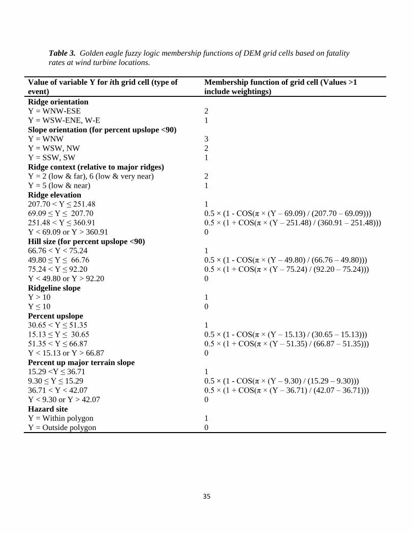
on fatality rates (Table 3). The FL models of red-tailed hawk were composed of 3 predictor

variables based on behavior data (Table 4), and 6 predictor variables based on fatality rates

(Table 5). The FL models of American kestrel were composed of 5 predictor variables based on

behavior data (Table 6), and 7 predictor variables based on fatality rates (Table 7). The FL

models of burrowing owl were composed of 2 predictor variables based on burrow location data

32

(Table 8), and 4 predictor variables based on fatality rates (Table 9). How the models were

weighted and combined for each species is summarized in Table 10.

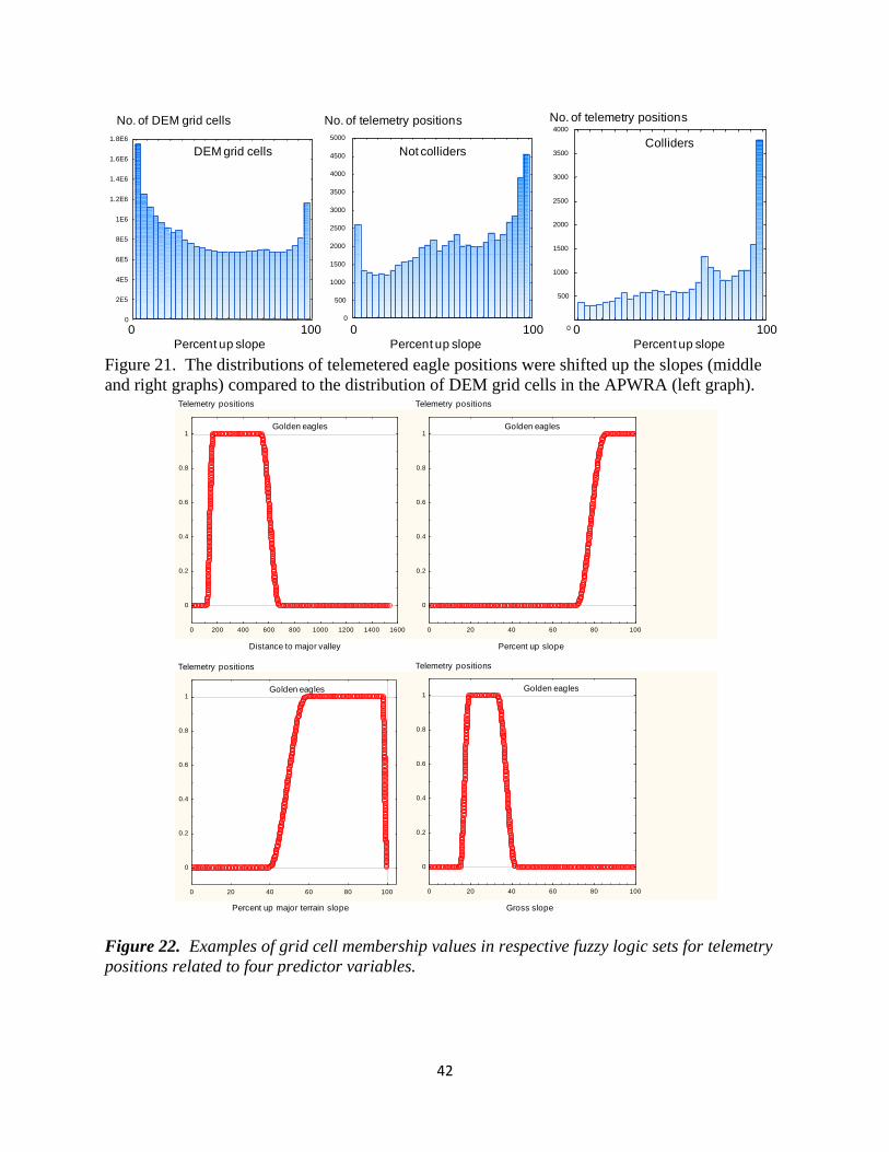
Telemetered golden eagles were recorded flying disproportionately over the upper portions of

slopes, even more so for the colliders (Figure 21). Colliders were also disproportionately

recorded flying higher up the slopes of major terrain features, as well as over ridges oriented east

to west and east-southeast to west-northwest and over slopes facing north-northwest, south-

southwest and south (Figure 22). Colliders were disproportionately recorded flying farther from

the major valley bottoms and over steeper-than-average slopes.

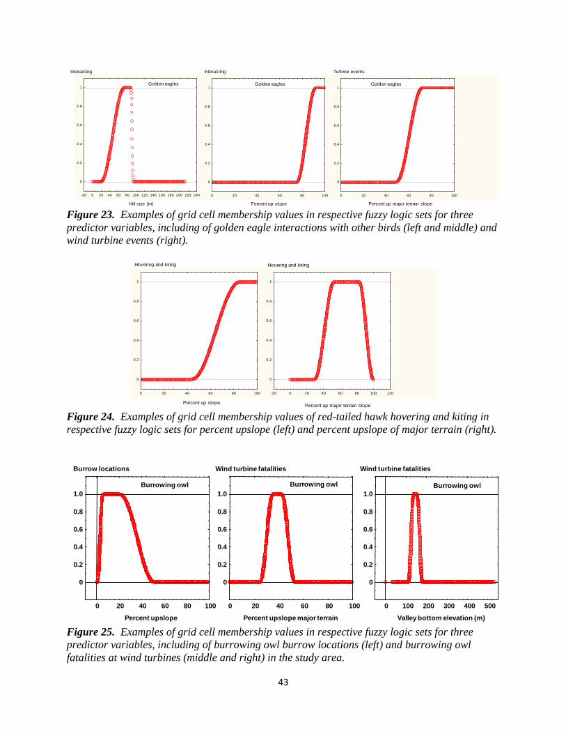
Golden eagle flights and wind turbine interactions occurred disproportionately over ridges

oriented generally west-east. Associations were also strong with subwatershed slopes facing

westerly directions, especially west and northwest. Golden eagles flew and interacted with wind

turbines disproportionately at 91% to 100% up the slope (Figure 23).

Red-tailed hawks hovered and kited disproportionately over slopes oriented north-northeast,

west, and northwest. Red-tailed hawks hovered and kited disproportionately over ground that

was between 85% and 100% to the top of the slope (Figure 24). Red-tailed hawk kiting and

hovering was broader across major terrain features, with peak activity ranging between 53% and

83% to the top of the feature (Figure 24).

American kestrels flew most disproportionately over slopes oriented west and southwest, ranging

mostly between three-quarters to the peak of the slope and midway to just below the peaks of

major terrain features. American kestrel wind turbine interaction events were observed

disproportionately on relatively small hills.

Burrowing owl burrows were located disproportionately between 5% and 30% of the way up

south-facing slopes (Figure 25). Burrowing owl fatality rates were disproportionately higher at

low to moderate elevations and between 35% and 42% of the way up the slopes of major terrain

features and in hazard sites (Figure 25).

Map-based collision hazard models were used to recommend shifts in the initially proposed wind

turbine layout at Summit Winds (Figures 26-29). These models were combined from other

models as described in the Methods section and Table 10. The numbering of proposed wind

turbine sites is provided in the last figure of the Appendix.

33

Table 1. Golden eagle fuzzy logic membership functions of DEM grid cells based on GPS

telemetry positions primarily of 3 study birds that collided with wind turbines.

Value of variable Y for ith grid cell (type of

event)

Membership function of grid cell (Values >1

include weightings)

Ridge orientation

Y = W-E 3

Y = WNW-ESE 2

Y = NW-SE, 1

Y = Other orientation 0

Subwatershed orientation

Y = S, SSW, NNW 2

Y = N, NE, SW, WNW 1


Percent up slope

85.70 < Y ≤ 100 1

71.56 ≤ Y ≤ 85.70 0.5 × (1 - COS(π × (Y – 71.56) / (85.70 – 71.56)))

Y < 71.56 0

Percent up major terrain slope

59.0 < Y ≤ 98.0 1

39.5 ≤ Y ≤ 59.0 0.5 × (1 - COS(π × (Y –39.5) / (59.0 – 39.5)))

98.0 < Y ≤ 100.0 0.5 × (1 + COS(π × (Y –98.0) / (100.0 – 98.0)))

Y < 39.5 0

Distance to major valley

168.81 <Y ≤ 538.34 1

117.25 ≤ Y ≤ 168.81 0.5 × (1 - COS(π × (Y – 117.25) / (168.81 – 117.25)))

538.34 < Y < 684.44 0.5 × (1 + COS(π × (Y – 538.34) / (684.44 – 538.34)))

Y < 117.25 or Y > 684.44 0

Gross slope

19.56 <Y ≤ 33.10 1

15.04 ≤ Y ≤ 19.56 0.5 × (1 - COS(π × (Y – 15.04) / (19.56 – 15.04)))

33.10 < Y < 42.13 0.5 × (1 + COS(π × (Y – 33.10) / (42.13 – 33.10)))

Y < 15.04 or Y > 42.13 0

Hazard site

Y = Within polygon 1

Y = Outside polygon 0

34

Table 2. Golden eagle fuzzy logic membership functions of DEM grid cells based on flights

involving ridge crossings, interactions with other birds, and wind turbine interaction events.


event)


include weightings)

Ridge orientation (ridge crossings, social

interactions, turbine events, behavior)

Y = W-E 2

Y = N-S, NE-SW, WNW-ESE, NNW-SSE 1


Subwatershed orientation (social interactions,

turbine events, behavior)

Y = WSW, W, NW 3

Y = SSE, WNW, SSW, NNW 2

Y = N, NNE, NE, SW 1


Percent up slope (turbine events, social

interactions)

91 < Y ≤ 100 1

15 ≤ Y ≤ 91 0.5 × (1 - COS(π × (Y – 15) / (91 – 15)))

Y < 15 0

35

Table 3. Golden eagle fuzzy logic membership functions of DEM grid cells based on fatality

rates at wind turbine locations.


event)


include weightings)

Ridge orientation

Y = WNW-ESE 2

Y = WSW-ENE, W-E 1

Slope orientation (for percent upslope <90)

Y = WNW 3

Y = WSW, NW 2

Y = SSW, SW 1

Ridge context (relative to major ridges)

Y = 2 (low & far), 6 (low & very near) 2

Y = 5 (low & near) 1

Ridge elevation

207.70 < Y ≤ 251.48 1

69.09 ≤ Y ≤ 207.70 0.5 × (1 - COS(π × (Y – 69.09) / (207.70 – 69.09)))

251.48 < Y ≤ 360.91 0.5 × (1 + COS(π × (Y – 251.48) / (360.91 – 251.48)))

Y < 69.09 or Y > 360.91 0

Hill size (for percent upslope <90)

66.76 < Y < 75.24 1

49.80 ≤ Y ≤ 66.76 0.5 × (1 - COS(π × (Y – 49.80) / (66.76 – 49.80)))

75.24 < Y ≤ 92.20 0.5 × (1 + COS(π × (Y – 75.24) / (92.20 – 75.24)))

Y < 49.80 or Y > 92.20 0

Ridgeline slope

Y > 10 1

Y ≤ 10 0

Percent upslope

30.65 < Y ≤ 51.35 1

15.13 ≤ Y ≤ 30.65 0.5 × (1 - COS(π × (Y – 15.13) / (30.65 – 15.13)))

51.35 < Y ≤ 66.87 0.5 × (1 + COS(π × (Y – 51.35) / (66.87 – 51.35)))

Y < 15.13 or Y > 66.87 0


15.29 <Y ≤ 36.71 1

9.30 ≤ Y ≤ 15.29 0.5 × (1 - COS(π × (Y – 9.30) / (15.29 – 9.30)))

36.71 < Y < 42.07 0.5 × (1 + COS(π × (Y – 36.71) / (42.07 – 36.71)))

Y < 9.30 or Y > 42.07 0

Hazard site



36

Table 4. Red-tailed hawk fuzzy logic membership functions of DEM grid cells based on flights

involving ridge crossings, interactions with other birds, behavior, and wind turbine interaction

events.


event)


include weightings)

Subwatershed orientation (ridge crossings, social interactions, turbine events, hovering/kiting) Y = NNE, W, NW 3

Y = SW, N 2

Y = WSW, WNW, NNW 1


Percent up slope (hovering/kiting)

85.43 < Y ≤ 100 1

43.84 ≤ Y ≤ 85.43 0.5 × (1 - COS(π × (Y – 43.84) / (85.43 – 43.84)))

Y < 43.84 0

Percent up major terrain slope (hovering/kiting)

52.98 < Y ≤ 82.66 1

29.24 ≤ Y ≤ 52.98 0.5 × (1 - COS(π × (Y – 29.24) / (52.98 – 29.24)))

82.66 < Y ≤ 100 0.5 × (1 + COS(π × (Y – 82.66) / (100 – 82.66)))

Y < 29.24 0

37

Table 5. Red-tailed hawk fuzzy logic membership functions of DEM grid cells based on fatality



event)


include weightings)

Ridge orientation

Y = N-S, NW-SE, WNW-ESE, W-E, WSW-ENE 1

Y = NNW-SSE, SW-NE, SSW-NNE 0

Subwatershed orientation (percent upslope <90) Y = SSW, NW 1.5

Y = SW, WNW, NNW 1


Y = 6 (low & very near) 1

Ridge elevation

195.68 < Y ≤ 222.32 1

80.24 ≤ Y ≤ 195.68 0.5 × (1 - COS(π × (Y – 80.24) / (195.68 – 80.24)))

222.32< Y ≤ 320 0.5 × (1 + COS(π × (Y –222.32) / (320 – 222.32)))

Y < 80.24 or Y > 320 0


22.18 <Y ≤ 27.82 1

13.71 ≤ Y ≤ 22.18 0.5 × (1 - COS(π × (Y – 13.71) / (22.18 – 13.71)))

27.82< Y < 36.29 0.5 × (1 + COS(π × (Y – 27.82) / (36.29– 27.82)))

Y < 13.71 or Y > 36.29 0

Hazard site



38

Table 6. American kestrel fuzzy logic membership functions of DEM grid cells based on flights

involving ridge crossings, interactions with other birds, behavior, and wind turbine interaction

events.


event)


include weightings)

Subwatershed orientation (ridge crossings, social interactions, turbine events, hovering/kiting) Y = SE, SSW, SW, W, NNW 3

Y = WSW, NW 2

Y = N, NNE, SSE, S 1


Percent up slope (hovering/kiting)

85.43 < Y ≤ 100 1

43.84 ≤ Y ≤ 85.43 0.5 × (1 - COS(π × (Y – 43.84) / (85.43 – 43.84)))

Y < 43.84 0

Percent up major terrain slope (hovering/kiting)

66.36 < Y ≤ 92.55 1

40.15 ≤ Y ≤ 66.36 0.5 × (1 - COS(π × (Y – 40.15) / (66.36 – 40.15)))

92.55 < Y ≤ 100 0.5 × (1 + COS(π × (Y – 92.55) / (100 – 92.55)))

Y < 40.15

Hill size (turbine events)

20.73 < Y ≤ 25.03 1

9.98 ≤ Y ≤ 20.73 0.5 × (1 - COS(π × (Y – 9.98) / (20.73 – 9.98)))

25.03 < Y ≤ 44.38 0.5 × (1 + COS(π × (Y – 25.03) / (44.38 – 25.03)))

Y < 9.98 or Y > 44.38 0

Hazard site



39

Table 7. American kestrel fuzzy logic membership functions of DEM grid cells based on fatality



event)


include weightings)

Subwatershed orientation Y = NNE, SW 2

Y = SE, SSW 1


Ridge orientation

Y = WSW-ENE 2

Y = NW-SE, NNW-SSE 1


Y = 4 (low & close), 5 (low & near) 1

Valley elevation (percent upslope < 90)

66.75 < Y < 91.25 or 135.88 < Y < 148.12 1

54.50 ≤ Y ≤ 66.75 or 129.75 ≤ Y ≤ 135.88 0.5 × (1 - COS(π × (Y – 54.50) / (66.75 – 54.50)))

0.5 × (1 - COS(π × (Y – 129.75) / (135.88– 129.75)))

91.25 < Y ≤ 103.5 or 148.12 < Y < 154.25 0.5 × (1 + COS(π × (Y – 91.25) / (103.5 – 91.25)))

0.5 × (1 + COS(π × (Y –148.12) / (154.25 – 148.12)))

54.5 < Y > 154.25 0

Slope to gross slope ratio (percent upslope < 90)

0.79 < Y ≤ 1.20 1

0.69 ≤ Y ≤ 0.79 0.5 × (1 - COS(π × (Y – 0.69) / (0.79 – 0.69)))

1.20 < Y ≤ 1.31 0.5 × (1 + COS(π × (Y – 1.2) / (1.31 – 1.2)))

Y < 0.69 or Y > 1.31 0

Distance to major ridge (percent upslope ≥90)

155 < Y ≤ 195 1

75 ≤ Y ≤ 155 0.5 × (1 - COS(π × (Y – 75) / (155 – 75)))

195 < Y ≤ 275 0.5 × (1 + COS(π × (Y – 195) / (275 – 195)))

Y < 75 or Y > 275 0

Hazard site



40

Table 8. Burrowing owl fuzzy logic membership functions of DEM grid cells based on burrow

locations.


event)


include weightings)

Subwatershed orientation

Y = S 2.5

Y = ESE, SE, SSE 1.5

Y = ENE, E 1


Percent up slope

5.56 < Y ≤ 20.83 1

0.47 ≤ Y ≤ 5.56 0.5 × (1 - COS(π × (Y – 0.47) / (5.56 – 0.47)))

20.83 ≤ Y ≤ 51.37 0.5 × (1 + COS(π × (Y – 20.83) / (51.37 – 20.83)))

Y < 0.47 or Y > 51.37 0

Table 9. Burrowing owl fuzzy logic membership functions of DEM grid cells based on fatality



event)


include weightings)

Valley elevation

138.42 < Y ≤ 155.09 1

91.18 ≤ Y ≤ 138.42 0.5 × (1 - COS(π × (Y – 91.18) / (138.42 – 91.18)))

155.09 < Y ≤ 202.32 0.5 × (1 + COS(π × (Y –155.09) / (202.32 – 155.09)))

Y < 91.18 or Y > 202.32 0

Elevation

168.78 < Y ≤ 193.00 1

60.00 ≤ Y ≤ 168.78 0.5 × (1 - COS(π × (Y – 60) / (168.78 – 60)))

193.00 < Y ≤ 440.19 0.5 × (1 + COS(π × (Y –193) / (440.19 – 193)))

Y < 60.00 and Y > 440.19 0


35.51 <Y ≤ 42.85 1

25.05 ≤ Y ≤ 35.51 0.5 × (1 - COS(π × (Y – 25.05) / (35.51 – 25.05)))

42.85 < Y < 52.95 0.5 × (1 + COS(π × (Y – 42.85) / (52.95 – 42.85)))

Y < 25.05 or Y > 52.95 0

Hazard site



41

Table 10. Fuzzy logic models developed for Summit Winds.

Dependent

variable

Model

Max score

possible

Golden eagle

telemetry

Distance to major valley + 2×Percent up slope + 2× Percent up major

terrain slope + Gross slope + 2×Subwatershed orientation + 3×Ridge

orientation + 10×Hazard site

29

Golden eagle

flights

Ridge orientation + 2×Subwatershed orientation + 2×Percent up slope + 10

Golden eagle

fatalities

10×Hazard site + Ridge orientation + 2×Subwatershed orientation +

2×Ridge context + Ridge elevation + 2×Hill size + Ridgeline slope +

Percent upslope + Major terrain upslope

28

Golden eagle

combined

((Telemetry score/29)×2 + Behavior score/10 + (Fatality score/28)×3)/6 1

Red-tailed hawk

kiting

2×(Percent up slope + Percent up major terrain slope) + Subwatershed

orientation

7

Red-tailed hawk

fatalities


Ridge context + Ridge elevation + Percent up major terrain slope

14.5

Red-tailed

hawk

combined

((Behavior score/7) + (Fatality score/14.5))/2 1

American

kestrel kiting


3×Percent up slope + Percent up major terrain slope + Hill size

21

American

kestrel fatalities

8×Hazard site + 2×Ridge orientation + 2×Subwatershed orientation +

2×Ridge context + Valley elevation + Slope to grosslope ratio + Major

ridge distance

21

American

kestrel

combined

((Behavior score/21)×3 + (Fatality score/21))/4 1

Burrowing owl

burrows

2.5×Percent up slope + Subwatershed orientation 3.5

Burrowing owl

fatalities

2×Hazard site + Elevation + 2×Valley elevation + Percent up major

terrain slope

6

42

Figure 21. The distributions of telemetered eagle positions were shifted up the slopes (middle

and right graphs) compared to the distribution of DEM grid cells in the APWRA (left graph).

Figure 22. Examples of grid cell membership values in respective fuzzy logic sets for telemetry

positions related to four predictor variables.

Not colliders

0

2E5

4E5

6E5

8E5

1E6

1.2E6

1.4E6

1.6E6

1.8E6

0

500

1000

1500

2000

2500

3000

3500

4000

4500

5000

0

DEM grid cells

No. of telemetry positions

Colliders

500

1000

1500

2000

2500

3000

3500

4000

No. of telemetry positionsNo. of DEM grid cells

Percent up slopePercent up slope Percent up slope

0 100 0 100 0 100

0 20 40 60 80 100

0.2

0.4

0.6

0.8

0

1


Telemetry positions

Golden eagles

0 20 40 60 80 100

0.2

0.4

0.6

0.8

0

1

Gross slope

Telemetry positions

Golden eagles

0 200 400 600 800 1000 1200 1400 1600

0.2

0.4

0.6

0.8

0

1

0 20 40 60 80 100

0.2

0.4

0.6

0.8

0

1

Percent up slope

Telemetry positions

Golden eagles

Distance to major valley

Telemetry positions

Golden eagles

43

Figure 23. Examples of grid cell membership values in respective fuzzy logic sets for three

predictor variables, including of golden eagle interactions with other birds (left and middle) and

wind turbine events (right).

Figure 24. Examples of grid cell membership values of red-tailed hawk hovering and kiting in

respective fuzzy logic sets for percent upslope (left) and percent upslope of major terrain (right).

Figure 25. Examples of grid cell membership values in respective fuzzy logic sets for three

predictor variables, including of burrowing owl burrow locations (left) and burrowing owl

fatalities at wind turbines (middle and right) in the study area.

-20 0 20 40 60 80 100 120 140 160 180 200 220 240

0.2

0.4

0.6

0.8

0

1

Hill size (m)

Interacting

Golden eagles


Turbine events

0 20 40 60 80 100

0.2

0.4

0.6

0.8

0

1

Percent up slope

Interacting

Golden eagles

0 20 40 60 80 100

0.2

0.4

0.6

0.8

0

1Golden eagles

0 20 40 60 80 100

0.2

0.4

0.6

0.8

0

1

Percent up slope

Hovering and kiting

-20 0 20 40 60 80 100 120

0.2

0.4

0.6

0.8

0

1


Hovering and kiting

20 40 60 80 1000

0.2

0.4

0.6

0.8

0

1.0

0 20 40 60 80 100

0.2

0.4

0.6

0.8

0

1.0

100 200 300 400 5000

0.2

0.4

0.6

0.8

0

1.0

Wind turbine fatalitiesWind turbine fatalitiesBurrow locations

Burrowing owl Burrowing owl Burrowing owl

Valley bottom elevation (m)Percent upslope major terrainPercent upslope

44

Figure 26. Fuzzy Logic likelihood surface classes of golden eagle telemetry, flight behavior and

fatality locations across the Summit Winds project area, Altamont Pass Wind Resources Area,

California, where red corresponds with the highest likelihood of golden eagle collision, orange

corresponds with the second highest likelihood, yellow corresponds with the third highest

likelihood, and dark green corresponds with the least likelihood.

Golden eagle combined

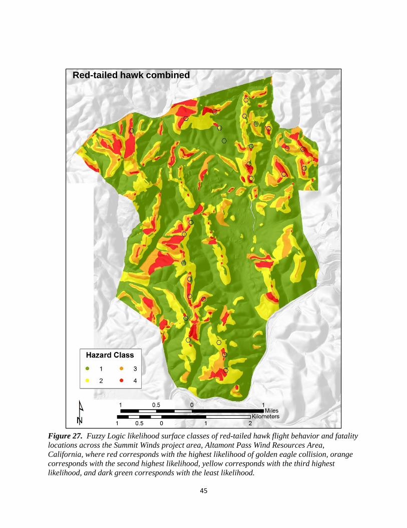
45

Figure 27. Fuzzy Logic likelihood surface classes of red-tailed hawk flight behavior and fatality

locations across the Summit Winds project area, Altamont Pass Wind Resources Area,




Red-tailed hawk combined

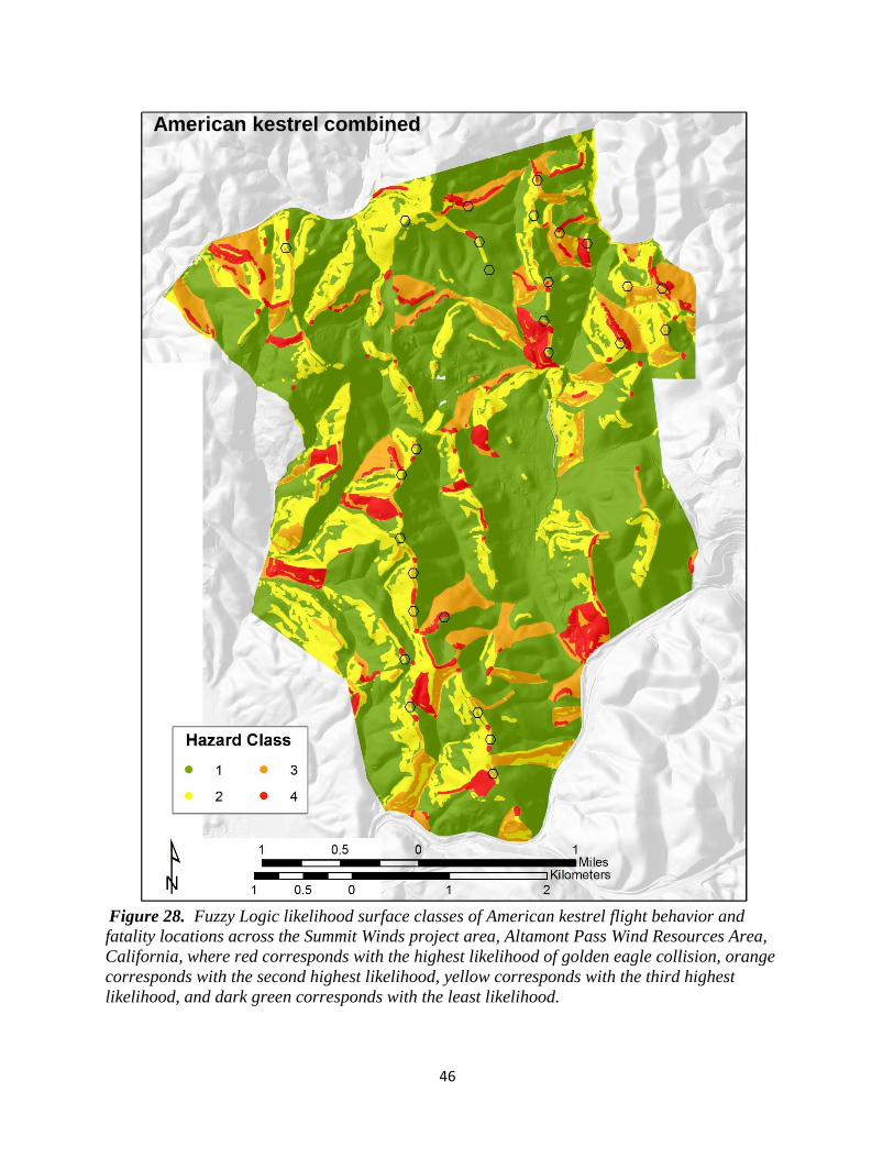
46

Figure 28. Fuzzy Logic likelihood surface classes of American kestrel flight behavior and

fatality locations across the Summit Winds project area, Altamont Pass Wind Resources Area,




American kestrel combined

47

Figure 29. Fuzzy Logic likelihood surface classes of Burrowing owl burrow and fatality

locations across the Summit Winds project area, Altamont Pass Wind Resources Area,

California, where red corresponds with the highest likelihood of burrowing owl collision, orange



Burrowing owl combined

48

DISCUSSION

We produced simple map-based collision hazard models of golden eagle telemetry positions,

ridge crossing flights, wind turbine events, and wind turbine fatalities, as well as of red-tailed

hawk and American kestrel flight behaviors and fatalities in the Altamont Pass Wind Resource

Area. We also produced simple collision hazard models of burrowing owls based on burrow

locations and fatalities at wind turbines. We extended these models to the Summit Winds project

area, which included areas where flight behavior data and burrowing owl burrow data were

collected for developing the collision hazard models. Micro-siting according to these models

and expert opinion should generally achieve the levels of fatality reductions observed at the

repowered Vasco Winds project. After three years of operations at Vasco Winds, and compared

to the old-generation wind project that preceded it, Brown et al. (2016) estimated fatality rate

reductions of 75% to 82% for golden eagle, 34% to 47% for red-tailed hawk, and 48% to 57%

for American kestrel, and 45% to 59% for burrowing owl. However, golden eagle fatality

reductions might be less at Summit Winds due to the constraints of terrain. Some of the

proposed turbine sites are on small hills and ridge structures, leaving little to no room for shifting

turbine locations locally. In these situations, micro-siting is infeasible unless the turbine is

moved to another hill or ridge structure altogether.

Map-based collision hazard maps need to be interpreted carefully, meaning the hazards of

specific terrain and wind situations – ridge saddles, apices of southwest and northwest-facing

concave slopes, and breaks in slope – should always trump model predictions. A few of the

turbine sites that pose little or no conflict with collision hazard classes for golden eagle

nevertheless cause us some concern. For example, we know that golden eagle use is intense

around sites proposed for turbines 5, 8, 9, 10, 11, 13, 17, 18, 19, 28, 31, 32 and 33. Site 17 is

located on the edge of a major travel route used by golden eagles, and site 18 is next to a saddle

and also located upwind of another saddle. Site 8 is atop a slope covered by California

buckeyes, and is used intensively by golden eagles. Site 31 is lower than surrounding terrain and

is often the place where eagles soar to gain lift as they move eastward and upward along the

ridge structure towards site 32; these eagles often launch long-distance glides once they reach a

sufficient altitude from above site 32.

The effects of grading for turbine access roads and tower pads also need to be considered,

because they are not anticipated in the collision hazard models. Changes in the shape of the hills

due to grading can transform the location to a more hazardous situation than was assessed herein.

It would be safer to not enhance ridge saddles or breaks in slope due to grading. It would also be

safer to not leave earthen berms upwind of turbine towers, because doing so decreases the

effective vertical space between the low reach of turbine blades and the ground that birds need to

clear.

Table 11 summarizes the coincidences of proposed wind turbine locations with collision hazard

classes for golden eagle, red-tailed hawk, American kestrel and burrowing owl. Table 11 also

includes some micro-siting recommendations and concerns about proposed sites. Most of the

sites are relatively safe for golden eagles and American kestrels and nearly all sites are relatively

safe for burrowing owls. Slightly less than half the sites are relatively safe for red-tailed hawks.

However, even the relatively safe sites pose some collision risk to these species. Wind turbine

49

sites 3, 11, 14, 19 and 20 are outside hazard classes 3 and 4 for all four focal species. Site 1

could also occur outside hazard classes 3 and 4 for all four species following a small move.

Whereas we focused on four target raptor species, Summit Winds could have adverse impacts on

bats and small birds. We developed no collision hazard maps for bats or small birds. We predict

that small bird fatalities will lessen as a result of the repowering project, because the project will

result in fewer hazardous obstacles on the landscape and airspace will open up for small birds

during migration and resident activities. As for bats, we have no way of predicting the project’s

impacts because we lack sufficient on-site data on fatality rates at old turbines and activity

patterns. Whereas we have data on activity patterns of bats at Summit Winds, we lack enough

data to predict risk or where the risk might be greatest.

In the Appendix we included additional collision hazard maps based on specific types of data. In

response to a request from a member of Alameda County’s Technical Advisory Committee, the

first map depicts golden eagle collision hazard in the absence of fatality data (Figure 30). We

also depict golden eagle collision hazard based on telemetry data (Figure 31), flight behavior

data (Figure 32), fatality data (Figure 33), red-tailed hawk collision hazard based on flight

behavior data (Figure 34) and fatality data (Figure 35), American kestrel collision hazard based

on flight behavior data (Figure 36) and fatality data (Figure 37), and burrowing owl collision

hazard based on burrow locations (Figure 38) and fatality data (Figure 39). All of these maps in

the Appendix are intended as support material and should not be relied upon alone for micro-

siting wind turbines. Figure 40 provides the proposed wind turbine site numbers.

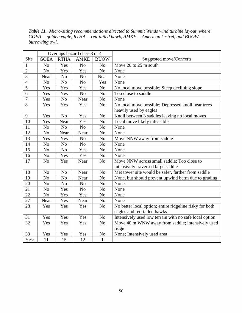
50

Table 11. Micro-siting recommendations directed to Summit Winds wind turbine layout, where

GOEA = golden eagle, RTHA = red-tailed hawk, AMKE = American kestrel, and BUOW =

burrowing owl.

Site

Overlaps hazard class 3 or 4

Suggested move/Concern GOEA RTHA AMKE BUOW

1 No Yes No No Move 20 to 25 m south

2 No Yes Yes No None

3 Near No No Near None

4 No No No Yes None

5 Yes Yes Yes No No local move possible; Steep declining slope

6 Yes Yes No No Too close to saddle

7 Yes No Near No None

8 Yes Yes Yes No No local move possible; Depressed knoll near trees

heavily used by eagles

9 Yes No Yes No Knoll between 3 saddles leaving no local moves

10 Yes Near Yes No Local move likely infeasible

11 No No No No None

12 No Near Near No None

13 Yes Yes No No Move NNW away from saddle

14 No No No No None

15 No No Yes No None


17 No Yes Near No Move NNW across small saddle; Too close to

intensively traversed large saddle

18 No No Near No Met tower site would be safer, farther from saddle

19 No No Near No None, but should prevent upwind berm due to grading

20 No No No No None

21 No Yes No No None


27 Near Yes Near No None

28 Yes Yes Yes No No better local option; entire ridgeline risky for both

eagles and red-tailed hawks

31 Yes Yes Yes No Intensively used low terrain with no safe local option

32 Yes Yes Yes No Move 40 m WNW away from saddle; intensively used

ridge

33 Yes Yes Yes No None; Intensively used area

Yes: 11 15 12 1

51

ACKOWLEDGEMENTS

We thank Salka LLC for the opportunity to develop map-based guidelines for raptor-safe wind

turbine siting. We also thank East Bay Regional Park District, California Energy Commission’s

Public Interest Energy Research program, NextEra Renewables, Ogin Inc. and EDF Renewables

for earlier funding of research that prepared us for this project. Directed behavior surveys were

performed since 2012 by K. S. Smallwood, H. Wilson, E. Walther, B. Karas, J. Mount, S.

Standish, and E. Leyvas. We thank D. Funderburg, S. Michehl, Leah Neher, and S. Neher for

digitizing bird locations from hard-copy maps. We thank D. Bell for use of GPS/GSM telemetry

data of golden eagles.

REFERENCES CITED

Bell, D. A. and C. Nowell. 2015. GPS Satellite Tracking of Golden Eagles (Aquila chrysaetos)

in the Altamont Pass Wind Resource Area (APWRA) and the Diablo Range. Main Report-

Active Birds For the Quarters ending in March and June 2015. Report to Parties to

Repowering Agreement with California Attorney General, Oakland, California.

Brown, K., K. S. Smallwood, J. Szewczak, and B. Karas. 2016. Final 2012-2015 Annual Report

Avian and Bat Monitoring Project Vasco Winds, LLC. Prepared for NextEra Energy

Resources, Livermore, California.

Brown, K., K. S. Smallwood, J. Szewczak, and B. Karas. 2014. Final 2013-2014 Annual Report

Avian and Bat Monitoring Project Vasco Winds, LLC. Prepared for NextEra Energy

Resources, Livermore, California.

Brown, K., K. S. Smallwood, and B. Karas. 2013. Final 2012-2013 Annual Report Avian and

Bat Monitoring Project Vasco Winds, LLC. Prepared for NextEra Energy Resources,

Livermore, California. http://www.altamontsrc.org/alt_doc/p274_ventus_vasco_winds_2012_

13_avian_ bat_monitoring_report_year_1.pdf

ICF International. 2016. Final Report Altamont Pass Wind Resource Area bird fatality study,

monitoring years 2005–2013. Report to Alameda County Community Development Agency,

Hayward, California.

Orloff, S., and A. Flannery. 1992. Wind turbine effects on avian activity, habitat use, and

mortality in Altamont Pass and Solano County Wind Resource Areas: 1989-1991. Report to

California Energy Commission, Sacramento, California.

Smallwood, K. S. 2013. Comparing bird and bat fatality-rate estimates among North American

wind-energy projects. Wildlife Society Bulletin 37: 19-33.

Smallwood, K. S. and C. Thelander. 2004. Developing methods to reduce bird mortality in the

Altamont Pass Wind Resource Area. Final Report to the California Energy Commission,

Public Interest Energy Research – Environmental Area, Contract No. 500-01-019.

Sacramento, California.

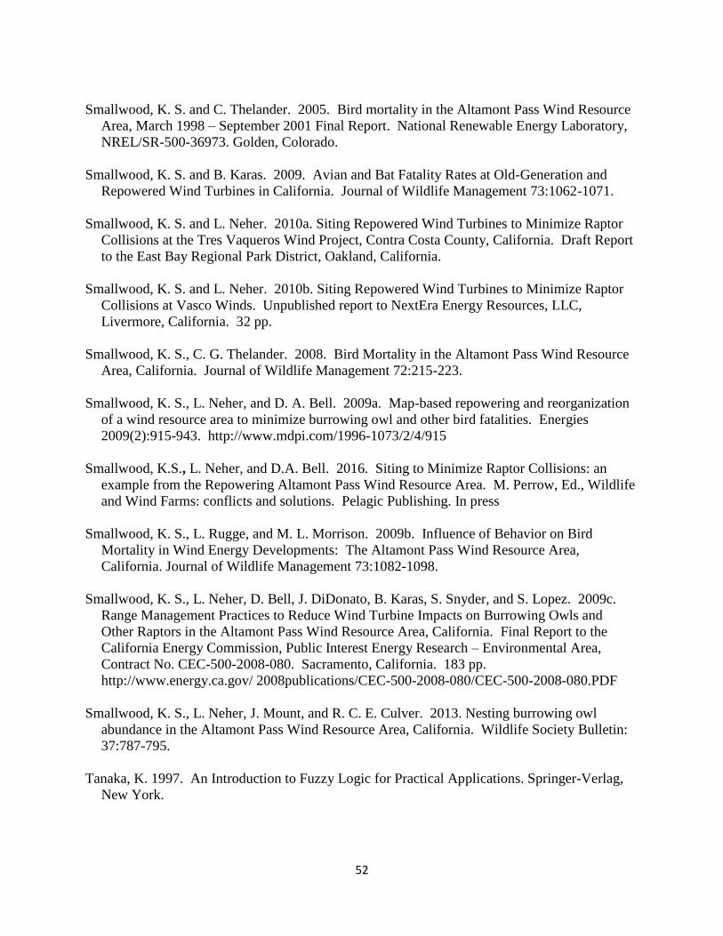
52

Smallwood, K. S. and C. Thelander. 2005. Bird mortality in the Altamont Pass Wind Resource

Area, March 1998 – September 2001 Final Report. National Renewable Energy Laboratory,

NREL/SR-500-36973. Golden, Colorado.

Smallwood, K. S. and B. Karas. 2009. Avian and Bat Fatality Rates at Old-Generation and

Repowered Wind Turbines in California. Journal of Wildlife Management 73:1062-1071.

Smallwood, K. S. and L. Neher. 2010a. Siting Repowered Wind Turbines to Minimize Raptor

Collisions at the Tres Vaqueros Wind Project, Contra Costa County, California. Draft Report

to the East Bay Regional Park District, Oakland, California.

Smallwood, K. S. and L. Neher. 2010b. Siting Repowered Wind Turbines to Minimize Raptor

Collisions at Vasco Winds. Unpublished report to NextEra Energy Resources, LLC,

Livermore, California. 32 pp.

Smallwood, K. S., C. G. Thelander. 2008. Bird Mortality in the Altamont Pass Wind Resource

Area, California. Journal of Wildlife Management 72:215-223.

Smallwood, K. S., L. Neher, and D. A. Bell. 2009a. Map-based repowering and reorganization

of a wind resource area to minimize burrowing owl and other bird fatalities. Energies

2009(2):915-943. http://www.mdpi.com/1996-1073/2/4/915

Smallwood, K.S., L. Neher, and D.A. Bell. 2016. Siting to Minimize Raptor Collisions: an

example from the Repowering Altamont Pass Wind Resource Area. M. Perrow, Ed., Wildlife

and Wind Farms: conflicts and solutions. Pelagic Publishing. In press

Smallwood, K. S., L. Rugge, and M. L. Morrison. 2009b. Influence of Behavior on Bird

Mortality in Wind Energy Developments: The Altamont Pass Wind Resource Area,

California. Journal of Wildlife Management 73:1082-1098.

Smallwood, K. S., L. Neher, D. Bell, J. DiDonato, B. Karas, S. Snyder, and S. Lopez. 2009c.

Range Management Practices to Reduce Wind Turbine Impacts on Burrowing Owls and

Other Raptors in the Altamont Pass Wind Resource Area, California. Final Report to the

California Energy Commission, Public Interest Energy Research – Environmental Area,

Contract No. CEC-500-2008-080. Sacramento, California. 183 pp.

http://www.energy.ca.gov/ 2008publications/CEC-500-2008-080/CEC-500-2008-080.PDF

Smallwood, K. S., L. Neher, J. Mount, and R. C. E. Culver. 2013. Nesting burrowing owl

abundance in the Altamont Pass Wind Resource Area, California. Wildlife Society Bulletin:

37:787-795.

Tanaka, K. 1997. An Introduction to Fuzzy Logic for Practical Applications. Springer-Verlag,

New York.

53

APPENDIX

Figure 30. Fuzzy Logic likelihood surface classes of golden eagle flight behavior and telemetry

data across the Summit Winds project area, Altamont Pass Wind Resources Area, California,

where red corresponds with the highest likelihood of burrowing owl collision, orange



Golden eagle flights & telemetry combined

54

Figure 31. Fuzzy Logic likelihood surface classes of golden eagle telemetry data across the

Summit Winds project area, Altamont Pass Wind Resources Area, California, where red

corresponds with the highest likelihood of burrowing owl collision, orange corresponds with the

second highest likelihood, yellow corresponds with the third highest likelihood, and dark green

corresponds with the least likelihood.

Golden eagle telemetry

55

Figure 32. Fuzzy Logic likelihood surface classes of golden eagle flight behavior data across

the Summit Winds project area, Altamont Pass Wind Resources Area, California, where red




Golden eagle flight behavior

56

Figure 33. Fuzzy Logic likelihood surface classes of golden eagle fatality data across the





Golden eagle fatalities

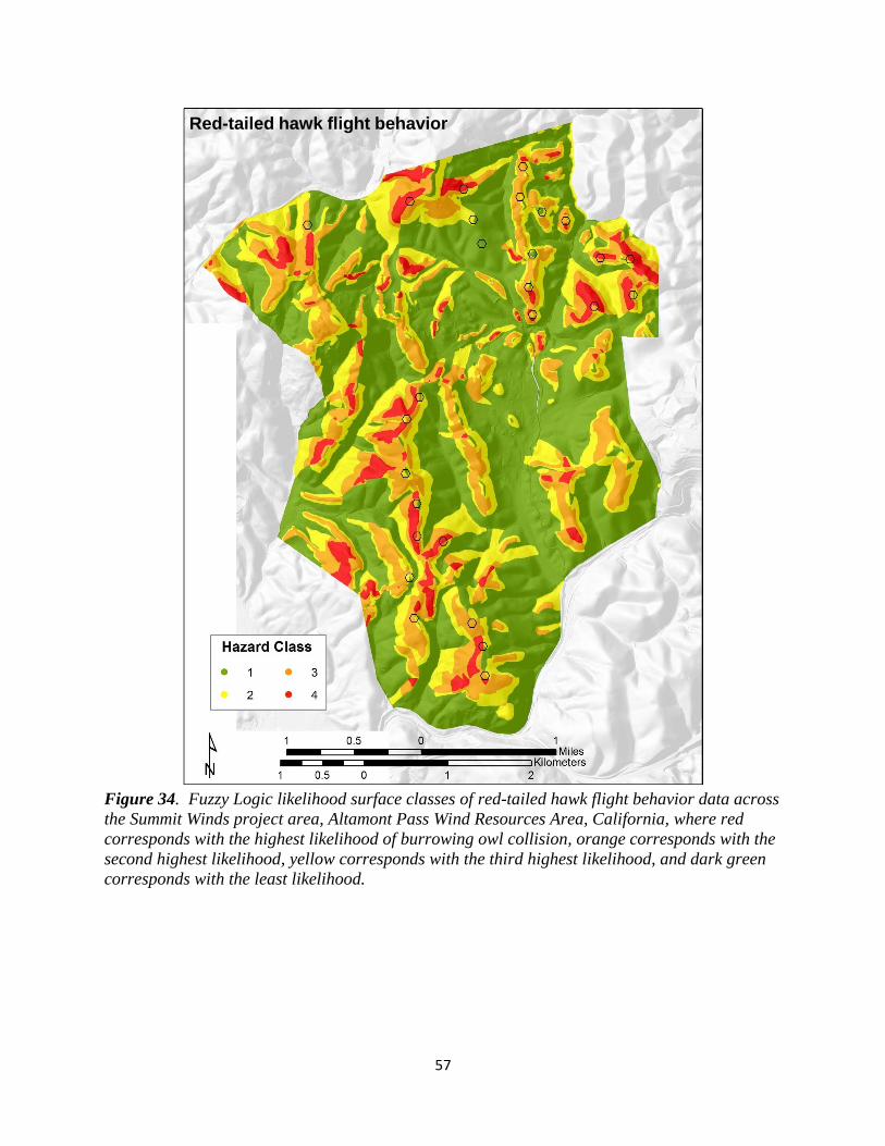
57

Figure 34. Fuzzy Logic likelihood surface classes of red-tailed hawk flight behavior data across

the Summit Winds project area, Altamont Pass Wind Resources Area, California, where red




Red-tailed hawk flight behavior

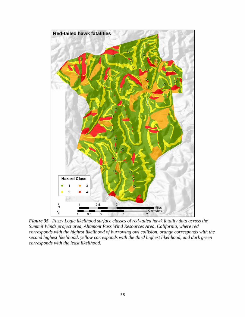
58

Figure 35. Fuzzy Logic likelihood surface classes of red-tailed hawk fatality data across the





Red-tailed hawk fatalities

59

Figure 36. Fuzzy Logic likelihood surface classes of American kestrel flight behavior data

across the Summit Winds project area, Altamont Pass Wind Resources Area, California, where

red corresponds with the highest likelihood of burrowing owl collision, orange corresponds with

the second highest likelihood, yellow corresponds with the third highest likelihood, and dark

green corresponds with the least likelihood.

American kestrel flight behavior

60

Figure 37. Fuzzy Logic likelihood surface classes of American kestrel fatality data across the





American kestrel fatalities

61

Figure 38. Fuzzy Logic likelihood surface classes of burrowing owl burrow locations across the





Burrowing owl burrows

62

Figure 39. Fuzzy Logic likelihood surface classes of burrowing owl fatality locations across the





Burrowing owl fatalities

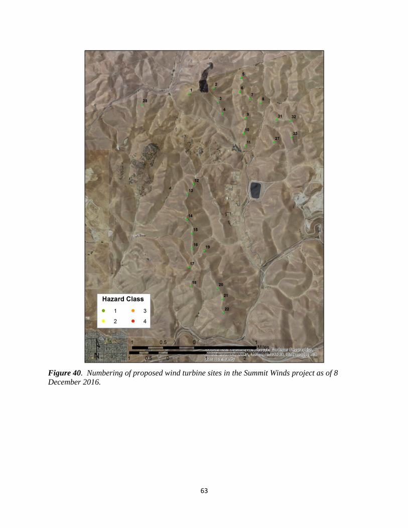
63

Figure 40. Numbering of proposed wind turbine sites in the Summit Winds project as of 8

December 2016.

siting wind turbines to minimize raptor … partly derived from gps/gsm telemetry data transmitted...

Documents