sis digital geometry - institut d'électronique et d...
TRANSCRIPT
UPEM Master 2 Informatique “SIS”
Digital Geometry
Topic 2:Digital topology: object boundaries and
curves/surfaces
Yukiko Kenmochi
October 5, 2016Digital Geometry : Topic 2 1/34
Opening
Representations of discrete shapes
grid point set
graph
(grid points + adjacent relations)
complex
(grid cells + neighboring relations)
Digital Geometry : Topic 2 2/34
Opening
Representations of discrete shapes
grid point set
graph (grid points + adjacent relations)
complex
(grid cells + neighboring relations)
Digital Geometry : Topic 2 2/34

Opening
Representations of discrete shapes
grid point set
graph (grid points + adjacent relations)
complex (grid cells + neighboring relations)
Digital Geometry : Topic 2 2/34
Point set representation
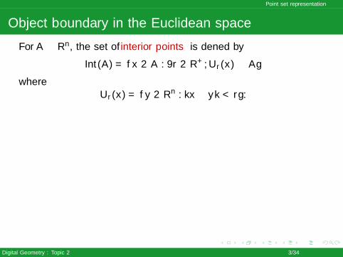
Object boundary in the Euclidean space
For A ⊂ Rn, the set of interior points is defined by
Int(A) = {x ∈ A : ∃r ∈ R+,Ur (x) ⊆ A}where
Ur (x) = {y ∈ Rn : ‖x − y‖ < r}.
The set of border points is:
Br(A) = A \ Int(A).
Then we obtain the set of boundary points such that
Fr(A) = Br(A) ∪ Br(A) = Fr(A).
(Hausdorff, 1937)Digital Geometry : Topic 2 3/34

Point set representation
Object boundary in the Euclidean space
For A ⊂ Rn, the set of interior points is defined by
Int(A) = {x ∈ A : ∃r ∈ R+,Ur (x) ⊆ A}where
Ur (x) = {y ∈ Rn : ‖x − y‖ < r}.The set of border points is:
Br(A) = A \ Int(A).
Then we obtain the set of boundary points such that
Fr(A) = Br(A) ∪ Br(A) = Fr(A).
(Hausdorff, 1937)Digital Geometry : Topic 2 3/34
Point set representation
Object boundary in the nD discrete space
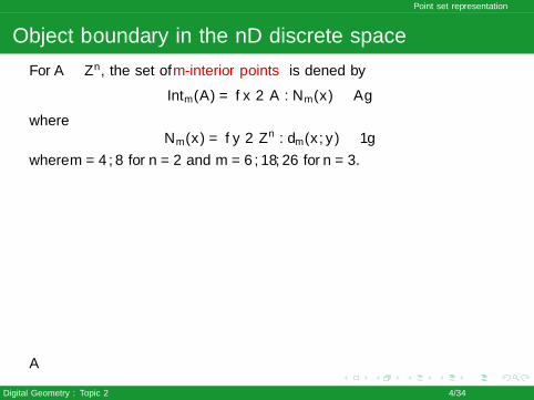
For A ⊂ Zn, the set of m-interior points is defined by
Intm(A) = {x ∈ A : Nm(x) ⊆ A}where
Nm(x) = {y ∈ Zn : dm(x , y) ≤ 1}where m = 4, 8 for n = 2 and m = 6, 18, 26 for n = 3.
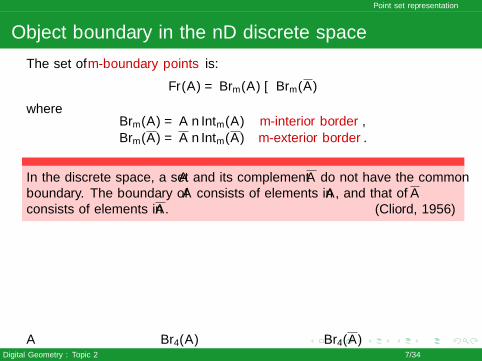
The set of m-boundary points is:
Fr(A) = Brm(A) ∪ Brm(A)
whereBrm(A) = A \ Intm(A) m-interior border,Brm(A) = A \ Intm(A) m-exterior border.
A
Br4(A) Br4(A)
Digital Geometry : Topic 2 4/34
Point set representation
Object boundary in the nD discrete space
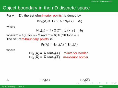
For A ⊂ Zn, the set of m-interior points is defined by
Intm(A) = {x ∈ A : Nm(x) ⊆ A}where
Nm(x) = {y ∈ Zn : dm(x , y) ≤ 1}where m = 4, 8 for n = 2 and m = 6, 18, 26 for n = 3.The set of m-boundary points is:
Fr(A) = Brm(A) ∪ Brm(A)
whereBrm(A) = A \ Intm(A) m-interior border,Brm(A) = A \ Intm(A) m-exterior border.
A Br4(A) Br4(A)
Digital Geometry : Topic 2 4/34
Point set representation
Neighborhoods in the 2D discrete space
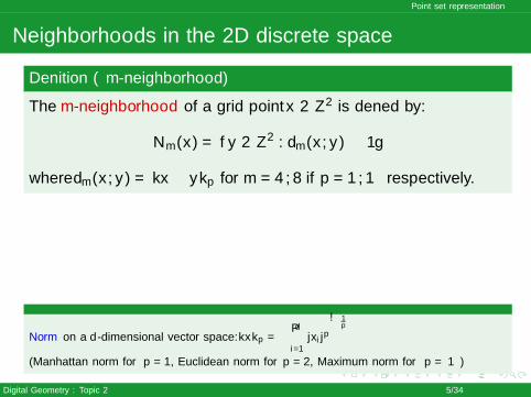
Definition (m-neighborhood)
The m-neighborhood of a grid point x ∈ Z2 is defined by:
Nm(x) = {y ∈ Z2 : dm(x , y) ≤ 1}
where dm(x , y) = ‖x − y‖p for m = 4, 8 if p = 1,∞ respectively.
Norm on a d-dimensional vector space: ‖x‖p =
(d∑
i=1|xi |p
) 1p
(Manhattan norm for p = 1, Euclidean norm for p = 2, Maximum norm for p =∞)
Digital Geometry : Topic 2 5/34
Point set representation
Neighborhoods in the 3D discrete space
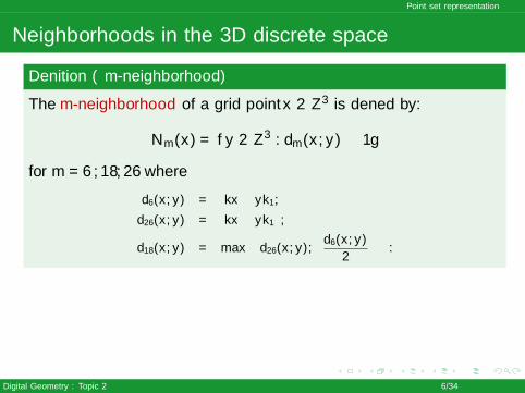
Definition (m-neighborhood)
The m-neighborhood of a grid point x ∈ Z3 is defined by:
Nm(x) = {y ∈ Z3 : dm(x , y) ≤ 1}
for m = 6, 18, 26 where
d6(x , y) = ‖x − y‖1,
d26(x , y) = ‖x − y‖∞,
d18(x , y) = max
{d26(x , y),
⌈d6(x , y)
2
⌉}.
Digital Geometry : Topic 2 6/34
Point set representation
Object boundary in the nD discrete space
The set of m-boundary points is:
Fr(A) = Brm(A) ∪ Brm(A)
whereBrm(A) = A \ Intm(A) m-interior border,Brm(A) = A \ Intm(A) m-exterior border.
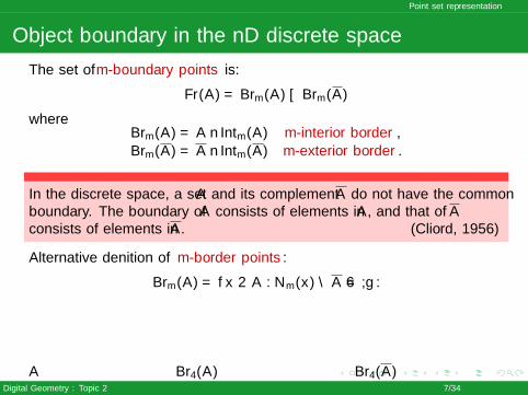
In the discrete space, a set A and its complement A do not have the commonboundary. The boundary of A consists of elements in A, and that of Aconsists of elements in A. (Clifford, 1956)
Alternative definition of m-border points:
Brm(A) = {x ∈ A : Nm(x) ∩ A 6= ∅}.
A Br4(A) Br4(A)Digital Geometry : Topic 2 7/34
Point set representation
Object boundary in the nD discrete space
The set of m-boundary points is:
Fr(A) = Brm(A) ∪ Brm(A)
whereBrm(A) = A \ Intm(A) m-interior border,Brm(A) = A \ Intm(A) m-exterior border.
In the discrete space, a set A and its complement A do not have the commonboundary. The boundary of A consists of elements in A, and that of Aconsists of elements in A. (Clifford, 1956)
Alternative definition of m-border points:
Brm(A) = {x ∈ A : Nm(x) ∩ A 6= ∅}.
A Br4(A) Br4(A)Digital Geometry : Topic 2 7/34
Graph representation
Adjacency graph
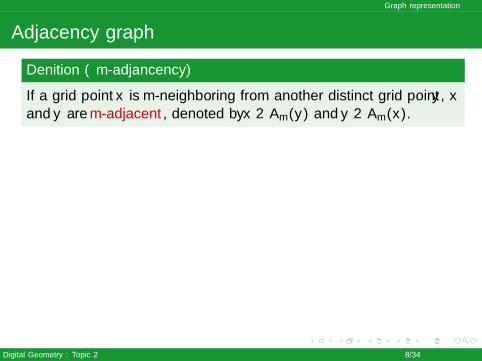
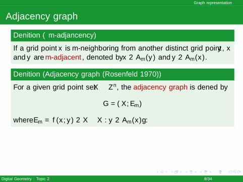
Definition (m-adjancency)
If a grid point x is m-neighboring from another distinct grid point y , xand y are m-adjacent, denoted by x ∈ Am(y) and y ∈ Am(x).
Definition (Adjacency graph (Rosenfeld 1970))
For a given grid point set X ⊆ Zn, the adjacency graph is defined by
G = (X,Em)
where Em = {(x , y) ∈ X× X : y ∈ Am(x)}.
Digital Geometry : Topic 2 8/34
Graph representation
Adjacency graph
Definition (m-adjancency)
If a grid point x is m-neighboring from another distinct grid point y , xand y are m-adjacent, denoted by x ∈ Am(y) and y ∈ Am(x).
Definition (Adjacency graph (Rosenfeld 1970))
For a given grid point set X ⊆ Zn, the adjacency graph is defined by
G = (X,Em)
where Em = {(x , y) ∈ X× X : y ∈ Am(x)}.
Digital Geometry : Topic 2 8/34
Graph representation
Path
Definition (m-Path)
Let X be a set of grid points. An m-path in X joining two points p andq of X is a sequence π = (p0, . . . ,pn) of points in X such thatp0 = p, pn = q and pi ∈ Am(pi−1) for i = 1, . . . , n.
(Klette, Rosenfeld, 2003)
In general, m = 4, 8 for 2D and m = 6, 18, 26 for 3D.
Digital Geometry : Topic 2 9/34
Graph representation
Path
Definition (m-Path)
Let X be a set of grid points. An m-path in X joining two points p andq of X is a sequence π = (p0, . . . ,pn) of points in X such thatp0 = p, pn = q and pi ∈ Am(pi−1) for i = 1, . . . , n.
(Klette, Rosenfeld, 2003)In general, m = 4, 8 for 2D and m = 6, 18, 26 for 3D.
Digital Geometry : Topic 2 9/34

Graph representation
Discrete object (connected component)
Definition (m-object)
A set X of grid points is an m-object if there exists an m-path in X forevery pair p and q of X .
In other words, an m-object is a connected component of a graphG = (X ,Em).
Digital Geometry : Topic 2 10/34

Graph representation
Discrete object (connected component)
Definition (m-object)
A set X of grid points is an m-object if there exists an m-path in X forevery pair p and q of X .
In other words, an m-object is a connected component of a graphG = (X ,Em).
Digital Geometry : Topic 2 10/34

Graph representation
Connected component labeling (of a graph)
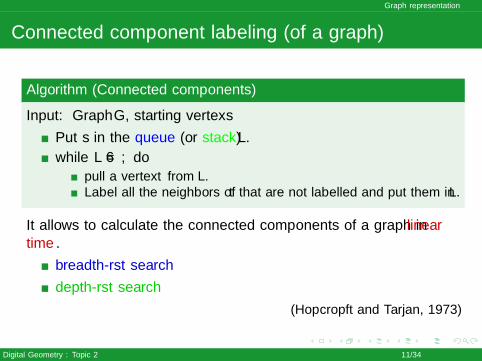
Algorithm (Connected components)
Input: Graph G , starting vertex s
Put s in the queue (or stack) L.
while L 6= ∅ dopull a vertex t from L.Label all the neighbors of t that are not labelled and put them in L.
It allows to calculate the connected components of a graph in lineartime.
breadth-first search
depth-first search
(Hopcropft and Tarjan, 1973)
Digital Geometry : Topic 2 11/34
Graph representation
Connected component labeling (of a graph)
Algorithm (Connected components)
Input: Graph G , starting vertex s
Put s in the queue (or stack) L.
while L 6= ∅ dopull a vertex t from L.Label all the neighbors of t that are not labelled and put them in L.
It allows to calculate the connected components of a graph in lineartime.
breadth-first search
depth-first search
(Hopcropft and Tarjan, 1973)
Digital Geometry : Topic 2 11/34

Graph representation
Discrete curve
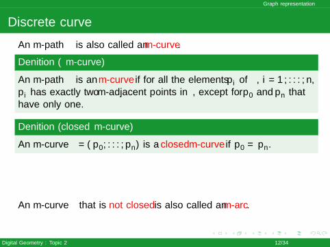
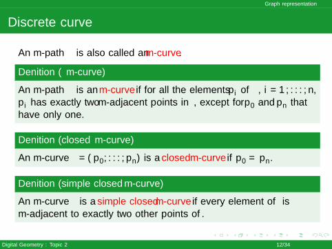
An m-path π is also called an m-curve.
Definition (m-curve)
An m-path π is an m-curve if for all the elements pi of π, i = 1, . . . , n,pi has exactly two m-adjacent points in π, except for p0 and pn thathave only one.
Definition (closed m-curve)
An m-curve π = (p0, . . . ,pn) is a closed m-curve if p0 = pn.
Definition (simple closed m-curve)
An m-curve π is a simple closed m-curve if every element of π ism-adjacent to exactly two other points of π.
Digital Geometry : Topic 2 12/34

Graph representation
Discrete curve
An m-path π is also called an m-curve.
Definition (m-curve)
An m-path π is an m-curve if for all the elements pi of π, i = 1, . . . , n,pi has exactly two m-adjacent points in π, except for p0 and pn thathave only one.
Definition (closed m-curve)
An m-curve π = (p0, . . . ,pn) is a closed m-curve if p0 = pn.
Definition (simple closed m-curve)
An m-curve π is a simple closed m-curve if every element of π ism-adjacent to exactly two other points of π.
Digital Geometry : Topic 2 12/34
Graph representation
Discrete curve
An m-path π is also called an m-curve.
Definition (m-curve)
An m-path π is an m-curve if for all the elements pi of π, i = 1, . . . , n,pi has exactly two m-adjacent points in π, except for p0 and pn thathave only one.
Definition (closed m-curve)
An m-curve π = (p0, . . . ,pn) is a closed m-curve if p0 = pn.
An m-curve π that is not closed is also called an m-arc.
Definition (simple closed m-curve)
An m-curve π is a simple closed m-curve if every element of π ism-adjacent to exactly two other points of π.
Digital Geometry : Topic 2 12/34
Graph representation
Discrete curve
An m-path π is also called an m-curve.
Definition (m-curve)
An m-path π is an m-curve if for all the elements pi of π, i = 1, . . . , n,pi has exactly two m-adjacent points in π, except for p0 and pn thathave only one.
Definition (closed m-curve)
An m-curve π = (p0, . . . ,pn) is a closed m-curve if p0 = pn.
Definition (simple closed m-curve)
An m-curve π is a simple closed m-curve if every element of π ism-adjacent to exactly two other points of π.
Digital Geometry : Topic 2 12/34
Graph representation
Jordan curve theorem
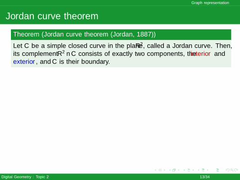
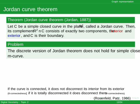
Theorem (Jordan curve theorem (Jordan, 1887))
Let C be a simple closed curve in the plane R2, called a Jordan curve. Then,its complement R2 \ C consists of exactly two components, the interior andexterior, and C is their boundary.
Problem
The discrete version of Jordan theorem does not hold for simple closedm-curve.
If the curve is connected, it does not disconnect its interior from its exterior(8-connectedness); if it is totally disconnected it does disconnect them (4-connectedness).
(Rosenfeld, Pflatz, 1966)
Digital Geometry : Topic 2 13/34
Graph representation
Jordan curve theorem
Theorem (Jordan curve theorem (Jordan, 1887))
Let C be a simple closed curve in the plane R2, called a Jordan curve. Then,its complement R2 \ C consists of exactly two components, the interior andexterior, and C is their boundary.
Problem
The discrete version of Jordan theorem does not hold for simple closedm-curve.
If the curve is connected, it does not disconnect its interior from its exterior(8-connectedness); if it is totally disconnected it does disconnect them (4-connectedness).
(Rosenfeld, Pflatz, 1966)Digital Geometry : Topic 2 13/34
Graph representation
Good adjacency pairs for 2D binary images
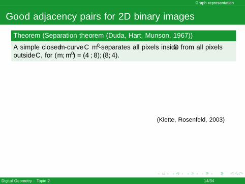
Theorem (Separation theorem (Duda, Hart, Munson, 1967))
A simple closed m-curve C m′-separates all pixels inside C from all pixelsoutside C , for (m,m′) = (4, 8), (8, 4).
(Klette, Rosenfeld, 2003)
Definition (Generarisation: good adjacency pairs (Kong, 2001))
(α, β) is called a good pair iff, for (m,m′) ∈ {(α, β), (β, α)}, any simpleclosed m-curve m′-separates its (at least one) m′-holes from the backgroundand any totally m-disconnected set cannot m′-separate any m′-hole from thebackground.
Digital Geometry : Topic 2 14/34

Graph representation
Good adjacency pairs for 2D binary images
Theorem (Separation theorem (Duda, Hart, Munson, 1967))
A simple closed m-curve C m′-separates all pixels inside C from all pixelsoutside C , for (m,m′) = (4, 8), (8, 4).
(Klette, Rosenfeld, 2003)
Definition (Generarisation: good adjacency pairs (Kong, 2001))
(α, β) is called a good pair iff, for (m,m′) ∈ {(α, β), (β, α)}, any simpleclosed m-curve m′-separates its (at least one) m′-holes from the backgroundand any totally m-disconnected set cannot m′-separate any m′-hole from thebackground.
Digital Geometry : Topic 2 14/34
Graph representation
Exercise: shape border
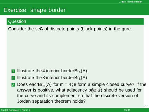
Question
Consider the set A of discrete points (black points) in the figure.
1 Illustrate the 4-interior border Br4(A).
2 Illustrate the 8-interior border Br8(A).
3 Does each Brm(A) for m = 4, 8 form a simple closed curve? If theanswer is positive, what adjacency pair (a, a′) should be used forthe curve and its complement so that the discrete version ofJordan separation theorem holds?
Digital Geometry : Topic 2 15/34
Graph representation
Exercise: shape boundary (answers)
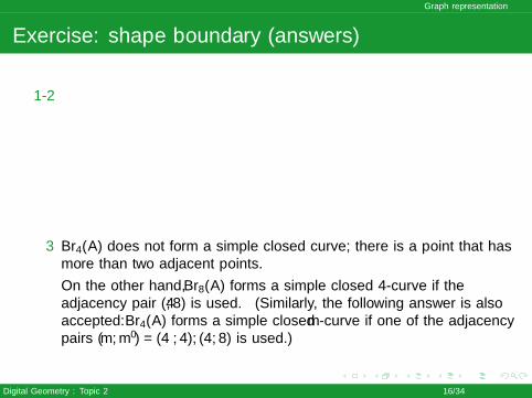
1-2
3 Br4(A) does not form a simple closed curve; there is a point that hasmore than two adjacent points.
On the other hand, Br8(A) forms a simple closed 4-curve if theadjacency pair (4, 8) is used. (Similarly, the following answer is alsoaccepted: Br4(A) forms a simple closed m-curve if one of the adjacencypairs (m,m′) = (4, 4), (4, 8) is used.)
Digital Geometry : Topic 2 16/34
Graph representation
Exercise: shape boundary (answers)
1-2
3 Br4(A) does not form a simple closed curve; there is a point that hasmore than two adjacent points.
On the other hand, Br8(A) forms a simple closed 4-curve if theadjacency pair (4, 8) is used. (Similarly, the following answer is alsoaccepted: Br4(A) forms a simple closed m-curve if one of the adjacencypairs (m,m′) = (4, 4), (4, 8) is used.)
Digital Geometry : Topic 2 16/34

Graph representation
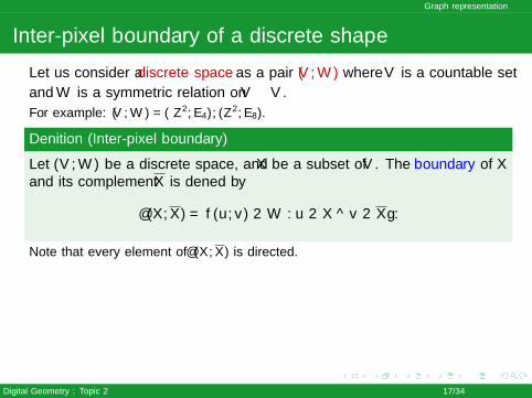
Inter-pixel boundary of a discrete shape
Let us consider a discrete space as a pair (V ,W ) where V is a countable set
and W is a symmetric relation on V × V .
For example: (V ,W ) = (Z2,E4), (Z2,E8).
Definition (Inter-pixel boundary)
Let (V ,W ) be a discrete space, and X be a subset of V . The boundary of Xand its complement X is defined by
∂(X,X) = {(u, v) ∈W : u ∈ X ∧ v ∈ X}.
Note that every element of ∂(X,X) is directed.
(Klette, Rosenfeld, 2003)
Digital Geometry : Topic 2 17/34
Graph representation
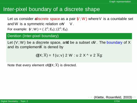
Inter-pixel boundary of a discrete shape
Let us consider a discrete space as a pair (V ,W ) where V is a countable set
and W is a symmetric relation on V × V .
For example: (V ,W ) = (Z2,E4), (Z2,E8).
Definition (Inter-pixel boundary)
Let (V ,W ) be a discrete space, and X be a subset of V . The boundary of Xand its complement X is defined by
∂(X,X) = {(u, v) ∈W : u ∈ X ∧ v ∈ X}.
Note that every element of ∂(X,X) is directed.
(Klette, Rosenfeld, 2003)
Digital Geometry : Topic 2 17/34
Graph representation
Inter-pixel boundary of a discrete shape
Let us consider a discrete space as a pair (V ,W ) where V is a countable set
and W is a symmetric relation on V × V .
For example: (V ,W ) = (Z2,E4), (Z2,E8).
Definition (Inter-pixel boundary)
Let (V ,W ) be a discrete space, and X be a subset of V . The boundary of Xand its complement X is defined by
∂(X,X) = {(u, v) ∈W : u ∈ X ∧ v ∈ X}.
Note that every element of ∂(X,X) is directed.
(Klette, Rosenfeld, 2003)Digital Geometry : Topic 2 17/34
Cell complex approach
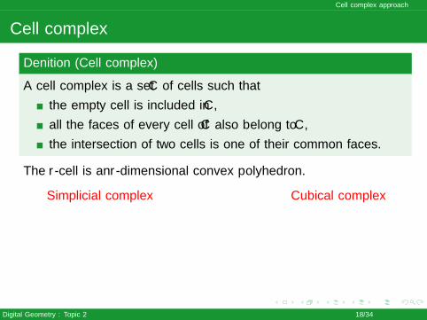
Cell complex
Definition (Cell complex)
A cell complex is a set C of cells such that
the empty cell is included in C ,
all the faces of every cell of C also belong to C ,
the intersection of two cells is one of their common faces.
The r -cell is an r -dimensional convex polyhedron.
Simplicial complex Cubical complex
Digital Geometry : Topic 2 18/34
Cell complex approach
Face of complex
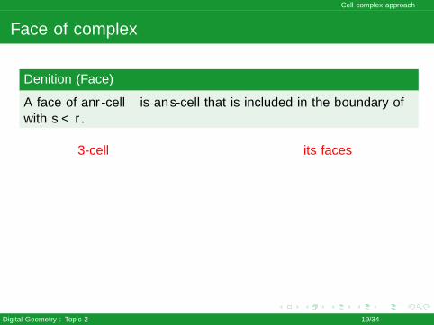
Definition (Face)
A face of an r -cell σ is an s-cell that is included in the boundary of σwith s < r .
3-cell its faces
Digital Geometry : Topic 2 19/34
Cell complex approach
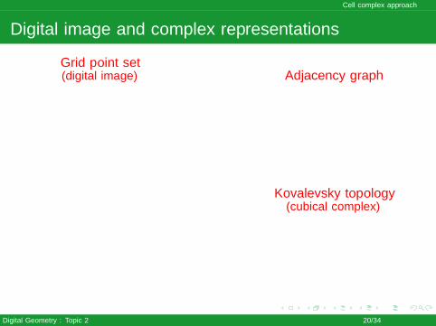
Digital image and complex representations
Grid point set(digital image) Adjacency graph
Kovalevsky topology(cubical complex)
Digital Geometry : Topic 2 20/34
Cell complex approach
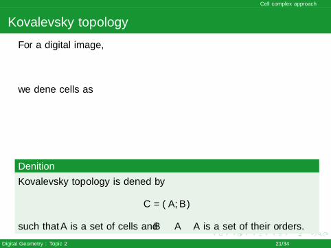
Kovalevsky topology
For a digital image,
we define cells as
Definition
Kovalevsky topology is defined by
C = (A,B)
such that A is a set of cells and B ⊂ A× A is a set of their orders.
Digital Geometry : Topic 2 21/34

Cell complex approach
Order of cells
cell order
If an r -cell σ is a face of s-cell τ , then
σ < τ.
Note: r < s.
Digital Geometry : Topic 2 22/34
Cell complex approach
nD discrete object and boundary (Kovalevsky topology)
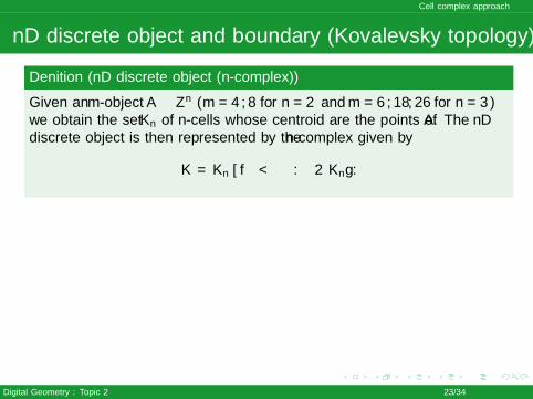
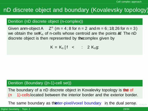
Definition (nD discrete object (n-complex))
Given an m-object A ⊂ Zn (m = 4, 8 for n = 2 and m = 6, 18, 26 for n = 3)we obtain the set Kn of n-cells whose centroid are the points of A. The nDdiscrete object is then represented by the n-complex given by
K = Kn ∪ {τ < σ : σ ∈ Kn}.
Definition (Boundary ((n-1)-cell set))
The boundary of a nD discrete object in Kovalevky topology is the set of(n − 1)-cells located between the interior border and the exterior border.
The same boundary as the inter-pixel/voxel boundary in the dual sense.
Digital Geometry : Topic 2 23/34

Cell complex approach
nD discrete object and boundary (Kovalevsky topology)
Definition (nD discrete object (n-complex))
Given an m-object A ⊂ Zn (m = 4, 8 for n = 2 and m = 6, 18, 26 for n = 3)we obtain the set Kn of n-cells whose centroid are the points of A. The nDdiscrete object is then represented by the n-complex given by
K = Kn ∪ {τ < σ : σ ∈ Kn}.
Definition (Boundary ((n-1)-cell set))
The boundary of a nD discrete object in Kovalevky topology is the set of(n − 1)-cells located between the interior border and the exterior border.
The same boundary as the inter-pixel/voxel boundary in the dual sense.
Digital Geometry : Topic 2 23/34
Cell complex approach
Inter-pixel boundary following
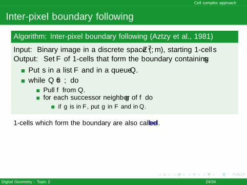
Algorithm: Inter-pixel boundary following (Aztzy et al., 1981)
Input: Binary image in a discrete space (Z 2,m), starting 1-cell sOutput: Set F of 1-cells that form the boundary containing s
Put s in a list F and in a queue Q.
while Q 6= ∅ doPull f from Q.for each successor neighbor g of f do
if g is in F , put g in F and in Q.
1-cells which form the boundary are also called bel.
The graph structure and the similar idea to the graph traversal are used.
Digital Geometry : Topic 2 24/34

Cell complex approach
Inter-pixel boundary following
Algorithm: Inter-pixel boundary following (Aztzy et al., 1981)
Input: Binary image in a discrete space (Z 2,m), starting 1-cell sOutput: Set F of 1-cells that form the boundary containing s
Put s in a list F and in a queue Q.
while Q 6= ∅ doPull f from Q.for each successor neighbor g of f do
if g is in F , put g in F and in Q.
1-cells which form the boundary are also called bel.
The graph structure and the similar idea to the graph traversal are used.
Digital Geometry : Topic 2 24/34
Cell complex approach
Adjacency of 2-cells
Definition (2-cell adjacency)
Given a complex C , two distinct 2-cells of C are adjacent if they havethe common 1-face.
(Lachaud, Malgouyres, 2003)
Property (Voss, 1993)
In the boundary of a 6-object, each 2-cell is adjacent toexactly four neighboring 2-cells such that two of them areits successors and the others are its predecessors.
Digital Geometry : Topic 2 25/34

Cell complex approach
3D boundary following algorithm
Algorithm: 3D boundary following (Aztzy et al., 1981)
Input: 6-object, starting 2-cell sOutput: Set F of 2-cells that form the boundary
Put s in a list F and in a queue Q.
while Q 6= ∅ do
Pull f from Q.for each successor neighbor g of f do
if g is not in F , put g in F and in Q.
(Lachaud, Malgouyres, 2003)
The similar idea to the algorithm for connected component labeling is used.
Digital Geometry : Topic 2 26/34

Cell complex approach
Data structure for Kovalevsky topology
Data structure
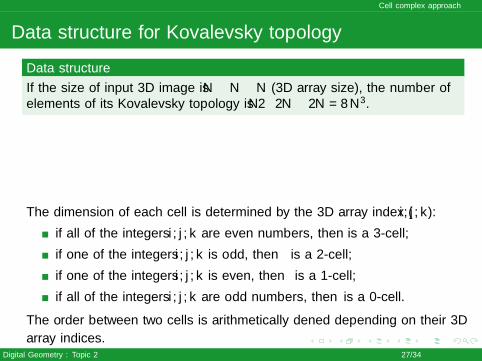
If the size of input 3D image is N × N × N (3D array size), the number ofelements of its Kovalevsky topology is 2N × 2N × 2N = 8N3.
The dimension of each cell σ is determined by the 3D array index (i , j , k):
if all of the integers i , j , k are even numbers, then σ is a 3-cell;
if one of the integers i , j , k is odd, then σ is a 2-cell;
if one of the integers i , j , k is even, then σ is a 1-cell;
if all of the integers i , j , k are odd numbers, then σ is a 0-cell.
The order between two cells is arithmetically defined depending on their 3D
array indices.
Digital Geometry : Topic 2 27/34

Cell complex approach
Data structure for Kovalevsky topology
Data structure
If the size of input 3D image is N × N × N (3D array size), the number ofelements of its Kovalevsky topology is 2N × 2N × 2N = 8N3.
The dimension of each cell σ is determined by the 3D array index (i , j , k):
if all of the integers i , j , k are even numbers, then σ is a 3-cell;
if one of the integers i , j , k is odd, then σ is a 2-cell;
if one of the integers i , j , k is even, then σ is a 1-cell;
if all of the integers i , j , k are odd numbers, then σ is a 0-cell.
The order between two cells is arithmetically defined depending on their 3D
array indices.
Digital Geometry : Topic 2 27/34
Cell complex approach
Data structure for Kovalevsky topology
Data structure
If the size of input 3D image is N × N × N (3D array size), the number ofelements of its Kovalevsky topology is 2N × 2N × 2N = 8N3.
The dimension of each cell σ is determined by the 3D array index (i , j , k):
if all of the integers i , j , k are even numbers, then σ is a 3-cell;
if one of the integers i , j , k is odd, then σ is a 2-cell;
if one of the integers i , j , k is even, then σ is a 1-cell;
if all of the integers i , j , k are odd numbers, then σ is a 0-cell.
The order between two cells is arithmetically defined depending on their 3D
array indices.Digital Geometry : Topic 2 27/34

Cell complex approach
Exercise: connected components and inter-pixel boundary
Question
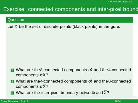
Let X be the set of discrete points (black points) in the figure.
1 What are the 8-connected components of X and the 4-connectedcomponents of X?
2 What are the 4-connected components of X and the 8-connectedcomponents of X?
3 What are the inter-pixel boundary between X and X?
Digital Geometry : Topic 2 28/34

Cell complex approach
Exercise: connected components and inter-pixel boundary
Question
Let X be the set of discrete points (black points) in the figure.
1 What are the 8-connected components of X and the 4-connectedcomponents of X?
2 What are the 4-connected components of X and the 8-connectedcomponents of X?
3 What are the inter-pixel boundary between X and X?
Digital Geometry : Topic 2 28/34
Cell complex approach
Exercise: connected components and inter-pixel boundary
Question
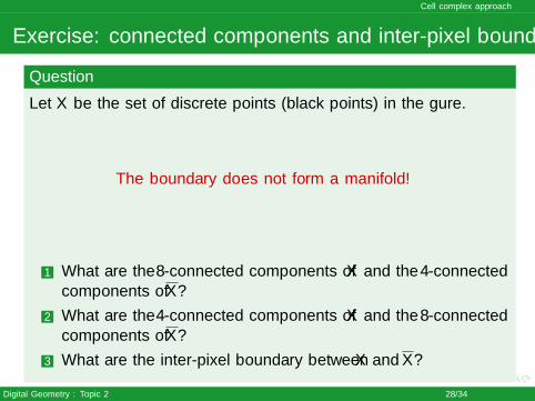
Let X be the set of discrete points (black points) in the figure.
The boundary does not form a manifold!
1 What are the 8-connected components of X and the 4-connectedcomponents of X?
2 What are the 4-connected components of X and the 8-connectedcomponents of X?
3 What are the inter-pixel boundary between X and X?
Digital Geometry : Topic 2 28/34
Well-composed images
Adjacency pair
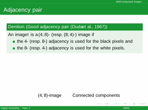
Definition (Good adjacency pair (Duda et al., 1967))
An image I is a (4, 8)- (resp. (8, 4)-) image if
the 4- (resp. 8-) adjacency is used for the black pixels and
the 8- (resp. 4-) adjacency is used for the white pixels.
(4, 8)-image Connected components
Digital Geometry : Topic 2 29/34

Well-composed images
Adjacency pair
Definition (Good adjacency pair (Duda et al., 1967))
An image I is a (4, 8)- (resp. (8, 4)-) image if
the 4- (resp. 8-) adjacency is used for the black pixels and
the 8- (resp. 4-) adjacency is used for the white pixels.
(8, 4)-image Connected components
Digital Geometry : Topic 2 29/34

Well-composed images
Well-composed image
Definition (Well-composed image (Latecki, 1998))
An image is well-composed if each 8-connected component for theblack (and white) points is also a 4-connected component.
Well-composed image 8-connected components
Digital Geometry : Topic 2 30/34
Well-composed images
Well-composed image
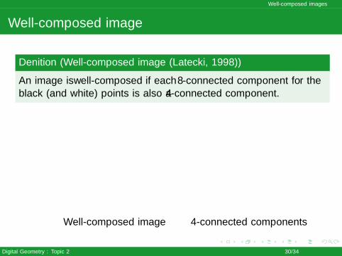
Definition (Well-composed image (Latecki, 1998))
An image is well-composed if each 8-connected component for theblack (and white) points is also a 4-connected component.
Well-composed image 4-connected components
Digital Geometry : Topic 2 30/34

Well-composed images
Well-composed image
Definition (Well-composed image (Latecki, 1998))
An image is well-composed if each 8-connected component for theblack (and white) points is also a 4-connected component.
Ill-composed image 8-connected components
Digital Geometry : Topic 2 30/34
Well-composed images
Well-composed image
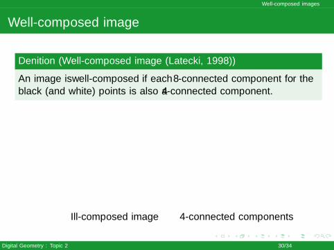
Definition (Well-composed image (Latecki, 1998))
An image is well-composed if each 8-connected component for theblack (and white) points is also a 4-connected component.
Ill-composed image 4-connected components
Digital Geometry : Topic 2 30/34

Well-composed images
Properties of well-composed images
Property (Well-composed image (Latecki, 1998))
Any well-composed image
is characterized by 2× 2 local configuration, and
has no topological paradox related to Jordan Theorem.
Ill-composed image 4-connected components
Digital Geometry : Topic 2 31/34
Well-composed images
Properties of well-composed images
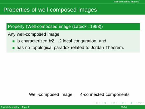
Property (Well-composed image (Latecki, 1998))
Any well-composed image
is characterized by 2× 2 local configuration, and
has no topological paradox related to Jordan Theorem.
Well-composed image 4-connected components
Digital Geometry : Topic 2 31/34

Well-composed images
Repairing images to be well-composed
If a given image is not well-composed, it can be repaired.(Latecki, 1998; Rosenfeld et al., 1998)
Iterative method: modify every critical configuration iterativelysuch that the well-composedness is satisfied.
Up-sampling method: increase the resolution and repair eachcritical configuration locally.
Digital Geometry : Topic 2 32/34
Well-composed images
Repairing images to be well-composed
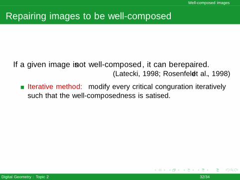
If a given image is not well-composed, it can be repaired.(Latecki, 1998; Rosenfeld et al., 1998)
Iterative method: modify every critical configuration iterativelysuch that the well-composedness is satisfied.
Up-sampling method: increase the resolution and repair eachcritical configuration locally.
Digital Geometry : Topic 2 32/34

Well-composed images
Repairing images to be well-composed
If a given image is not well-composed, it can be repaired.(Latecki, 1998; Rosenfeld et al., 1998)
Iterative method: modify every critical configuration iterativelysuch that the well-composedness is satisfied.
Up-sampling method: increase the resolution and repair eachcritical configuration locally.
Digital Geometry : Topic 2 32/34

Summary
Summary
nD discrete object boundary is expected to be
a Jordan curve/surface,
a n-manifold.
For this aim, we need to choose appropriate shape representations,such as inter-pixel boundary, with
”good” adjacency pair, or
verifying if a given image is well-composed.
Digital Geometry : Topic 2 33/34

Summary
Summary
nD discrete object boundary is expected to be
a Jordan curve/surface,
a n-manifold.
For this aim, we need to choose appropriate shape representations,such as inter-pixel boundary, with
”good” adjacency pair, or
verifying if a given image is well-composed.
Digital Geometry : Topic 2 33/34
References
References
Reinhard Klette and Azriel Rosenfeld.Chapters 4 and 7 in ”Digital geometry: geometric methods fordigital picture analysis”, San Diego: Morgan Kaufmann, 2004.
David Coeurjolly, Annick Montanvert, et Jean-Marc Chassery.”Elements de base”, Chapitre 1 dans ”Geometrie discrete etimages numeriques”, Hermes Lavoisier, 2007.
Jacques-Olivier Lachaud et Remy Malgouyres.”Topologie, courves et surfaces discretes”, Chapitre 3 dans”Geometrie discrete et images numeriques”, Hermes Lavoisier,2007.
Gabor T. Herman.”Geometry of digital spaces”, Birkhauser, 1998.
Longin Jan Latecki.”Discrete representation of spatial objects in computer vision”,Kluwer Academic Publishers, 1998.
Digital Geometry : Topic 2 34/34