�

�

�

�

�

��

���������������� � ���������������������� ����� ������������ ����� ��� ��� ������ � �����

�Timo Sipiläinen Almas Heshmati

June 2004

DP 2004/3

��

���������������� � ���������������������� ����� ������������ ����� ��� ��� ������ � �����

Timo Sipiläinen and Almas Heshmati

MTT Economic Research Luutnantintie 13

FIN-00410 Helsinki Finland

�� +358-9-56086221 �� +358-9-5631164

�. timo.sipilainen@mtt.fi and almas.heshmati@mtt.fi

June 11, 2004

���������

The objective is to examine sources of productivity change on Finnish dairy farms in the 1990s. The decomposition of productivity change into technical change and technical efficiency change is widely recognized but it neglects the price and scale effects. The generalized decompositions incorporating all four components are calculated in a sample of Finnish dairy farms for 1989-2000. The period is of interest because of the drastic change in agricultural policy when Finland joined the European Union (EU) in 1995. The results show that productivity growth has been on average low, approximately 1% per year. Technical change is identified to be the most important source of productivity growth. Technical efficiency change does not vary systematically over time. The role of scale is also minor in productivity change. Cumulative price effects are small but considerable price distortions could be observed at the time of EU accession. In the detailed analysis of efficiency, the extended Kolmogorov-Smirnov tests of first and second order stochastic dominance in distribution of inefficiency were employed. Partial control for time and many farm-specific attributes, such as size, location and production factor intensities by comparing group cells were offered. A number of strong second order rankings between groups was found.

��������� ��� ����������� C14; C23; D24; L25; Q12

�������� Malmquist index; technical efficiency; technical change; scale effect; price effect; SFA; stochastic dominance, bootstrap, inefficiency distribution, testing. ______________________________________________________________________ ��!!������ � ��� ��� Sipiläinen, T. & Heshmati, A. 2004. Sources of Productivity Growth and Stochastic Dominance Analysis of Distribution of Efficiency. MTT Economic Research, Agrifood Research Finland. Discussion Papers 2004/3.

1

1. Introduction In measuring productivity, a ratio between output(s) and input(s) is computed. In the case of single output and single input, this is trivial but when the number of inputs and outputs increases, a method of aggregation is needed to compute productivity. In the latter case, we could employ some index numbers like the Fisher (1922) ideal or Törnqvist (1936) superlative productivity indices (see Diewert and Nakamura 2003 for a detailed discussion). Both of these indices require price and quantity data but no modelling and estimation are needed. In addition, assumptions about technology and behaviour of the decision-maker have to be made. Indices like the Fisher and Törnqvist indices can be used to show whether the quantity index of outputs changes at a different rate compared to the quantity index of inputs, i.e. to show the rate of productivity change. The problem is that we cannot separate the sources of productivity change in these indices (Kumbhakar and Lovell 2000).

Productivity measures may encompass several components the identification and quantification of which are crucial to different economic decision makings. If we assume constant returns to scale and efficiency of production, productivity growth equals technical change, i.e. the shift of production frontier (or production function). Technical change over time is realized as improvements in output-input relationship. In practice, it is possible that there exists increasing economies of scale1 such that proportional increase in output is more than corresponding proportional changes in inputs. Thus, technical change and the increase in farm size may be related. Technical change may also be biased towards some inputs so that the share of certain inputs (e.g. capital) increases compared to others (e.g. labour) over time. Output bias is also possible. In this case technical change, effects the efficient allocation of inputs and outputs.

If we allow for technical inefficiency (and constant returns to scale) but assume allocative efficiency, then productivity growth equals the change in technical efficiency multiplied by the rate of technical change (Nishimizu and Page 1981). By the term technical efficiency, we follow Farrell’s (1957) definition of technical efficiency.2 If we allow for allocative inefficiency, the farm may be technically efficient lying on the isoquant but it is not producing the output by minimum cost (or producing maximum revenue by given inputs). Inefficiency in allocation of inputs effects the cost shares (return shares) which are often utilized in the aggregation of inputs and outputs to construct the quantity indices.

In principle, we can decompose the productivity change to four components: technical change, technical efficiency change, scale effect and price (allocative) effect.

In the case of several inputs and outputs, it is possible to apply the Malmquist productivity index (1953) to measure total factor productivity. The Malmquist index serves also our purpose in identifying various sources of productivity change since

1 If we are talking about economies of size, the minimum cost combination of inputs is dependent on

the size of operation. 2 Efficiency is measured the ratio between observed and potential output using the best practice

technology as reference. The ratio indicates possible equiproportional increase in outputs keeping inputs constant or equiproportional decrease in inputs keeping outputs constant by using frontier technology.

2

several decompositions for this index have been proposed (Färe et al. 1994, Orea 2002, Lovell 2003). This index has the advantage that it does not require price information or behavioural assumptions, however a representation of the production technology is needed in the form of distance functions, which is applicable to cases with multiple inputs and outputs. In case of only single output (or input), the analysis is similar to production function analysis. The index can be calculated or estimated using nonparametric or econometric techniques3. The distance function applications were at first almost entirely based on nonparametric data envelopment analysis (DEA) models. Recently several authors have developed parametric counterparts for those distance functions (see e.g. Coelli et al. 1999 and Brümmer et al. 2002 and references there).

The advantage of the nonparametric techniques is the minimum requirements needed about the technology for the calculation of distance functions but on the other hand, only an econometric approach may allow for stochastic circumstances affecting production and productivity. On the other hand, econometric techniques require assumptions to be made about the functional form, which despite limited testing possibilities may not be correctly chosen.

In earlier Finnish studies of productivity change, both econometric estimation (Hemilä 1982, Ylätalo 1987, Ryhänen 1994, Sipiläinen and Ryhänen 2002) and index numbers (Ihamuotila 1972, Sims 1994, Myyrä and Pietola 1999) have been applied. The majority of these studies is relatively old. One exception is Myyrä’s and Pietola’s (1999) research in which they used data covering almost the entire 1990s and applying index number techniques. Sipiläinen (2003) has studied the productivity growth on dairy and cereal farms applying nonparametric methods and the Malmquist index. No recent research on Finnish data has been conducted applying up-to-date econometric techniques on productivity and efficiency analysis.

The 1990s are a period of interest since Finland joined the European Union (EU) in the middle of the decade. When Finland became a member in the EU at the beginning of 1995, there followed a fundamental change in national agricultural policy, resulting in drastically lower output prices as well as somewhat lower input prices.4 The immediate threat of a corresponding fall in agricultural income was softened by an increase in direct payments. A five-year transition period with decreasing support and a range of investment subsidies were applied to help farmers adjust to the changes following on EU membership. In addition, prior to membership, several restrictions on agricultural production were already introduced. Therefore, an evaluation of the effects of EU membership and restrictions imposed on agricultural production is highly desirable.

The aim of this paper is to investigate the sources of productivity change by decomposing the Malmquist productivity index. This paper provides a detailed analysis of productivity changes for a sample of specialized Finnish dairy farms in the 1990s. We present a decomposition, which can recognize all essential productivity change

3 Important links between index number and econometric estimation techniques have been shown to

exist. For instance, Nadiri (1970) showed that the underlying function for the Laspeyres total factor productivity (TFP) index is constant elasticity of substitution (CES) production function. Diewert (1976) also showed that the Törnqvist total factor productivity (TFP) index is exact for a linearly homogeneous translog function. Later, Diewert (1992) states that Fisher TFP index (geometric mean of Laspeyres and Paasche index) is exact for a flexible variable profit function.

4 The cereal and beef prices were cut to half and even more.

3

effects like technical change (both neutral and non-neutral) and technical efficiency change, but also price effects. The latter may be important in restrictive production conditions (milk quotas, set-aside, etc.) and in cases of considerable regime changes (EU accession). Technical efficiency changes and factors affecting technical efficiency are also carefully tested. The efficiency is estimated both when data is measured per farm and per cow levels. We employ the extended Kolmogorov-Smirnov tests of first and second order stochastic dominance in distribution of inefficiency by controlling for the time period and several farm-specific attributes. This allows for the statistical comparison of the whole distribution rather than points of inefficiency.

The structure of the paper is the following. First, in Section 2, we present the concept of productivity, in general, and the Malmquist productivity index, in particular, and introduce different ways to decompose the index. Then, we show how these indices can be calculated applying parametric distance functions. The data is described in Section 3. Empirical specification of the parametric distance function is outlined in Section 4. In Section 5, we discuss results from identification of the sources of productivity and the decomposition of the productivity index. The analysis of dominance in the distribution of inefficiency by various farm attributes is discussed. The final Section concludes.

2. The Methodology

In this paper, we apply econometric methods for measurement and analysis of total factor productivity (TFP). Let’s assume that the production technology can be presented using output set Y(x), which defines the set of output vectors My R+∈ that can be produced by an input vector Nx R+∈ . That is MY(x) {y R : x can produce y}+= ∈ . The output distance function can be defined as OD (x, y) min{ : y / Y(x)}= θ θ ∈ . DO(x,y) is non-decreasing, positively linearly homogenous and convex in y, and decreasing in x. The value of the distance function is less than or equal to one for all feasible output vectors. On the outer boundary of the production possibilities set, the value of DO(x,y) is one. Thus, the output distance function indicates the potential radial expansion of production to the frontier. Stochastic frontier production function analysis can be extended to stochastic output distance function analysis if there are several outputs. Assuming a translog specification and technical change represented by a time trend, it can be written as (Coelli et al. 1999, Fuentes et al. 2001):

(1)

ph h ht t t t t t tO i i 0 k ki kj ki ji m mi

k 1 k j 1 m 1

p p ph ht t t t 2 t

mn mi ni km ki mi t tt kt kim n 1 k 1 m 1 k 1

pt

mt mim 1

1ln D (x , y ) ln x ln x ln x ln y2

1 1ln y ln y ln x ln y t t ln x t2 2

ln y t

= ≤ = =

≤ = = = =

=

= β + β + β + β

+ β + β + β + β + β

+ β

� �� �

�� �� �

�

where x:s are inputs, y:s outputs, t is time, β :s are coefficients to be estimated and DO is the output distance function. The symmetry of coefficients is also assumed.

It is not possible to estimate the function in (1) in its current form unless the property of linear homogeneity in outputs is applied. The output distance function is by definition

4

linearly homogenous in outputs. Dividing the outputs by one of the outputs imposes the linear homogeneity in outputs. This follows by the following constraints:

(2) 1 1 1 1

1; 0; 0 0p p p p

m mn km mtm m m m

andβ β β β= = = =

= = = =� � � �

Homogeneity in output implies that:

(3) ( , / ) ( , ) /t t t t t t t tO i i mi O i i miD x y y D x y y=

Transforming the variables in logarithms and rearranging the equation gives the translog functional form (TL is an abbreviation):

(4) ln ( , / , ; ) ln ( , )t t t t t t tmi i i mi O i iy TL x y y t D x yβ− = − .

Setting tit O it itu ln D (x , y )= and adding a stochastic error term, our presentation is similar

to that of a parametric stochastic frontier with a decomposed error term:

(5) ln ( , / , ; )t t t tmi i i mi it ity TL x y y t u vβ− = + +

where itu are time-varying inefficiency effects. The estimated parameters can now be used to construct the output oriented Malmquist productivity index for each production unit in the analysis.

At early stages of development of the productivity analysis methodology, productivity change was considered identical with technological change. Technological change describes how the sets of feasible input-output combinations expand or contract. Later on, technical efficiency change has been invented as an important factor in productivity growth. When technological change is related to shifts of the frontier, efficiency change shows if the firm is getting closer to or further away from the frontier. The use of the Malmquist index enables us to combine these changes. However, according to Balk (2001, p. 160) there remain two problems: first, whether to use actual or artificial technology and secondly, how to take scale effect (scale efficiency) into account. The scale of production may affect the productivity (in the sense of output-input relation), and thus also the productivity changes, even if the firm operates on the frontier but in a different scale (or size). Therefore, we define also scale effect as a part of productivity change.

In addition to changes in levels of inputs and outputs, in a multiple input multiple output case, input and output mixes may change over time. These changes may also affect productivity change. In this regards e.g. Kumbhakar and Lovell (2000) emphasize that also price or market effects should be taken into account when TFP changes are evaluated.

In order to measure productivity change, time has to be incorporated. Let's denote t and t+1 two adjacent periods. Thus, t t tD (x , y ) refers to the evaluation of the firm's distance in the period t from the frontier of the same period. When evaluated against the technology of the period t, the Malmquist productivity index is:

(6) t t 1 t 1

tt t t

D (x , y )M

D (x , y )

+ +

=

5

but, when evaluated against the technology of the period t+1 it is written as:

(7) t 1 t 1 t 1

t 1t 1 t t

D (x , y )M

D (x , y )

+ + ++

+= .

However, the choice of the time period is arbitrary. Caves et al. (1982) presented that under the assumption of technical and allocative efficiency (s.t. translog functional form) productivity change is equal to a geometric mean of these two indices:

(8)

1t t 1 t 1 t 1 t 1 t 1 2

t t t t 1 t t

D (x , y ) D (x , y )M

D (x , y ) D (x , y )

+ + + + +

+

� �= � �� �

.

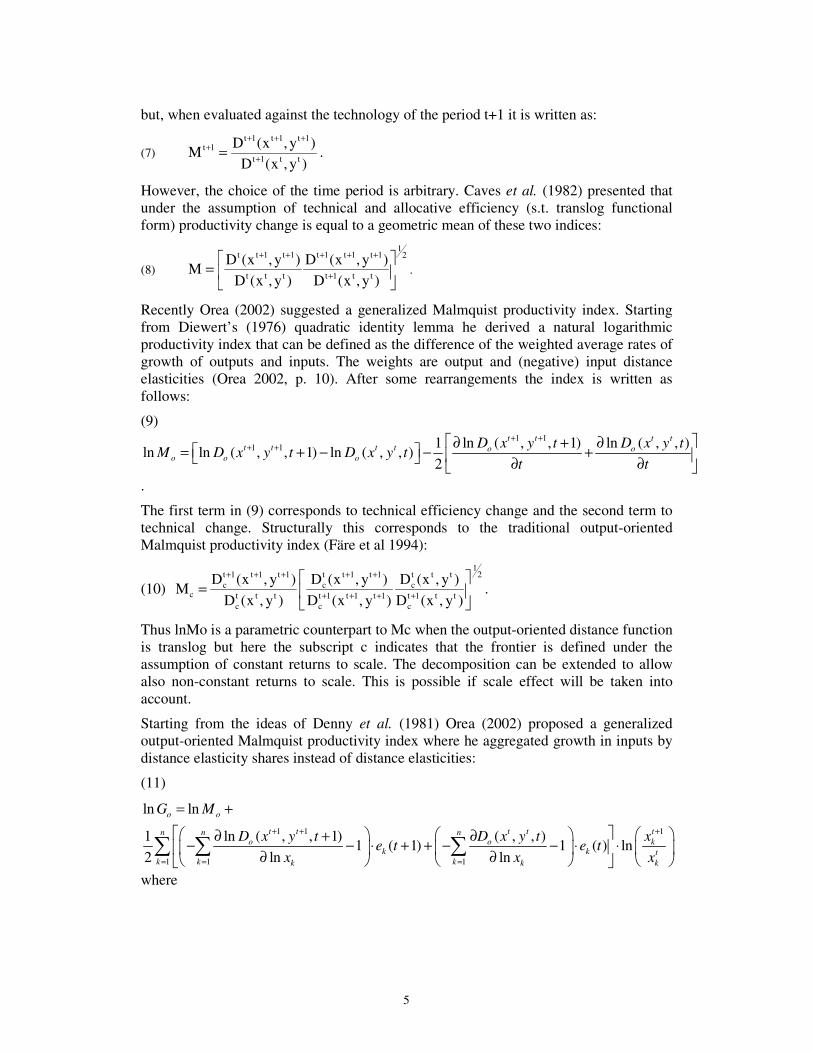
Recently Orea (2002) suggested a generalized Malmquist productivity index. Starting from Diewert’s (1976) quadratic identity lemma he derived a natural logarithmic productivity index that can be defined as the difference of the weighted average rates of growth of outputs and inputs. The weights are output and (negative) input distance elasticities (Orea 2002, p. 10). After some rearrangements the index is written as follows:

(9)1 1

1 1 ln ( , , 1) ln ( , , )1ln ln ( , , 1) ln ( , , )

2

t t t tt t t t o o

o o o

D x y t D x y tM D x y t D x y t

t t

+ ++ + � �∂ + ∂

� �= + − − +� �� � ∂ ∂� �.

The first term in (9) corresponds to technical efficiency change and the second term to technical change. Structurally this corresponds to the traditional output-oriented Malmquist productivity index (Färe et al 1994):

(10)

1t 1 t 1 t 1 t t 1 t 1 t t t 2c c c

c t t t t 1 t 1 t 1 t 1 t tc c c

D (x , y ) D (x , y ) D (x , y )M

D (x , y ) D (x , y ) D (x , y )

+ + + + +

+ + + +

� �= � �

� �.

Thus lnMo is a parametric counterpart to Mc when the output-oriented distance function is translog but here the subscript c indicates that the frontier is defined under the assumption of constant returns to scale. The decomposition can be extended to allow also non-constant returns to scale. This is possible if scale effect will be taken into account.

Starting from the ideas of Denny et al. (1981) Orea (2002) proposed a generalized output-oriented Malmquist productivity index where he aggregated growth in inputs by distance elasticity shares instead of distance elasticities:

(11)

1 1 1

1 1 1

ln ln

ln ( , , 1) ( , , )11 ( 1) 1 ( ) ln

2 ln ln

o o

t t t t tn n no o k

k k tk k kk k k

G M

D x y t D x y t xe t e t

x x x

+ + +

= = =

= +

� �� � � ∂ + ∂− − ⋅ + + − − ⋅ ⋅� � � � �∂ ∂� � � � �� � �

where

6

(12) 1

ln ( , , ) / ln( )

ln ( , , ) / ln

t to k

k n t to kk

D x y t xe t

D x y t x=

∂ ∂=∂ ∂�

.

The scale effect is determined by scale elasticities and changes in input quantities. The effect vanishes under constant returns to scale and/or constant values of inputs. In this case, the scale effect is defined without the concept of scale efficiency, which is Central for example for Balk’s (2001) method of decomposition.

The scale effect presented by Orea (2002) is formally similar to that in the Brümmer et al. (2002) decomposition. The Brümmer et al. decomposition is actually an extension of Kumbhakar and Lovell (2000)’s production function approach to distance functions. Their decomposition of TFP growth includes in addition to the above mentioned effects also output price and input price effects. They are related to allocative effects. These allocative effects are derived from violations of the first-order conditions of profit maximization. As Brümmer et al. (2002) have stated these effects are not connected to the technology as technical change, technical efficiency change or scale effect. They claim that allocative effects are caused by market and behavioural conditions. In spite of this, they are components of technological productivity measure but connected to market. Formally their decomposition can be presented as follows:

(13) 1

1

1

1 1 11

1

ln ln

1( ( 1) ) ( ( ) ln

2

ln ( , , 1) ln ( , , )1( ) ( ) ln

2 ln ln

o o

tnt t k

k k k k tk k

t t t t tqt to o mm m t

m m m m

AG G

xe t S e t S

x

D x y t D x y t yR R

y y y

++

=

+ + ++

=

= +

� � �− + − + − − ⋅ + �� �

�

� � � ∂ + ∂− + − ⋅ �� �∂ ∂� � �

�

�

where

(14) 1

ln ( , ) / ln( )

ln ( , ) / ln

t t to k

k n t t to kk

D x y xe t

D x y x=

∂ ∂=∂ ∂�

Sk is the observed cost share of the input xk, (

1

k kk n

k kk

w xS

w x=

=�

), Rm is the observed revenue

share, (

1

m mm q

m mm

p yR

p y=

=�

), p and w are the price vectors of inputs and outputs.

According to Kumbhakar and Lovell (2000, p. 284), the allocative inefficiency component described above may represent either allocative inefficiency or scale inefficiency.

3. The Data

Our unbalanced panel data from 1989-2000 consist of 72 Finnish bookkeeping farms specialized in milk production. From 1992, the panel is complete. The panel includes, overall, some 812 observations over 12 years. The number of observations of a given

7

farm varies from 9 to 12. In 1989-1994, the sample farms were chosen following the principle that at least 60% of the sales return of the farm be generated from milk production in each year. Since 1995, the share has varied due to a considerable change in price relations but the target group has remained the same. This way, we were able to focus our analysis on farms, which had made a strategic choice for specialising in milk production. Thus, we could follow the changes of productivity in a relatively homogeneous group.

The main reason for concentrating the analysis in specialised farms was that it was not possible to separate inputs used in milk production from those used jointly in other production lines. Keeping the share of other production small gives an opportunity to get a more detailed picture about the development in milk production. The disadvantage is that the number of farms in the analysis becomes relatively small. Naturally, dairy farms produce also products other than milk for sale. These products are mainly animal products. In addition to this, it is common for farms to produce most of their feed locally. The self-sufficiency in roughage is typically the minimum requirement. Arable farming is therefore an essential part of the Finnish dairy farming system.

The Malmquist productivity index does not require data on input and output prices. However, prices are used to aggregate inputs and outputs to a smaller number. In our analysis, we apply two outputs: Milk output per farm (Ym) is measured as the quantity of fat-corrected milk produced within a year. Other output (Yo) covers outputs other than milk. The latter is measured in current values but deflated by respective indices to the fixed 1990-prices. Direct payments are excluded. The inputs used in the analysis include labour, land, material, and capital. Labour (L) and land (A) are measured in physical quantities, hours and hectares, while material (M) and capital (K) are measured in monetary values and transformed to fixed 1990-prices. The capital variable is an aggregate of machinery, building and animal capital. Machinery, buildings and animals (K) are measured as stock variables. Material input consists of purchased feed, fertilisers, energy and miscellaneous expenditures. The costs are measured in real 1990 price level. Table 1 presents the descriptive statistics of the data set.

Table 1. Descriptive statistics, 812 observations.

Variables Measure Mean Std dev Minimum Maximum Outputs: Milk (Ym) Litres 143,977 50,203 48,702 371,690 Other outputs (Yo) � 17,039.29 10,569.43 105.96 80,680.25 Inputs: Labour (L) Hours 5,129 1,316 2,143 11,459 Land (A) Hectares 28.6 11.2 10.2 79.5 Materials (M) � 38,230.46 16,529.51 4,928.58 130,903.19 Capital (K) � 101,838.97 59,521.37 20,865.90 484,059.15 Cows (C) Numbers 19 6 8 50

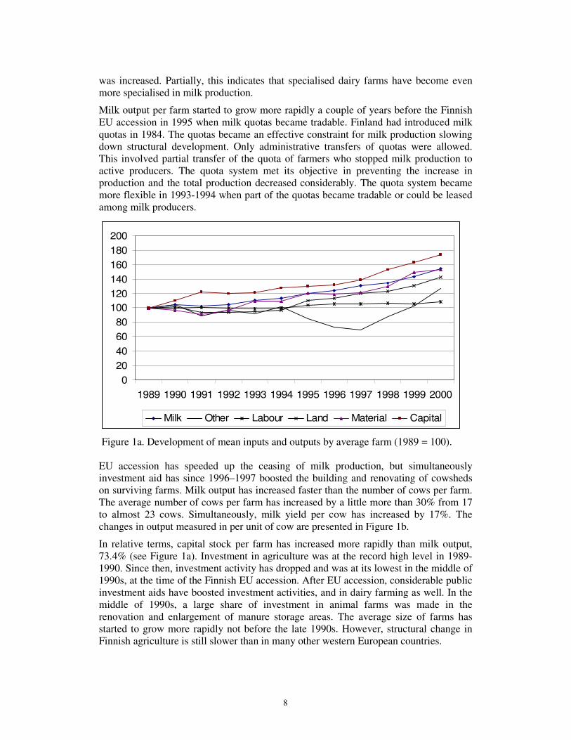
Finnish farms are typically small. Table 1 shows that the mean arable land area of the sample farms was 28.6 hectares, with the number of cows being 19. Milk output was on average 144,000 litres. In 1990, milk output per farm has increased almost by 55% but the quantity of other outputs increased only slightly (Figure 1a). In fact, it decreased after EU accession. The fall is probably partially induced by the value changes in inventories and the need to use more animals for reproduction when the number of cows

8

was increased. Partially, this indicates that specialised dairy farms have become even more specialised in milk production.

Milk output per farm started to grow more rapidly a couple of years before the Finnish EU accession in 1995 when milk quotas became tradable. Finland had introduced milk quotas in 1984. The quotas became an effective constraint for milk production slowing down structural development. Only administrative transfers of quotas were allowed. This involved partial transfer of the quota of farmers who stopped milk production to active producers. The quota system met its objective in preventing the increase in production and the total production decreased considerably. The quota system became more flexible in 1993-1994 when part of the quotas became tradable or could be leased among milk producers.

020406080

100120140160180200

1989 1990 1991 1992 1993 1994 1995 1996 1997 1998 1999 2000

Milk Other Labour Land Material Capital

Figure 1a. Development of mean inputs and outputs by average farm (1989 = 100). EU accession has speeded up the ceasing of milk production, but simultaneously investment aid has since 1996–1997 boosted the building and renovating of cowsheds on surviving farms. Milk output has increased faster than the number of cows per farm. The average number of cows per farm has increased by a little more than 30% from 17 to almost 23 cows. Simultaneously, milk yield per cow has increased by 17%. The changes in output measured in per unit of cow are presented in Figure 1b.

In relative terms, capital stock per farm has increased more rapidly than milk output, 73.4% (see Figure 1a). Investment in agriculture was at the record high level in 1989-1990. Since then, investment activity has dropped and was at its lowest in the middle of 1990s, at the time of the Finnish EU accession. After EU accession, considerable public investment aids have boosted investment activities, and in dairy farming as well. In the middle of 1990s, a large share of investment in animal farms was made in the renovation and enlargement of manure storage areas. The average size of farms has started to grow more rapidly not before the late 1990s. However, structural change in Finnish agriculture is still slower than in many other western European countries.

9

020406080

100120140160180200

1989 1990 1991 1992 1993 1994 1995 1996 1997 1998 1999 2000

Milk Other Labour Land Material Capital

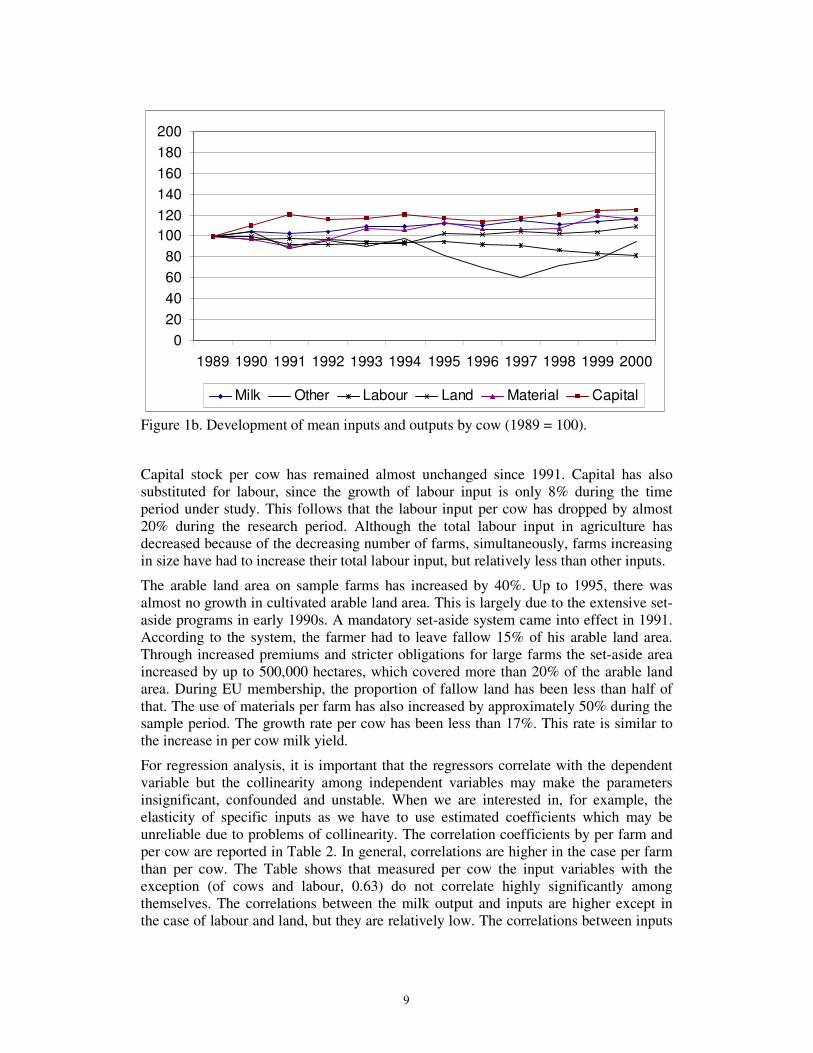
Figure 1b. Development of mean inputs and outputs by cow (1989 = 100).

Capital stock per cow has remained almost unchanged since 1991. Capital has also substituted for labour, since the growth of labour input is only 8% during the time period under study. This follows that the labour input per cow has dropped by almost 20% during the research period. Although the total labour input in agriculture has decreased because of the decreasing number of farms, simultaneously, farms increasing in size have had to increase their total labour input, but relatively less than other inputs.

The arable land area on sample farms has increased by 40%. Up to 1995, there was almost no growth in cultivated arable land area. This is largely due to the extensive set-aside programs in early 1990s. A mandatory set-aside system came into effect in 1991. According to the system, the farmer had to leave fallow 15% of his arable land area. Through increased premiums and stricter obligations for large farms the set-aside area increased by up to 500,000 hectares, which covered more than 20% of the arable land area. During EU membership, the proportion of fallow land has been less than half of that. The use of materials per farm has also increased by approximately 50% during the sample period. The growth rate per cow has been less than 17%. This rate is similar to the increase in per cow milk yield.

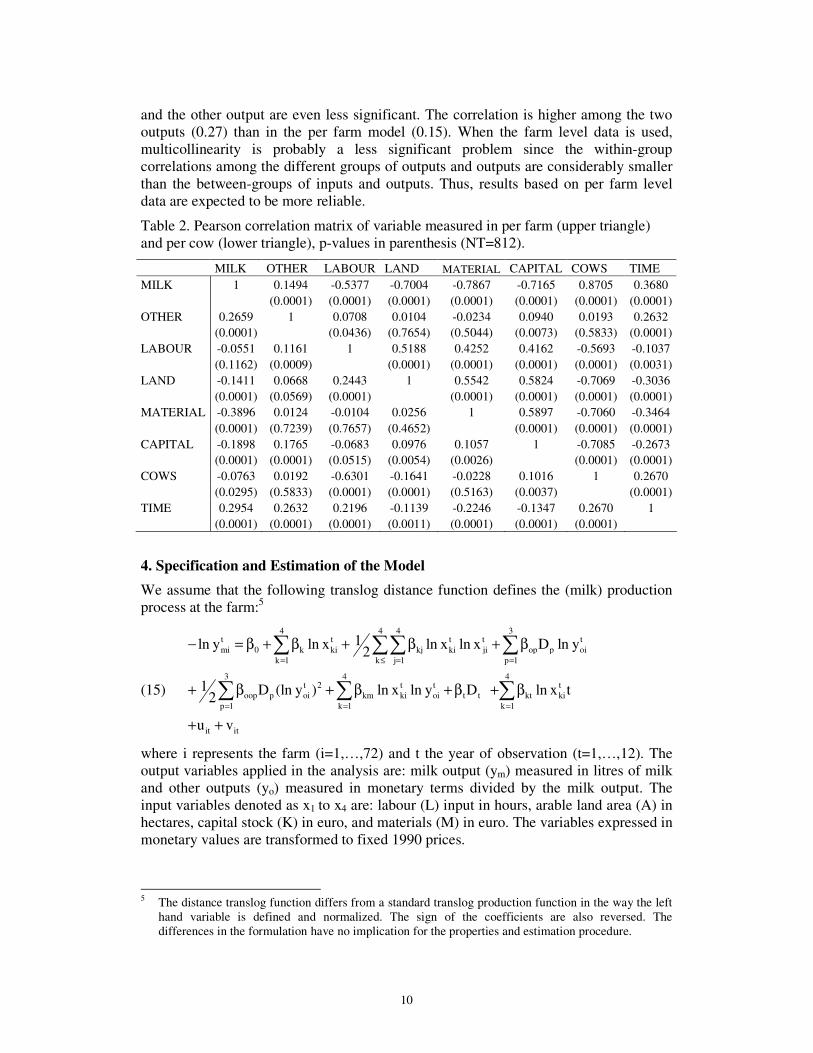
For regression analysis, it is important that the regressors correlate with the dependent variable but the collinearity among independent variables may make the parameters insignificant, confounded and unstable. When we are interested in, for example, the elasticity of specific inputs as we have to use estimated coefficients which may be unreliable due to problems of collinearity. The correlation coefficients by per farm and per cow are reported in Table 2. In general, correlations are higher in the case per farm than per cow. The Table shows that measured per cow the input variables with the exception (of cows and labour, 0.63) do not correlate highly significantly among themselves. The correlations between the milk output and inputs are higher except in the case of labour and land, but they are relatively low. The correlations between inputs

10

and the other output are even less significant. The correlation is higher among the two outputs (0.27) than in the per farm model (0.15). When the farm level data is used, multicollinearity is probably a less significant problem since the within-group correlations among the different groups of outputs and outputs are considerably smaller than the between-groups of inputs and outputs. Thus, results based on per farm level data are expected to be more reliable.

Table 2. Pearson correlation matrix of variable measured in per farm (upper triangle) and per cow (lower triangle), p-values in parenthesis (NT=812).

MILK OTHER LABOUR LAND MATERIAL CAPITAL COWS TIME MILK 1 0.1494 -0.5377 -0.7004 -0.7867 -0.7165 0.8705 0.3680

(0.0001) (0.0001) (0.0001) (0.0001) (0.0001) (0.0001) (0.0001) OTHER 0.2659 1 0.0708 0.0104 -0.0234 0.0940 0.0193 0.2632

(0.0001) (0.0436) (0.7654) (0.5044) (0.0073) (0.5833) (0.0001) LABOUR -0.0551 0.1161 1 0.5188 0.4252 0.4162 -0.5693 -0.1037

(0.1162) (0.0009) (0.0001) (0.0001) (0.0001) (0.0001) (0.0031) LAND -0.1411 0.0668 0.2443 1 0.5542 0.5824 -0.7069 -0.3036

(0.0001) (0.0569) (0.0001) (0.0001) (0.0001) (0.0001) (0.0001) MATERIAL -0.3896 0.0124 -0.0104 0.0256 1 0.5897 -0.7060 -0.3464

(0.0001) (0.7239) (0.7657) (0.4652) (0.0001) (0.0001) (0.0001) CAPITAL -0.1898 0.1765 -0.0683 0.0976 0.1057 1 -0.7085 -0.2673

(0.0001) (0.0001) (0.0515) (0.0054) (0.0026) (0.0001) (0.0001) COWS -0.0763 0.0192 -0.6301 -0.1641 -0.0228 0.1016 1 0.2670

(0.0295) (0.5833) (0.0001) (0.0001) (0.5163) (0.0037) (0.0001) TIME 0.2954 0.2632 0.2196 -0.1139 -0.2246 -0.1347 0.2670 1

(0.0001) (0.0001) (0.0001) (0.0011) (0.0001) (0.0001) (0.0001)

4. Specification and Estimation of the Model We assume that the following translog distance function defines the (milk) production process at the farm:5

(15)

4 4 4 3t t t t tmi 0 k ki kj ki ji op p oi

k 1 k j 1 p 1

3 4 4t 2 t t t

oop p oi km ki oi t t kt kip 1 k 1 k 1

it it

1ln y ln x ln x ln x D ln y2

1 D (ln y ) ln x ln y D ln x t2

u v

= ≤ = =

= = =

− = β + β + β + β

+ β + β + β + β

+ +

� �� �

� � �

where i represents the farm (i=1,…,72) and t the year of observation (t=1,…,12). The output variables applied in the analysis are: milk output (ym) measured in litres of milk and other outputs (yo) measured in monetary terms divided by the milk output. The input variables denoted as x1 to x4 are: labour (L) input in hours, arable land area (A) in hectares, capital stock (K) in euro, and materials (M) in euro. The variables expressed in monetary values are transformed to fixed 1990 prices.

5 The distance translog function differs from a standard translog production function in the way the left

hand variable is defined and normalized. The sign of the coefficients are also reversed. The differences in the formulation have no implication for the properties and estimation procedure.

11

The variables denoted as Dt are time dummies to capture year-to-year neutral technical change and Dp is the time interval for the regression coefficient of other output representing years 1989-1994, 1995-1997 and 1998-2000. The interaction of Dp and yo allows for heterogeneity in slopes associated with other outputs due to the effects of changes in policy over time and its implications for composition of outputs produced by individual farms. Non-neutral technical change is defined as a cross term of inputs or the other output and the time trend.

The error term is decomposed into two components. The first component, vit, is a standard random variable capturing effects of unexpected stochastic changes in production conditions, measurement errors in milk output or the effects of left-out explanatory variables. It is assumed to be independent and identically distributed with N(0, 2

vσ ). The second component, uit, is a non-negative random variable, associated with the technical inefficiency in production, given the level of inputs. The uits are independently distributed with a truncation at zero of N( 2,it uµ σ ), where itµ is modelled in terms of determinants of inefficiency as:

(16) 3 3

01 1

it sc sc re resc re

D Dµ δ δ δ= =

= + +� �

where Dsc refers to size class dummy variables and Dre to regional dummies. Farms were classified as small if they belonged, according to the number of cows, to the lower quartile in a specific year. Farms were classified as large ones if they belonged to the upper quartile in a specific year. Middle sized farms were those farms whose size was between lower and upper quartiles. The size classification of a farm may thus change from year to year due to structural change. In the analysis, the reference size was that of small farms. The region refers to the geographic location - Southern, Central and Northern Finland – of the farm, Central Finland being the reference group. Theδ :s are respective efficiency effects regression coefficients. The inefficiency effects part of the equation makes it possible to test whether technical efficiencies differ by size class and regional location.

The parameters of the model are estimated by the method of maximum likelihood. We applied the computer program Frontier 4.1 (Coelli 1996). The variance parameters are defined as 2 2 2

s v uσ σ σ= + and 2 2/u sγ σ σ= where γ takes the value between 0 and 1. Parameters of the stochastic frontier model can be tested using the generalised likelihood ratio statistics. Given the translog stochastic frontier specification of output distance function, technical efficiency of production can be obtained from the conditional expectation of exp( )it itTE U= − , given the random variable �it (�it.= vit - uit; Battese and Coelli 1988). The level of technical efficiency is by definition between 0 and 1, and varies across farms, and over time.

It should be noted that prior to the estimation the inputs and outputs are transformed to deviations from their sample means since each variable has been divided by its own mean. Thus, the first order coefficients are the distance elasticities at the sample mean. Linear homogeneity of outputs is imposed by dividing the two outputs by milk output. This ratio form as an explanatory variable has been discussed in the literature. Kumbhakar and Lovell (2000) have argued that the outcome of a normalisation is not independent of the choice of specific normalising output variable. Brümmer et al.

12

(2002) state, however, that the use of the norm model would lead to increasing multicollinearity and, thus, unstable estimates. Another related question is the possible endogeneity of output ratios. Coelli and Perelman (1999) have stated that transformed output variable in the ratio model are actually measures of output mix which are more likely exogenous than the variables in the norm model.6 Furthermore, according to Mundlak (1996), in the case of expected profit maximisation, the ratio variables in the production function do not suffer from endogeneity. This result can be generalised to output ratio variables in output distance functions (Brümmer et al. 2002).

5. Empirical Results

5.1 The parameter estimates Farm level estimated parameters of the output distance function described above are presented in Table 3. Several nested model specifications for the translog distance functions were estimated and tested prior to the selection of the final model. Nested likelihood ratio tests for various model specifications showed that the Cobb-Douglas specification was not a sufficient representation to describe the input-output technical relationship on Finnish dairy farms. The neutral technical change specification was also rejected against the non-neutral technical change specification (see Table 4). The hypothesis of the presence of inefficiency in the operation of farms could not be rejected either. Likelihood ratio test value for one-sided error is 111.983 indicating that the variance of inefficiency effects is a significant part of the error term variances We could also observe that the coefficients in the model explaining inefficiency were not jointly zero.

Farm level estimation results suggest that efficiency increases by size class and those farms located in the middle of Finland are technically among the most efficient farms. Thus, analyses of the result presented below are based on the specification and estimation of a stochastic frontier translog distance model incorporating both non-neutral representation of technical change and the technical efficiency effect model.

Respective estimation results per cow are presented in Appendix A. Nested likelihood specification tests showed that the full translog specification is the best specification of those considered. In the per cow case, technical efficiency increased by size class but by location, there was no significant differences.

Although the nested tests showed that the non-neutral technical change stochastic frontier translog specification is the best representation of the technology of those considered, 13 of the 39 coefficients in the regression model were not statistically significantly different from zero in the per farm model (with 18 of 39 in the per cow model).

6 In the norm model, all outputs are divided by Euclidean norm of outputs 2

iiy y= � . In the ratio

model, one of the outputs serves as denominator for all outputs.

13

Table 3. Estimated (farm level) parameters of the translog distance function, NT=812 observations.

Variable Param Coeff. Std err t-ratio Variable Param Coeff. Std err t-ratio Constant �0 0.0660 0.0232 2.8428 ln(L)2 �LL 0.1102 0.0728 1.5153 ln(Yo)89-94 �o1 0.1734 0.0205 8.4514 ln(A)2 �AA 0.1493 0.0588 2.5373 ln(Yo)95-97 �o2 0.1203 0.0166 7.2455 ln(M)2 �MM -0.1348 0.0288 -4.6879 ln(Yo)98-00 �o3 0.1340 0.0206 6.4962 ln(K)2 �KK 0.0564 0.0262 2.1548 ln(L) �L -0.2472 0.0569 -4.3454 ln(L)ln(A) �LA -0.1417 0.0976 -1.4518 ln(A) �A -0.2550 0.0501 -5.0933 ln(L)ln(M) �LM 0.0652 0.0803 0.8122 ln(M) �M -0.3035 0.0383 -7.9356 ln(L)ln(K) �LK -0.0002 0.0801 -0.0030 ln(K) �K -0.1038 0.0363 -2.8611 ln(A)ln(M) �AM 0.1979 0.0572 3.4574 D1990 �t2 -0.0406 0.0258 -1.5727 ln(A)ln(K) �AK -0.1889 0.0581 -3.2524 D1991 �t3 -0.0215 0.0270 -0.7940 ln(M)ln(K) �MK 0.0566 0.0502 1.1276 D1992 �t4 -0.0525 0.0252 -2.0872 ln(L)T �Lt -0.0158 0.0076 -2.0605 D1993 �t5 -0.0384 0.0254 -1.5113 ln(A)T �At -0.0115 0.0061 -1.8759 D1994 �t6 -0.0561 0.0254 -2.2070 ln(K)T �Kt 0.0046 0.0049 0.9513 D1995 �t7 -0.0122 0.0263 -0.4628 ln(M)T �Mt 0.0133 0.0048 2.7388 D1996 �t8 -0.0116 0.0264 -0.4378 Dsc1 �sc1 0.0705 0.0451 1.5619 D1997 �t9 -0.0282 0.0275 -1.0255 Dsc2 �sc2 0.2108 0.0224 9.4209 D1998 �t10 -0.0500 0.0274 -1.8251 Dre1 �reg1 -0.0880 0.0301 -2.9178 D1999 �t11 -0.0486 0.0274 -1.7749 Dre2 �reg2 -0.7340 0.3491 -2.1024 D2000 �t12 -0.1146 0.0276 -4.1500 σ2 0.0240 0.0025 9.6306 ln(Yo)289-94 �oo1 0.0256 0.0287 0.8893 γ 0.4165 0.0853 4.8820 ln(Yo)295-97 �oo2 0.0262 0.0069 3.7952 ln(Yo)298-00 �oo3 0.0680 0.0175 3.8912

Log likelihood test value is 519.423.

Table 3. Generalised likelihood ratio tests for parameters of the translog stochastic frontier model.

Null hypothesis Test statisticsa Critical value Cobb Douglas – no TC vs. neutral TC (d.f. 11) 50.020 19.675 Cobb Douglas – neutral TC vs. Translog – neutral TC (d.f. 13) 81.986 22.362 Translog – neutral TC vs. non-neutral TC (d.f. 4) 121.080 9.488 No technical inefficiency (d.f. 5)b 111.983 14.325 No technical efficiency effect (d.f. 4) 111.506 9.488 a Log likelihood ratio test -2(logL(H0)-logL(H1)) b The critical value is obtained from Table 1 in Kodde and Palm (1986) which shows the statistics for a

mixed Chi-square distribution with degrees of freedom equal to 5.

5.2 The distance elasticities The first order coefficients as expected show that, at the sample mean, the output distance function is decreasing in inputs and increasing in outputs. In the per farm model, the distance elasticities are highest for labour, land and materials. The per cow model is largest for materials. The elasticity of capital is always the lowest. However, input elasticities should be negative at every point.7 Otherwise the scale elasticity will

7 Due to the functional form and negative sign on the front of dependent variable, the sign of the

coefficients are reversed. Here, a negative input elasticity is interpreted as output is increasing in inputs.

14

be biased. Therefore, Table 5 shows the number of positive and negative point elasticities.

In the upper part of the Table, per farm results show that input elasticities for labour, land and materials are negative at every point of observation. For capital input, the monotonicity fails to hold in 41.5% of observations. Thus, we can conclude that the effect of scale economies cannot be measured accurately for the whole sample. The magnitude of bias should however be very small as the capital elasticity is the smallest, only -0.058 and insignificant.

In the lower part of Table 5, per cow results indicate monotonicity violations in other elasticities except materials, the elasticity of labour being the most often violated. The number of violations is approximately equal both in per farm and per cow models. In the per cow case, the magnitude of bias is probably larger since the mean elasticities of land and labour are higher and more significant than that of capital.

Table 5. Monotonicity of elasticities in the per farm and per cow model formulations.

Elasticities per farm Mean Std errora t-value Positive Negative Milk output (Ym) 0.852 812 0 Other output (Yo) 0.148 0.016 9.250 810 2 Labour (L) -0.354 0.106 -3.336 0 812 Land (A) -0.333 0.090 -3.704 0 812 Materials (M) -0.272 0.069 -3.925 0 812 Capital (K) -0.058 0.068 -0.855 337 475 Returns to scale Decreasing RTS Increasing or constant RTS Scale elasticityb -0.967 0.099 -9.748 323 152

Elasticities per cow Mean Std errora t-value Positive Negative Milk output (Ym) 0.892 Other output (Yo) 0.108 0.013 8.438 812 0 Labour (L) -0.146 0.072 -2.042 87 725 Land (A) -0.144 0.077 -1.860 163 649 Materials (M) -0.229 0.064 -3.561 0 812 Capital (K) -0.077 0.058 -1.334 110 702 Returns to scale Decreasing RTS Increasing or constant RTS Scale elasticityb -0.590 0.125 -4.724 543 6 a Standard errors calculated at the sample mean. b Includes only observations not violating monotonicity.

When standard errors of some regression coefficients are large, the standard errors8 of calculated elasticities also become large. The elasticity of capital is the only insignificant elasticity among the inputs. Another problem related to input elasticities

8 The standard errors for individual input elasticities are obtained using the delta method. It gives the distribution of a function of random variables for which one has a distribution. In our case, standard errors

for elasticities of xk are obtained from the square root of the diagonal elements of '( ) cov( , )( )

k k

y yx xy x∂ ∂

∂ ∂

(Heshmati 2001).�

15

and the decomposition of productivity changes is that the correlations between several variables are high. This multicollinearity in inputs may also affect the reliability of individual coefficients and associated input elasticities.

The average scale elasticity in the per farm model is less than 1.0 indicating on the average decreasing returns to scale (RTS). In 68% of observations, RTS is decreasing, while in 32% it is increasing. In the per cow model, RTS is increasing only in 1% of cases and the average scale elasticity is less than 0.6. Thus, a 1% growth in all inputs per cow produces a 0.6 percent increase in output. In Table 5, scale elasticity is calculated only for those observations where the monotonicity condition is not violated. An inclusion of the violating observations in the calculation will bias upward (less negative) the scale measure.

The sample mean scale elasticity based on the per farm model with the exception of 1989, 1990 and 1995 does not differ significantly from constant returns to scale in any of the observed years. Over time, the sample average RTS has increased slightly but we have to take into account that the number of valid observations decreases at the same time. In the per cow case, RTS is in every year significantly less than one but the scale elasticity is steadily increasing over time.

Table 6. Mean distance elasticities over time per farm and per cow models.

Year/Model

Milk Other output Labour Land Materials Capital RTS Per farm 1989 0.818 0.182 -0.263 -0.258 -0.311 -0.100 -0.928 1990 0.818 0.182 -0.283 -0.291 -0.297 -0.086 -0.952 1991 0.823 0.177 -0.290 -0.346 -0.292 -0.069 -0.973 1992 0.820 0.180 -0.304 -0.333 -0.298 -0.057 -0.977 1993 0.823 0.177 -0.317 -0.322 -0.304 -0.049 -0.966 1994 0.821 0.179 -0.334 -0.340 -0.294 -0.044 -0.971 1995 0.881 0.119 -0.353 -0.322 -0.278 -0.050 -0.951 1996 0.888 0.112 -0.374 -0.337 -0.263 -0.041 -0.973 1997 0.897 0.103 -0.394 -0.350 -0.249 -0.042 -0.980 1998 0.878 0.122 -0.411 -0.364 -0.239 -0.045 -1.017 1999 0.872 0.128 -0.424 -0.349 -0.242 -0.036 -0.976 2000 0.861 0.139 -0.448 -0.355 -0.221 -0.025 -0.985 Average 0.852 0.148 -0.354 -0.333 -0.272 -0.058 -0.967 Per cow 1989 0.892 0.108 -0.108 -0.142 -0.210 -0.070 -0.510 1990 0.891 0.109 -0.118 -0.144 -0.220 -0.070 -0.530 1991 0.888 0.112 -0.126 -0.138 -0.253 -0.079 -0.574 1992 0.890 0.110 -0.140 -0.147 -0.244 -0.081 -0.586 1993 0.887 0.113 -0.153 -0.151 -0.234 -0.085 -0.583 1994 0.889 0.111 -0.156 -0.134 -0.241 -0.083 -0.597 1995 0.922 0.078 -0.152 -0.122 -0.225 -0.077 -0.560 1996 0.917 0.083 -0.148 -0.139 -0.229 -0.073 -0.584 1997 0.910 0.090 -0.148 -0.150 -0.229 -0.072 -0.605 1998 0.866 0.134 -0.163 -0.156 -0.232 -0.079 -0.628 1999 0.871 0.129 -0.164 -0.147 -0.217 -0.082 -0.647 2000 0.881 0.119 -0.151 -0.156 -0.214 -0.072 -0.635 Average 0.892 0.108 -0.146 -0.144 -0.229 -0.077 -0.590

16

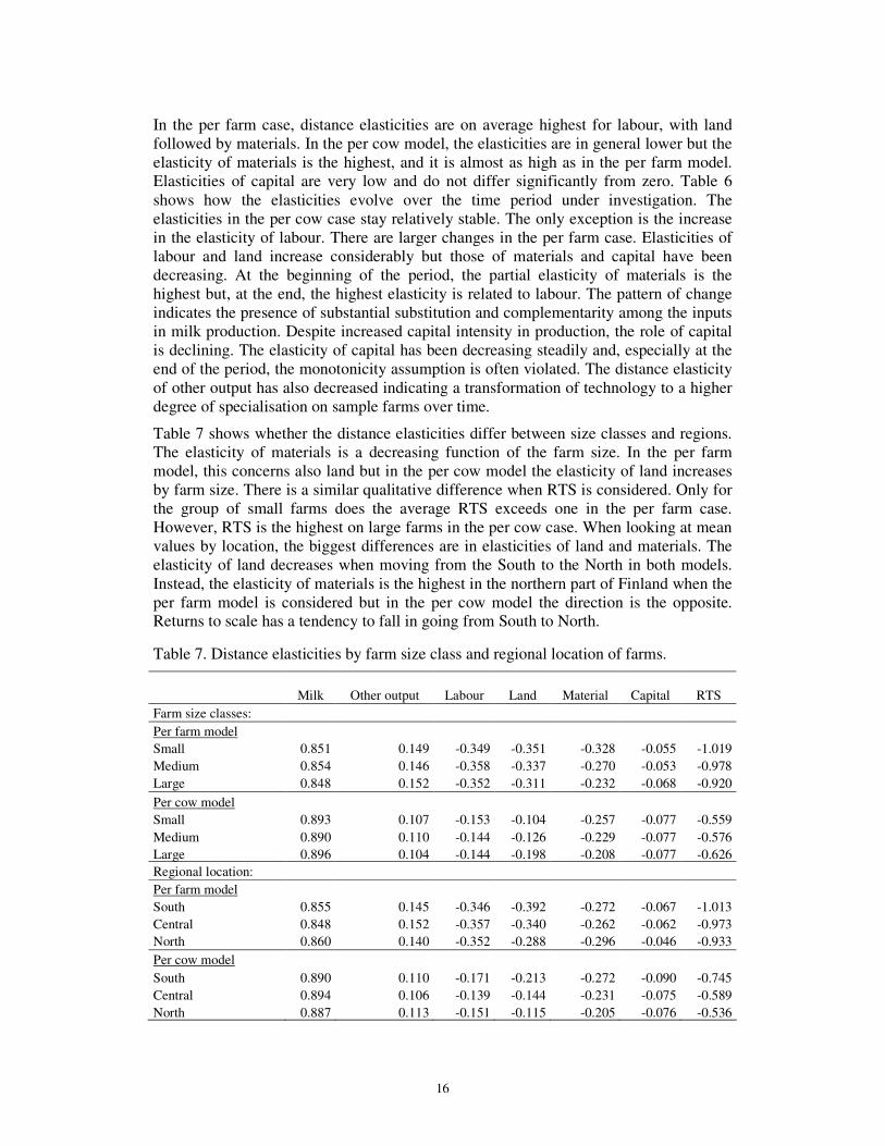
In the per farm case, distance elasticities are on average highest for labour, with land followed by materials. In the per cow model, the elasticities are in general lower but the elasticity of materials is the highest, and it is almost as high as in the per farm model. Elasticities of capital are very low and do not differ significantly from zero. Table 6 shows how the elasticities evolve over the time period under investigation. The elasticities in the per cow case stay relatively stable. The only exception is the increase in the elasticity of labour. There are larger changes in the per farm case. Elasticities of labour and land increase considerably but those of materials and capital have been decreasing. At the beginning of the period, the partial elasticity of materials is the highest but, at the end, the highest elasticity is related to labour. The pattern of change indicates the presence of substantial substitution and complementarity among the inputs in milk production. Despite increased capital intensity in production, the role of capital is declining. The elasticity of capital has been decreasing steadily and, especially at the end of the period, the monotonicity assumption is often violated. The distance elasticity of other output has also decreased indicating a transformation of technology to a higher degree of specialisation on sample farms over time.

Table 7 shows whether the distance elasticities differ between size classes and regions. The elasticity of materials is a decreasing function of the farm size. In the per farm model, this concerns also land but in the per cow model the elasticity of land increases by farm size. There is a similar qualitative difference when RTS is considered. Only for the group of small farms does the average RTS exceeds one in the per farm case. However, RTS is the highest on large farms in the per cow case. When looking at mean values by location, the biggest differences are in elasticities of land and materials. The elasticity of land decreases when moving from the South to the North in both models. Instead, the elasticity of materials is the highest in the northern part of Finland when the per farm model is considered but in the per cow model the direction is the opposite. Returns to scale has a tendency to fall in going from South to North.

Table 7. Distance elasticities by farm size class and regional location of farms.

Milk Other output Labour Land Material Capital RTS Farm size classes: Per farm model Small 0.851 0.149 -0.349 -0.351 -0.328 -0.055 -1.019 Medium 0.854 0.146 -0.358 -0.337 -0.270 -0.053 -0.978 Large 0.848 0.152 -0.352 -0.311 -0.232 -0.068 -0.920 Per cow model Small 0.893 0.107 -0.153 -0.104 -0.257 -0.077 -0.559 Medium 0.890 0.110 -0.144 -0.126 -0.229 -0.077 -0.576 Large 0.896 0.104 -0.144 -0.198 -0.208 -0.077 -0.626 Regional location: Per farm model South 0.855 0.145 -0.346 -0.392 -0.272 -0.067 -1.013 Central 0.848 0.152 -0.357 -0.340 -0.262 -0.062 -0.973 North 0.860 0.140 -0.352 -0.288 -0.296 -0.046 -0.933 Per cow model South 0.890 0.110 -0.171 -0.213 -0.272 -0.090 -0.745 Central 0.894 0.106 -0.139 -0.144 -0.231 -0.075 -0.589 North 0.887 0.113 -0.151 -0.115 -0.205 -0.076 -0.536

17

5.3 Technical efficiency In the per farm model, technical efficiency (TE) on the sample farms was on average 0.933 and the standard deviation being 0.053. This would mean that the farms should on average be able to increase their outputs by 6.7% without increasing their input use. The per cow model indicates slightly smaller efficiency: TE is 0.904 and standard deviation 0.052. The average efficiencies are relatively high compared to the efficiency scores obtained by other model specifications (e.g. Sipiläinen 2003). Sipiläinen used data envelopment analysis (DEA) to obtain efficiency scores. The DEA does not distinguish between inefficiency and random error terms. A composed effect is labelled as inefficiency which explains the lower efficiency resulted from the use of DEA based on the same data. However, in this study, the efficiency scores are not directly comparable to those of Sipiläinen since different methods and models are used. Empirical evidence suggests that the level of efficiency is not independent of the estimation or computation method. The maximum technical efficiency (TE) is 0.990 and the minimum 0.674 in the per farm case. The respective values in the per cow model are 0.980 and 0.543.

The point efficiency estimates do not have a standard error. Therefore we cannot infer about their significance levels. Confidence intervals for individual point estimates of technical efficiency scores were obtained using the approach proposed by Horrace and Schmidt (1996) and applied by Hjalmarsson et al. (1996) and Battese et al. (2000). For details on the construction of confidence intervals for the efficiency point estimates, see Appendix B.

0.75

0.8

0.85

0.9

0.95

1

1.05

1989

1990

1991

1992

1993

1994

1995

1996

1997

1998

1999

2000

Upper Efficiency Lower

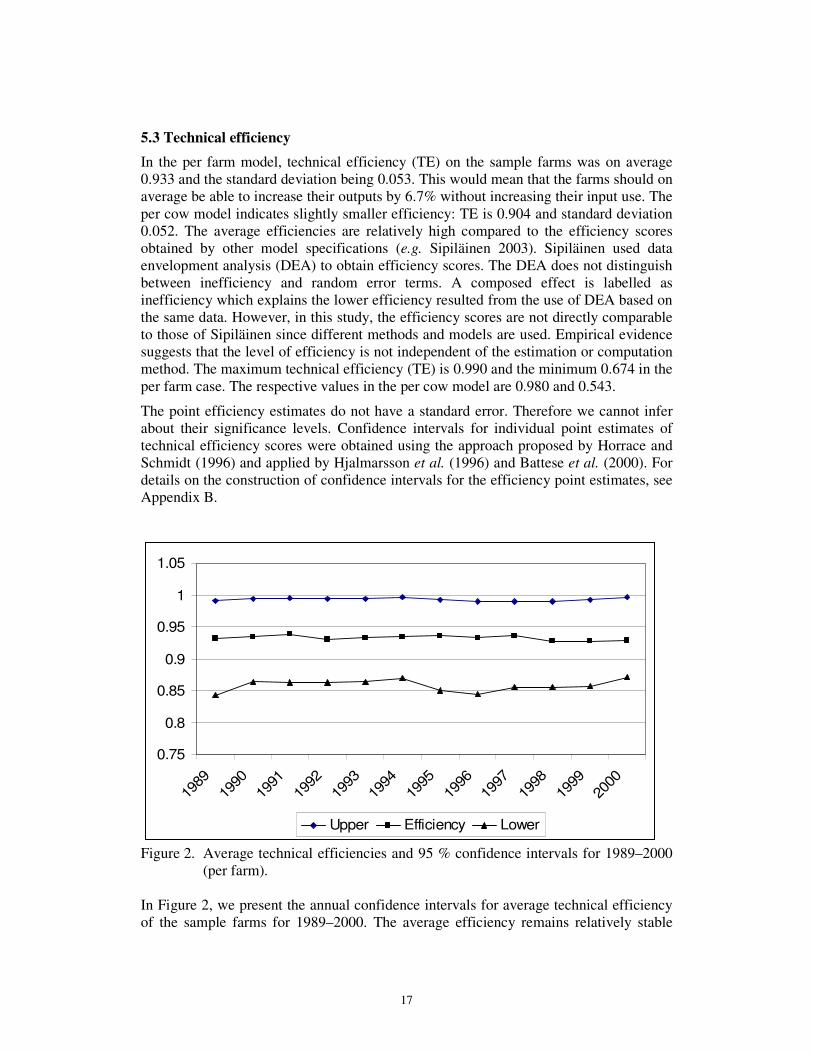
Figure 2. Average technical efficiencies and 95 % confidence intervals for 1989–2000 (per farm).

In Figure 2, we present the annual confidence intervals for average technical efficiency of the sample farms for 1989–2000. The average efficiency remains relatively stable

18

over the period. The confidence interval does not change much either. The interval is wider in 1989 and at the time of the EU accession as well as post the accession period. In 2000, the interval becomes narrower and it is as large as that found before EU accession.

Table 8 presents technical efficiencies and confidence intervals by farm size class and regional location of farms. The results suggest a positive association between efficiency and size of farms when per farm results are considered. It shows that the efficiency of small farms is on average the lowest and also the range of lower and upper limits of confidence intervals is the highest among the three groups of farms. Technical efficiency of large farms is significantly higher than that of medium sized farms, and it has a small dispersion round its mean value. It should, however, be noted that in the per cow model, we do not observe much efficiency differences between the three farm size classes. This contradicts the result of the technical efficiency effect model in the per cow model.

The average technical efficiency of farms is as expected the lowest in the northern region in both models. The width of the confidence interval is also the largest. In the per cow case, regional averages deviate less from each other than in the per farm case. It should be kept in mind as Battese et al. (2000) have stated that these confidence interval predictions may be conservative in measuring the confidence and dispersion in efficiency. Table 8. Average technical efficiencies and 95% confidence intervals by size class and regional location of farms.

Farm size classes: Lower Mean Upper Range Per farm model Small 0.786 0.883 0.981 0.195 Medium 0.841 0.925 0.994 0.153 Large 0.953 0.986 1 0.047 Per cow model Small 0.826 0.898 0.981 0.155 Medium 0.849 0.909 0.989 0.139 Large 0.853 0.898 0.988 0.135 Regional location of farm: Per farm model South 0.859 0.935 0.996 0.136 Central 0.883 0.953 0.998 0.115 North 0.799 0.882 0.980 0.181 Per cow model South 0.851 0.896 0.988 0.137 Central 0.858 0.916 0.991 0.133 North 0.811 0.878 0.977 0.165

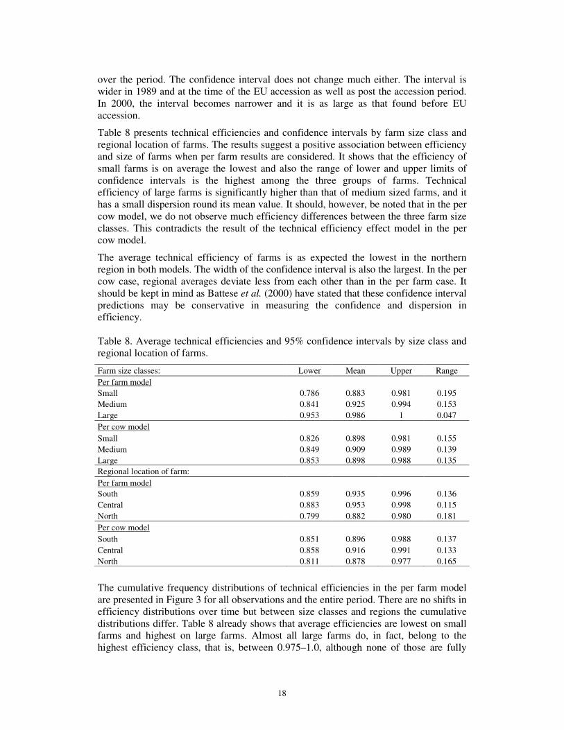
The cumulative frequency distributions of technical efficiencies in the per farm model are presented in Figure 3 for all observations and the entire period. There are no shifts in efficiency distributions over time but between size classes and regions the cumulative distributions differ. Table 8 already shows that average efficiencies are lowest on small farms and highest on large farms. Almost all large farms do, in fact, belong to the highest efficiency class, that is, between 0.975–1.0, although none of those are fully

19

efficient. On the contrary, none of the smaller farms was evaluated as highly efficient. It should be noted that the current sample consists of relatively small dairy farms and the frontier is build on the sample best practice farms, which might differ from the population best practice technology.

0

20

40

60

80

100

120

-700

7007

25

7257

50

7507

75

7758

00

8008

25

8258

50

8508

75

8759

00

9009

25

9259

50

9509

75

9759

99

All Small Medium Large

Figure 3. The cumulative distribution of technical efficiencies by size class (per farm; e.g. 700725 stands for technical efficiency of 0.700 – 0.725).

0

20

40

60

80

100

120

-700

7257

50

7507

75

7758

00

8008

25

8258

50

8508

75

8759

00

9009

25

9259

50

9509

75

9759

99

South Central North

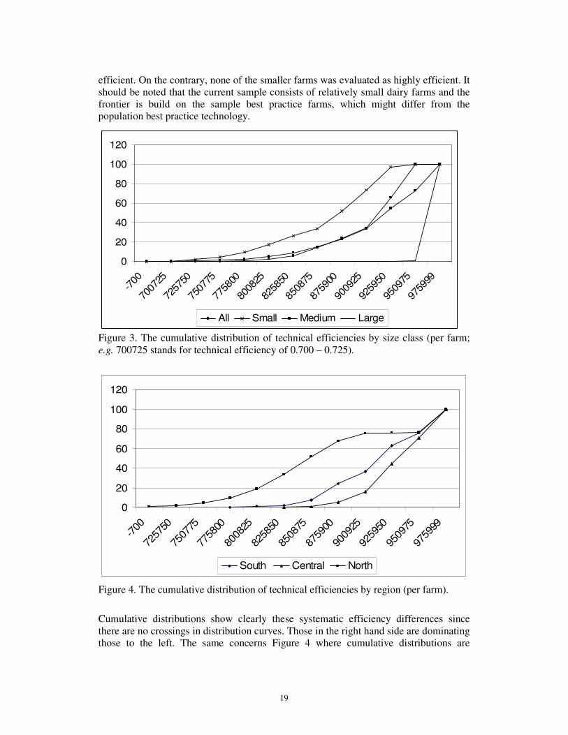
Figure 4. The cumulative distribution of technical efficiencies by region (per farm). Cumulative distributions show clearly these systematic efficiency differences since there are no crossings in distribution curves. Those in the right hand side are dominating those to the left. The same concerns Figure 4 where cumulative distributions are

20

presented by the regional location. The latter figure shows that the efficiency scores of the cumulative distribution curve are in Central Finland at every point larger than in Southern Finland. It is important to compare distributions since two series with the same mean may have different distributions.

The frequency distributions discussed above despite of being very informative cannot determine whether the dominance of one distribution over another is statistically valid or not. In the next section, we perform first and second order dominance tests by using bootstrapping techniques. The test will consider dominance in the distribution of efficiency by a number of common characteristics, such as year of observation, size of farm, regional location, capital and labour intensities.

5.4 Evaluating dominance ranking of (in)efficiency by farm attributes In this section, we examine the evolution of inefficiency, measured both at farm and at per cow levels. We employ the extended Kolmogorov-Smirnov tests of first and second order stochastic dominance as implemented by Maasoumi and Heshmati (2000). We offer partial control for many farm-specific attributes, such as size, location and production factor intensities by comparing group cells. This avoids having to specify and estimate models of dependence of inefficiency on these attributes, but lacks the multiple controls that is the promise of such techniques. We find a number of strong second order rankings between groups at the farm level but not over time or at the cow level.

5.4.1 Bootstrap procedure for dominance rankings In recent years, methods have been developed to examine the existence of uniform weak orders between welfare outcomes measured by total real incomes. Partial strong orders are commonly used in evaluation on the basis of specific utility functions and their corresponding indices of such as inequality or poverty in welfare. Such strong orderings do not command consensus. Based on the expected utility paradigm, Stochastic Dominance (SD) relations of various orders attempt to resolve this problem. In evaluating distributed outcomes, average outcomes mask the differential impact on different participants and render index based assessments as blunt instruments for policy analysis. SD analysis reveals all of the distributional changes, especially amongst the target groups. For more details on these issues see Maasoumi and Heshmati (2004) and Appendix C.

In this paper, we follow an alternative bootstrap procedure for estimating the probability of rejection of the SD hypotheses with a suitably extended Kolmogorov-Smirnov (KS) test for first and second order stochastic dominance. Alternative simulation and bootstrap implementations of this test have been examined previously by several authors including McFadden (1989), Klecan, McFadden, and McFadden (1991), Barrett and Donald (2003) and Linton et al. (2003). They prove that the resulting test is consistent against all nonparametric alternatives.

5.4.2 Testing for SD among dairy farms We compare 12 years of survey data on dairy production for the years 1989 to 2000. The data is defined in per farm and per cow levels. The efficiency in production is obtained from the estimation of a stochastic production function. For comparisons over time, we have chosen 1989, 1996 and 2000 covering both pre- and post-reform periods associated with Finland’s accession to the European Union. The years were chosen to

21

be representative as well as sufficiently far apart so that reform policy would have time to produce measurable effects. It is to be noted that for the bootstrapping test we use percent inefficiency (100-efficiency) rather than percent efficiency. This implies that the cumulative distribution function (CDF) to the right (more inefficient) are dominated by those to the left (more efficient). In addition to unconditional comparison of the inefficiency distribution over time, inefficiency is compared conditional on a number of farm characteristics used in our previous analysis. The farm characteristics that we control for are: farm size, regional location of farms, and capital and labour factor intensity in production.

In defining farm size, we have divided the sample into three groups: small, medium and large. As to regional location, the sample is divided into South, Central and North. For the factor intensity, the sample is divided by intensity in the use of capital and labour in production into three groups: low, medium and high factor intensities. Small size and low factor intensity correspond to the first quartile, the medium to the second and third quartiles, while large size and high factor density to the fourth quartile of the distribution of size and factor intensities, respectively. Our analysis is carried out in two parts. Part one comprises unconditional tests for SD over the years for the entire distribution of inefficiency, with no controls for farm attributes. Part two comprises conditional tests by having controls for the above attributes. Summary statistics of the two inefficiency definitions by farm and by cow and various sub-groups of farms are given in the first parts of Appendix C, Table C1-C5. In the second part of the above Tables, the dominance test results including the means, standard errors and probabilities are reported. Graphs of the CDF by various sub-groups and data levels are found in Appendix C, Figure C1-C5.

All results are based on 1,000 bootstrap samples, with 5% inefficiency partitions. In comparing two distributions, the first group is denoted the X-distribution, and the second by Y-distribution. Thus, FSDxoy denotes first order stochastic dominance of X over Y, and SSDxoy is similarly defined for second order dominance of X over Y. The FOmax and SOmax denote the joint tests of X vs. Y and Y vs. X., referred to as maximality by McFadden (1989). The probability (denoted as “prob” in the Tables) rejects the null of no dominance when the statistics are negative.

5.4.3 The dominance test results This first part of Table C1 summarizes our data by years of observation. The second part of the period is based on a balanced panel. The mean inefficiency does not change from 1989 (9.64) to 2000 (9.62) when inefficiency is based on cow level data. The corresponding inefficiency according to the farm level is increasing slightly from 6.85 to 7.08. The standard deviations are diminishing over time. In the second part of Table C1, our test statistics are summarized by their mean and standard errors, as well as the probability of the test statistic being negative or zero (the null hypothesis). None of the six test cases indicate presence of any first or second order dominance over time regardless of unit of observation. The distributions of inefficiency over time are not first and second order maximal (unrankable). The farm level inefficiency distributions dominate the cow levels (see Figure C1).

As mentioned previously, the farms are distinguished by the farm characteristics. Table C2 summarizes the results for different size classes, and separately for the two per farm and per cow units of measurement. The mean inefficiency and its dispersion measured

22

by per farm is a decreasing function of the farm size. No such relationship is found when the inefficiency is obtained by per cow data. The inefficiency is related to the optimality of the size of farm but not to the productivity of cows. The second part of Table C2 shows that there is no FSD or SSD between size classes when inefficiency measured by the cow level data. However, there is SSD when inefficiency is measured at the farm level where large farms SSD dominate the small and medium size farms (see also Figure C2). The distribution of inefficiency by size class is second order maximal.

Table C3 summarizes the results for different regional locations. The mean inefficiency measured at the farm level is not a clearly increasing function of the distance from the fertile South. The sub-sample of South is quite small. Farms located in Central Finland are better off in terms of inefficiency and its dispersion regardless of the level of measurement. When measured at the cow level, North weakly SSD dominates the Central location. However, when measured at the farm level North SSD dominates both Central and South regions (see Figure C3). The distributions of inefficiency by location measured at the farm level are second order maximal.

Comparisons of distribution by capital intensity are reported in Table C4. Unlike in the case of farm size, the inefficiency and its variation is increasing by degree of capital intensity when results are based on the cow level data. A low level of capital intensity is the most optimal when distribution is analyzed at the cow level. No such distinction is made at the farm level. The low and high intensity levels are second order maximal in both definition cases (see also Figure C4).

Table C5 provides a summary of the results for different labour intensities in production. At both units of measurement, inefficiency in production is positively associated with labour intensity. However, at the cow level no first or second order dominance is observed. The distributions at this level are not rankable. On the other hand, at the farm level higher labour intensity SSD dominates the lower levels of labour intensity (Figure C5). The distributions here are second order maximal. It is worth recalling that SD rankings are transitive.

In summary, the test results based on the sample of dairy farms over time are basically the same regardless of the farm or cow unit of observation. The average inefficiency and its dispersion are found to be quite constant over time. Based on our implementation of the KS type FSD and SSD tests, we were able to show a number of cases of dominance between conditional inefficiency distributions. These rankings are due to many other characteristics that may explain inefficiency differentials between subgroups of farms. Here the examination is offered by conducting SD tests for inefficiency of different groups identified by farm characteristics. Second order dominance is observed when the data is measured in per farm level but none when inefficiency is measured at the per cow level. The cows perform quite homogenously at the farm level. The differences in performance seem to a high degree be related non-cow production factors or characteristics. The farms are rankable in performance by size, location and labour intensity, but not with respect to capital intensity in production. An alternative approach to the one presented above is to examine regression-based simultaneous controls for the multiple of characteristics. In a regression-based approach, as that in Maasoumi and Heshmati (2004), one avoids the problem of small cell sizes that would arise in current approach.

23

5.5 The Components of TFP growth The productivity growth on the dairy farms in the sample is calculated applying the approach of Orea (2002). The productivity growth is decomposed to technical change, technical efficiency change and scale effect. The actual values are calculated on the basis of estimated per farm model coefficients in the translog model presented in Table 2. The TFP growth results are presented in Table 9. Table 9. Average productivity change and its components (the decomposition of Orea,

2002).

Period (per farm) Productivity Technical efficiency Neutral technical

Non-neutral technical Scale

% Change % Change % Change % Change % Effecta 1989/1990 2.92 0.38 4.06 -0.03 -1.49 1990/1991 -2.02 0.68 -1.92 -0.02 -0.76 1991/1992 2.83 -0.40 3.11 0.04 0.08 1992/1993 -1.76 -0.02 -1.41 0.05 -0.38 1993/1994 2.13 0.17 1.77 0.07 0.12 1994/1995 -3.85 0.11 -4.39 0.03 0.40 1995/1996 -0.50 -0.33 -0.06 -0.05 -0.06 1996/1997 1.87 0.29 1.67 -0.05 -0.04 1997/1998 1.22 -0.87 2.18 0.01 -0.10 1998/1999 0.05 -0.02 -0.15 0.10 0.12 1999/2000 6.83 0.21 6.61 0.12 -0.11 Per farm values: Cumulative 9.72 0.20 11.47 0.27 -2.23 Annual average 0.88 0.02 1.04 0.02 -0.20 Per cow unit values: Cumulative 8.60 0.19 9.38 0.05 -1.02 Annual average 0.78 0.02 0.85 0.00 -0.09

a Calculated as a distance from 1 only for those observations, which do not violate monotonicity restriction.

According to the analysis, productivity growth on dairy farms has been low during the 1990s. The patterns are similar both in per farm and in per cow models. The average productivity growth is 0.9% (0.8% at the cow level) interpreted as the annual growth rate in output larger than the weighted average growth in inputs. High growth rates were observed both at the beginning and at the end of the decade. Before EU accession in 1995, productivity growth varied from positive to negative in sequential years. Slow productivity growth is probably a result of several production restrictions, which were in use or were introduced during that period. At the time of EU accession in 1995, the productivity declined significantly. This drop may partially be caused by data when the prices changed drastically, principally over a single night. After EU accession in 1995, productivity growth has been mostly positive. However, the growth rate has been relatively modest until the end of the research period. The annual cow level results are presented in Appendix D, Table D1.

The technical progress has mainly been based on pure (neutral) technical change. The most important sources for the progress are probably the relief of milk quota restrictions

24

and set-aside requirements. Both enlargements of the farms together with the adoption of modern production technology and good weather conditions at the end of the decade have contributed to productivity growth by shifting the production frontier upwards.

Technical efficiency change did not show any particular pattern and the changes between sequential years are found to be relatively small, as it was observed earlier. During the research period, there is practically no change in average technical efficiency as the previous chapter has already shown. The scale effect was almost negligible but its cumulative effect was negative over the research period. Even at the end of the period when milk production at the farm level increases most rapidly, the average scale effect is negative. We should also mention that the magnitude of the scale effect varies by farms. Monotonicity condition fails to hold in a large number of data points which is associated with the capital input variable in per farm case (the monotonicity in land and labour are also violated in the per cow model). The violated points are not considered in the calculation of returns to scale. Therefore, the number of observations when calculating scale effect is considerably smaller than the total number of observations in the sample.

Allocative inefficiency component is a result of the violations against the first-order condition of profit maximisation, for example, output elasticity shares of inputs deviate from their actual expenditure shares. Although the Malmquist index does not require any behavioural assumption to be made, we find it important to take into account the allocative effects. These violations may occur due to market imperfections like transactions costs, risk, quantitative restrictions, or imperfect information (Brümmer et al. 2002). Kumbhakar and Lovell (2000, p. 284) have stated that price data are required for calculating allocative inefficiencies. Aggregated cost and return data are actually sufficient for the analysis if uniform prices facing all farmers can be assumed.

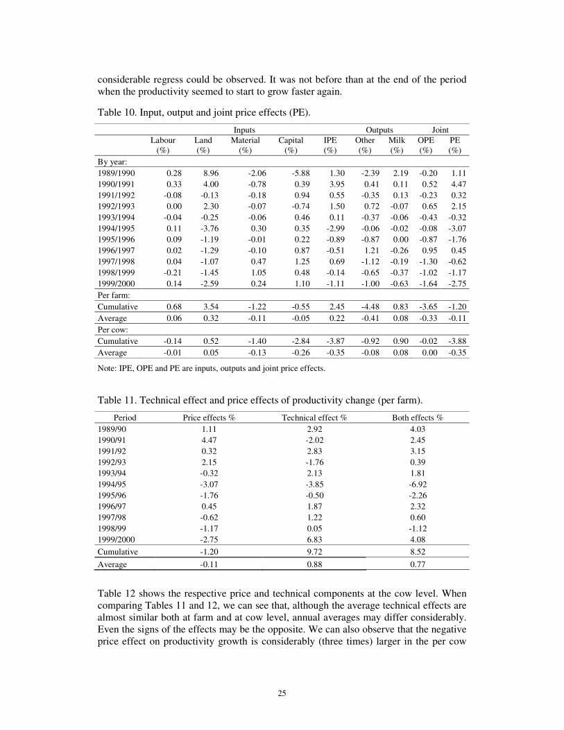
Table 10 shows the input, output and their joint price effects. When evaluated over the whole period, the price effect is negligible but on average negative. At cow level, the average effect is larger than at farm level. However, in specific years the price effects (price distortions) can be considerably larger than technical change effect. The inputs distortions are found to be largest at the beginning of the research period and at the time of the EU accession. The main source of distortions has been the land input in the farm level model but capital and material inputs in the cow level model (see Appendix D, Table D2). In the first part of the research period, compulsory set-aside programs are a probable cause of land input price distortion at the farm level model. We should also keep in mind that the rental prices of land do not necessary follow directly the productivity changes of land in the short run i.e. year-to-year variations in yield since the contracts have usually been made on a long-term basis covering several years and on the basis of fixed prices. The terms of such contracts in addition to productivity of land may also somehow reflect the expected output prices.

Over and under utilisation of resources typically varies a great deal over time and take out each other thereby the cumulative effect turns out to be relatively small. On the output side, the distortions are smaller than on the input side.

Table 11 presents the farm level joint productivity change, which consists of the sum of technical effects and price effects. Depending on the point of time these effects may accumulate or partially replace each other. The series shows that at the beginning of 1990s the productivity growth was relatively rapid but at the time of EU accession a

25

considerable regress could be observed. It was not before than at the end of the period when the productivity seemed to start to grow faster again.

Table 10. Input, output and joint price effects (PE).

Inputs Outputs Joint

Labour

(%) Land (%)

Material (%)

Capital (%)

IPE (%)

Other (%)

Milk (%)

OPE (%)

PE (%)

By year: 1989/1990 0.28 8.96 -2.06 -5.88 1.30 -2.39 2.19 -0.20 1.11 1990/1991 0.33 4.00 -0.78 0.39 3.95 0.41 0.11 0.52 4.47 1991/1992 -0.08 -0.13 -0.18 0.94 0.55 -0.35 0.13 -0.23 0.32 1992/1993 0.00 2.30 -0.07 -0.74 1.50 0.72 -0.07 0.65 2.15 1993/1994 -0.04 -0.25 -0.06 0.46 0.11 -0.37 -0.06 -0.43 -0.32 1994/1995 0.11 -3.76 0.30 0.35 -2.99 -0.06 -0.02 -0.08 -3.07 1995/1996 0.09 -1.19 -0.01 0.22 -0.89 -0.87 0.00 -0.87 -1.76 1996/1997 0.02 -1.29 -0.10 0.87 -0.51 1.21 -0.26 0.95 0.45 1997/1998 0.04 -1.07 0.47 1.25 0.69 -1.12 -0.19 -1.30 -0.62 1998/1999 -0.21 -1.45 1.05 0.48 -0.14 -0.65 -0.37 -1.02 -1.17 1999/2000 0.14 -2.59 0.24 1.10 -1.11 -1.00 -0.63 -1.64 -2.75 Per farm: Cumulative 0.68 3.54 -1.22 -0.55 2.45 -4.48 0.83 -3.65 -1.20 Average 0.06 0.32 -0.11 -0.05 0.22 -0.41 0.08 -0.33 -0.11 Per cow: Cumulative -0.14 0.52 -1.40 -2.84 -3.87 -0.92 0.90 -0.02 -3.88 Average -0.01 0.05 -0.13 -0.26 -0.35 -0.08 0.08 0.00 -0.35

Note: IPE, OPE and PE are inputs, outputs and joint price effects.

Table 11. Technical effect and price effects of productivity change (per farm).

Period Price effects % Technical effect % Both effects % 1989/90 1.11 2.92 4.03 1990/91 4.47 -2.02 2.45 1991/92 0.32 2.83 3.15 1992/93 2.15 -1.76 0.39 1993/94 -0.32 2.13 1.81 1994/95 -3.07 -3.85 -6.92 1995/96 -1.76 -0.50 -2.26 1996/97 0.45 1.87 2.32 1997/98 -0.62 1.22 0.60 1998/99 -1.17 0.05 -1.12 1999/2000 -2.75 6.83 4.08 Cumulative -1.20 9.72 8.52 Average -0.11 0.88 0.77

Table 12 shows the respective price and technical components at the cow level. When comparing Tables 11 and 12, we can see that, although the average technical effects are almost similar both at farm and at cow level, annual averages may differ considerably. Even the signs of the effects may be the opposite. We can also observe that the negative price effect on productivity growth is considerably (three times) larger in the per cow

26

model than in the per farm model. This follows that the average annual productivity growth over the whole period is only 0.43% at the cow level when at the farm level a growth rate of 0.77% is shown. This indicates that the growth of farms in respect to the number of animals is an important source of productivity growth.

Table 12. Technical effect and price effects of productivity change (per cow).

Period Price effect. % Technical effect. % Both effects. % 1989/90 -1.73 1.61 -0.12 1990/91 5.31 -7.28 -1.97 1991/92 -1.83 3.90 2.08 1992/93 1.15 3.05 4.21 1993/94 -0.40 0.80 0.40 1994/95 -3.01 0.92 -2.09 1995/96 0.33 -3.49 -3.17 1996/97 -0.36 3.32 2.97 1997/98 0.05 -1.32 -1.26 1998/99 -0.38 1.70 1.33 1999/2000 -3.02 5.37 2.35 Cumulative -3.88 8.60 4.72 Average -0.35 0.78 0.43

6. Discussion of the Results and Conclusions

In this paper, we have studied the productivity change applying the Malmquist productivity index. Several suggestions have been made to decompose the index in order to define the sources of productivity growth (e.g. Färe et al. 1994, Ray and Desli 1997, Lovell 2003). Many of the applications have been nonparametric. In our case, we have identified the components of productivity growth from the stochastic output distance function. We have applied the approaches suggested by Orea (2002), Brümmer et al. (2002) and Kumbhakar and Lovell (2000).

In Orea’s (2002) decomposition of the Malmquist index, the specification of scale effect does not lean on the concept of scale efficiency and scale efficiency change as often is the case in nonparametric approach. It is possible to calculate also for Cobb-Douglas and ray-homogenous technologies. In our case, neither of the previously mentioned technologies are adequate representations of the production technology in Finnish dairy farming.

Productivity growth was relatively slow in the 1990s but it speeded up at the end of the study period. The growth related mostly to technical change. The result is reasonable when taking into account that the enlargement investments on dairy farms started to increase in 1996-1997 because of the introduction of state-sponsored investment subsidies and less restrictive policies. Simultaneously milk quota restrictions and set-aside requirements were relieved. Uncertainties related to EU accession in 1995 were also likely to postpone farmers’ development strategies and their implementations.

Technical efficiency change does not show any systematic pattern over the research period. Technical efficiency varied over time, which was partially linked to weather conditions. The Finnish production system is largely based on on-farm produced feed. The quantity and quality of this feed depends on the weather, thus affecting the need to purchase externally produced inputs. The weather has also a direct effect on milk

27

production. Since the weather conditions may differ in different regions of the country within a year, it may influence the variation in the technical efficiency. The stochastic weather conditions may also affect the general shift of the frontier, i.e. technical change effect.

According to the analysis, EU accession did not seem to have a significant effect on technical efficiency. Instead, farm size and regional location could explain a significant share of the variation in technical efficiency among dairy farms at the farm level analysis. The test results for stochastic dominance over time are basically the same regardless of the unit of observation, per farm or per cow. However, we were able to show a number of cases of dominance between conditional inefficiency distributions. These rankings are due to many characteristics that may explain inefficiency differentials between sub-groups of farms. Second order dominance was observed when the data were measured in per farm level but none when using per cow level data. The farms are rankable in performance by size, location and labour intensity, but not with respect to capital intensity in production.

The average returns to scale at farm level models was smaller than one but not significantly, indicating on average decreasing returns to scale. Although RTS improved during the research period, the analysis showed that the role of the scale effect in productivity growth was small. The cumulative scale effect over the whole period was slightly negative. Thus, the input output relations did not improve despite the increase in the scale of production. The distance elasticity of capital was also very low. Even the monotonicity condition (an increase in inputs also increases output) was violated at several data points at the end of the research period in the farm level model. At the cow level analysis, violations were more evenly distributed over labour, capital and land inputs.

An important issue is that why the scale effect is so small? There might be several factors resulting in the absence of positive scale effects in Finnish agriculture. One is that capital has substituted for labour. It is evident that productivity of labour increases with the capital intensity. However, family labour is often a binding restriction to the scale of operation of farms. Increased capital input has made it possible to increase production with only a relatively small increase in labour input. We can conclude that the average size of dairy farms is such that an increase in farm size, combined with appropriate capital investments, may contribute markedly on labour productivity.

There seems also to be considerable substitution effect between land and materials inputs at the farm level. The elasticity of land has increased simultaneously with the decrease in the elasticity of materials. Over time land input has increased less than milk output, but the use of materials (e.g. purchased feed) has increased by the same proportion as milk output. Despite of the input substitution, in the cow level data elasticities of land, material and capital inputs have not diminished.

The farm level distance elasticities differ considerably from those presented by Brümmer et al. (2002) and Newman and Matthews (2003). In the above mentioned studies, the largest elasticities are related to intermediate inputs (materials) but, in Finland, the elasticities of land and labour are the highest followed by materials. In all other countries, the elasticity of labour is low compared to that of Finland. The differences are probably associated with differences in farming and dairy production systems in different countries. For example, in the Netherlands, elasticity of land was

28

almost as high as in Finland and the Polish elasticity of capital is approximately as low as that of Finland (Brümmer et al. 2002). In Finland, the share of purchased feed compared to on-farm produced feed has increased over time simultaneously with the increase in milk output per farm and per cow.

The results of our analysis on productivity change are similar to those based on the DEA analysis (Sipiläinen 2003). The nonparametric analysis also indicated that the main source of productivity change was a technical change. The only major difference was in the level of technical efficiency, which was considerably lower in the DEA based analysis. However, the effect of technical efficiency change on productivity change was minor. Thus, in both approaches, the level of technical efficiency was unchanged over time.

The allocative distortions were studied by comparing actual cost and return shares to those derived on the basis of elasticities. These differences can be interpreted as deviations from the first order conditions of profit maximisation. The largest distortions were observed in land input at the farm level model but in capital and materials at the cow level model. In general, output price distortions (the deviations from the optimum) were smaller than input distortions. Over and under utilisation of resources varied considerably over time and the cumulative effects were small. However, in specific years, the average price effect may be even larger than the technical effect. The highest distortions could be observed at the beginning and at the end of the research period. In addition, the Finnish EU accession caused a considerable peak in distortions. It should be kept in mind, however, that due to milk quota restrictions, an imposition of cost minimisation behaviour could be more applicable approach than profit maximisation.

Although at the time of EU accession the prices and relative prices changed dramatically and a large share of income started to come from direct payments, technical efficiency has remained unchanged on dairy farms. The process of the EU accession seems to have affected the productivity growth, at first, as reducing and postponing investment and then as boosting it. The changes in behaviour are related both to uncertainty and support measures like investment aids. Increased investment has led to growing herd sizes in the latter part of the 1990s. The growth of farms makes it possible to utilise modern technology and improve productivity but it is too early to say if the productivity growth will speed up from the low level of less than 1% per year. Productivity growth should be faster if Finnish dairy farms wanted to keep up with, or even catch up with, dairy farms in other countries.

The study provides a detailed decomposition of productivity change taking into account both technical and price effects. The applied distance function approach is a flexible method for analysis of factors causing productivity change. Identification and separation of such effects remain unobserved when TFP index numbers are applied. This approach can also be used when the variation in prices is insufficient for cost or profit function analysis of production.

29

References Balk, B.M. 2001. Scale efficiency and productivity change. Journal of Productivity

Analysis 15:159-183. Barrett, G. & S. Donald (2003), Consistent tests for stochastic dominance,

Econometrica 71(1), 71-104. Battese, G.E. & Coelli, T.J. 1992. Frontier production functions, technical efficiency

and panel data: with applications to paddy farmers in India. Journal of Productivity Analysis 3:153-169.

Battese, G.E. & Coelli, T.J. 1988. Prediction of firm-level technical efficiencies with a generalized production function and panel data. Journal of Econometrics 38:387-389.

Battese, G.E. and Coelli, T.J. 1995. A model of technical inefficiency effects in a stochastic frontier production function for panel data. Empirical Economics 20:325-332.

Battese, G.E., Heshmati, A. & Hjalmarsson, L. 2000. Efficiency of labour use in Swedish banking industry: a stochastic frontier approach. Empirical Economics 25:623-640.

Brümmer. B., Glauben, T. & Thijssen, G. 2002. Decomposition of productivity growth using distance functions: The case of dairy farms in three European countries. American Journal of Agricultural Economics 84(3):628-644.

Caves, D.W., Christensen, L.R. & Diewert, W.E. 1982. The economic theory of index numbers and the measurement of input, output and productivity. Econometrica 50:1393-1414.

Coelli, T.J. 1996. A guide to Frontier 4.1: A computer program for stochastic frontier and cost function estimation. Centre for Efficiency and Productivity Analysis. Working Paper 96/07.

Coelli, T.J. & Perelman, S. 1999. A comparison of parametric and nonparametric distance functions: with application to European railways. European Journal of Operational Research 117:326-339.

Fuentes, H.J., Grifell-Tatjé, E. & Perelman, S. 2001. A parametric distance function approach for Malmquist productivity index estimation. Journal of Productivity Analysis 15:79-94.

Denny, M., Fuss, M. & Waverman, L. 1981. The measurement and interpretation of total factor productivity in regulated industries with an application to Canadian telecommunications. In T.G. Cowing and R.E. Stevenson (eds.) Productivity measurement in regulated industries. New York. Academic Press. p. 179-218.

Diewert, W.E. 1992. Fisher ideal output, input and productivity indexes revisited. Journal of Productivity Analysis 3/3:211-248.

Diewert, W.E. 1986. Exact and superlative index numbers. Journal of Econometrics 4:115-145.

Diewert, W.E. & Nakamura, A.O. 2003. Index number concepts, measures and decompositions of productivity growth. Journal of Productivity Analysis. 19:127-159.

Färe, R., Grosskopf, S. & Lovell, C.A.K. 1994. Production frontiers. Cambridge

30

University Press. Cambridge. Färe, R., Grosskopf, S., Norris, M. & Zhang, Z. 1994. Productivity growth, technical

progress and efficiency change in industrialized countries. American Economic Review 84(1):66-83.

Färe, R., Grosskopf, S., Lindgren, B. & Roos, P. 1989, 1994. Productivity development in Swedish hospitals: A Malmquist output index approach. In A. Charnes, W.W. Cooper, A. Lewin and L. Seiford (eds.) Data Envelopment Analysis: theory, methodology and applications. Kluwer Academic Publishers. Boston.

Hemilä, K. 1982. Measuring technological change in agriculture: An application based on the CES production function. Journal of the Scientific Agricultural Society of Finland 54:165-223.

Heshmati, A. 2001. On the growth of micro and small firms: Evidence from Sweden. Small Business Economics 17:213-228.

Horrace, W.C. & Schmidt, P. 1996. Confidence statements for efficiency estimates from stochastic frontier models. Journal of Productivity Analysis 7:257-282.

Ihamuotila, R. 1972. Productivity and the aggregate production function in the Finnish agricultural sector, 1950-1969. Working paper of Agricultural Economics Research Institute of Finland. No. 25.

Klecan, L., R. McFadden, & D. McFadden (1991), A robust test for stochastic dominance, Working Paper, Department of Economics, MIT.

Kodde, D.A. & F.C., Palm. 1986. Wald Criteria for jointly testing equality and inequality restrictions. Econometrica 54(5), 1234-1248.

Kumbhakar, S.C. & Lovell, C.A.K. 2000. Stochastic frontier analysis. Cambridge University Press.

Linton, O., E. Maasoumi & Y-J. Whang (2003), Consistent testing for stochastic dominance under general sampling schemes, Cowles Foundation, SMU, and the LSE EM/02/433.

Lovell, C.A.K. 2003. The decomposition of Malmquist productivity indexes. Journal of Productivity Analysis 20:437-458.

Maasoumi, E. & A. Heshmati (2000), Stochastic dominance amongst Swedish income distributions, Econometric Reviews 19(3), 287-320.

Maasoumi, E. & A. Heshmati (2004), Evaluating dominance ranking of PSID incomes by various household attributes, Unpublished Manuscript.

Malmquist, S. 1953. Index numbers and indifference surfaces. Trabajos de Estatística 4:209-242.

McFadden, D. (1989), Testing for stochastic dominance, in Part II of T. Fomby and T.K. Seo (eds.) Studies in the economics of uncertainty (in honour of J. Hadar), Springer-Verlag.

Mundlak, Y. 1996. Production function estimation: Reviving the primal. Econometrica 64(March):431-438.

Myyrä, S. & Pietola, K. 1999. Tuottavuuskehitys Suomen maataloudessa 1987-97. Maatalouden taloudellinen tutkimuslaitos (MTTL). Tutkimuksia 234. 57 p.

Nadiri, I.M. 1970. Some approaches to the theory and measurement of total factor productivity: A survey. Journal of Economic Literature 8:1137-1177.

31

Newman, C. & Matthews, A. 2003. The productivity performance of Irish dairy farms 1984-2000: a multiple output distance function approach. Paper presented in the Eighth European Workshop on Efficiency and Productivity Analysis. Oviedo. Spain. September 2003. 25 p.

Nishimizu, M. & Page, J.M. 1981. Total factor productivity growth, technological change and technical efficiency change. Economic Journal. 92(December 1981): 920-936.

Orea, L. 2002. Parametric decomposition of a generalized Malmquist productivity index. Journal of Productivity Analysis 18:5-22.

Ray, S.C. 1998. Measuring scale efficiency from a translog production function. Journal of Productivity Analysis 11:183-194.

Ray, S.C. & Desli, E. 1997. Productivity growth, technical progress and efficiency change in industrialized countries: Comment. American Economic Review 87(5):1033-1039.

Ryhänen, M. 1994. Input substitution and technological development on Finnish dairy farms for 1965-1991. Agricultural Science in Finland 3:525:599.

Sims, E. 1994. The rate of technical change in Finnish agriculture, 1960-1990. Agricultural Science in Finland 3:151-160.

Sipiläinen, T. 2003. Suurten maito- ja viljatilojen suorituskyky ja sen kehittäminen. Helsingin yliopisto. Taloustieteen laitos. Julkaisuja 38. 90 p.

Ylätalo, M. 1987. Maatalouden tuottavuus ja investoinnit. Pellervon taloudellisen tutkimuslaitoksen julkaisuja No. 8.

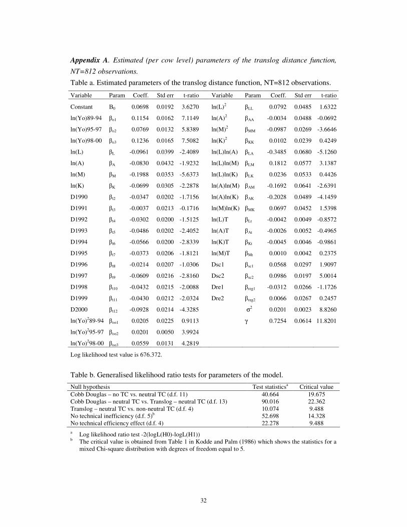
32

Appendix A. Estimated (per cow level) parameters of the translog distance function,

NT=812 observations.

Table a. Estimated parameters of the translog distance function, NT=812 observations.

Variable Param Coeff. Std err t-ratio Variable Param Coeff. Std err t-ratio

Constant �0 0.0698 0.0192 3.6270 ln(L)2 �LL 0.0792 0.0485 1.6322

ln(Yo)89-94 �o1 0.1154 0.0162 7.1149 ln(A)2 �AA -0.0034 0.0488 -0.0692

ln(Yo)95-97 �o2 0.0769 0.0132 5.8389 ln(M)2 �MM -0.0987 0.0269 -3.6646

ln(Yo)98-00 �o3 0.1236 0.0165 7.5082 ln(K)2 �KK 0.0102 0.0239 0.4249

ln(L) �L -0.0961 0.0399 -2.4089 ln(L)ln(A) �LA -0.3485 0.0680 -5.1260

ln(A) �A -0.0830 0.0432 -1.9232 ln(L)ln(M) �LM 0.1812 0.0577 3.1387

ln(M) �M -0.1988 0.0353 -5.6373 ln(L)ln(K) �LK 0.0236 0.0533 0.4426

ln(K) �K -0.0699 0.0305 -2.2878 ln(A)ln(M) �AM -0.1692 0.0641 -2.6391

D1990 �t2 -0.0347 0.0202 -1.7156 ln(A)ln(K) �AK -0.2028 0.0489 -4.1459

D1991 �t3 -0.0037 0.0213 -0.1716 ln(M)ln(K) �MK 0.0697 0.0452 1.5398

D1992 �t4 -0.0302 0.0200 -1.5125 ln(L)T �Lt -0.0042 0.0049 -0.8572

D1993 �t5 -0.0486 0.0202 -2.4052 ln(A)T �At -0.0026 0.0052 -0.4965

D1994 �t6 -0.0566 0.0200 -2.8339 ln(K)T �Kt -0.0045 0.0046 -0.9861

D1995 �t7 -0.0373 0.0206 -1.8121 ln(M)T �Mt 0.0010 0.0042 0.2375

D1996 �t8 -0.0214 0.0207 -1.0306 Dsc1 �sc1 0.0568 0.0297 1.9097

D1997 �t9 -0.0609 0.0216 -2.8160 Dsc2 �sc2 0.0986 0.0197 5.0014

D1998 �t10 -0.0432 0.0215 -2.0088 Dre1 �reg1 -0.0312 0.0266 -1.1726

D1999 �t11 -0.0430 0.0212 -2.0324 Dre2 �reg2 0.0066 0.0267 0.2457

D2000 �t12 -0.0928 0.0214 -4.3285 σ2 0.0201 0.0023 8.8260

ln(Yo)289-94 �oo1 0.0205 0.0225 0.9113 γ 0.7254 0.0614 11.8201

ln(Yo)295-97 �oo2 0.0201 0.0050 3.9924

ln(Yo)298-00 �oo3 0.0559 0.0131 4.2819

Log likelihood test value is 676.372.

Table b. Generalised likelihood ratio tests for parameters of the model.

Null hypothesis Test statisticsa Critical value Cobb Douglas – no TC vs. neutral TC (d.f. 11) 40.664 19.675 Cobb Douglas – neutral TC vs. Translog – neutral TC (d.f. 13) 90.016 22.362 Translog – neutral TC vs. non-neutral TC (d.f. 4) 10.074 9.488 No technical inefficiency (d.f. 5)b 52.698 14.328 No technical efficiency effect (d.f. 4) 22.278 9.488 a Log likelihood ratio test -2(logL(H0)-logL(H1)) b The critical value is obtained from Table 1 in Kodde and Palm (1986) which shows the statistics for a

mixed Chi-square distribution with degrees of freedom equal to 5.

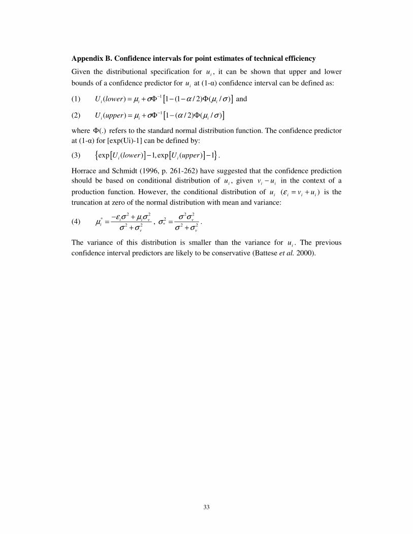
33

Appendix B. Confidence intervals for point estimates of technical efficiency

Given the distributional specification for iu , it can be shown that upper and lower bounds of a confidence predictor for iu at (1-�) confidence interval can be defined as:

(1) [ ]1( ) 1 (1 / 2) ( / )i i iU lower µ σ α µ σ−= + Φ − − Φ and

(2) [ ]1( ) 1 ( / 2) ( / )i i iU upper µ σ α µ σ−= + Φ − Φ

where (.)Φ refers to the standard normal distribution function. The confidence predictor at (1-�) for [exp(Ui)-1] can be defined by:

(3) [ ]{ [ ] }exp ( ) 1,exp ( ) 1i iU lower U upper− − .

Horrace and Schmidt (1996, p. 261-262) have suggested that the confidence prediction should be based on conditional distribution of iu , given ii uv − in the context of a production function. However, the conditional distribution of iu )( iii uv +=ε is the truncation at zero of the normal distribution with mean and variance:

(4) 2 2

*2 2

i i vi

v

ε σ µ σµσ σ

− +=+

, 2 2

2* 2 2

v

v

σ σσσ σ

=+

.

The variance of this distribution is smaller than the variance for iu . The previous confidence interval predictors are likely to be conservative (Battese et al. 2000).

34

Appendix C. Bootstrap procedure for dominance rankings

Let 1X and 2X be two variables (such as efficiency in production) at either two different points in time or for different attributes like regional location. Let kiX , i = 1,

..., N; k = 1, 2 denote the not necessarily i.i.d. observations. Let 1U denote the class of all von Neumann-Morgenstern type utility functions, u, such that 0≥′u , (increasing). Also, let 2U denote the class of all utility functions in 1U for which 0≤′′u (strict concavity). Let )1( pX and )2( pX denote the p-th quantiles, and )(1 xF and )(2 xF denote the cumulative distribution functions, respectively. Following the notation in Maasoumi and Heshmati (2004) the first and second order SD are defied as follows.

1X First Order Stochastic Dominates 2X , denoted 21 XFSDX , if any of the following equivalent conditions holds:

(1) [ ] [ ])()( 21 XuEXuE ≥ for all 1Uu ∈ , with strict inequality for some u; or

(2) )()( 21 xFxF ≤ for all x with strict inequality for some x; or

(3) )2()1( pp XX ≥ for all 10 ≤≤ p , with strict inequality for some p.

1X Second Order Stochastic Dominates 2X , denoted 21 XSSDX , if any of the following equivalent conditions holds:

(4) [ ] [ ])()( 21 XuEXuE ≥ for all 2Uu ∈ , with strict inequality for some u; or

(5) � �≤∞− ∞−

x x

dttFdttF )()( 21 for all x with strict inequality for some x; or

(6) � �=Φ≥=Φp p

tt dtXpdtXp0 0

)2(2)1(1 )()( for all 10 ≤≤ p , with strict inequality for

some value(s) p.

Weak orders of SD are obtained by eliminating the requirement of strict inequality at some point. When these conditions are not met, as when Generalized Lorenz Curves of two distributions cross, unambiguous First and Second order SD is not possible. Any strong ordering by specific indices that correspond to the utility functions 1U and 2U classes, will not enjoy general consensus.

This approach fixes the critical value (zero) at the boundary of our null, and estimates the associated significance level by bootstrapping the sample or its blocks. This renders our tests asymptotically similar and unbiased on the boundary. This is similar in spirit to inference based on p-values. This method could also be used to compare the two distributions up to any desired quantile, for instance, for performance rankings. The test statistics are as follows.

Suppose that there are 2 prospects 1X , 2X and let { }2,1: == kXA k . Let { }NiX ki ,...,2,1: = be realizations of kX for k=1,2. Let ),( 21 xxF be the joint c.d.f. of

),( 21 ′XX . Now define the following functionals of the joint distribution:

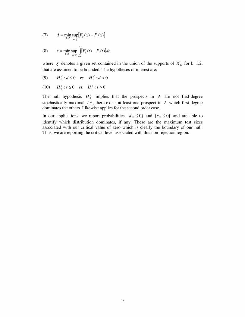
35

(7) [ ])()(supmin xFxFd lkxlk

−=∈≠ χ

(8) [ ]�∞−∈≠

−=x

lkxlk

dttFtFs )()(supminχ

where χ denotes a given set contained in the union of the supports of kiX for k=1,2, that are assumed to be bounded. The hypotheses of interest are:

(9) 0:.0: 10 >≤ dHvsdH dd

(10) 0:.0: 10 >≤ sHvssH ss

The null hypothesis dH 0 implies that the prospects in A are not first-degree stochastically maximal, i.e., there exists at least one prospect in A which first-degree dominates the others. Likewise applies for the second order case.

In our applications, we report probabilities }0{ ≤Nd and }0{ ≤Ns and are able to identify which distribution dominates, if any. These are the maximum test sizes associated with our critical value of zero which is clearly the boundary of our null. Thus, we are reporting the critical level associated with this non-rejection region.

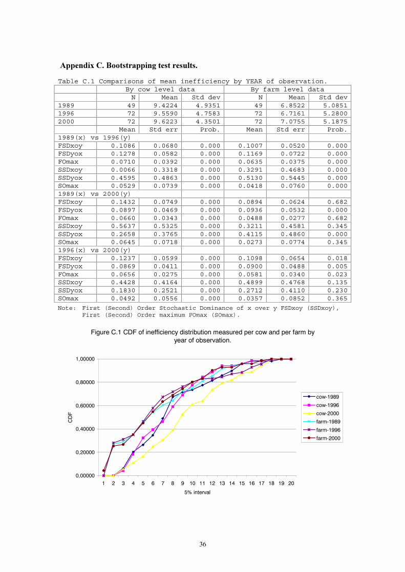
36

�������������� � �������� �� ������ �� Table C.1 Comparisons of mean inefficiency by YEAR of observation. By cow level data By farm level data N Mean Std dev N Mean Std dev 1989 49 9.4224 4.9351 49 6.8522 5.0851 1996 72 9.5590 4.7583 72 6.7161 5.2800 2000 72 9.6223 4.3501 72 7.0755 5.1875 Mean Std err Prob. Mean Std err Prob. 1989(x) vs 1996(y) FSDxoy 0.1086 0.0680 0.000 0.1007 0.0520 0.000 FSDyox 0.1278 0.0582 0.000 0.1169 0.0722 0.000 FOmax 0.0710 0.0392 0.000 0.0635 0.0375 0.000 SSDxoy 0.0066 0.3318 0.000 0.3291 0.4683 0.000 SSDyox 0.4595 0.4863 0.000 0.5130 0.5445 0.000 SOmax 0.0529 0.0739 0.000 0.0418 0.0760 0.000 1989(x) vs 2000(y) FSDxoy 0.1432 0.0749 0.000 0.0894 0.0624 0.682 FSDyox 0.0897 0.0469 0.000 0.0936 0.0532 0.000 FOmax 0.0660 0.0343 0.000 0.0488 0.0277 0.682 SSDxoy 0.5637 0.5325 0.000 0.3211 0.4581 0.345 SSDyox 0.2658 0.3765 0.000 0.4115 0.4860 0.000 SOmax 0.0645 0.0718 0.000 0.0273 0.0774 0.345 1996(x) vs 2000(y) FSDxoy 0.1237 0.0599 0.000 0.1098 0.0654 0.018 FSDyox 0.0869 0.0411 0.000 0.0900 0.0488 0.005 FOmax 0.0656 0.0275 0.000 0.0581 0.0340 0.023 SSDxoy 0.4428 0.4164 0.000 0.4899 0.4768 0.135 SSDyox 0.1830 0.2521 0.000 0.2712 0.4110 0.230 SOmax 0.0492 0.0556 0.000 0.0357 0.0852 0.365

Note: First (Second) Order Stochastic Dominance of x over y FSDxoy (SSDxoy), First (Second) Order maximum FOmax (SOmax).

Figure C.1 CDF of inefficiency distribution measured per cow and per farm by year of observation.

0,00000

0,20000

0,40000

0,60000

0,80000

1,00000

1 2 3 4 5 6 7 8 9 10 11 12 13 14 15 16 17 18 19 20

5% interval

CD

F

cow-1989

cow-1996

cow-2000

farm-1989

farm-1996

farm-2000

37

Table C.2 Comparisons of mean inefficiency by SIZE of farm. By cow level data By farm level data N Mean Std dev N Mean Std dev Small 175 10.2261 4.5852 175 11.6541 5.2507 Medium 418 9.0995 4.9756 418 7.4849 4.1227 Large 219 10.2224 5.8792 219 1.3921 0.3123 Mean Std err Prob. Mean Std err Prob. Small(x) vs Medium(y) FSDxoy 0.0137 0.0096 0.000 0.0001 0.0001 0.000 FSDyox 0.1310 0.0369 0.000 0.4321 0.0317 0.000 FOmax 0.0137 0.0094 0.000 0.0001 0.0001 0.000 SSDxoy 0.0066 0.0084 0.000 0.0000 0.0000 0.000 SSDyox 0.5176 0.1816 0.000 2.8071 0.2985 0.000 SOmax 0.0063 0.0066 0.000 0.0000 0.0000 0.000 Small(x) vs Large(y) FSDxoy 0.0571 0.0259 0.000 -0.0056 0.0060 0.682 FSDyox 0.1073 0.0386 0.000 0.9975 0.0031 0.000 FOmax 0.0509 0.0205 0.000 -0.0056 0.0060 0.682 SSDxoy 0.0721 0.1332 0.000 -0.4851 0.0336 1.000 SSDyox 0.3576 0.2040 0.000 7.9609 0.3086 0.000 SOmax 0.0331 0.0544 0.000 -0.4851 0.0336 1.000 Medium(x) vs Large(y) FSDxoy 0.0969 0.0310 0.000 -0.0001 0.0001 0.344 FSDyox 0.0081 0.0136 0.000 0.9779 0.0072 0.000 FOmax 0.0078 0.0126 0.000 -0.0001 0.0001 0.344 SSDxoy 0.5368 0.2107 0.000 -0.7818 0.0285 1.000 SSDyox 0.0070 0.0178 0.000 3.9517 0.1235 0.000 SOmax 0.0065 0.0156 0.000 -0.7818 0.0285 1.000

Note: First (Second) Order Stochastic Dominance of x over y FSDxoy (SSDxoy), First (Second) Order maximum FOmax (SOmax).

Figure C.2 CDF of inefficiency distribution measured per cow and per farm by size of farm.

0,00000

0,20000

0,40000

0,60000

0,80000

1,00000

1 2 3 4 5 6 7 8 9 10 11 12 13 14 15 16 17 18 19 20

5% interval

CD

F

cow-small

cow-medium

cow-large

farm-small

farm-medium

farm-large

38

Table C.3 Comparisons of mean inefficiency by REGION of location. By cow level data By farm level data N Mean Std dev N Mean Std dev South 100 10.4491 5.6848 100 6.5060 4.1221 Central 505 8.4355 4.4701 505 4.7109 2.8871 North 207 12.2077 5.5479 207 11.8041 6.7376 Mean Std err Prob. Mean Std err Prob. South(x) vs Central(y) FSDxoy 0.0067 0.0073 0.000 0.0055 0.0147 0.000 FSDyox 0.1857 0.0454 0.000 0.2293 0.0480 0.000 FOmax 0.0067 0.0073 0.000 0.0055 0.0147 0.000 SSDxoy 0.0022 0.0077 0.000 0.0117 0.0343 0.000 SSDyox 1.1596 0.3367 0.000 1.9254 0.4957 0.000 SOmax 0.0022 0.0077 0.000 0.0117 0.0343 0.000 South(x) vs North(y) FSDxoy 0.2707 0.0554 0.000 0.4668 0.0445 0.000 FSDyox 0.0290 0.0285 0.000 0.0182 0.0280 0.280 FOmax 0.0289 0.0282 0.000 0.0182 0.0280 0.000 SSDxoy 0.7818 0.2480 0.000 3.3718 0.3813 0.000 SSDyox 0.0016 0.0169 0.000 -0.1971 0.0661 0.993 SOmax 0.0015 0.0148 0.000 -0.1971 0.0661 0.993 Central(x) vs North(y) FSDxoy 0.3729 0.0376 0.000 0.6299 0.0033 0.000 FSDyox 0.0052 0.0034 0.025 0.0002 0.0022 0.507 FOmax 0.0052 0.034 0.025 0.0002 0.0022 0.507 SSDxoy 1.6826 0.1784 0.000 4.5354 0.2936 0.000 SSDyox -0.0019 0.0019 0.645 -0.2562 0.0232 1.000 SOmax -0.0019 0.0019 0.645 -0.2562 0.0232 1.000

Note: First (Second) Order Stochastic Dominance of x over y FSDxoy (SSDxoy), First (Second) Order maximum FOmax (SOmax).

Figure C.3 CDF of inefficiency distrubution measured per cow and per farm by reginal location.

0,00000

0,20000

0,40000

0,60000

0,80000

1,00000

1 2 3 4 5 6 7 8 9 10 11 12 13 14 15 16 17 18 19 20

5% interval

CD

F

cow-south

cow-middle

cow-nroth

farm-south

farm-middle

farm-north

39

Table C.4 Comparisons of mean inefficiency by CAPITAL intensity. By cow level data By farm level data N Mean Std dev N Mean Std dev Low 200 7.6609 3.9661 200 6.0557 4.4543 Medium 408 9.9455 4.8794 408 6.9657 5.6354 High 204 10.9897 6.1828 204 6.9604 5.2660 Mean Std err Prob. Mean Std err Prob. Low(x) vs Medium(y) FSDxoy 0.2590 0.0399 0.000 0.1070 0.0315 0.000 FSDyox 0.0004 0.0021 0.000 0.0450 0.0325 0.052 FOmax 0.0004 0.0021 0.000 0.0414 0.0271 0.052 SSDxoy 1.5225 0.2490 0.000 0.6586 0.3250 0.020 SSDyox 0.0000 0.0000 0.000 0.0482 0.0809 0.268 SOmax 0.0000 0.0000 0.000 0.0355 0.0590 0.288 Low(x) vs High(y) FSDxoy 0.2680 0.0449 0.000 0.1417 0.0490 0.000 FSDyox 0.0001 0.0001 0.240 0.0264 0.0254 0.113 FOmax 0.0001 0.0001 0.240 0.0249 0.0230 0.113 SSDxoy 1.4002 0.2269 0.000 0.4639 0.2785 0.039 SSDyox -0.0052 0.050 0.649 0.0142 0.0775 0.506 SOmax -0.0052 0.0050 0.649 -0.0026 0.0451 0.545 Medium(x) vs High(y) FSDxoy 0.0813 0.0263 0.000 0.0683 0.0360 0.004 FSDyox 0.0288 0.0288 0.000 0.0626 0.0237 0.000 FOmax 0.0248 0.0224 0.000 0.0453 0.0204 0.004 SSDxoy 0.3879 0.2022 0.000 0.1755 0.1463 0.103 SSDyox 0.0111 0.0297 0.000 0.1771 0.2083 0.283 SOmax 0.0085 0.0209 0.000 0.0387 0.0785 0.386

Note: First (Second) Order Stochastic Dominance of x over y FSDxoy (SSDxoy), First (Second) Order maximum FOmax (SOmax).

Figure C.4 CDF of inefficiency distribution measured per cow and per farm by capital intensity.

0,00000

0,20000

0,40000

0,60000

0,80000

1,00000

1 2 3 4 5 6 7 8 9 10 11 12 13 14 15 16 17 18 19 20

5% interval

CD

F

cow-cap-low

cow-cap-medium

cow-cap-high

farm-cap-low

farm-cap-medium

farm-cap-high

40

Table C.5 Comparisons of mean inefficiency by LABOUR intensity. By cow level data By farm level data N Mean Std dev N Mean Std dev Low 208 7.7976 3.8448 208 4.6145 4.9879 Medium 393 9.5624 4.9594 393 6.6247 4.6924 High 211 11.6203 5.9905 211 9.0508 5.6797 Mean Std err Prob. Mean Std err Prob. Low(x) vs Medium(y) FSDxoy 0.1682 0.0387 0.000 0.3355 0.0401 0.000 FSDyox 0.0043 0.0059 0.000 0.0242 0.0153 0.008 FOmax 0.0043 0.0059 0.000 0.0242 0.0153 0.008 SSDxoy 1.2452 0.2735 0.000 1.7167 0.3012 0.000 SSDyox 0.0046 0.0067 0.000 -0.1618 0.0328 1.000 SOmax 0.0046 0.0067 0.000 -0.1618 0.0328 1.000 Low(x) vs High(y) FSDxoy 0.3204 0.0401 0.000 0.5113 0.0427 0.000 FSDyox 0.0001 0.0001 0.000 0.0010 0.0034 0.171 FOmax 0.0001 0.0001 0.000 0.0010 0.0034 0.171 SSDxoy 1.6903 0.2154 0.000 2.7761 0.3279 0.000 SSDyox 0.0000 0.0000 0.000 -0.3510 0.0387 1.000 SOmax 0.0000 0.0000 0.000 -0.3510 0.0387 1.000 Medium(x) vs High(y) FSDxoy 0.1774 0.0355 0.000 0.2403 0.0395 0.000 FSDyox 0.0102 0.0143 0.096 0.0007 0.0028 0.276 FOmax 0.0102 0.0143 0.096 0.0007 0.0028 0.276 SSDxoy 0.8244 0.1984 0.000 1.4350 0.2770 0.000 SSDyox -0.0026 0.0025 0.650 -0.0813 0.0275 0.999 SOmax -0.0026 0.0025 0.650 -0.0813 0.0275 0.999

Note: First (Second) Order Stochastic Dominance of x over y FSDxoy (SSDxoy), First (Second) Order maximum FOmax (SOmax).

Figure C.5 CDF of inefficiency distribution measured as per cow and per farm by labor intensity.

0,00000

0,20000

0,40000

0,60000

0,80000

1,00000

1 2 3 4 5 6 7 8 9 10 11 12 13 14 15 16 17 18 19 20

5% interval

CD

F

cow-lab-low

cow-lab-medium

cow-lab-high

farm-lab-low

farm-lab-medium

farm-lab-high

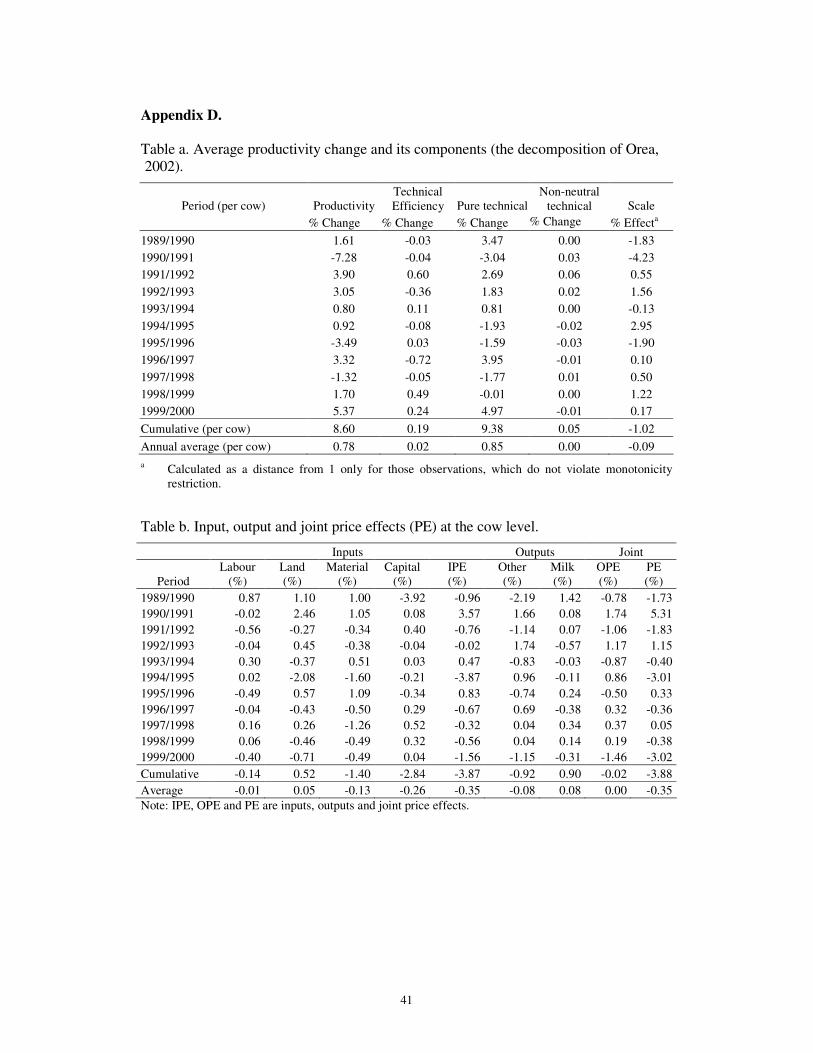
41

Appendix D. Table a. Average productivity change and its components (the decomposition of Orea, 2002).

Period (per cow) Productivity Technical Efficiency Pure technical

Non-neutral technical Scale

% Change % Change % Change % Change % Effecta 1989/1990 1.61 -0.03 3.47 0.00 -1.83 1990/1991 -7.28 -0.04 -3.04 0.03 -4.23 1991/1992 3.90 0.60 2.69 0.06 0.55 1992/1993 3.05 -0.36 1.83 0.02 1.56 1993/1994 0.80 0.11 0.81 0.00 -0.13 1994/1995 0.92 -0.08 -1.93 -0.02 2.95 1995/1996 -3.49 0.03 -1.59 -0.03 -1.90 1996/1997 3.32 -0.72 3.95 -0.01 0.10 1997/1998 -1.32 -0.05 -1.77 0.01 0.50 1998/1999 1.70 0.49 -0.01 0.00 1.22 1999/2000 5.37 0.24 4.97 -0.01 0.17 Cumulative (per cow) 8.60 0.19 9.38 0.05 -1.02 Annual average (per cow) 0.78 0.02 0.85 0.00 -0.09 a Calculated as a distance from 1 only for those observations, which do not violate monotonicity

restriction.

Table b. Input, output and joint price effects (PE) at the cow level.

Inputs Outputs Joint

Period Labour

(%) Land (%)

Material (%)

Capital (%)

IPE (%)

Other (%)

Milk (%)

OPE (%)

PE (%)

1989/1990 0.87 1.10 1.00 -3.92 -0.96 -2.19 1.42 -0.78 -1.73 1990/1991 -0.02 2.46 1.05 0.08 3.57 1.66 0.08 1.74 5.31 1991/1992 -0.56 -0.27 -0.34 0.40 -0.76 -1.14 0.07 -1.06 -1.83 1992/1993 -0.04 0.45 -0.38 -0.04 -0.02 1.74 -0.57 1.17 1.15 1993/1994 0.30 -0.37 0.51 0.03 0.47 -0.83 -0.03 -0.87 -0.40 1994/1995 0.02 -2.08 -1.60 -0.21 -3.87 0.96 -0.11 0.86 -3.01 1995/1996 -0.49 0.57 1.09 -0.34 0.83 -0.74 0.24 -0.50 0.33 1996/1997 -0.04 -0.43 -0.50 0.29 -0.67 0.69 -0.38 0.32 -0.36 1997/1998 0.16 0.26 -1.26 0.52 -0.32 0.04 0.34 0.37 0.05 1998/1999 0.06 -0.46 -0.49 0.32 -0.56 0.04 0.14 0.19 -0.38 1999/2000 -0.40 -0.71 -0.49 0.04 -1.56 -1.15 -0.31 -1.46 -3.02 Cumulative -0.14 0.52 -1.40 -2.84 -3.87 -0.92 0.90 -0.02 -3.88 Average -0.01 0.05 -0.13 -0.26 -0.35 -0.08 0.08 0.00 -0.35 Note: IPE, OPE and PE are inputs, outputs and joint price effects.