sio 230 geophysical inverse theory 2009 supplementary notes 1
TRANSCRIPT
SIO 230 Geophysical Inverse Theory 2009
Supplementary Notes
1. Introduction
In geophysics we are often faced with the following situation. We have
measurements made at the surface of the Earth of some quantity, like the
magnetic field, or some seismic waveforms, and we want to know some
property of the ground under the place where the data were measure.
Furthermore, the physics is well understood, and if the property we are
seeking were accurately known, we would be able to reconstruct quite
accurately the observations that we have taken. Now we wish to infer the
unknown property from the measurements. This is the typical geophysi-
cal inverse problem. It is called an inverse problem, because it reverses
the process of predicting the values of the measurements, which is called
the forward problem. The inverse problem is always more difficult than
the forward problem; in fact we have to assume that the forward problem
is completely under control before we can even begin to think about the
inverse problem, and of course there are plenty of geophysical systems
where the forward problem is still incompletely understood, such as in the
geodynamo problem, or the problem of earthquake fault dynamics.
Why is the inverse problem more difficult? There are mathematical
reasons why recovering unknown functions that appear as factors in dif-
ferential equations is a complicated business, but the practical issue is
less esoteric: the measurements are finite in number and of limited preci-
sion, but the unknown property is a function of position, and requires in
principle infinitely many parameters to describe it. We are always faced
with the problem of nonuniqueness: more than one solution can reproduce
the data in hand. What can we do?
The most obvious response is to artificially complete the data, by
interpolating, filling in the gaps somehow. Then in some circumstances it
may be possible to prove a uniqueness theorem, which states that only
one model corresponds to each complete data set. When this can be done
(which may be hard) you might think the difficulties have been conquered,
but that turns out not to be true. Most geophysical inverse problems are
ill-posed in the sense that they are unstable: then an infinitesimal pertur-
bation of a special kind in the data can result in a finite change in the
model. As a consequence the details of the interpolation process used to
complete the data are not irrelevant details as one would wish, but they
can control gross features of the answer, in contrast to the forward prob-
lem, where it is invariably the case that the solution is not only unique, it
is stable too.
Another strategy, more commonly used in the past before the advent
of larger computers, is to drastically oversimplify the model, for example,

-2-
by claiming the unknown structure consists of a small number of layers or
zones within which the unknown property is uniform. If there are good
geological reasons for doing this, it is still a viable option, but when there
is no evidence for this arrangement, even if the simplified model can be
made to match the data (and usually it cannot), the inherent nonunique-
ness means we are uncertain of the significance of our solution. None-the-
less geometrical simplification is powerful tool, and often it is the only
wa y to extract useful information. For example, reduction of two- or
three-dimensional variations to one dimension may often be a reasonable
approximation. The major features of a system can be captured by the
assumption that the property varies only with depth, or radius in a spher-
ical Earth, or horizontally.
Clearly if we assume, for example, that electrical conductivity varies
only with depth, we are looking for a simple model. The next strategy
takes the idea of seeking simplicity explicit while allowing as much com-
plexity as necessary: this is called regularization. Here, instead of simpli-
fying the model by reducing its degrees of freedom, we ask for the sim-
plest model consistent with observation. Obviously simplicity can be
defined in various ways, but as we will see, the idea is usually to reduce
the wiggliness, or roughness in the solution as far as possible. Unstable
problems manifest themselves by the introduction of short wavelength
oscillations, often of large amplitude, that are not required by the data,
but appear because of minor imperfections in the measurements or even
because of numerical round-off in the finite-precision computer calcula-
tions. By choosing from among the family of models the one with the least
roughness, we avoid as far as possible being deceived that there are
‘‘interesting’’ features in the ground, that are in fact accidental. Regular-
ization is today a completely commonplace strategy in inverse theory.
But even after we have obtained the ‘‘simplest possible’’ model by
regularization, what do we know with certainty about the Earth? Geo-
physicists are lamentably quick to assume that the properties of the regu-
larized solution are properties of the true Earth, but that is not guaran-
teed. If we want to be mathematically rigorous, not a lot is known about
the question except for the so-called linear inverse problems. For mea-
surements of a single number, we expect to be able to assign an uncer-
tainty, usually an estimate of the standard error derived from statistics:
for example, a = 6371. 01 ± 0. 02 km. Why can’t we just assign a similar
uncertainty to the solution at every point in the model? That seems very
reasonable, at first. But, unless we are willing to make other assumptions
about the model, assumptions not contained in the measurements, such
uncertainties cannot be derived from the data. The reason for this is that
it is always possible for a very thin layer to be present, with huge con-
trasts in value, without making an observable perturbation to the obser-
vations. Such a model is therefore consistent with the data, and is in the
set of all solutions to the inverse problem. At any point, the allowed devi-
ations can be arbitrarily large and so we cannot (from the measurements
-3-
alone) ascribe a point-wise uncertainty.
One solution to this dilemma is to say we are never interested in the
model value at a point, only its average value over some region. This is a
practical matter: in well logs we see large oscillations in properties that
we could never expect to match with models based on surface measure-
ments like seismics or magnetics, and so we are always content if the seis-
mic model matches a smoothed version of the well-log record. The uncer-
tainty in a solution may be limited if we specify an averaging scale. That
is the basis for the resolution available in a solution, something we will
spend some time on. Averaging over a scale can be useful in its own right
and even applies to nonlinear problems; see Medin, Parker, and Consta-
ble, 2007. Another idea, hinted at already, is to assume some reasonable
model property as an additional constraint. For example, if we can plausi-
bly assert that conductivity must increase with depth because of increas-
ing temperature, then that eliminates the very possibility of a thin layer;
with this assumption point-wise uncertainties can be computed. See
Stark and Parker, 1987. Another popular assumption (but not my
favorite) is to assign a probabilistic framework to the problem: in my opin-
ion too much must be assumed (such as Gaussian statistics and a known
autocovariance function) without any real justification.
A word on notation. Equations of these Supplementary Notes begin
anew at (1) in each numbered section. When I refer to equation outside
the current section I will use the form 5(2), which means section 5, equa-
tion number (2). When I refer to an equation Geophysical Inverse Theory
(GIT), I will use the form 2.05(13), which means section 2.05 in Chapter 2,
equation (13).
References
Medin, A. E., Parker, R. L., and Constable, S., Making sounding infer-
ences from geomagnetic sounding, PEPI, 160, 51-9, 2007.
Parker, R. L., Geophysical Inverse Theory, Princeton Univ, Press, 1994.
Stark, P. B. and Parker, R. L., Velocity bounds from statistical estimates of
τ ( p) and X ( p), J. Geophys. Res., 92, 2713-9, 1987.

-4-
2. An Illustration
To give you an idea of the sort of thing we will encounter, here is a seem-
ingly simple, and to some familiar, geophysical problem that has attracted
the attention of marine geologists and geophysicists for 40 years. A
seamount is a marine volcano, which can be formed at a ridge or in the
middle of a plate. Most seamounts are strongly magnetic, and they pro-
duce a magnetic anomaly at the sea surface that is easy to observe. A
seamount is depicted below in Figure 2.1, and its magnetic anomaly is
shown schematically in Figure 2.2. We would like to deduce the internal
magnetization vector for the seamount, and in particular the direction of
magnetization, because this vector gives paleomagnetic information about
the motion of the plate since the time of formation of the volcano − most
seamounts form quickly, so the magnetization vector can be used as a
kind of snapshot of the paleomagnetic latitude.
Let us first solve the forward problem. The magnetic anomaly is the
magnetic field remaining after the main geomagnetic field has been
removed, which can be done fairly accurately using satellite models of the
longest wavelength fields. The magnetic field due to the seamount is
Figure 2.1: Model bathymetry of seamount LR148.8W (48.2°S, 148.8°
W). Each square in the base is 5 km on a side and the arrow points
north.
-5-
given by
∆B(r) =V
∫ G(s, r) ⋅ M(s) d3s (1)
where M is the magnetization vector at the point s within the seamount
V and the vector valued function G is given by
G(s, r) =µ0
4πB0 ⋅ ∇ ∇
1
|r − s|(2)
where ∇ acts on s, and B0 is a known constant unit vector and
µ0 = 4π ×10−7Hm−1 = 100 nT m A−1 the permittivity of free space in SI
units. All the grad operators here act on the coordinate s. Equations
(1)-(2) just state that the observed field at r is the sum of the fields from
all the elementary dipoles within V . If we knew M, which is just the den-
sity of dipole moments, we could compute ∆B from (1) and (2), which
means the forward problem has been solved.
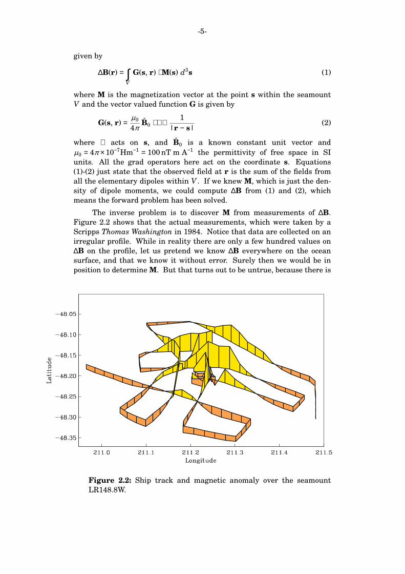
The inverse problem is to discover M from measurements of ∆B.
Figure 2.2 shows that the actual measurements, which were taken by a
Scripps Thomas Washington in 1984. Notice that data are collected on an
irregular profile. While in reality there are only a few hundred values on
∆B on the profile, let us pretend we know ∆B everywhere on the ocean
surface, and that we know it without error. Surely then we would be in
position to determine M. But that turns out to be untrue, because there is
Figure 2.2: Ship track and magnetic anomaly over the seamount
LR148.8W.

-6-
no uniqueness theorem for this inverse problem, even when perfect data
like these are available. We demonstrate the nonuniqueness with some
simple vector calculus. First rewrite (1) as
∆B(r) =V
∫ ∇ g ⋅ M(s) d3s (3)
where
g(s, r) =µ0
4πB0 ⋅ ∇
1
|r − s|(4)
which is OK because B0 is constant. Next consider a magnetization vec-
tor inside V given by m = ∇ f where f is some smooth function. Then (3)
becomes
∆B(r) =V
∫ ∇ g ⋅ ∇ f d3s (5)
=V
∫ [∇ ⋅ ( f ∇ g) − f ∇ 2 g] d3s (6)
where I have used the very useful vector identity:
∇ ⋅ ( f V) = ∇ f ⋅ V + f ∇ ⋅ V. But it is easily seen that ∇ 2 g = 0: it is the
Laplacian of 1/R, the potential of a point charge, which vanishes except at
the point r; since the observation site is never inside V , it follows that the
second term in the integral in (6) vanishes. Next we apply Gauss’s Diver-
gence Theorem to the other term:
∆B(r) =V
∫ ∇ ⋅ ( f ∇ g) d3s =∂V
∫ f n ⋅ ∇ g d2s (7)
where n is the outward facing normal to the volume V , and ∂V denotes
the surface of V . Suppose now I choose any smooth function f (s) that
vanishes on ∂V . We see from (7) that the magnetic anomaly ∆B due to a
magnetization m = ∇ f vanishes identically outside V .
The consequences of this result are that whatever the true magneti-
zation Mtrue may be, I can add a magnetization function like m to it to
form
M = Mtrue + m (8)
and the new magnetization distribution will match the data just as well
as Mtrue. From (1):
∆B =V
∫ [G ⋅ [Mtrue + m] d3s (9)
=V
∫ G ⋅ Mtrued3s +V
∫ G ⋅ m d3s =V
∫ G ⋅ Mtrued3s +V
∫ G ⋅ ∇ f d3s (10)

-7-
=V
∫ G ⋅ Mtrued3s + 0 . (11)
Thus, from the field observations, there is no way to distinguish between
the true magnetization and any member of an infinitely large family of
alternatives. The magnetization inverse problem does not have a unique
solution even with perfect data. The magnetization m is called, rather
dramatically, a magnetic annihilator for this problem.
The first answer to the dilemma of nonuniqueness was the Drastic
Simplification strategy, introduced for the seamount problem in 1962
(Vacquier, 1962), and still in widespread use today! It is simply asserted
that within V the magnetization is uniform, in other words, M(s) is not a
function of position at all, but a constant vector. Then there are exactly
three unknowns, the x, y and z components, instead of infinitely many,
quite a reduction. In the 1960s there was no compelling evidence to con-
tradict this simple model, but now we know it is wide of the mark. As
various seamounts were surveyed magnetically it quickly became clear
that the uniform magnetization model was incapable of matching the
data, but as I said, people continue to use it to infer paleopoles to this day.
Regularization in this problem (Parker, et al., 1987) takes the follow-
ing form. We write the magnetization distribution as the sum of two
terms:
M(s) = U + R(s) (12)
where U is a constant vector, and R varies with s; obviously any M can
written this way. To regularize the inverse problem, we ask for the model
that makes R as small as possible, in other words, we look for the most
nearly uniform model that fits the observations. Now we can always
match the measurements, and obtain a vector U for the uniform part. We
have constructed a regularized solution, the kind of thing done all the
time in seismic tomography, and surface wave inversion, and magnetotel-
luric sounding, and on and on. But how reliable is vector U, which is the
geologically significant product of the calculation? As we will see, in a lin-
ear problem like this, U is really still completely undetermined, unless we
are willing to make some further assumptions, or place additional restric-
tions on M. The information cannot come from observations of ∆B, which
as we have seen by themselves leave a huge amount of ambiguity.
There are several ways we can limit the ambiguity. One approach is
to say that we know based on samples of rocks from the seafloor and shal-
low drill holes in marine basalts that the magnitude of the magnetization
||M|| is limited in a way we would be willing to specify. In the Hilbert
space machinery that we will soon be studying, the simplest way to do
this to introduce a norm of magnetization:
||M|| = V
∫ |M(s)|2 d3s
½
. (13)
-8-
Samples would allow us to say that ||M|| ≤ m0 V with some confidence.
We will discuss how to do such calculations later in the class. While this
approach is a good idea in principle, it does not work very well for this
particular problem in practice. We find the allowed range of directions of
U is very large. And that might be the final answer; after all, it could be
that the data we have and the reasonable assumptions we might make, do
not in fact allow us to determine U accurately enough to be geologically
interesting.
But we shouldn’t give up too soon. A fact of paleomagnetism long
exploited in other problems is that rocks are magnetized with a constant
direction in large units. It would make no sense for a paleomagnetist to
take samples on the surface of an exposed unit if it was not plausible to
assume the directions are fairly uniform within. Approximate uniformity
of direction is indeed found to be the case, but not for the intensity of mag-
netization: magnetic intensity is found to vary over two or three orders of
magnitude, which is why the oversimplified model of Vacquier doesn’t
work. So we will restrict the model to be unidirectional in M; we call that
direction the unit vector M0. If the geomagnetic field reversed during the
formation of the seamount we would need both +M0 and −M0. Most
seamounts form rapidly enough that this is a low probability. With that
single assumption, unidirectionality, the inverse problem becomes a lot
harder to solve, but it turns out, it adds a lot of power to the data and
rather good results are obtained; see Parker (1991).
References
Parker, R. L., Shure, L., and Hildebrand, J., The application of inverse
theory to seamount magnetism, Rev. Geophys., 25, 17-40. 1987.
Parker, R. L., A theory of ideal bodies for seamount magnetism, J. Geo-
phys. Res., B10, 16101-12, 1991.
Vacquier, V., A machine method for computing the magnetization of a uni-
formly magnetized body from its shape and a magnetic survey, 123-37,
Benedum Earth Magnetism Symposium, Univ. Pittsburgh Press, 1962.
-9-
3. Abstract Linear Vector Spaces
This section begins a review of linear algebra and simple optimization
problems on finite-dimensional spaces. We will cover some of these prob-
lems again but in the more abstract setting of Hilbert space in Chapters
and 1 and 2 of GIT. The current segment (Section 3) is a slightly modified
version of Section 1.01 in GIT.
The definition of a linear vector space involves two types of object:
the elements of the space and the scalars. Usually the scalars will be
the real numbers but occasionally complex scalars will prove useful; we
will assume real scalars are intended unless it is specifically stated other-
wise. The elements of the space are much more diverse as we shall see in
a moment when we give a few examples. First we lay out the rules that
define a real linear vector space (‘‘real’’ because the scalars are the real
numbers): it is a set V containing elements which can be related by two
operations, addition and scalar multiplication; the operations are written
f + g and α f
where f , g ∈ V and α ∈ IR. For any f , g, h ∈ V and any scalars α and β ,
the following set of nine relations must be valid:
f + g ∈ V (1)
α f ∈ V (2)
f + g = g + f (3)
f + (g + h) = ( f + g) + h (4)
f + g = f + h, if and only if g = h (5)
α ( f + g) = α f + α g (6)
(α + β ) f = α f + β f (7)
α (β f ) = (α β ) f (8)
1 f = f . (9)
In (9) we mean that scalar multiplication by the number one results in the
same element. The notation −f means minus one times f and the rela-
tion f − g denotes f + (−g). These nine ‘‘axioms’’ are only one characteriza-
tion; other equivalent definitions are possible. Notice in (7) the meaning
of the plus sign is different on the two sides, and in (8) there are two kinds
of multiplication going on. An important consequence of these laws (so
important, some authors elevate it to axiom status and eliminate one of
the others), is that every vector space contains a unique zero element 0
with the properties that
-10-
f + 0 = f , f ∈ V
and whenever
α f = 0
either α =0 or f =0. If you have not seen it you may like to supply the
proof of this assertion.
Here are a few examples of linear vector spaces, most of which we
will come across later on. First there is the obvious space IRn. There are
two ways to think about this space. One is simply as an ordered n-tuples
of real numbers. So an element x ∈ IRn is just
x = (x1, x2, . . . , xn) (10)
where x j ∈ IR. The definition of addition of two vectors and multiplication
by a scalar is self-evident, and if we check off the list of axioms, they are
all very obviously true for this collection of elements. The alternative way
of looking at IRn is as the set of column vectors:
x =
x1
x2
:
xn
. (11)
This form highlights the fact that IRn is really a special case of one of the
spaces of real matrices, IRm × n; in fact, to use the form (11) we should
write the space as IRn×1.
This brings to the space of real matrices IRm × n. As you could easily
guess, it is the collection of all real rectangular arrays of real numbers in
the form:
A =
a11
a21
:
am1
a12
a22
:
am2
. . .
. . .
. . .
. . .
a1n
a2n
:
amn
. (12)
Once again it is clear what it means to add two matrices of the same size,
and multiplication by a scalar simply means every entry is multiplied by
that number. We will be discussing matrix algebra in the next section.
Notice that I did not use the proper mathematical notation for this space
in GIT, an unfortunate oversight on my part.
Perhaps less familiar to you are spaces whose elements are not finite
sets of numbers, but functions. For example, consider the real-valued
function f that takes a real argument x restricted the closed interval
[a, b]; a mathematician would write this specification as f : [ a, b ] → IR,
and you should consider it too. The collection of all such functions that
are continuous form a space called C0[a, b]. Again, there is no difficulty in
seeing what it means to add two such functions, and that the sum of two
continuous functions is itself continuous. Scalar multiplication presents

-11-
no difficulty either, nor any of the other rules. There is a short table of
named function spaces on p 6 of GIT.
In a linear vectors space, you can always add together a collection of
elements to form a linear combination thus:
g = α 1 f1 + α 2 f2 + . . . + α k f k (13)
where f j ∈ V and the α j ∈ IR are scalars; obviously g ∈ V too. This kind
of operation is at the heart of almost everything we do in linear vector
spaces.
To a large extent all that is going on here is classification, just a way
of organizing things with names we can all agree on. But this is very use-
ful, and you must learn this language and use it.
-12-
4. Essential Linear Algebra
The next few lectures will be on linear algebra and its computational
aspects. An elementary book for much of the material is by Strang, Intro-
duction to Applied Mathematics (Wellesley-Cambridge, 1986); more
advanced and a classic in the field is Matrix Computations, 3rd Edition,
by Golub and Van Loan (Johns Hopkins Univ. Press, 1996) The program
MATLAB which you must learn for this class, manipulates matrices very
naturally.
A matrix is a rectangular array of real (or possibly complex) num-
bers arranged in sets of m rows with n entries each see 3(12); or equiva-
lently, there are n columns each m long. The set of such m by n matrices
is called IRm × n for real matrices and C| m × n for complex ones. If m =1 the
matrix is called a row vector and if n =1 it is a column vector; notice
that the space of column vectors will usually be written IRm rather than
IRm×1. The entries of the array A ∈ IRm × n are referred to by indices, aij
which means the entry on the i-th row and the j-th column. A square
matrix has m = n of course. It is customary to denote a row or column vec-
tor by a lower case letter, say x, and then the i-th element is written x j .
Here is a list of names of special matrices defined by the systematic distri-
bution of zeros in them:
Diagonal aij =0 whenever i ≠ j
Tridiagonal aij =0 whenever |i − j| > 1
Upper triangular aij =0 whenever i > j
Sparse Most entries zero
Upper triangular matrices are also called Right triangular. Lower trian-
gular matrices are defined in the analogous manner, with the inequality
reversed. Notice these definitions apply to nonsquare matrices as well as
square ones. A diagonal matrix is often conveniently written by specify-
ing its diagonal entries in order, thus:
D = diag (d1, d2, . . . dn) . (1)
In MATLAB this is D = diag(d) where d is a column or a row vector; MAT-
LAB distinguishes between column and row vectors in most circumstances,
so be careful. The square, diagonal matrix with only unity on the diago-
nal is usually denoted I (a very few authors use E) and is called the unit
matrix. In MATLAB you form the unit matrix I ∈ IRm × n by the weird
statement I = e ye(n) . Sparse matrices are very important because
they arise very frequently, and a great of work has been put into numeri-
cal algorithms for dealing with them efficiently.
As I mentioned in the previous section, the set of matrices IRm × n
forms a linear vector space under the obvious rules of addition:
A = B + C means aij = bij + cij (2)
and scalar multiplication:
-13-
B = c A means bij = c aij (3)
where A, B, C ∈ IRm × n and c ∈ IR.
Another basic manipulation, which you all know, is transposition:
B = AT means bij = a ji . (4)
Some authors and MATLAB denote transpose by A′; this is to be discour-
aged in technical writing. Transposition is just the reversal of the roles of
the columns and rows. A symmetric matrix is its own transpose:
AT = A; it is obviously square.
Most important is matrix multiplication (IRm×n × IRn×p → IRm×p):
C = A B means cij =n
k=1Σ aik bkj . (5)
Notice that you can only multiply two matrices when the numbers of col-
umns in the first one equals the number of rows in the second; but the
other dimensions are not important, so nonsquare matrices can be multi-
plied. The combination of the operations of addition and matrix multipli-
cation allows one to define matrix arithmetic analogous to real number
arithmetic. The standard arithmetic law of distribution is valid:
A(B + C) = AB + AC. Less obviously, association of multiplication holds:
A (B C) = (A B) C, when the orders of the matrices are the correct size to
permit the product. So we get used to doing algebra on matrices as if they
were numbers, but multiplication is not commutative. This means in
general the order of multiplication matters, that is:
A B ≠ B A (6)
unless some special property exists.
When one multiplies a matrix into a column vector, there are a num-
ber of useful ways of interpreting this operation:
y = A x . (7)
If the vectors x and y are in the same space, Rm one can view A as pro-
viding a linear mapping or linear transformation of one vector into
another. This is especially valuable for 3-vectors and then A represents
the components of a tensor (referred to a particular frame). For example,
x might be angular velocity about some point, A the inertia tensor, and y
would be the angular momentum about the point; or x could be magnetiz-
ing magnetic field, A the susceptibility tensor, and y the resultant magne-
tization vector in a specimen. Another linear transformation performed
by matrices in ordinary space is rigid body rotation, used in plate-tectonic
reconstruction, and space-ship animation and CAD applications; this
involves a special square nonsymmetric matrix to be defined later.
Another useful perspective on matrix multiplication is supplied by
thinking about A as the ordered collection of its columns as column vec-
tors:
-14-
y = A x = [a1, a2, . . . an] x = x1a1 + x1a2 + . . . + xnan (8)
so that the new vector is just a linear combination of the column vectors of
A with coefficients given by the elements of x. This is the way we typi-
cally think about matrix multiplication when it applies to fitting a model:
here y contains data values, the columns of A are the predictions of a the-
ory that includes unknown weight factor given by the entries in x.
We can interpret matrix multiplication this way too. Now let the col-
umns of B be the focus; then
A B = A [b1, b2, . . . bp] = [A b1, A b2, . . . A bp] . (9)
In other words, A simply transforms the column vectors of B one at a
time. As a matter of fact, it is useful sometimes to partition a large
matrix into a set of rectangular submatrices or blocks. Then if you have
two matrices, both partitioned into blocks in a consistent manner, you can
multiply them together, treating the blocks just as if they were numbers.
There are two ways of multiplying two vectors. The outer product
if x ∈ IRp and y ∈ IRq :
x yT =
x1 y1
.
x p y1
. . .
.
. . .
x1 yq
.
x p yq
∈ IRp×q . (10)
And the inner product of two column vectors of the same length:
xT y = x1 y1 + x2 y2 +. . . + xn yn = yT x . (11)
Of course the inner product is just the vector dot product of vector anal-
ysis. Notice that if we write A and B as column vectors:
A = [a1, a2, . . . am] and B = [b1, b2, . . . bn] (12)
then the matrix product C = AT B is by definition (5) a collection of inner
products:
c jk = aTj bk, j =1, 2 . . . m, k =1, 2, . . . n (13)
The unit matrix I is special for matrix multiplication. Whenever the
product I A is permitted, the matrix A is unchanged; the unit matrix
plays the role of the number one in arithmetic. Also if A is square and if
there is a matrix B so that A B = I, the matrix B is called the inverse of
A and is written A−1. When it exists, the inverse matrix is unique.
Square matrices A that possess no inverse are called singular; when the
inverse exists, A is called nonsingular. The inverse of the transpose of
A is the transpose of the inverse:
(AT )−1 = (A−1)T (14)
and sometimes authors write (A−1)T = A−T . I don’t like this notation,
however, and so I will never use it.
-15-
The idea of the inverse is supposed to be useful for solving linear
systems of algebraic equations. When we write (7) and we suppose that
the vector y is known and A is square and known too, we can recover the
unknown vector x by multiplying both sides of (7) with A−1:
A−1 y = A−1 A x = I x = x . (15)
As we will see shortly, calculating the inverse and then multiplying it into
y is considered a poor way to do this numerically. How is the inverse actu-
ally calculated? We will not go into this in detail, but the ideas behind the
numerical calculation of y in (15) are important enough for us to look at
later. Once you know how to solve A x = y, it is a simple step to find A−1
from (9) setting B = I.
Two cute results. When you transpose the product of two matrices,
you can get the same result by transposing first, but you must invert the
order:
(A B)T = BT AT . (16)
And the same goes for the operation of inverting:
(A B)−1 = B−1 A−1 (17)
Exercises
4.1 Exhibit an explicit numerical example of a pair of 4 by 4 matrices
A and B that commute with each other subject to these rules: neither
of them is allowed to be diagonal and A must not be a scalar multiple
of B or its inverse. Explain the logical process that led to your
answer.
4.2 Our definition, that A B = I, strictly defines the right inverse of A.
Prove that if the left inverse exists, it is also B; that is B A = I; in
other words, prove a nonsingular matrix commutes with its inverse.
Do not assume the truth of (17). Can you prove a left inverse exists
whenever a right one does?
4.3 Show that the inverse of a nonsingular matrix is unique.
4.4 Under what conditions is the product of two symmetric matrices
also symmetric?
4.5 Prove (16) and (17).
4.6 In analysis a real self adjoint operator is a linear mapping that
satisfies (x, Ay) = (Ax, y) for every vector x, y, where (⋅, ⋅) is an inner
product. Show that for matrices and column vectors, and the inner
product (11), that from this definition A must be a symmetric matrix.
Now let us concentrate on square matrices, the kind that arise clas-
sically in the solution of linear systems. First, there is the determinant.

-16-
This is a real number that measures the "volume" of the image of a unit
cube after the matrix A has been applied to the space IRn. The value of
the determinant isn’t much use, except to tell whether it is zero, or not;
Here is one way to find it: define det (A) = a11 for A ∈ IRn × n with n =1, in
other words, a 1 ×1 matrix. For larger values of n we work up by recur-
rence:
det (A) =n
j=1Σ (−1) j+1 a1 j det (A1 j) (18)
where A1 j is the matrix in IRn−1 × n−1 found by deleting row 1 and column j
of A. A useful simple case is that of a triangular matrix: the determinant
is the product of the diagonal elements. Some other important properties
of the determinant which we will not prove:
(a) det (AB) =det (A) det (B)
(b) det (AT ) =det (A)
(c) det (A) =0, if and only if Ais singular
The determinant is used for proving theorems but in numerical work it is
seldom used.
Here are the definitions of some important kinds of square matrix.
Symmetric AT = A
Skew-symmetric AT = − A
Positive definite xT A x > 0, x ≠ 0 ∈ IRn
Positive aij > 0, all i, j
Orthogonal AT A = I
Normal AT A = A AT
Projection AT = A and A2 = A
Diagonally dominant |aii| >j≠ iΣ |aij|
The orthogonal matrix obviously has the properties that
Q−1 = QT and thus Q QT = I . (19)
Consider an orthogonal matrix Q to be composed of column vectors:
Q = [q1, q2, . . . qn] . (20)
Then the definition and (13) show that the vectors q j and qk are always
orthogonal when j ≠ k, and they are of unit Euclidean length. In other
words the columns are a collection of mutually orthogonal unit vectors.
But (19) shows that this also means the rows have exactly the same prop-
erty!
As you probably know the orthogonal matrix is the generalization of
the operation of rotation and reflection in a mirror in n-dimensional

-17-
space. We can show this in several ways. First we can easily show the
orthogonal matrix leaves the volume of an element unchanged, because
the determinant of Q is ±1. Here is the proof: From (18) or the idea that I
leaves a space unchanged, det (I) =1. But
QT Q = I . (21)
So
1 = det (QT Q) = det (Q) det (QT ) = det (Q)2 . (22)
Hence the result. A negative sign indicates the mapping Q involves
reflection, as well as rotation. But equal volume transformations aren’t
necessarily rotations. The key is that the inner product of two any vectors
is preserved.
(Qx)T (Q y) = xT QT Q y = xT (QT Q) y = xT y . (23)
When x = y this proves the length of every vector is preserved and in addi-
tion the angle between any two vectors is unchanged; so any rigid body
will be preserved in shape, which is rotation, and possible reflection.
Suppose we are in IR3 and we want to know the orthogonal matrix
for a rotation about the origin, on an axis n (a unit vector) and by an
angle θ . Then
R x = x cosθ + n n ⋅ x(1 − cosθ ) + n ××x sinθ (24)
where ×× is the ordinary vector cross product in IR3. So the elements of R
are
rij = δij cosθ + (1 − cosθ ) ni n j + sinθkΣ ε ijk n j (25)
where ε ijk is the alternator with the properties: ε ijk =0, whenever two
indices are equal; ε ijk = + 1 whenever ijk is a cyclic permutation of 123;
ε ijk = − 1 otherwise. You may find this formula useful one day.
Here is another interesting orthogonal matrix − the elementary
Householder matrix. Suppose u ∈ IRn is of unit Euclidean length,
meaning uT u =1. Then the matrix
Q = I − 2u uT (26)
is orthogonal. Proof: First note that Q is symmetric; therefore
QT Q = Q2 = (I − 2u uT ) (I − 2u uT ) (27)
= I − 4u uT + 4u uT u uT = I [QED] . (28)
So Q is both symmetric and orthogonal. (Can you think of a general spec-
ification of the class of symmetric orthogonal matrices?) The transforma-
tion of Q is quite simple to visualize as follows: Consider the vector y = Q x
= x −2u (uT x). The vector u (uT x) is the component of x lying in the u
direction. So y has that component reversed. That means x has been
-18-
reflected in the subspace normal to the direction n. (This means
det (Q) = − 1; can you prove this independently?) The reason these particu-
lar matrices are important is that they play a central role in a special
matrix factorization called QR, invented by Alston Householder in the
1950s, and the QR method solves least-squares problems; more of this
later.
Next we go over some further ideas about linear vector spaces.
First, a set of vectors {a1, a2, . . . an} in a linear vector space (for example,
IRm) is said to be linearly independent if
n
j=1Σ β j a j = 0 implies β1 = β2 = . . . = βn = 0 (29)
where β j ∈ IR. If a nontrivial linear combination of vectors can equal the
zero vector of the space, the set is called linearly dependent. A sub-
space of linear vector space is a set of vectors that is also a linear vector
space. For example, any plane in ordinary space through the origin of
coordinates; but not a plane that misses the origin. The spanning set or
more simply the span of a collection of vectors, is the linear vector space
that can be built from that collection by taking linear combinations of
them. Formally,
span {a1, a2, . . . an} = {jΣ β j a j | β1, β2, . . . βn ∈ IR} . (30)
A linearly independent spanning set forms a basis for a vector space. The
number of elements in a basis is called the dimension of the space, and it
can be proved every basis for a particular space has exactly the same
dimension, which is a number that characterizes the "size" of the vector
space. In intuitive terms, the dimension is the number of free parameters
needed to specify uniquely an element in the space. Every collection of
more than n vectors in an n-dimensional space must be linear dependent.
These ideas apply quite generally to linear vector spaces (that might con-
tain functions or operators), but we are interested here on elements that
are collections of real numbers.
For a matrix in IRm × n there are two important spaces. First the
range space, also called the column space of A, which we write R (A).
It is simply the linear vector space formed by taking linear combinations
of the column vectors of A. Recall (8); this means that for all x ∈ IRn
Ax ∈ R (A) . (31)
Obviously
If A = [a1, a2, . . . an] then R (A) = span {a1, a2, . . . an} . . (32)
The dimension of the column space of a matrix in IRm × n can never be
more than n the number of columns but it can be less. That dimension is
so important it has its own name: the rank of A:
rank (A) = dim [R (A)] . (33)
-19-
It can be shown that rank (A) = rank (AT ), so the rank of a matrix is the
maximal number of linearly independent rows or columns. A matrix in
IRm × n is said to be of full rank if rank (A) =min(m, n) and to be rank
deficient otherwise.
The other side of the coin of the columns space is the null space of
A. This is given by the set of xs that cause Ax =0: for A ∈ IRm × n
N (A) = {x ∈ IRn | Ax =0} (34)
We agree to define as zero, the dimension of the space comprising a single
element, the zero vector, then
dim [N (A)] = n − rank (A) . (35)
For the important case m = n the following are equivalent:
(a) A is nonsingular
(b) dimN (A) = 0
(c) rank (A) = n
(d) det (A) ≠ 0
References
Golub, G. H., and C. F. Van Loan, Matrix Computations, Johns Hopkins
University Press, Baltimore, 1983.
Strang, G., Introduction to Applied Mathematics Wellesley-Cambridge
Press, 1986
-20-
5. Simple Least Squares Problems
Least squares problems are examples of optimization problems that
involve the simplest of norms. We are going to solve these problems in
several ways, to illustrate a the use of use of Lagrange multipliers and a
few other things. The bible for the numerical aspects of LS is the ancient
Lawson and Hanson, 1974. First what is a norm? Informally, a norm is a
real number that measures the size of an element in a linear vector space.
Assigning a norm to a linear vector space is said to equip the space with
a norm. Most linear vector spaces can be so equipped (spaces of functions,
operator, matrices, etc), but here we will consider only the simplest norm
for IRm, the Euclidean length: when x ∈ IRm
||x|| =√ n
k=1Σ x2
k . (1)
We can obviously express this in other ways, for example ||x|| = (xT x)½.
The space IRm is then properly called Em, but we won’t be pedantic. Here
is an approximation problem often encountered in geophysics, the classi-
cal least squares problem. We will state it as a problem in linear algebra.
Suppose we are given a collection of n vectors ak ∈ IRm and we wish
to approximate a target vector y by forming a linear combination of the
ak; when n < m, as we shall assume, we will not expect to be able to do
this exactly, and so there will be an error, called in statistics the residual:
r = y −n
k=1Σ xkak . (2)
In data analysis, straight-line regression is in this form, or fitting any
simple linear model to a data set. In numerical analysis you might want
to approximate a complicated function by a polynomial. To get the best
approximation in some sense, we want the size of the vector r ∈ IRm to be
as small as possible. Once we’ve picked a way to measure the size, we
have a minimization problem. The simplest norm for computational pur-
poses is the Euclidean length, and this leads to the overdetermined
least squares problem. If we can rewrite (2) in matrix notation:
r = y − Ax (3)
where x ∈ IRn and the matrix A ∈ IRm×n is built from columns that are the
ak:
A = [a1, a2, . . . an] . (4)
So the minimization problem is to solve
x ∈ IRnmin f (x) (5)
where
f (x) = ||r||2 = rT r = (y − Ax)T (y − Ax) . (6)
-21-
Obviously we can square the norm if it simplifies the algebra.
I will offer you several solutions to this problem, some of which may
be unfamiliar. First the classical approach, which is to multiply descend
into subscripts, and differentiate:
f =m
j=1Σ r2
j . (7)
Then
∂ f
∂xk
= 2m
j=1Σ r j
∂r j
∂xk
(8)
= 2m
j=1Σ (y j −
n
i=1Σ a ji xi) × (− a jk) (9)
= −2n
j=1Σ a jk y j + 2
n
i=1Σ (
m
j=1Σ a jk a ji) xi (10)
and this is true for each value of k. At the minimum we set all the deriva-
tives to zero, which leads to:
n
i=1Σ (
m
j=1Σ a jk a ji) xi =
n
j=1Σ a jk y j , k = 1, 2, . . . n . (11)
Translated into matrix language these are the so-called normal equa-
tions:
AT A x = AT y . (12)
Note that AT A is a square n by n matrix, and the left side is a column n-
vector. So the unknown expansion coefficients are found by solving this
system of linear equations, formally by writing
x = (AT A)−1 AT y (13)
a result that should be familiar to you.
This answer looks ugly and seems to have no intuitive content. But
a geometrical interpretation can help a lot. Suppose we assume that the
vectors ak are linearly independent (which they must be if we can write
(13)). Then the collection of all vectors that can be formed from linear
combinations of them is a subspace of IRm which we will call A ; it is the
column, or range, space of the matrix A, and so A = R (A) from 4(33). The
approximation problem we are solving can be stated as finding the vector
in A that comes as close to y as possible. We rewrite (12) as
0 = AT (A x − y) = AT r (14)

-22-
=
aT1 r
aT2 r
:
aTn r
. (15)
Remember the zero on the left is the vector 0 ∈ IRn. So what this equa-
tion is saying is that the residual vector, the error in the approximation to
y, is orthogonal to every one of the basis vectors of the space A (because
aT1 r is the dot product between a1 and r). And that is what you might
expect from a geometrical interpretation as shown in Figure 5.1.
Let us give a name to the approximation we have created, let
Ax = y. Then y is called the orthogonal projection of y into the sub-
space A . The idea of a projection relies on the Projection Theorem for
Hilbert spaces. The theorem says, that given a subspace like A , every
vector can be written uniquely as the sum of two parts, one part that lies
in A and a second part orthogonal to the first. The part lying in A is
orthogonal projection of the vector onto A . Here we have
y = y + r . (16)
There is a linear operator, PA the projection matrix, that acts on y to gen-
erate y, and we can see that
PA = A (AT A)−1 AT . (17)
Figure 5.1: Orthogonal projection of y onto the column space of A.

-23-
Recall from Section 4 that a projection matrix must be symmetric and sat-
isfy P2 = P. The second property is natural for a projection, because act-
ing once creates a vector falling into the given subspace, acting again
leaves it there. Verify these properties for PA .
We describe next a completely different way of looking at the least-
squares (LS) problem, which often offers considerable improvement in
numerical accuracy. Let us return to Householder’s QR factorization of
a matrix, mentioned briefly in the previous section: every matrix
A ∈ IRm×n where A is tall (meaning m ≥ n) can be written as the product:
A = Q R (18)
where Q ∈ IRm×m, R ∈ IRm × n, and Q is orthogonal, and R is upper triangu-
lar; recall that upper triangular means all zeros below the diagonal so
that Rij = 0 when i > j. We can write
R =
R1
O
(19)
where R1 ∈ IRn × n and is also upper triangular. For how the QR factoriza-
tion is found in practice and why QR is numerically stable, see GIT 1.13
and the references there. To solve the LS problem we look to the
Euclidean norm of r:
||r|| = ||y − Ax|| = ||y − QRx|| . (20)
Recall that Q QT = I, so
||r|| = ||QQT y − QRx|| = ||Q(QT y − Rx)|| . (21)
Now recall that the length of a vector is unchanged under mapping with
an orthogonal matrix: ||z|| = ||Qz||. So
||r|| = ||QT y − Rx|| = || y − Rx|| . (22)
Next square the norm and partition the arrays inside the norm into two
parts, the top one with n rows:
||r||2 =
y1
y2
−
R1
O
x2
=
y1 − R1 x
y2
2
(23)
= || y1 − R1 x||2 + || y2||
2. (24)
The second term || y2||2
in the sum is indifferent to the choice of x; but
we can reduce the first term to zero by solving
R1 x = y1 . (25)
So this must be the solution to finding the smallest norm of r. Because
R1 is upper triangular, (25) is solved by back substitution, starting at
the bottom and working upwards, which is very simple. This doesn’t look
like a very efficient way to find the LS answer, but it can be made very

-24-
efficient: for example, there is no need to store the matrix Q, because one
can calculate the vector y = QT y without it. The QR factorization is com-
petitive with the normal equations for execution times (it is slightly
slower but, as mentioned earlier, it is numerically more stable against the
accumulation of numerical error. The key to understanding the accuracy
in the solution of Ax = b is κ (A) = ||A|| ||A−1|| called the condition
number of A, which estimates the factor by which small errors in b or A
are magnified in the solution x. This can sometimes be very large (
> 1010). It is shown in GIT that the condition number in solving the nor-
mal equations (13) is the square of the condition number for (25), which
can sometimes lead to catastrophic error build up. Therefore, for not too
large systems, QR is the proper way to go. In MATLAB, while you can get
the QR factors with the call
[Q R] = qr(A);
the LS problem is solved automatically for you by the QR method if you
simply write
x = A\y;
Finally, suppose you substitute the QR factors into the expression for the
projection matrix. We find after some algebra that
PA = QT
In
0
0
O
Q (26)
where In ∈ IRn × n is the unit matrix and the rest of the entries are zero.
Numerically this way of finding the projection is very stable because one
never needs to solve a linear system. But (26) also shows that if one
imagines rotating the data space onto new coordinates with Q, the projec-
tion operator then becomes the matrix in the middle of (26), which is the
projection that simply zeros out all the components of a vector after the
nth one.
Exercises
5.1 Show that the last m − n columns in the factor Q of the QR factor-
ization are never used in the LS calculation.
5.2 The Gram-Schmidt process is a method of creating a set of
orthonormal vectors from a given ordered set of linearly independent
vectors by forming linear combinations of one, then two, then three,
etc, of the given vectors. Show how the QR process does the same
thing.
Hint: First show that the inverse of an right triangular matrix is also
right triangular.

-25-
Reference
Lawson, C. L., and Hanson, R. J., Solving Least Squares Problems, Pren-
tice-Hall, Englewood Cliffs, NJ, 1974.
-26-
6. Lagrange Multipliers and More Least Squares
There is more. We now consider solving minimization problems with
Lagrange Multipliers. For proofs see GIT 1.14 and the references men-
tioned there. The minimization we solved in Section 5 (5) was an example
of an unconstrained minimization in which we found the smallest pos-
sible value of a function. But suppose there is a side condition, called a
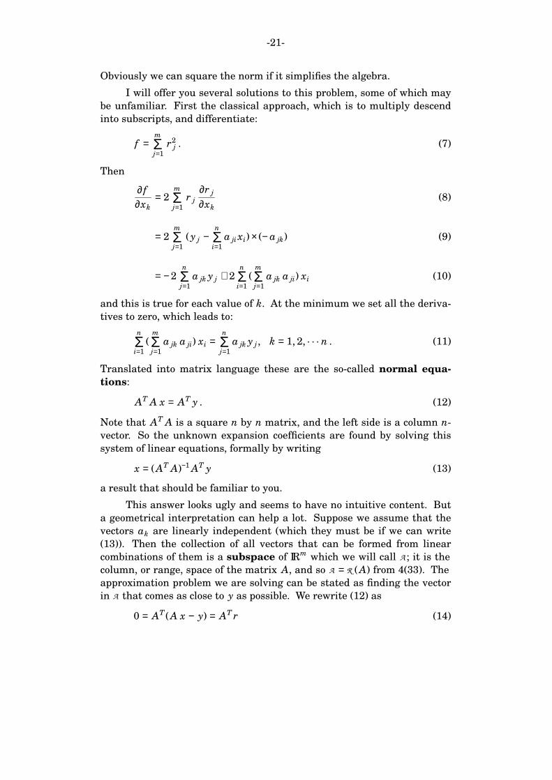
constraint, that must hold for all solutions. The Figure 6.1, taken from
GIT, show the general idea for single condition. If the constraint condi-
tion is expressed the in form:
g(x) = 0 (1)
then the minimum of the constrained problem
x ∈ IRmmin f (x) with g(x) = 0 (2)
occurs at a stationary point of the unconstrained function function
u(x, µ) = f (x) − µ g(x) (3)
where we must consider variations of x and µ; of course µ is called a
Lagrange multiplier. If there are n constraint conditions in the from
gk(x) = 0, k = 1, 2, . . . n, each would be associated with its own Lagrange
multiplier:
u(x, µ1, µ2, . . . µn) = f (x) −n
k=1Σ µk gk(x) . (4)
Figure 6.1: An optimization problem in 2 unknowns with 1 con-
straint.

-27-
As an example consider again the overdetermined LS problem
solved by 5(13). We wish to find the minimum of the function
f (r) = ||r||2, with r ∈ IRm. As an unconstrained problem the answer is
obviously zero. But we have the following m conditions on r:
0 = y − Ax + r (5)
where y ∈ IRm and A ∈ IRm × n are known, while the vector x ∈ IRn is also
unknown and free to vary. So, writing (5) out in components and giving
each row its own Lagrange multiplier, (4) becomes for this problem
u(r, x, µ l) =m
j=1Σ r2
j −m
j=1Σ µ j(y j −
n
k=1Σ a jk xk + r j) . (6)
Differentiating over ri, xi and µ i, the stationary points of u occur when
∂u
∂ri
= 0 = 2ri − µ i (7)
∂u
∂xi
= 0 = −m
j=1Σ a ji µ j (8)
∂u
∂µ i
= 0 = yi −n
k=1Σ aik xk + ri . (9)
Equation (7) says the vector of Lagrange multipliers µ = 2r; then using
this fact and translating (8), (9) into matrix notation:
AT µ = 2AT r = 0 (10)
Ax − r = y . (11)
If we multiply (11) from the left with AT and use (10) we get the normal
equations 5(12) again. But let us do something else: we combine (10) and
(11) into a single linear system in which the unknown consists of both x
and r:
Figure 6.2: An example of loss of sparseness in forming the normal
equations.

-28-
−Im
AT
A
On
r
x
=
y
0
(12)
where Im ∈ IRm×m is the unit matrix, where On ∈ IRn × n is square matrix
of all zeros. This system has the same content as the normal equations,
but solves for the residual and the coefficients at the same time. If A is
sparse, (12) can be a better way to solve the LS problem than by the nor-
mal equations or by QR, particularly as QR does not have a good adapta-
tion to sparse systems. The situation is illustrated for a common form of
overdetermined problem in Figure 6.2.
We turn next to the so-called underdetermined least-squares
problem. While the overdetermined LS problem occurs with monotonous
regularity in statistical parameter estimation problems, the underdeter-
mined LS problem looks quite a lot like an inverse problem. Instead of
trying to approximate the known y by a vector in the column space of A,
we can match it exactly: we have
y = Ax . (13)
where A ∈ IRm × n, but now m < n and A is of full rank. This is a finite-
dimensional version of the linear forward problem, in which the number
of measurements, y, is less than the number of parameters in the model
x. So instead of looking for the smallest error in (13), which is now zero,
we ask instead for the smallest model, x. We are performing a simplified
regularization, in which size, here represented by the Euclidean length,
stands for simplicity. This problem is solved just as the last one, with a
collection of m Lagrange multipliers to supply the constraints given by
(13), but with ||x||2
being minimized instead of ||r||2. I’ll run through
the process quickly. The unconstrained function is
u(x, µk) =n
j=1Σ x2
j −m
i=1Σ µ i(
n
k=1Σ aik xk − yi) (14)
∂u
∂x j
= 2x j −m
i=1Σ aij µ i (15)
∂u
∂µ i
= −n
k=1Σ aik + yi . (16)
Setting these derivatives to zero leads to a pair of linear systems which
can be written in matrix notation
x = ½AT µ (17)
Ax = y (18)
Equation (17) contains a key piece of information: the norm minimizer
lies in the range space of A or, in other words, x is a linear combination of
the column vectors of A. If we substitute the first of these into the second
-29-
we have
½AAT µ = y . (19)
which we imagine solving somehow, then substituting for µ in the first
member of (17)
x = AT (AAT )−1 y . (20)
These are the normal equations for the underdetermined (smallest norm)
problem. Explicitly following equation (20) is rarely a good way to com-
pute the solution, however. First, if matrix A is sparse we loose that
property forming AAT : then it is better to combine (17) and (18) into a
large sparse system combining µ and x in a longer unknown vector as we
did in (12). Second, we can use QR to find a numerically stable result.
Like the normal equations, (19) too suffers from poor conditioning
numerically. And as before QR comes to the rescue, but in a cute way.
Recall that the classic QR factorization works only if m ≥ n, here that is
violated. So we write instead that
AT = QR or A = RT QT . (21)
Then (13) can be written
y = RT QT x = RT x (22)
where x ∈ IRm is just QT x. Then, since Q is an orthogonal matrix
x = Qx (23)
and it follows that x and x have the same norm, ie. Euclidean length.
Recall that R is upper triangular; so (22) is
y = [RT1 O]
x1
x2
(24)
where R1 ∈ IRn × n, and x1 ∈ IRn. If we multiply out the partitioned matrix
we see that
y = RT1 x1 + O x2 = RT
1 x1 . (25)
Because the second term vanishes, (25) shows that we can choose x2 (the
bottom part of x) in any way we like and it will not affect the match to
the data: only x1 influences that. So we match the data exactly by solving
the system
RT1 x1 = y . (26)
Now observe that
||x||2 = || x||
2 = || x1||2 + || x2||
2. (27)
So to match the data we solve (26), then to get the smallest norm we sim-
ply put x2 = 0. Thus x has been found that minimizes the norm, and the
corresponding x is recovered from (23).
-30-
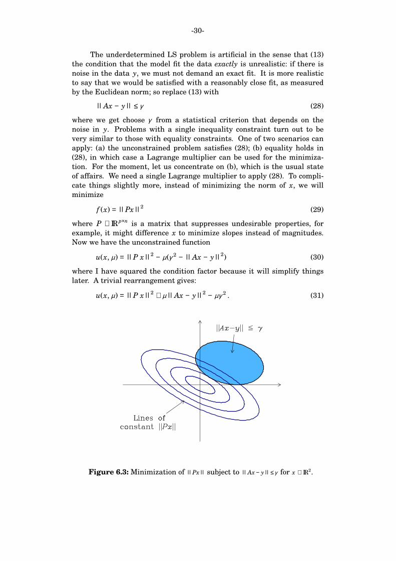
The underdetermined LS problem is artificial in the sense that (13)
the condition that the model fit the data exactly is unrealistic: if there is
noise in the data y, we must not demand an exact fit. It is more realistic
to say that we would be satisfied with a reasonably close fit, as measured
by the Euclidean norm; so replace (13) with
||Ax − y|| ≤ γ (28)
where we get choose γ from a statistical criterion that depends on the
noise in y. Problems with a single inequality constraint turn out to be
very similar to those with equality constraints. One of two scenarios can
apply: (a) the unconstrained problem satisfies (28); (b) equality holds in
(28), in which case a Lagrange multiplier can be used for the minimiza-
tion. For the moment, let us concentrate on (b), which is the usual state
of affairs. We need a single Lagrange multiplier to apply (28). To compli-
cate things slightly more, instead of minimizing the norm of x, we will
minimize
f (x) = ||Px||2
(29)
where P ∈ IRp×n is a matrix that suppresses undesirable properties, for
example, it might difference x to minimize slopes instead of magnitudes.
Now we have the unconstrained function
u(x, µ) = ||P x||2 − µ(γ 2 − ||Ax − y||
2) (30)
where I have squared the condition factor because it will simplify things
later. A trivial rearrangement gives:
u(x, µ) = ||P x||2 + µ||Ax − y||
2 − µγ 2 . (31)
Figure 6.3: Minimization of ||Px|| subject to ||Ax − y|| ≤γ for x ∈ IR2.
-31-
It can be shown (see GIT, Chapter 3) that µ > 0. Then for a fixed value of
µ, the function u can be interpreted as finding a compromise between two
undesirable properties, large P x, and large data misfit. If we minimize
over x with a small µ we give less emphasis to misfit and find models that
keep P x very small; and conversely, large µ causes minimization of u to
yield x with small misfit. This is an example of a trade-off between two
incompatible quantities: it is shown in GIT that decreasing the misfit
always increases the penalty norm, and vice versa.
We could solve this problem by differentiating in the usual tedious
wa y. Instead we will be a bit more clever. As usual, differentiating by µjust gives the constraint (28). The derivatives on x don’t see the γ term in
(31) so we can drop that term when we consider the stationary points of u
with respect to variations in x:
u(x) = ||P x||2 + µ||Ax − y||
2(32)
= ||Px − 0||2 + ||µ½ Ax − µ½ y||
2. (33)
Both of the terms are norms acting on a vector; we can make the sum into
a single squared norm of a longer vector, the reverse of what we did on
equation 5(24):
u(x) =
P
µ½ A
x −
0
µ½ y
2
(34)
= ||Cx − d||2
. (35)
The matrix C ∈ IR( p+m)×n must be tall, that is p + m > n, or the original
problem has a trivial solution (Why?), (35) is just an ordinary overdeter-
mined least squares problem; indeed the matrix C is the one illustrated in
Figure 6.2. So for any given value of µ, we can find the corresponding x
through our standard LS solution. But this doesn’t take care of (28). The
only way to satisfy this misfit criterion is by solving a series of versions of
(35) for different guesses of µ in an iterative way, because unlike all the
other systems we have met so far, this equation is nonlinear. We will dis-
cuss the details later (see GIT, Chap 3).
What about scenario (a)? We need to verify that the unconstrained
problem, the minimizer of ||Px||2
satisfies (28). When P is nonsingular,
that is easy, because then the unique solution is x = 0, and that can be
checked trivially in (28). If P is singular the solution to the unconstrained
problem is not unique, and we could set up the minimization of ||Ax − y||
over the null space of P. But in fact we will discover in solving (31) that
(28) is satisfied for all µ > 0 as part of the search in µ, so solving (28) with
an equality is all we need ever to do.
-32-
7. Other Matrix Factorizations
The QR factorization is one of a number of matrix factorizations that
appear in the numerical analysis of linear algebra. The rule that numeri-
cal analysts repeat with great regularity is that to solve the linear system
Ax = y (1)
never, never, never calculate the inverse A−1 and multiply this into the vec-
tor y. The reasons are that it is numerically inaccurate, and inefficient.
The recommended way is via one of several factorizations. To solve (1) in
MATLAB you should always type:
x = A \ y ;Recall that when A ∈ IRm × n and the problem is overdetermined ( m > n),
this gets you the least-squares solution via QR. When m = n, the system
is solved, with QR, but by Gaussian elimination which can also be writ-
ten as a matrix factorization called LU decomposition:
A = LU . (2)
Here A, L,U ∈ IRn × n and L is lower triangular, while U is upper triangu-
lar, called U because for some unknown reason the word ‘upper’ is always
used here instead of ‘right’ (which is always the name used in QR). For-
mally the solution to (1), once you have the LU factors is to solve by back
substitute the two systems
Lz = y, and Ux = z . (3)
You don’t need to know this of course just to use back-slash. Unlike QR
factorization, LU decomposition of a sparse matrix A results in two
sparse factors L and U , which is a very important property for large sys-
tems of equations.
A special case arises when A is symmetric, and positive definite.
Then A can be factored with the Cholesky factorization
A = L LT (4)
where L is lower triangular. Notice that this factorization is almost like a
square root of A, and is handy in a number of situation when a matrix
square root could be useful. Cholesky factorization is one of the fastest
and must numerically stable schemes in numerical linear algebra.
Next let me briefly remind you about the elementary theory of eigen-
value systems for square matrices. You will recall that a square symmet-
ric matrix always has eigenvalues, which are the real numbers λ satisfy-
ing
Au = λ u, and u ≠ 0 . (5)
When A ∈ IRn × n is not symmetric λ need not be real, and in some cases
there are no solutions to (5); the symmetric case covers almost all those of
practical interest. When A is symmetric, there are at most n distinct val-
ues of λ , call them λ k, and n corresponding eigenvectors uk.
-33-
Conventionally, these are normalized so that ||uk|| = 1, in the 2-norm. A
most important property of the eigenvectors is that they are mutually
orthogonal:
uTj uk = 0, when j ≠ k . (6)
When there are fewer than n eigenvalues, the system is said to be degen-
erate and can be treated as if there are repeated values of λ ; and then the
eigenvectors of the degenerate eigenvalues are not uniquely defined. But
they can always be chosen to be orthogonal so that (6) can be forced to be
true, and always is in computer programs. The simplest illustration of all
this is the unit matrix: every vector is an eigenvector of I with eigenvalue
1; so the eigensystem is n-fold degenerate, that is, there are n eigenval-
ues, all the same, all equal to one.
The eigenvalue problem can be written as a matrix factorization, as
we shall now see. Form the square matrix U from columns of the orthogo-
nal eigenvectors:
U = [u1, u2, . . . un] (7)
The matrix U is an orthogonal matrix, because its columns are mutually
orthogonal unit vectors. Then
AU = [Au1, Au2, . . . Aun] = [λ 1u1, λ 2u2, . . . λ nun] = UΛ (8)
where Λ = diag (λ 1, λ 2, . . . λ n). Now multiply on the right with UT and we
have the spectral factorization of A:
A = UΛUT (9)
This can be written another way that is most instructive:
A = λ 1u1uT1 + λ 2u2uT
2 + . . . λ nunuTn (10)
= λ 1 P1 + λ 2 P2 + . . . λ n Pn (11)
Here the outer product matrices ukuTk are projection matrices each of
which maps a vector into the subspace comprised of the corresponding
eigenvector. Equation (11) is decomposing the action of A into compo-
nents in an orthogonal coordinate system, where each component receives
a particular magnification by the corresponding λ k. Think about what
this means when there is degeneracy. It should be observed that numeri-
cal techniques for discovering the eigenvalues and eigenvectors of sym-
metric matrices are based on performing the factorization (9), not on eval-
uating some huge determinant, which would take an eternity.
There is a spectral factorization for nonsquare matrices as well,
called singular value decomposition usually called SVD. Suppose
A ∈ IRm × n with m > n, then A can be factorized into the product of three
matrices, two orthogonal and one diagonal:
A = U Σ V T (12)

-34-
where U ∈ IRm×m and V ∈ IRn × n are orthogonal and Σ ∈ IRm × n with
Σ = diag (s1, s2, . . . sn) (13)
The real numbers sk ≥ 0 are called the singular values of A. One can
solve LS problems with SVD. There are number of people who claim SVD
is the answer to almost all LS problems because of its great numerical
stability and because of its use in censoring the poorly resolved features
in simple minimization problems. I believe these advantages are usually
overstated; also the procedure is numerically very expensive, and not
readily adapted to sparse systems, and therefore not suitable for large
systems.
-35-
SIO 230 Geophysical Inverse Theory 2009
Supplementary Notes
8. A New Magnetic Problem
In GIT the first few chapters revolve around a marine magnetic problem
based on a small set of artificial ‘‘data’’, supposedly collected at the North
Pole. This example is too simple these days for two reasons: first, the
number of observations (thirty) is trivially small; second, the idealization
of the problem covers up so many of the real difficulties, particularly the
questions surrounding the proper form of the forward problem. I want to
work with a more realistic illustration, based on actual data, to give you a
better idea of how to handle real-life situations that you may come across.
However, I still want to stick to a one-dimensional geometry, to keep the
graphics simple. It is another marine magnetic problem, like the one in
GIT, except that the observations were taken near the sea floor in 1995 on
a deep-tow vehicle (the ‘‘fish’’) built by the Marine Physical Lab at SIO.
The profile runs across the Juan de Fuca rise (35°N, 130°W) off the coast
of Washington, with a strike direction of 107° east of true north; these
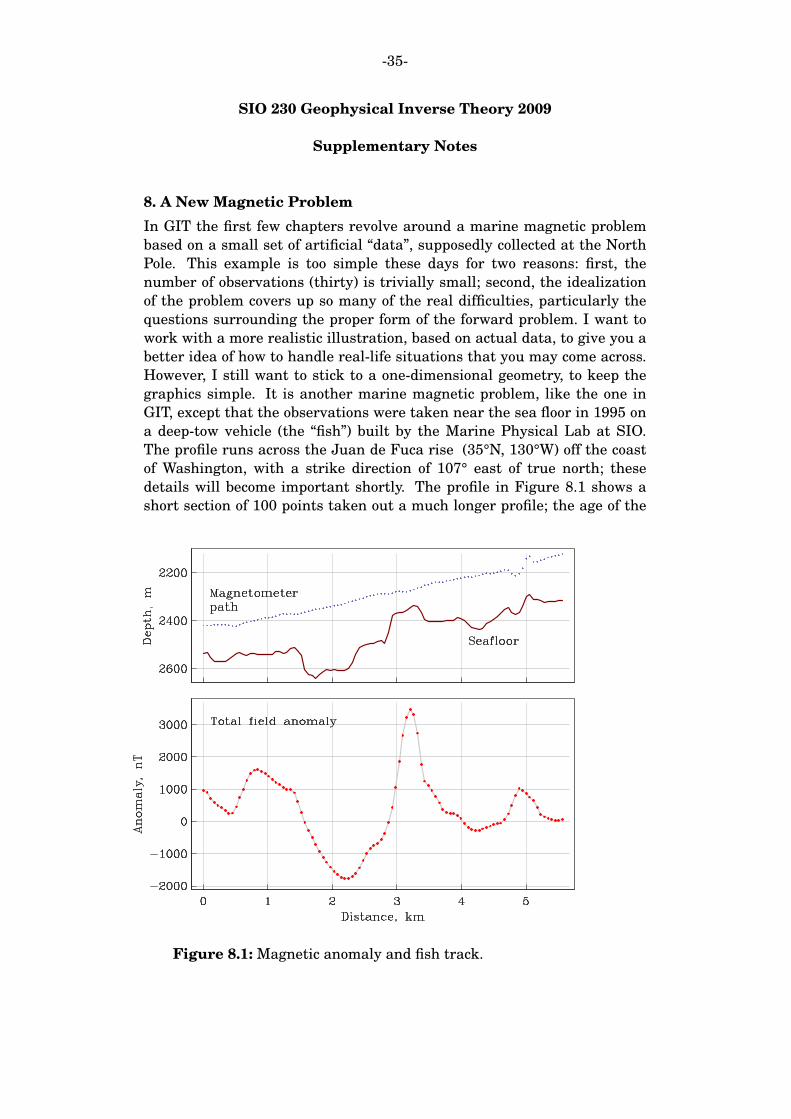
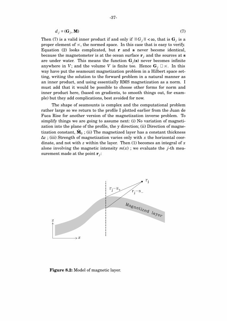
details will become important shortly. The profile in Figure 8.1 shows a
short section of 100 points taken out a much longer profile; the age of the
Figure 8.1: Magnetic anomaly and fish track.
-36-
oceanic crust is about 0.2 Ma, so we are in the Bruhnes normal chron,
which ended 0.78 Ma ago.
In a moment we are going to make a number of simplifications to get
at the crustal magnetization here. Recall from 2(1-2) that the original
magnetization forward problem has a solution that looks like this:
∆B(r) =V
∫ G(s, r) ⋅ M(s) d3s (1)
with G fully expanded now to
G(s, r) =µ0
4πB0 ⋅ ∇ ∇
1
R=
µ0
4π
3B0 ⋅ (r −s)(r −s)
R5−
B0
R3
(2)
and R = |r −s|. Remember the magnetization M is a vector-valued func-
tion of position s within the volume V ; the grad acts on the s coordinate
here, although since G(r, s) = G(s, r) that is unimportant in (2). In (1) G is
known and M is the function we seek. In fact we do not have continuous
values of ∆B, but samples at specific points on the sea surface
r1, r2, . . . rm. So we can specialize (1) to this situation
d j = ∆B(r j) =V
∫ G j(s) ⋅ M(s) d3s, j = 1, 2, . . . m (3)
where we assign particular function G j(s) to each observation:
G j(s) = G(s, r j) =µ0
4πB0 ⋅ ∇ ∇
1
|r j − s|(4)
Notice that each measured number d j is obtained in (3) via a linear
functional of the unknown M. The set of vector-valued magnetizations
within the volume V can be considered to be linear vector space V ; there
are obvious rules for adding two magnetizations and for multiplying a
given magnetization by a scalar. Suppose we equip V with the following
inner product:
(f, g) =V
∫ f(s) ⋅ g(s) d3s (5)
The we automatically get a norm for the space; the new normed space
will be called H for Hilbert. The implied size of a given magnetization
function is this:
||M|| =√ V
∫ M ⋅ M d3s (6)
This is almost the RMS magnetization; to get ||M|| to be RMS magneti-
zation we have to normalize by the volume: MRMS = ||M||/V ½.
The key question is whether or not we can write (3) as an inner
product or not. It is a linear functional as we already stated, but is it a
bounded linear functional? Suppose I write (3) as an inner product:
-37-
d j = (G j , M) (7)
Then (7) is a valid inner product if and only if ||G j|| < ∞, that is G j is a
proper element of H , the normed space. In this case that is easy to verify.
Equation (2) looks complicated, but r and s never become identical,
because the magnetometer is at the ocean surface r j and the sources at s
are under water. This means the function G j(s) never becomes infinite
anywhere in V ; and the volume V is finite too. Hence G j ∈ H . In this
wa y have put the seamount magnetization problem in a Hilbert space set-
ting, writing the solution to the forward problem in a natural manner as
an inner product, and using essentially RMS magnetization as a norm. I
must add that it would be possible to choose other forms for norm and
inner product here, (based on gradients, to smooth things out, for exam-
ple) but they add complications, best avoided for now.
The shape of seamounts is complex and the computational problem
rather large so we return to the profile I plotted earlier from the Juan de
Fuca Rise for another version of the magnetization inverse problem. To
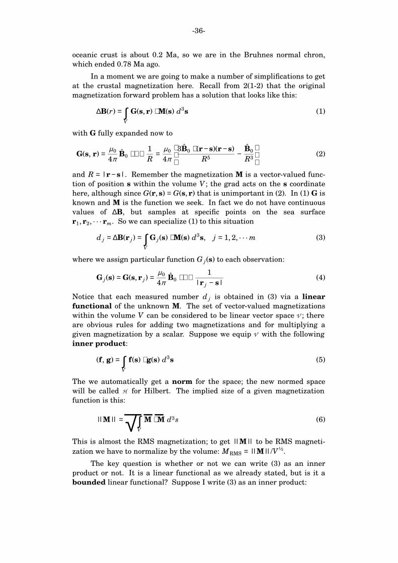
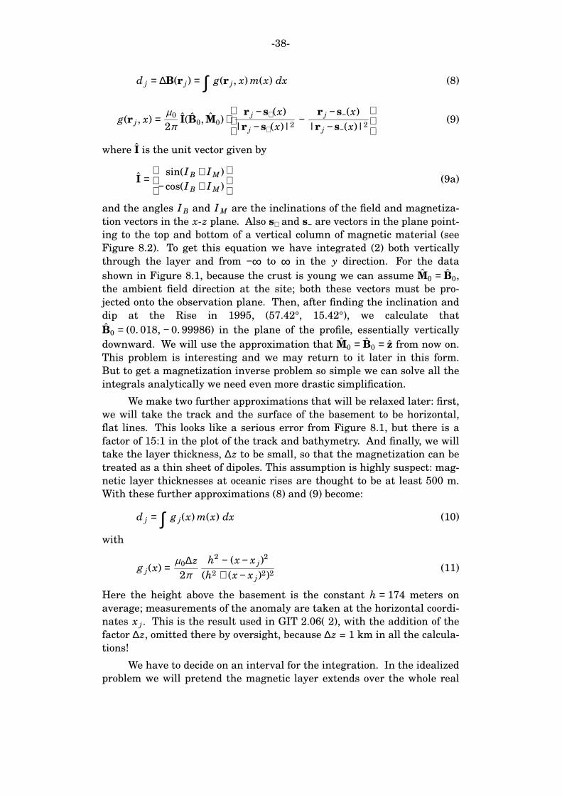
simplify things we are going to assume next: (i) No variation of magneti-
zation into the plane of the profile, the y direction; (ii) Direction of magne-
tization constant, M0 ; (ii) The magnetized layer has a constant thickness
∆z ; (iii) Strength of magnetization varies only with x the horizontal coor-
dinate, and not with z within the layer. Then (1) becomes an integral of x
alone involving the magnetic intensity m(x) ; we evaluate the j-th mea-
surement made at the point r j :
Figure 8.2: Model of magnetic layer.
-38-
d j = ∆B(r j) = ∫ g(r j , x) m(x) dx (8)
g(r j , x) =µ0
2πI(B0, M0) ⋅
r j −s+(x)
|r j −s+(x)|2−
r j −s−(x)
|r j −s−(x)|2
(9)
where I is the unit vector given by
I =
sin(I B + I M )
− cos(I B + I M )
(9a)
and the angles I B and I M are the inclinations of the field and magnetiza-
tion vectors in the x-z plane. Also s+ and s− are vectors in the plane point-
ing to the top and bottom of a vertical column of magnetic material (see
Figure 8.2). To get this equation we have integrated (2) both vertically
through the layer and from −∞ to ∞ in the y direction. For the data
shown in Figure 8.1, because the crust is young we can assume M0 = B0,
the ambient field direction at the site; both these vectors must be pro-
jected onto the observation plane. Then, after finding the inclination and
dip at the Rise in 1995, (57.42°, 15.42°), we calculate that
B0 = (0. 018, − 0. 99986) in the plane of the profile, essentially vertically
downward. We will use the approximation that M0 = B0 = z from now on.
This problem is interesting and we may return to it later in this form.
But to get a magnetization inverse problem so simple we can solve all the
integrals analytically we need even more drastic simplification.
We make two further approximations that will be relaxed later: first,
we will take the track and the surface of the basement to be horizontal,
flat lines. This looks like a serious error from Figure 8.1, but there is a
factor of 15:1 in the plot of the track and bathymetry. And finally, we will
take the layer thickness, ∆z to be small, so that the magnetization can be
treated as a thin sheet of dipoles. This assumption is highly suspect: mag-
netic layer thicknesses at oceanic rises are thought to be at least 500 m.
With these further approximations (8) and (9) become:
d j = ∫ g j(x) m(x) dx (10)
with
g j(x) =µ0∆z
2πh2 − (x − x j)
2
(h2 + (x − x j)2)2
(11)
Here the height above the basement is the constant h = 174 meters on
average; measurements of the anomaly are taken at the horizontal coordi-
nates x j . This is the result used in GIT 2.06( 2), with the addition of the
factor ∆z, omitted there by oversight, because ∆z = 1 km in all the calcula-
tions!
We have to decide on an interval for the integration. In the idealized
problem we will pretend the magnetic layer extends over the whole real
-39-
line. This gross idealization does not get us into trouble until a bit later,
and is very handy for solving the integrals. If we like the norm
||m|| =
∞
−∞∫ m(x)2 dx
½
(12)
then the space of magnetization models becomes the classic Hilbert space
L2(−∞, ∞), with inner product
( f , g) =∞
−∞∫ f (x) g(x) dx (13)
Is (11) an inner product in this space? The answer is yes if we can show
that
||g j||2 =
µ20∆z2
4π2
∞
−∞∫
(h2 − (x − x j)2)2
(h2 + (x − x j)2)4
dz (14)
is finite. Later we will evaluate this messy integral exactly. For now we
can show it is bounded, by a couple of simple observations: the function
g j(x)2 is bounded and continuous (in fact it is analytic on the real line); as
|x| →∞ we can easily verify that g(x) → µ0∆z/2πx2 so that g(x)2 → con-
stant /x4. This dies awa y fast enough to have a finite integral and there
we can write (10) as
d j = (g j , m), j = 1, 2, . . . m (15)
Again, this may not be the only norm we will want to use, but to get
things started L2(−∞, ∞) is a good place to start.
You may be asking, when would the linear functions fail to be
bounded, and what would be the consequences of that failure? In this
problem, we can cause the integrals like (14) to be undefined simply by
setting h the height of the observation line, go to zero, effectively setting
the magnetometer directly on the sources, instead of above them; this is
not an impossible experimental geometry. One way to look at the failure
is to examine the limit as h tends to zero: we find the norm minimizing
magnetization becomes more and more closely concentrated around the
observation sites, and has a smaller and smaller norm, in the limit,
||m|| = 0. The model space L2 is inappropriate because it does not lead
to a geophysically plausible, let alone a simple solution. The original jus-
tification for norm minimizers was that they should select models with
the fewest extraneous features, to be as bland and unobjectionable as pos-
sible. When h is set to zero, L2 fails to do this, and we should look for a
different approach; the best way is to leave Hilbert space entirely.
-40-
9. The Continuous Problem
Before getting into the application of our general Hilbert-space based
approach, let us look at a naive treatment of the 1-D, flat layer problem
that relies on its special characteristics. While the method in its bare
form fails miserably, it provides some useful insights of a general nature
and, as we shall see later, it can be modified to yield quite satisfactory
answers. First pretend that we have dense observations on the whole real
line. Then 8(10) becomes
d(y) =∞
−∞∫ k(y − x) m(x) dx (1)
where
k(x) =µ0∆z
2πh2 − x2
(h2 + x2)2(2)
Written this way, it is clear that the solution to the forward problem when
the data d are known on (−∞, ∞) is a convolution.
Convolutions are very common in geophysics, and just as in this
case, we frequently want to undo them: this is called the deconvolution
problem. Geophysical examples include undoing the effects of an instru-
ment, like a seismometer, or a magnetometer (Constable and Parker,
1991), or removing path effects from a seismogram using the empirical
Green’s function (Prieto, et al, 2006).
Whenever you see a convolution (which you know can be written
d = k ∗ m) you should think of the Convolution Theorem, which says
F [k ∗ m] =F [k] F [m] = k m (3)
where of course F is the Fourier transform (FT) given by
F [ f ] = f (λ ) =∞
−∞∫ f (x) e−2πiλ x dx (4)
Thus, if we take the FT of (1) we see
d = k m (5)
and the solution to the inverse problem is obtained merely by division,
since the complicated integral in (1) has been converted into a simple mul-
tiplication. (Mathematicians would say the convolution has been diago-
nalized.) The result for m is just
m(x) =F −1
d
k
(6)
The inverse problem is apparently finished, since the solution has been
reduced to three FTs and a division.
In fact we can go one step further: the FT of k(x) can be found in
terms of elementary functions. Those of you who took SIO-239 from me

-41-
should think about how to go about this calculation, starting from the
well-known FT of 1/(h2 + x2). I will just give you the answer, the amaz-
ingly simple:
k(λ ) = π µ0∆z |λ | e−2πh|λ | (7)
This function is shown in Figure 9.1; it is obviously even in λ .
At first glance, equation (6) seems to imply there is a unique solution
to the inverse problem: for every function d, there is a unique d and so
there is just one m and one m that results: in other words, complete and
exact data provide a single, one-dimensional magnetization model m(x).
That is in complete contrast to the 3-D problem considered at the begin-
ning of the class, where exact data can be matched with a enormous array
of different internal magnetizations. However, things aren’t quite so
straightforward. Look at (7): notice that k(0) = 0. This means that the
integral of k(x) over all x vanishes, and therefore any constant magnetiza-
tion generates zero magnetic anomaly. A constant magnetization may be
present in any amount and it will always be undetectable: it is the mag-
netic annihilator for the problem. Hence the solution to this inverse
problem is not unique — there is a single uncontrolled degree of freedom.
We conclude that the many additional assumptions and simplifications we
introduced have almost, but not quite, suppressed the vast ambiguity of
the original problem posed in Section 2 of these notes.
The analytic solution also highlights the instability associated with
short-wavelength anomalies. Equation (6) states that to obtain the mag-
netization function we must apply a spatial filter with transfer function
k(λ )−1, a function shown in Figure 9.1. Because k(λ ) decays essentially
exponentially, small-scale components of d are magnified with an expo-
nentially growing factor as the scale decreases. With realistic signals,
noise does not decay exponentially with wavenumber, and so above some
value of λ , noise will be preferentially amplified by this deconvolution.
Figure 9.1: The function k(λ ) and its reciprocal. The constant
γ = π µ0∆z/h.
-42-
And the same thing happens, though less explosively at small wavenum-
bers. So both the longest and the short wavelengths are amplified in a
singular way, making them the least reliable parts of the solution.
Applying (6), an ‘‘exact’’ solution, to real data presents serious diffi-
culties. We don’t have a continuous function d(x) for all real x, but finite
set of numbers. If we interpolate the samples to create values at short
scales, we are introducing values just where the filter 1/k generates the
greatest exaggeration. If we extend the finite profile by some other kind
of extrapolation, the longest wavelengths are invented, and yet these are
given the unbounded emphasis by the filter! So, while we could attempt
to approximate the analytic inversion with a Fast Fourier Transform of
the actual data, we will turn instead to a process that takes into account
the finiteness of the data set, and its uncertainties.
References
Constable, C. G. and Parker, R. L., Deconvolution of long-core paleomag-
netic measurements: Spline therapy for the linear problem, Geophys. J.
Int. 104, 453-468, 1991.
Prieto, G. A., Parker, R. L., Vernon, F. L., Shearer, P., M., and Thomson, D.
J., Uncertainties in earthquake source spectrum estimation using empiri-
cal Green functions, in Earthquakes: Radiated Energy and the Physics of
Faulting, Geophysical monograph 170, eds Abercrombie, McGarr,
Kanamori, and Di Toro, American Geophysical Union, Washington, 2006.
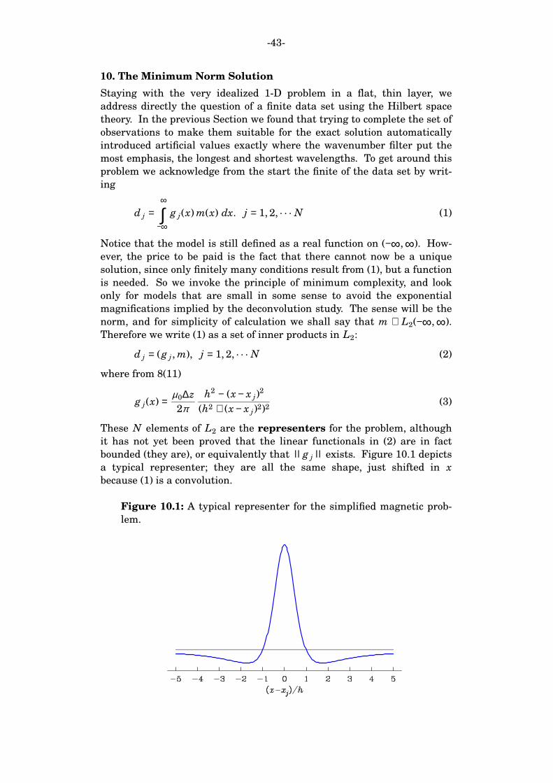
-43-
10. The Minimum Norm Solution
Staying with the very idealized 1-D problem in a flat, thin layer, we
address directly the question of a finite data set using the Hilbert space
theory. In the previous Section we found that trying to complete the set of
observations to make them suitable for the exact solution automatically
introduced artificial values exactly where the wavenumber filter put the
most emphasis, the longest and shortest wavelengths. To get around this
problem we acknowledge from the start the finite of the data set by writ-
ing
d j =∞
−∞∫ g j(x) m(x) dx. j = 1, 2, . . . N (1)
Notice that the model is still defined as a real function on (−∞, ∞). How-
ever, the price to be paid is the fact that there cannot now be a unique
solution, since only finitely many conditions result from (1), but a function
is needed. So we invoke the principle of minimum complexity, and look
only for models that are small in some sense to avoid the exponential
magnifications implied by the deconvolution study. The sense will be the
norm, and for simplicity of calculation we shall say that m ∈ L2(−∞, ∞).
Therefore we write (1) as a set of inner products in L2:
d j = (g j , m), j = 1, 2, . . . N (2)
where from 8(11)
g j(x) =µ0∆z
2πh2 − (x − x j)
2
(h2 + (x − x j)2)2
(3)
These N elements of L2 are the representers for the problem, although
it has not yet been proved that the linear functionals in (2) are in fact
bounded (they are), or equivalently that ||g j|| exists. Figure 10.1 depicts
a typical representer; they are all the same shape, just shifted in x
because (1) is a convolution.
Figure 10.1: A typical representer for the simplified magnetic prob-
lem.
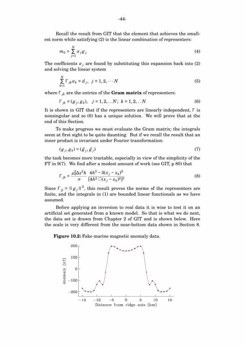
-44-
Recall the result from GIT that the element that achieves the small-
est norm while satisfying (2) is the linear combination of representers:
m0 =N
j=1Σ α j g j (4)
The coefficients α j are found by substituting this expansion back into (2)
and solving the linear system
N
k=1Σ Γ jkα k = d j , j = 1, 2, . . . N (5)
where Γ jk are the entries of the Gram matrix of representers:
Γ jk = (g j , gk), j = 1, 2, . . N ; k = 1, 2, . . N (6)
It is shown in GIT that if the representers are linearly independent, Γ is
nonsingular and so (6) has a unique solution. We will prove that at the
end of this Section.
To make progress we must evaluate the Gram matrix; the integrals
seem at first sight to be quite daunting. But if we recall the result that an
inner product is invariant under Fourier transformation:
(g j , gk) = ( g j , g j) (7)
the task becomes more tractable, especially in view of the simplicity of the
FT in 9(7). We find after a modest amount of work (see GIT, p 80) that
Γ jk =µ2
0∆z2h
π4h2 − 3(x j − xk)2
[4h2 + (x j − xk)2]3(8)
Since Γ jj = ||g j||2, this result proves the norms of the representers are
finite, and the integrals in (1) are bounded linear functionals as we have
assumed.
Before applying an inversion to real data it is wise to test it on an
artificial set generated from a known model. So that is what we do next,
the data set is drawn from Chapter 2 of GIT and is shown below. Here
the scale is very different from the near-bottom data shown in Section 8.
Figure 10.2: Fake marine magnetic anomaly data.
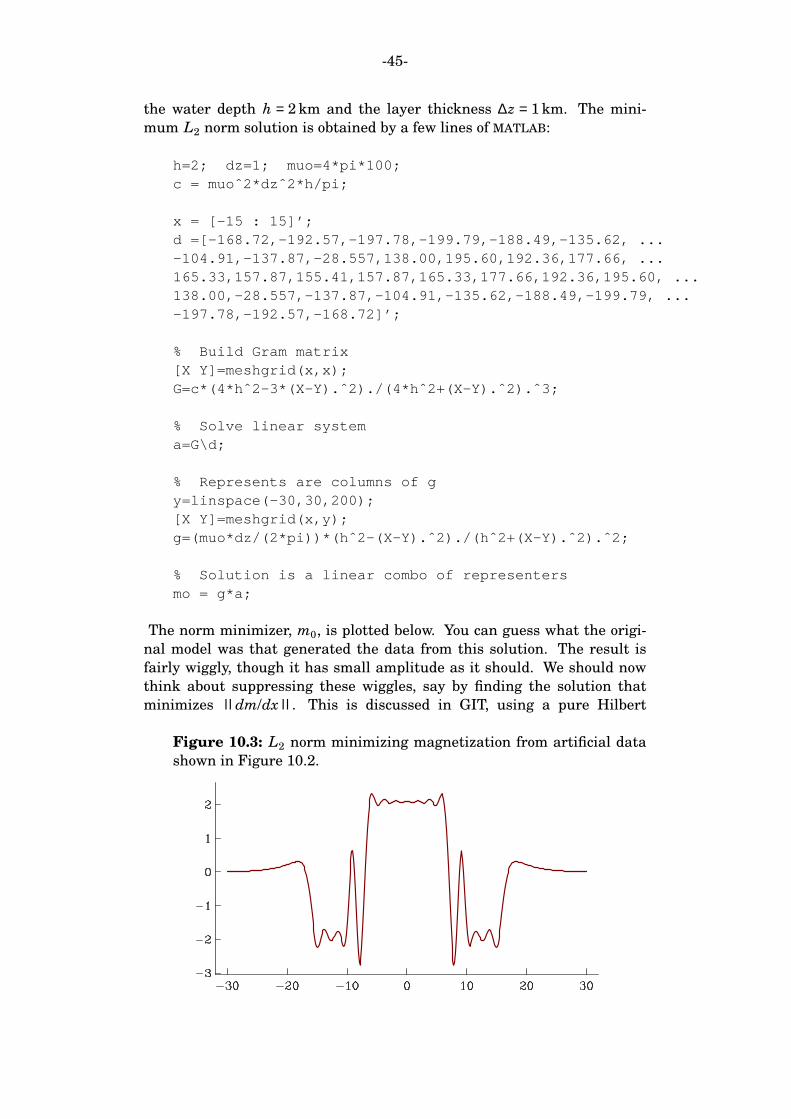
-45-
the water depth h = 2 km and the layer thickness ∆z = 1 km. The mini-
mum L2 norm solution is obtained by a few lines of MATLAB:
h=2; dz=1; muo=4*pi*100;c = muoˆ2*dzˆ2*h/pi;
x = [ -15 : 15]’;d =[-168.72,-192.57,-197.78,-199.79,-188.49,-135.62, ...-104.91,-137.87,-28.557,138.00,195.60,192.36,177.66, ...165.33,157.87,155.41,157.87,165.33,177.66,192.36,195.60, ...138.00,-28.557,-137.87,-104.91,-135.62,-188.49,-199.79, ...-197.78,-192.57,-168.72]’;
% Build Gram matrix[X Y]=meshgrid(x,x);G=c*(4*hˆ2-3*(X-Y).ˆ2)./(4*hˆ2+(X-Y).ˆ2).ˆ3;
% Solve linear systema=G\d;
% Represents are columns of gy=linspace(-30,30,200);[X Y]=meshgrid(x,y);g=(muo*dz/(2*pi))*(hˆ2-(X-Y).ˆ2)./(hˆ2+(X-Y).ˆ2).ˆ2;
% Solution is a linear combo of representersmo = g*a;
The norm minimizer, m0, is plotted below. You can guess what the origi-
nal model was that generated the data from this solution. The result is
fairly wiggly, though it has small amplitude as it should. We should now
think about suppressing these wiggles, say by finding the solution that
minimizes ||dm/dx||. This is discussed in GIT, using a pure Hilbert
Figure 10.3: L2 norm minimizing magnetization from artificial data
shown in Figure 10.2.
-46-
space method. We will look at this from a numerical view point in a later
Section. The results are not very impressive — the wiggles are still there.
In GIT the linear independence of the representers for the 1-D mag-
netic anomaly inverse problem was proved using the Fourier transform. I
will present here an alternative proof, which is more useful because it
gives a method that I have found works for a number of linear inverse
problems, especially those arising out of potential theory like this one.
The approach is successful for problems in two and three dimensional
problems too.
Here we have a set of N functions on the real line given by:
g j(x) =h2 − (x − x j)
2
(h2 + (x − x j)2)2
, j = 1, 2, . . . N (9)
where all the x j are different (why?). I have dropped all the constant fac-
tors for obvious reasons. Although the setting of the original problem is
the space L2(−∞, ∞), we can use properties of g j that functions in L2
don’t all possess for our proof. The normal way to prove this kind of
proposition is by contradiction: we shall assume the set is linearly
dependent and then show that leads to a contradiction. The statement
for LI is that there are scalars β j not all zero, such that
N
j=1Σ β j g j(x) = 0, for all x . (10)
If this is true, we can choose one of the functions gk multiplied by a
nonzero coefficient, and move it onto the other size thus:
gk(x) =j ≠ kΣ (− β j /β k) g j(x) (11)
which says that the representer gk can be built from a linear combination
of the others.
To get a contradiction we need to focus on a value of x where gk(x)
goes to infinity. There is no such place on the real line, but never mind —
we can choose x to be complex if we wish! Looking at (9) we see that the
denominator vanishes whenever (x − x j)2 = −h2 or
x∗ = x j ± ih . (12)
These are the singularities of g j in the complex x plane. Suppose now I
consider the function gk(x) in (11) when x − xk = ih + ε where ε is a small
real quantity of our choosing; in other words, x is very near a singular
point of the function gk(x). From the definition of gk we see that
-47-
gk(x) =h2 − (ih + ε )2
(h2 + (ih + ε )2)2= −
2h2 +2ihε + ε 2
ε 2(2ih + ε )2(13)
=1
2ε 21 + O(ε )
. (14)
It is clear that by making ε small enough we can get the magnitude of
gk(x) as large as we wish. For the same x on the other side of (11) we look
at the denominators and we see a value that does not go to zero as ε gets
small:
(h2 + (x − x j)2)2 = ((xk − x j + ε )2 +2ih(xk − x j + ε ))2 (15)
= (xk − x j + ε )2(xk − x j + ε +2ih)2 . (16)
This number is not zero for small ε because x j ≠ xk and both of the xs are
real. The same thing is true for every j on the right of (11). This means
that as ε tends to zero, the left side of (11) grows and grows, while the
right side tends to some constant value. That is a contradiction, which
means that constants like β j do not exist.
Almost exactly this argument works for the representers in the more
complicated magnetic problems considered in Section 8 of the Supplemen-
tary Notes, while the Fourier treatment probably could not be made to
apply. Setting up an equation like (11) in which one side is constant,
while the other grows to infinity (or shrinks to zero) is a classic way to
show linear dependence of a set of functions. Doing this in the complex
plane is a very natural thing, because every analytic function has a singu-
larity in the complex plane, except the constant.
-48-
11. The Numerical Alternative
The functional analysis approach to the norm minimization problem in
Hilbert space shows how an exact theory can be worked out retaining the
essential asymmetry between data and model: data are finite in number,
but the model is a function that lives on an infinite-dimensional space.
But real-world situations in which the Gram matrix can be calculated
exactly, while not nonexistent, are in the minority. I mention for your edi-
fication two of my papers where exact Gram matrices are in fact found:
Shure, L., Parker, R. L., and G. E. Backus: Harmonic splines for geomag-
netic modeling, in Phys. Earth Planet. Inter., 28, 215-29, 1982 and Parker,
R. L.: Calibration of the pass-through magnetometer-I. Theory, in Geo-
phys. J. Internat., 142, 371-83, 2000. Numerical methods will in any case
appear at some point in every calculation and so we will now develop a
treatment based on linear algebra that is founded on a finite-dimensional
approximation for the forward problem.
The key is that the linear functional that captures the solution to
the forward problem, written in Chapter 2 of GIT as
(g j , m) = d j , j = 1, 2, . . . M (1)
can be written in an approximation as a finite sum
gTj m = d j , j = 1, 2, . . . M (2)
where g j , m ∈ IRN ; so now the model and representers are vectors of
dimension N . Of course (2) is more compactly written
Gm = d (3)
where G ∈ IRM×N and d ∈ IRM and the rows of the matrix G are the (row)
vectors gTj . At this point in the class when the models are simple, we
tend to think of M, the number of data, being a lot smaller than the N
the dimension of the model space, but when big data sets are involved
that isn’t always the case.
In the vast majority of practical cases the inner product in (1) is rep-
resenting an integral, as in the inner product of L2. To make the transi-
tion to (2) one must discretize the underlying continuous problem. The
most primitive way of doing this which, quite honestly I prefer, is to break
the model space up into boxes and replace the integral by a simple sum.
On the real line, for example, in the simple one-dimensional magnetiza-
tion problem, we could use uniform sampling, ∆x, and then
b
a∫ f (x) dx =
N
k=1Σ wk f (a + (k −1)∆x) + ε (4)
where ∆x = (b − a)/(N −1), wk are a set of weights, and ε is the error
approximation. The easiest, and in most circumstances least accurate for-
mula of this kind is the trapezoidal rule where one takes:
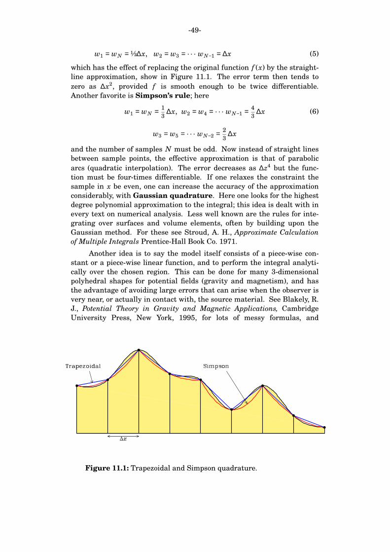
-49-
w1 = wN = ½∆x, w2 = w3 = . . . wN−1 = ∆x (5)
which has the effect of replacing the original function f (x) by the straight-
line approximation, show in Figure 11.1. The error term then tends to
zero as ∆x2, provided f is smooth enough to be twice differentiable.
Another favorite is Simpson’s rule; here
w1 = wN = 1
3∆x, w2 = w4 = . . . wN−1 = 4
3∆x (6)
w3 = w5 = . . . wN−2 = 2
3∆x
and the number of samples N must be odd. Now instead of straight lines
between sample points, the effective approximation is that of parabolic
arcs (quadratic interpolation). The error decreases as ∆z4 but the func-
tion must be four-times differentiable. If one relaxes the constraint the
sample in x be even, one can increase the accuracy of the approximation
considerably, with Gaussian quadrature. Here one looks for the highest
degree polynomial approximation to the integral; this idea is dealt with in
every text on numerical analysis. Less well known are the rules for inte-
grating over surfaces and volume elements, often by building upon the
Gaussian method. For these see Stroud, A. H., Approximate Calculation
of Multiple Integrals Prentice-Hall Book Co. 1971.
Another idea is to say the model itself consists of a piece-wise con-
stant or a piece-wise linear function, and to perform the integral analyti-
cally over the chosen region. This can be done for many 3-dimensional
polyhedral shapes for potential fields (gravity and magnetism), and has
the advantage of avoiding large errors that can arise when the observer is
very near, or actually in contact with, the source material. See Blakely, R.
J., Potential Theory in Gravity and Magnetic Applications, Cambridge
University Press, New York, 1995, for lots of messy formulas, and
Figure 11.1: Trapezoidal and Simpson quadrature.
-50-
FORTRAN code too! This approach may be necessary when the representer
is unbounded (as it is with gravity or magnetic measurements made on
the surface of the source region) because then trapezoidal or Simpson
quadrature can give infinite answers.
Let us try some of these ideas out on the 1-dimensional crustal mag-
netization problem. First consider the norm minimizing model. We are
going to numerical approximations of the norm:
|| f || =
∞
−∞∫ f (x)2 dx
½
(7)
and the corresponding inner product. The first thing that must go is the
infinite interval of integration, which was a mathematical fiction anyhow.
To represent the integral by a finite sum we will have at least two ways:
(a) we can just truncate the interval to a finite one; (b) we could use a
change of variable, that maps the real line onto some interval (a, b) and
then we use (4)—a possible candidate might be x = h tanθ which sends
the real line into (−½π, ½π). Here I will pursue (a). We will simply
assume that the magnetization is confined between ±25 km, adding 2.5
times the water depth h to each end of the interval containing the mea-
surements. So now the model norm is found from
||m||2 = mTWm (8)
where m ∈ IRN a vector of evenly spaced samples of the model, and
W ∈ IRN×N is the diagonal matrix:
W = diag (w1, w2, . . . wN ) (9)
and we choose the weights wk according some integration rule, say Simp-
son. Then the statement that the model fits the data looks like this
GW m = d . (10)
Here each row of G ∈ IRM×N is a vector of samples of the representer g j
and the N points ξ k:
G jk = g j(ξ k) =µ0∆z
2πh2 − (ξ k − x j)
2
(h2 + (ξ k − x j)2)2
, j =1, 2, . . . M, k =1, 2, . . . N . (11)
The matrix W is doing the integration here. It is natural to choose
N > M, more model points than data, and so we have an underdetermined
LS problem to solve. It is not quite in the form we considered earlier in
sections 5 and 6, but that can easily be fixed by a simple substitution.
Suppose I introduce n ∈ IRN as
m = W−½n (12)
where by W−½ I mean the diagonal matrix diag(w−½1 , w−½
2 , . . . w−½N ). Then
in terms of n (8) becomes
-51-
||m||2 = (W−½n)TW (W−½n) = nT (W−½)TWW−½n (13)
= nT n . (14)
So the norm of m is L2 becomes the Euclidean length of the vector n. And
putting n into (10) gives
(GW½) n = d (15)
This is an ordinary underdetermined LS problem for n with the
matrix A = GW½ ∈ IRM×N . We can use QR on this for example if we need
extra stability. If we use the normal equations, recall the solution 6(20):
n = AT (A AT)−1
d = (GW½)T [GW½(GW½)T ]−1d (16)
= W½GT [G W GT]−1
d . (17)
The matrix GWGT ∈ IRN×N is the numerical approximation of the Gram
matrix. So a = [G W GT]−1
d is the approximation for the vector of coeffi-
cients α in 10(4), for example, and you will easily verify that after we mul-
tiply through by W−½ as indicated in (12), we get
m = GT [G W GT ]−1d = GT a (18)
the equation which is the numerical equivalent to
m =M
j=1Σ α j g j (19)
the standard solution from the recipe from Hilbert space.
The numerical results for the idealized magnetic profile are shown
in Figure 11.2; here I have chosen the number of sample points N to be
101. Three solutions are plotted superimposed: the two numerical models
using Simpson’s rule and trapezoidal rule and the analytic result found by
solving the system in L2(−∞, ∞). A surprising result is that the analytic
model and trapezoidal rule track almost exactly, and the Simpson rule
solution is slightly different, visible as the slightly less wiggly curve in the
magnified picture. The 2-norm of all of these solutions is 15.4; the dis-
tance between the Simpson solution and the exact one is 0.51 in the norm,
while it is only 0.0079 between the trapezoidal solution and the exact
result.
When we come to a seminorm minimization, one that could penalize
the gradient for example, we can replace (8) by
||Pm||2 = (Dm)TW1 Dm = mT (DTW1 D) m (20)
where D ∈ IRN−1×N is the upper triangular matrix approximating the first
difference:

-52-
D =1
∆x
−1 1
−1 1
−1 1
. . .
−1 1
(21)
where entries that are not ±1 are zeros. And, since D is not square, W1 is
a weight matrix in IRN−1×N−1. We cannot perform the same trick as in the
norm minimization, because the matrix (DTW1 D) is not of full rank, (a
constant vector is mapped to zero) and cannot therefore be inverted.
Inversion is implied when one forms W−½ from W . So we have a form of
LS problem that we did not meet earlier:
x0 = argAx = ymin xT Bx (22)
where A ∈ IRM×N , with N > M, B ∈ IRN×N and B is not necessarily of full
rank. We can solve this with the introduction of M Lagrange multipliers,
or equivalently a vector µ ∈ IRM . Then the unconstrained function is
u(x, µ) = xT Bx − µT (Ax − y) . (23)
The usual differentiation leads to a linear system to be solved:
2B
A
−AT
OM
x
µ
=
0
y
. (24)
Figure 11.2: Numerical and analytic solutions.
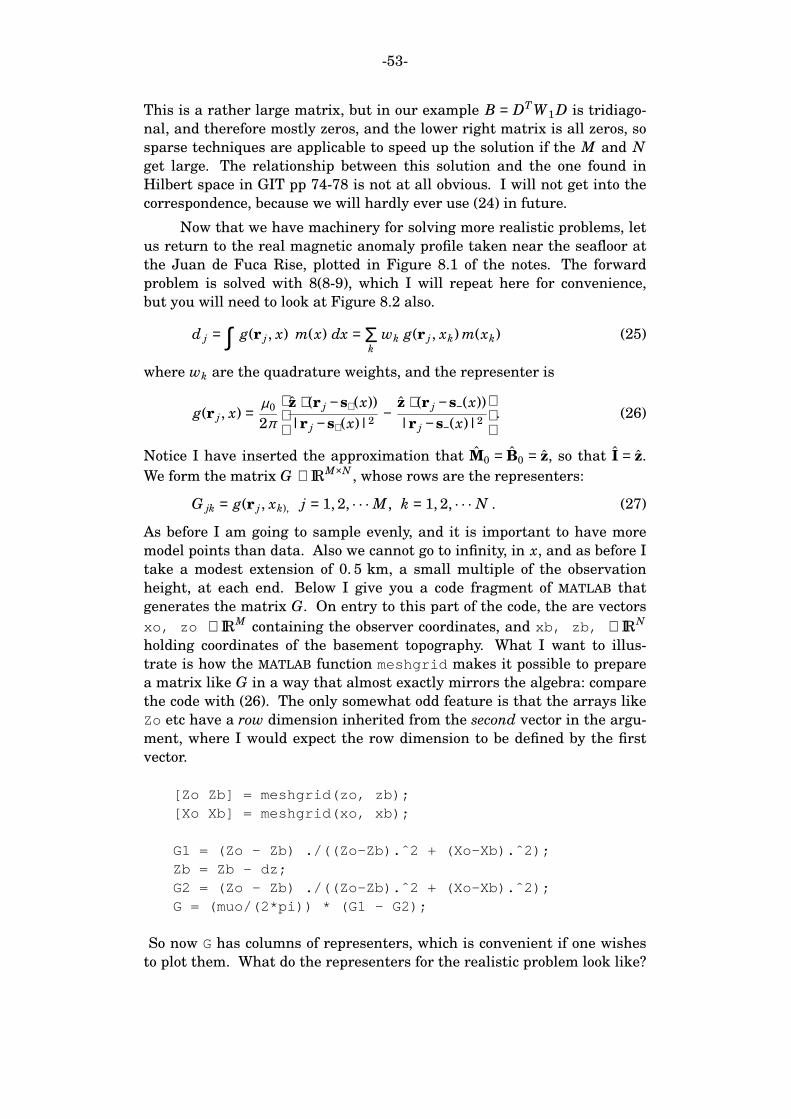
-53-
This is a rather large matrix, but in our example B = DTW1 D is tridiago-
nal, and therefore mostly zeros, and the lower right matrix is all zeros, so
sparse techniques are applicable to speed up the solution if the M and N
get large. The relationship between this solution and the one found in
Hilbert space in GIT pp 74-78 is not at all obvious. I will not get into the
correspondence, because we will hardly ever use (24) in future.
Now that we have machinery for solving more realistic problems, let
us return to the real magnetic anomaly profile taken near the seafloor at
the Juan de Fuca Rise, plotted in Figure 8.1 of the notes. The forward
problem is solved with 8(8-9), which I will repeat here for convenience,
but you will need to look at Figure 8.2 also.
d j = ∫ g(r j , x) m(x) dx =kΣ wk g(r j , xk) m(xk) (25)
where wk are the quadrature weights, and the representer is
g(r j , x) =µ0
2π
z ⋅ (r j −s+(x))
|r j −s+(x)|2−
z ⋅ (r j −s−(x))
|r j −s−(x)|2
. (26)
Notice I have inserted the approximation that M0 = B0 = z, so that I = z.
We form the matrix G ∈ IRM×N , whose rows are the representers:
G jk = g(r j , xk), j = 1, 2, . . . M, k = 1, 2, . . . N . (27)
As before I am going to sample evenly, and it is important to have more
model points than data. Also we cannot go to infinity, in x, and as before I
take a modest extension of 0. 5 km, a small multiple of the observation
height, at each end. Below I give you a code fragment of MATLAB that
generates the matrix G. On entry to this part of the code, the are vectors
xo, zo ∈ IRM containing the observer coordinates, and xb, zb, ∈ IRN
holding coordinates of the basement topography. What I want to illus-
trate is how the MATLAB function meshgrid makes it possible to prepare
a matrix like G in a way that almost exactly mirrors the algebra: compare
the code with (26). The only somewhat odd feature is that the arrays like
Zo etc have a row dimension inherited from the second vector in the argu-
ment, where I would expect the row dimension to be defined by the first
vector.
[Zo Zb] = meshgrid(zo, zb);[Xo Xb] = meshgrid(xo, xb);
G1 = (Zo - Zb) ./((Zo-Zb).ˆ2 + (Xo-Xb).ˆ2);Zb = Zb - dz;G2 = (Zo - Zb) ./((Zo-Zb).ˆ2 + (Xo-Xb).ˆ2);G = (muo/(2*pi)) * (G1 - G2);
So now G has columns of representers, which is convenient if one wishes
to plot them. What do the representers for the realistic problem look like?
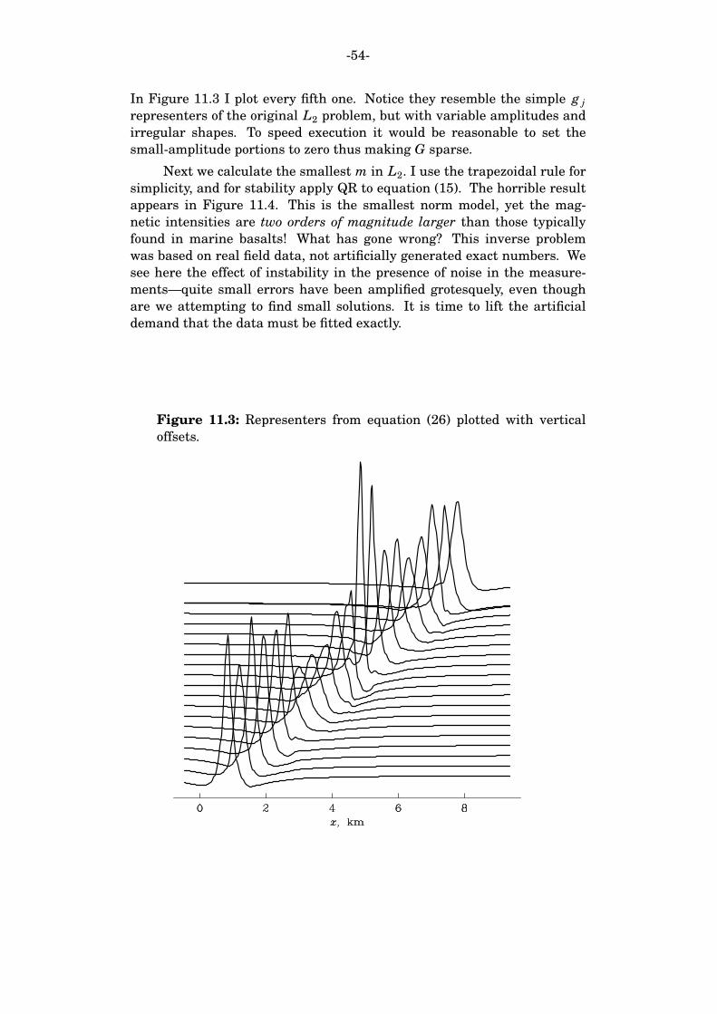
-54-
In Figure 11.3 I plot every fifth one. Notice they resemble the simple g j
representers of the original L2 problem, but with variable amplitudes and
irregular shapes. To speed execution it would be reasonable to set the
small-amplitude portions to zero thus making G sparse.
Next we calculate the smallest m in L2. I use the trapezoidal rule for
simplicity, and for stability apply QR to equation (15). The horrible result
appears in Figure 11.4. This is the smallest norm model, yet the mag-
netic intensities are two orders of magnitude larger than those typically
found in marine basalts! What has gone wrong? This inverse problem
was based on real field data, not artificially generated exact numbers. We
see here the effect of instability in the presence of noise in the measure-
ments—quite small errors have been amplified grotesquely, even though
are we attempting to find small solutions. It is time to lift the artificial
demand that the data must be fitted exactly.
Figure 11.3: Representers from equation (26) plotted with vertical
offsets.
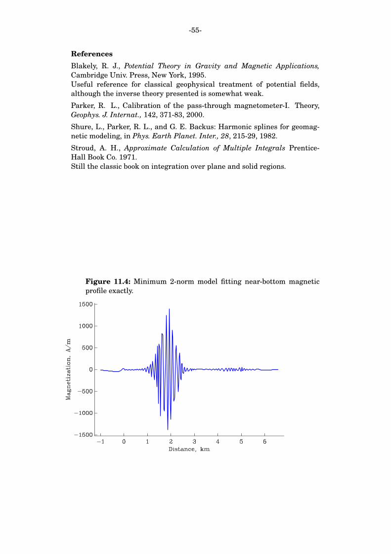
-55-
References
Blakely, R. J., Potential Theory in Gravity and Magnetic Applications,
Cambridge Univ. Press, New York, 1995.
Useful reference for classical geophysical treatment of potential fields,
although the inverse theory presented is somewhat weak.
Parker, R. L., Calibration of the pass-through magnetometer-I. Theory,
Geophys. J. Internat., 142, 371-83, 2000.
Shure, L., Parker, R. L., and G. E. Backus: Harmonic splines for geomag-
netic modeling, in Phys. Earth Planet. Inter., 28, 215-29, 1982.
Stroud, A. H., Approximate Calculation of Multiple Integrals Prentice-
Hall Book Co. 1971.
Still the classic book on integration over plane and solid regions.
Figure 11.4: Minimum 2-norm model fitting near-bottom magnetic
profile exactly.
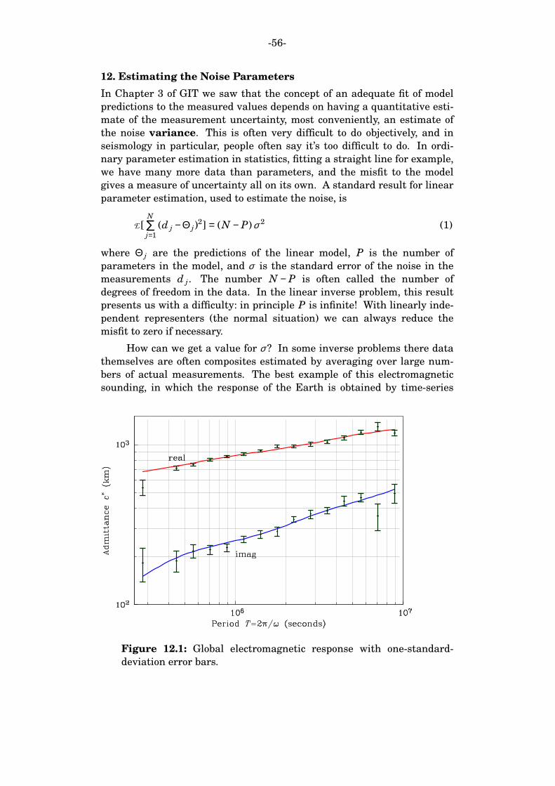
-56-
12. Estimating the Noise Parameters
In Chapter 3 of GIT we saw that the concept of an adequate fit of model
predictions to the measured values depends on having a quantitative esti-
mate of the measurement uncertainty, most conveniently, an estimate of
the noise variance. This is often very difficult to do objectively, and in
seismology in particular, people often say it’s too difficult to do. In ordi-
nary parameter estimation in statistics, fitting a straight line for example,
we have many more data than parameters, and the misfit to the model
gives a measure of uncertainty all on its own. A standard result for linear
parameter estimation, used to estimate the noise, is
E [N
j=1Σ (d j − Θ j)
2] = (N − P) σ 2 (1)
where Θ j are the predictions of the linear model, P is the number of
parameters in the model, and σ is the standard error of the noise in the
measurements d j . The number N − P is often called the number of
degrees of freedom in the data. In the linear inverse problem, this result
presents us with a difficulty: in principle P is infinite! With linearly inde-
pendent representers (the normal situation) we can always reduce the
misfit to zero if necessary.
How can we get a value for σ ? In some inverse problems there data
themselves are often composites estimated by averaging over large num-
bers of actual measurements. The best example of this electromagnetic
sounding, in which the response of the Earth is obtained by time-series
Figure 12.1: Global electromagnetic response with one-standard-
deviation error bars.
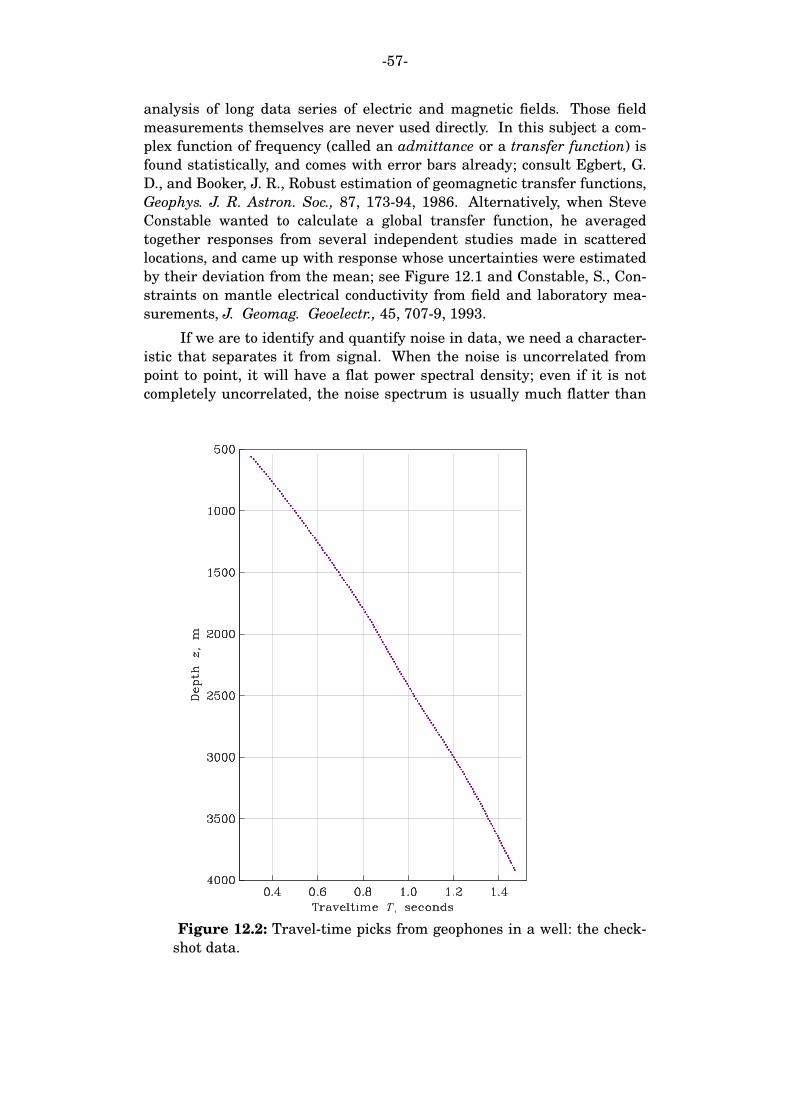
-57-
analysis of long data series of electric and magnetic fields. Those field
measurements themselves are never used directly. In this subject a com-
plex function of frequency (called an admittance or a transfer function) is
found statistically, and comes with error bars already; consult Egbert, G.
D., and Booker, J. R., Robust estimation of geomagnetic transfer functions,
Geophys. J. R. Astron. Soc., 87, 173-94, 1986. Alternatively, when Steve
Constable wanted to calculate a global transfer function, he averaged
together responses from several independent studies made in scattered
locations, and came up with response whose uncertainties were estimated
by their deviation from the mean; see Figure 12.1 and Constable, S., Con-
straints on mantle electrical conductivity from field and laboratory mea-
surements, J. Geomag. Geoelectr., 45, 707-9, 1993.
If we are to identify and quantify noise in data, we need a character-
istic that separates it from signal. When the noise is uncorrelated from
point to point, it will have a flat power spectral density; even if it is not
completely uncorrelated, the noise spectrum is usually much flatter than
Figure 12.2: Travel-time picks from geophones in a well: the check-
shot data.
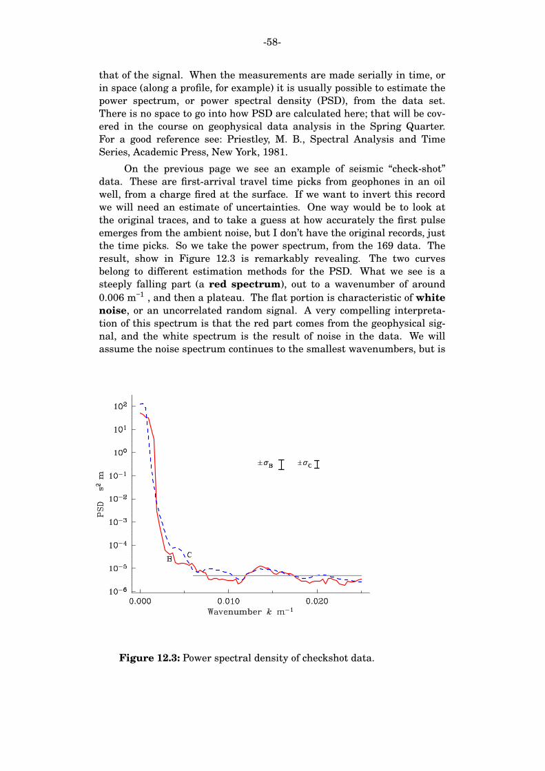
-58-
that of the signal. When the measurements are made serially in time, or
in space (along a profile, for example) it is usually possible to estimate the
power spectrum, or power spectral density (PSD), from the data set.
There is no space to go into how PSD are calculated here; that will be cov-
ered in the course on geophysical data analysis in the Spring Quarter.
For a good reference see: Priestley, M. B., Spectral Analysis and Time
Series, Academic Press, New York, 1981.
On the previous page we see an example of seismic ‘‘check-shot’’
data. These are first-arrival travel time picks from geophones in an oil
well, from a charge fired at the surface. If we want to invert this record
we will need an estimate of uncertainties. One way would be to look at
the original traces, and to take a guess at how accurately the first pulse
emerges from the ambient noise, but I don’t have the original records, just
the time picks. So we take the power spectrum, from the 169 data. The
result, show in Figure 12.3 is remarkably revealing. The two curves
belong to different estimation methods for the PSD. What we see is a
steeply falling part (a red spectrum), out to a wavenumber of around
0.006 m−1 , and then a plateau. The flat portion is characteristic of white
noise, or an uncorrelated random signal. A very compelling interpreta-
tion of this spectrum is that the red part comes from the geophysical sig-
nal, and the white spectrum is the result of noise in the data. We will
assume the noise spectrum continues to the smallest wavenumbers, but is
Figure 12.3: Power spectral density of checkshot data.
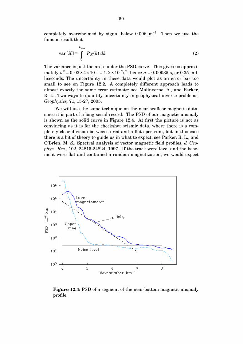
-59-
completely overwhelmed by signal below 0.006 m−1. Then we use the
famous result that
var [X ] =kmax
0
∫ P X (k) dk (2)
The variance is just the area under the PSD curve. This gives us approxi-
mately σ 2 = 0. 03 ×4 ×10−6 = 1. 2 ×10⁻⁷s2; hence σ = 0. 00035 s, or 0.35 mil-
liseconds. The uncertainty in these data would plot as an error bar too
small to see on Figure 12.2. A completely different approach leads to
almost exactly the same error estimate: see Malinverno, A., and Parker,
R. L., Two ways to quantify uncertainty in geophysical inverse problems,
Geophysics, 71, 15-27, 2005.
We will use the same technique on the near seafloor magnetic data,
since it is part of a long serial record. The PSD of our magnetic anomaly
is shown as the solid curve in Figure 12.4. At first the picture is not as
convincing as it is for the checkshot seismic data, where there is a com-
pletely clear division between a red and a flat spectrum, but in this case
there is a bit of theory to guide us in what to expect; see Parker, R. L., and
O’Brien, M. S., Spectral analysis of vector magnetic field profiles, J. Geo-
phys. Res., 102, 24815-24824, 1997. If the track were level and the base-
ment were flat and contained a random magnetization, we would expect
Figure 12.4: PSD of a segment of the near-bottom magnetic anomaly
profile.

-60-
the magnetic anomaly PSD to fall approximately exponentially, like
exp (−4πkh). The elevation of the magnetometer above the basement lies
roughly between 116 m and 200 m, and the lower level will dominate at
the higher wavenumbers; the long dashed line shows the exponential fall-
off for the lower value of h, and it fits the spectrum rather well. There is
a break at about 6 km−1, which I will interpret as the point where noise
begins to exceed signal. In marine magnetic surveys the noise is caused
by other environmental magnetic fields, such as time-varying fields due to
currents in the ionosphere, and also those from electric currents in the
water caused by induction. I will assume the PSD of the noise is approxi-
mately white, and follows the horizontal grey line. The corresponding
variance from (2) is 8. 5 × 25 = 210 nT2 which yields a value for
σ = 14. 5 nT. Remarkable confirmation for this model comes from the sec-
ond PSD, shown with short dashes. Unusually in a survey of this kind, a
second magnetometer was tethered to the cable 300 m higher up than the
one we have been using. By the theory I mentioned, its spectrum falls
much faster, so the PSD hits the noise level at a lower wavenumber, and
as we see in the figure, it levels out at the same value, because it is in
essentially the same noise environment as the lower instrument. Thanks
to the second magnetometer we can be confident in our estimate for the
uncertainty.
The spectral approach requires a number of additional assumptions
about the noise, primarily, that it is statistically stationary. This means
that the random process responsible for the noise is the same everywhere
in the data series. That is often a plausible assumption, and would be
accepted for the marine data. The message I want to leave you with is
that the power spectrum usually gives an important clue about the noise,
because the noise persists out to the highest frequencies, while most natu-
ral processes have a red spectrum, and the components of the signal at
the high frequencies (or wavenumbers) are usually attenuated, thus per-
mitted the noise spectrum to show itself. If this doesn’t happen the data
are not being sampled at a high enough rate, and there is danger of alias-
ing, which means the signal is being sampled too slowly to capture its
true behavior.

-61-
References
Constable, S., Constraints on mantle electrical conductivity from field and
laboratory measurements, J. Geomag. Geoelectr., 45, 707-9, 1993.
Egbert, G. D., and Booker, J. R., Robust estimation of geomagnetic trans-
fer functions, Geophys. J. R. Astron. Soc., 87, 173-94, 1986.
Malinverno, A., and Parker, R. L., Two ways to quantify uncertainty in
geophysical inverse problems, Geophysics, 71, 15-27, 2005.
Parker, R. L., Coherence of signals from magnetometers on parallel paths,
J. Geophys. Res., 102, 5111-7, 1997.
Parker, R. L., and O’Brien, M. S., Spectral analysis of vector magnetic
field profiles, J. Geophys. Res., 102, 24815-24824, 1997.
Priestley, M. B.,Spectral Analysis and Time Series, Academic Press, New
York, 1981.
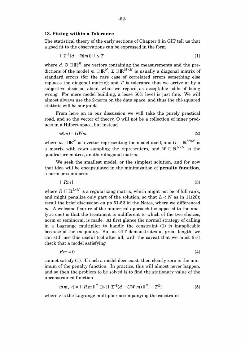
-62-
13. Fitting within a Tolerance
The statistical theory of the early sections of Chapter 3 in GIT tell us that
a good fit to the observations can be expressed in the form
||Σ−1(d − Θ(m))|| ≤ T (1)
where d, Θ ∈ IRM are vectors containing the measurements and the pre-
dictions of the model m ∈ IRN ; Σ ∈ IRM×M is usually a diagonal matrix of
standard errors (for the rare case of correlated errors something else
replaces the diagonal matrix); and T is tolerance that we arrive at by a
subjective decision about what we regard as acceptable odds of being
wrong. For mere model building, a loose 50% level is just fine. We will
almost always use the 2-norm on the data space, and thus the chi-squared
statistic will be our guide.
From here on in our discussion we will take the purely practical
road, and so the vector of theory, Θ will not be a collection of inner prod-
ucts in a Hilbert space, but instead
Θ(m) = GWm (2)
where m ∈ IRN is a vector representing the model itself, and G ∈ IRM×N is
a matrix with rows sampling the representers, and W ∈ IRN×N is the
quadrature matrix, another diagonal matrix.
We seek the smallest model, or the simplest solution, and for now
that idea will be encapsulated in the minimization of penalty function,
a norm or seminorm:
||Rm|| (3)
where R ∈ IRL×N is a regularizing matrix, which might not be of full rank,
and might penalize only part of the solution, so that L < N as in 11(20);
recall the brief discussion on pp 51-52 in the Notes, where we differenced
m. A welcome feature of the numerical approach (as opposed to the ana-
lytic one) is that the treatment is indifferent to which of the two choices,
norm or seminorm, is made. At first glance the normal strategy of calling
in a Lagrange multiplier to handle the constraint (1) is inapplicable
because of the inequality. But as GIT demonstrates at great length, we
can still use this useful tool after all, with the caveat that we must first
check that a model satisfying
Rm = 0 (4)
cannot satisfy (1). If such a model does exist, then clearly zero is the min-
imum of the penalty function. In practice, this will almost never happen,
and so then the problem to be solved is to find the stationary value of the
unconstrained function
u(m, ν ) = ||R m||2 + ν [||Σ−1(d − GW m)||
2] − T2] (5)
where ν is the Lagrange multiplier accompanying the constraint:
-63-
||Σ−1(d − GW m)|| = T . (6)
To reduce the clutter I introduce a couple of abbreviations: let
d = Σ−1d, and B = Σ−1GW . (7)
This gives us the new unconstrained function
u(m,ν ) = ||R m||2 + ν [||d − B m||
2] − T2] . (8)
Notice that, for a fixed value of T , minimization of this expression can be
regarded as seeking a compromise between two undesirable properties of
the solution: the first term represents model complexity, which we wish to
keep small; the second measures model misfit, also a quantity to be sup-
pressed as far as possible. By making ν > 0 but small we pay attention to
the penalty function at the expense of data misfit, while making ν large
works in the other direction, and allows large penalty values to secure a
good match to observation. Let us continue.
We can differentiate (8) with respect to m by writing out the expres-
sion in terms of components; I will spare you the intermediate steps
which we have seen several times in slightly different contexts. At a sta-
tionary point of (8) the gradient of u vanishes and we find the vector m0
obeys
RT R m0 + ν BT B m0 − ν BT d = 0 . (9)
Or, equivalently, m0 satisfies the linear system
(BT B +1
νRT R) m0 = BT d . (10)
Differentiating with ν returns the constraint, now written as
||d − B m0|| = T . (11)
If we knew the value of ν , we could find the model by solving (10). So the
tactic for solving (10) and (11) together, as we must, requires solving (10)
for a sequence of ν s seeking the vector m0 that gives (11). We need to
show that as ν increases, the misfit norm in (11) decreases. This result is
intuitive from our discussion after (8), but it also is useful to have the de-
rivative itself. Consider the squared misfit in (11) to be purely a function
of ν :
F(ν ) = ||d − B m0(ν )||2
. (12)
Then differentiating on ν
dF
dν= − 2 (d − B m0(ν ))T B
dm0
dν= −2 (BT (d − B m0))T dm0
dν. (13)
By rearranging (9) we see that
BT (d − B m0) =1
νRT Rm0 (14)
-64-
and hence
dF
dν= −
2
ν(RT Rm0)T dm0
dν. (15)
Now to get dm0/dν , differentiate both sides of (10):
(BT B +1
νRT R)
dm0
dν−
1
ν 2RT Rm0 = 0 . (16)
Solving for dm0/dν and plugging the answer into (15) gives the glorious
result
dF
dν= −
2
ν 3(RT Rm0)T (BT B +
1
νRT R)−1(RT Rm0) . (17)
The inverse matrix in the middle is positive definite, because it is com-
posed of the sum of positive definite pieces; then, since ν > 0 the whole
thing must be negative.
This simplifies the strategy for solving the pair (10)-(11), because
now we know that when a guess for ν yields a value of F that is too high,
we must increase ν , and conversely. Better yet we can even use Newton’s
method, which you will recall can be used for solving equations in a sin-
gle variable: in this case the equation is
F(ν 0) = T2 . (18)
We begin with an initial value ν 1 > 0, and we perform a one-term Taylor
expansion on (18) as follows:
T2 = F(ν 1 +ν 0 −ν 1) = F(ν 1) + (ν 0 −ν 1)F ′(ν 1) + ε (19)
where F ′ denotes the derivative, and ε is error due to the neglect of higher
order terms in the series. Rearranging this expression gives
ν 0 = ν 1 −F(ν 1) − T2
F ′(ν 1)+
εF ′(ν 1)
. (20)
If the ε , the second order term in the Taylor expansion is neglected, (20)
gives a recipe for the next step in an iterative process which we write
ν n+1 = ν n −F(ν n) − T2
F ′(ν n), n = 1, 2, . . . . (21)
It is shown in GIT that this procedure always converges, provided the ini-
tial guess obeys ν 1<ν 0. But surprisingly perhaps, a faster rate of conver-
gence is usually obtained by writing (18) as
ln (F(ν 0)) = 2 ln T (22)
and solving this equation with Newton’s method.
Let us summarize the process. Recall the abbreviations introduced
in (7). We wish to discover the solution vector m0 and the Lagrange mul-
tiplier ν 0 which solve simultaneously the linear system (10) and the misfit
constraint (11). We make an initial guess for ν which we call ν 1, and with
-65-
it we solve (10). We take the resultant model vector and put it into (12)
which gives us F. We also solve the system (17), which provides us with
dF/dν . If F is close enough to T2 we stop. Otherwise we use (21) to
obtain a revised version of ν , with which we can begin the cycle again.
There are a number of points, before we examine this process in an
illustration. Equation (10) can be written as the solution to an overdeter-
mined least-squares approximation problem:
B
ν −½ R
m0 ∼
d
0
(23)
you will easily verify that the normal equations for this overdetermined
least squares problem is exactly (10). We can write a similar equation for
dm0/dν
B
ν −½ R
dm0
dν∼
0
ν −3/2 Rm0
(24)
There are two possible reasons for treating (10) as the solution of (23).
First, when the size of the system is modest, we can solve (23) by QR fac-
torization and avoid poor numerical stability. Second, R is almost always
sparse, so when the system is large we can take advantage of the sparse
LS form of the solution, 6(13) in our notes on linear algebra. And if the
system is very large, that form can be conveniently solved by the method
of conjugate gradients, as we will see later.
Let us now apply this approach to our near-bottom magnetic anom-
aly problem. You may recall that we looked for the smallest magnetiza-
tion model in L2 that fit the measured values exactly and obtained a
mess, plotted in Figure 11.4. The model is one hundred times larger than
a reasonable solution should be, yet it is the smallest model. The fault is
the demand of an exact fit. In Section 11 of these Notes I obtained a noise
estimate of σ = 14. 5 nT, a quantity too small to be distinguished in a plot
showing the full range of the data; can such a small misfit reduce the size
of the solution to a reasonable level? We decide in advance what will be
acceptable as a plausible size of misfit. I suggest that we take the
expected value of error norm as a trial value. Thus, as shown in GIT on p
124
E [||d − Θ||/σ ] = √ N [1 −1
4N+ . . .] (25)
where we have used the fact that noise will be treated as iid. Then since
N = 100, we calculate that the misfit tolerance in 11(6) is T = 9. 975. The
target misfit for Newton’s method is T2. We will minimize the L2 norm as
before, using trapezoidal rule for all the integrations.
In the figure on the next page we see the progress of the iterative
solution, which starts with ν = 0. 001 and then goes down in F and up in
ν . The starting guess lies below the solution ν 0, and so Newton is
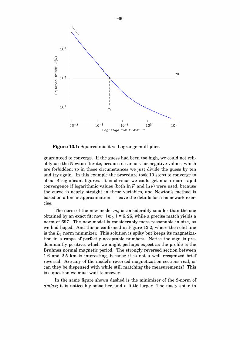
-66-
Figure 13.1: Squared misfit vs Lagrange multiplier.
guaranteed to converge. If the guess had been too high, we could not reli-
ably use the Newton iterate, because it can ask for negative values, which
are forbidden; so in those circumstances we just divide the guess by ten
and try again. In this example the procedure took 10 steps to converge to
about 4 significant figures. It is obvious we could get much more rapid
convergence if logarithmic values (both ln F and lnν ) were used, because
the curve is nearly straight in these variables, and Newton’s method is
based on a linear approximation. I leave the details for a homework exer-
cise.
The norm of the new model m0 is considerably smaller than the one
obtained by an exact fit: now ||m0|| = 6. 26, while a precise match yields a
norm of 697. The new model is considerably more reasonable in size, as
we had hoped. And this is confirmed in Figure 13.2, where the solid line
is the L2 norm minimizer. This solution is spiky but keeps its magnetiza-
tion in a range of perfectly acceptable numbers. Notice the sign is pre-
dominantly positive, which we might perhaps expect as the profile is the
Bruhnes normal magnetic period. The strongly reversed section between
1.6 and 2.5 km is interesting, because it is not a well recognized brief
reversal. Are any of the model’s reversed magnetization sections real, or
can they be dispensed with while still matching the measurements? This
is a question we must wait to answer.
In the same figure shown dashed is the minimizer of the 2-norm of
dm/dx; it is noticeably smoother, and a little larger. The nasty spike in
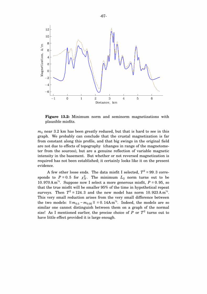
-67-
Figure 13.2: Minimum norm and seminorm magnetizations with
plausible misfits.
m0 near 3.2 km has been greatly reduced, but that is hard to see in this
graph. We probably can conclude that the crustal magnetization is far
from constant along this profile, and that big swings in the original field
are not due to effects of topography (changes in range of the magnetome-
ter from the sources), but are a genuine reflection of variable magnetic
intensity in the basement. But whether or not reversed magnetization is
required has not been established; it certainly looks like it on the present
evidence.
A few other loose ends. The data misfit I selected, T2 = 99. 3 corre-
sponds to P = 0. 5 for χ 2N . The minimum L2 norm turns out to be
10. 970 A m½. Suppose now I select a more generous misfit, P = 0. 95, so
that the true misfit will be smaller 95% of the time in hypothetical repeat
surveys. Then T2 = 124. 3 and the new model has norm 10. 923 A m½.
This very small reduction arises from the very small difference between
the two models: ||m0.5 − m0.95|| = 0. 14A m½. Indeed, the models are so
similar one cannot distinguish between them on a graph of the normal
size! As I mentioned earlier, the precise choice of P or T2 turns out to
have little effect provided it is large enough.
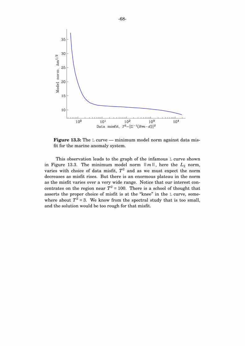
-68-
Figure 13.3: The L curve — minimum model norm against data mis-
fit for the marine anomaly system.
This observation leads to the graph of the infamous L curve shown
in Figure 13.3. The minimum model norm ||m||, here the L2 norm,
varies with choice of data misfit, T2 and as we must expect the norm
decreases as misfit rises. But there is an enormous plateau in the norm
as the misfit varies over a very wide range. Notice that our interest con-
centrates on the region near T2 = 100. There is a school of thought that
asserts the proper choice of misfit is at the ‘‘knee’’ in the L curve, some-
where about T2 = 3. We know from the spectral study that is too small,
and the solution would be too rough for that misfit.

-69-
14. Resolution in the Marine Magnetics Example
We carry out the resolution analysis for the model on the Juan de Fuca
Ridge that has been our standard vehicle in the linear theory. As
explained in class, one of the fairly traditional ways of doing this is to cali-
brate the regularization process by testing it with artificial data, gener-
ated from special models, often delta functions, at various points. This
must be done using exactly the same parameter settings as were used in
making the regularized model. Then we see at each point how badly
smeared out a very sharp feature would be after being processed through
the inversion machinery. This gives us a qualitative assessment of the
length scales resolved in the solution.
Figure 14.1 shows the results for five locations of the test function.
We see the resolution varies by quite a large factor from place to place,
but is reasonably satisfactory everywhere. At x = 2 km we may be resolv-
ing structure only down to about 0.5 km, while near 3 km the resolution
improves to almost 0.1 km. The cause of the variation is easy to discover
in this case: resolving scale is apparently proportional to the distance to
the nearest source material, as you can easily see by comparing this fig-
ure with Figure 8.1.
Figure 14.1: Top: L2-norm minimizing magnetization. Bottom: Reso-
lution functions for various sites.

-70-
15. Practical Calculation of a Bound
In Section 4.03 of GIT I treat the question of finding the range of a linear
functional subject to constraints from data (linear functions) and a nonlin-
ear conditions, that the norm be restricted as well. There in the noise-free
case an elegant theory is developed for the noise-free case (data matched
exactly by the model), and a number of predictions, also in the form of lin-
ear functionals. The problem with noise seems to be much more clumsy.
Here I want to give a simpler for numerically formulated problems.
To motivate the discussion look again at Figure 14.1 and the nega-
tive magnetization near x = 2 km. According to the resolution calcula-
tions, the regularized model should be trustworthy on the scale of a kilo-
meter, and so we are inclined to accept the reality of reversed magnetiza-
tion in this region. But is that truly required by the data? As GIT 4.03
shows us, we cannot be sure without introducing some further informa-
tion. Suppose we say we know the L2 norm of m. If we confine all mag-
netic material to −0. 5 ≤ x ≤ 6 then ||m||/√ 6. 5 = MRMS, and we might be
willing to specify an upper limit on plausible RMS magnetizations, from
samples of fresh marine basalts. Then one way we might answer the
question of a possible record of magnetic reversal is to consider the aver-
age value of magnetization over the x interval (x1, x2) where the regular-
ized model dips negative; numerically this is (1.8, 2.4) km. We will call
this <m>:
<m> =1
x2 − x1
x2
x1
∫ m(x) dx . (1)
We challenge the hypothesis that the negative <m> is required: if the
every model that adequately matches the anomalies and has a positive
average possesses an implausibly large RMS magnetization then a rever-
sal is demanded in the interval. The converse, a positive average consis-
tent with a reasonable RMS, does not mean the absence of a reversal how-
ever, because negative segments might still be needed, even with a posi-
tive average—it is just an average; we’ll return to this later.
The idea then is to seek the smallest norm of the discretized model
m ∈ IRN :
m ∈ IRNmin ||Rm|| (2)
subject to an adequate fit to the measurements:
||d − B m|| ≤ T (3)
and the constraint on a linear functional of the model, in the example the
average given in (1):
lT m = b (4)
where the scaled data d and matrix B ∈ IRM×N are given in 13(8); l ∈ IRN
-71-
is vector which approximates averaging the model over a region. If the
smallest norm found in (2) is too large when (2) and (3) hold, we know
that (3) cannot be supported. How does one apply the equality constraint
(4)? Obviously one approach is introduce a second Lagrange multiplier, in
addition to the one needed to account for (3). Let me describe a simpler
approach. We treat (4) as another fictitious "observation" to be fitted
(almost) exactly by including it in (3). Write a data vector d1 ∈ IRN+1 and
a new B1 ∈ IR(M+1)×N and a scalar γ :
B1 =
γ lT
B
; d1 =
γ b
d
(5)
where γ > 0 is a very large constant. This clearly has the effect in the fit-
ting problem of giving (4) a heavy weight, so that it will be fit more accu-
rately than the rest of the data. Now we solve the standard norm mini-
mization problem (2) subject to misfit (3) achieving a specified tolerance
exactly as in (3), where B and d are replaced by B1 and d1. But wait a
minute—shouldn’t we have to designate a new T as well? We have
messed up the fitting process by including a very accurate fake datum.
The answer is no: it can be shown (in Chapter 22, of Solving Least
Squares Problems, by Lawson and Hanson, 1974) that if γ is large enough,
the misfit component introduced by the new row in B1 is negligible! How
large is that? Lawson and Hanson give a very conservative figure; I find
that if γ ||l|| = 100||B|| we can get very good results. Too large a value
for γ leads to numerical instability, unfortunately. The advantage of this
approach is that we use exactly the same code when we bound the linear
function l as when we find a regularized model.
We apply these ideas to the near-bottom magnetic anomalies. The
linear functional we are interested in is the average value <m> in the
interval where the regularized model goes negative, so if the length of
that interval is D = x2 − x1 and the spacing in the discretized model is ∆x,
the vector l in (4) looks like this if we use the trapezoidal rule to approxi-
mate (1):
l =∆x
D[0, 0, . . . 0, ½, 1, 1, 1, 1, . . . 1, ½, 0, 0, . . . 0]T . (6)
The first choice for b the bound in (4) might be zero, but in fact consider-
able insight is gained if we sweep b through a range of values. The
results are plotted in Figure 15.1. For each value of <m> we plot the min-
imum possible norm, normalized to be RMS magnetization. That means
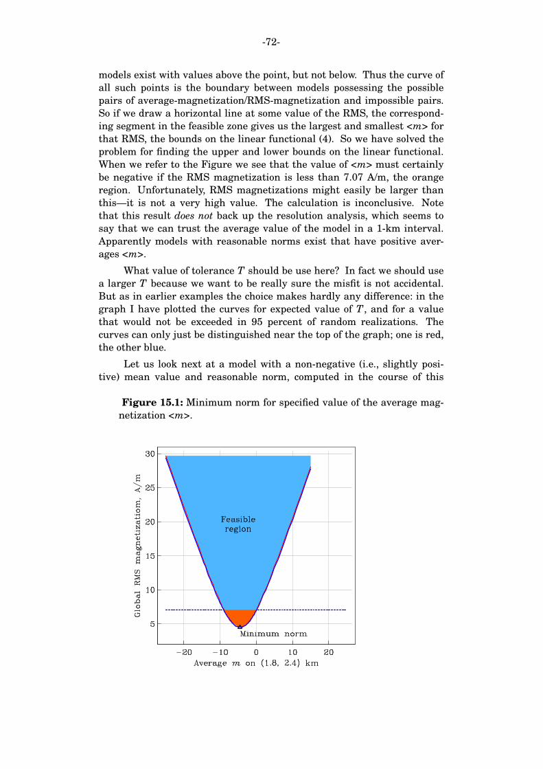
-72-
models exist with values above the point, but not below. Thus the curve of
all such points is the boundary between models possessing the possible
pairs of average-magnetization/RMS-magnetization and impossible pairs.
So if we draw a horizontal line at some value of the RMS, the correspond-
ing segment in the feasible zone gives us the largest and smallest <m> for
that RMS, the bounds on the linear functional (4). So we have solved the
problem for finding the upper and lower bounds on the linear functional.
When we refer to the Figure we see that the value of <m> must certainly
be negative if the RMS magnetization is less than 7.07 A/m, the orange
region. Unfortunately, RMS magnetizations might easily be larger than
this—it is not a very high value. The calculation is inconclusive. Note
that this result does not back up the resolution analysis, which seems to
say that we can trust the average value of the model in a 1-km interval.
Apparently models with reasonable norms exist that have positive aver-
ages <m>.
What value of tolerance T should be use here? In fact we should use
a larger T because we want to be really sure the misfit is not accidental.
But as in earlier examples the choice makes hardly any difference: in the
graph I have plotted the curves for expected value of T , and for a value
that would not be exceeded in 95 percent of random realizations. The
curves can only just be distinguished near the top of the graph; one is red,
the other blue.
Let us look next at a model with a non-negative (i.e., slightly posi-
tive) mean value and reasonable norm, computed in the course of this
Figure 15.1: Minimum norm for specified value of the average mag-
netization <m>.

-73-
Figure 15.2: Model with reasonable RMS, fitting the data, and pos-
sessing a positive mean <m> = 1 A/m. The L2 norm minimizer is
shown light.
solution. The model with <m> = 1 A/m and RMS value 8.2 A/m is shown
in Figure 15.2. Despite having an overall positive average over the inter-
val of interest, the function is still negative in places, and a reversed mag-
netization is required. Furthermore, the model has large peak values,
both negative and positive that make it seem unreasonable. Particularly
troubling are the large negative swings, just outside the averaging inter-
val. All of this strongly suggests that in this problem the use of the aver-
age value to test a hypothesis is not very effective. If we could test the
hypothesis that any magnetization that is positive everywhere on the
interval will not fit the data, then we might have a really strong test.
That is the direction we are heading.
We have been pursuing the possibility that our magnetic data may
demand a reversely magnetized section of crust, which would be quite
interesting if it turned out to be true; in fact, because such a reversed seg-
ment has not been documented elsewhere, we want to be particularly cer-
tain it is required. So far, the evidence is not convincing. A reason pecu-
liar to marine magnetic studies, is the very small response of the system
to long wavelength magnetizations. Recall from Section 9, in the ideal-
ized case of a flat layer and horizontal observation track, a constant mag-
netization is completely invisible in the data: then (g j , c) = 0 for
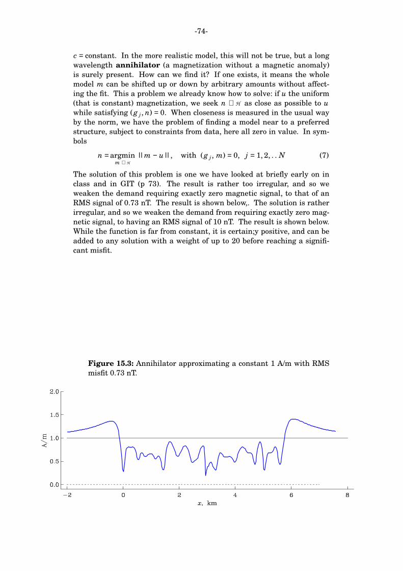
-74-
c = constant. In the more realistic model, this will not be true, but a long
wa velength annihilator (a magnetization without a magnetic anomaly)
is surely present. How can we find it? If one exists, it means the whole
model m can be shifted up or down by arbitrary amounts without affect-
ing the fit. This a problem we already know how to solve: if u the uniform
(that is constant) magnetization, we seek n ∈ H as close as possible to u
while satisfying (g j , n) = 0. When closeness is measured in the usual way
by the norm, we have the problem of finding a model near to a preferred
structure, subject to constraints from data, here all zero in value. In sym-
bols
n =m ∈ H
argmin ||m − u||, with (g j , m) = 0, j = 1, 2, . . N (7)
The solution of this problem is one we have looked at briefly early on in
class and in GIT (p 73). The result is rather too irregular, and so we
weaken the demand requiring exactly zero magnetic signal, to that of an
RMS signal of 0.73 nT. The result is shown below,. The solution is rather
irregular, and so we weaken the demand from requiring exactly zero mag-
netic signal, to having an RMS signal of 10 nT. The result is shown below.
While the function is far from constant, it is certain;y positive, and can be
added to any solution with a weight of up to 20 before reaching a signifi-
cant misfit.
Figure 15.3: Annihilator approximating a constant 1 A/m with RMS
misfit 0.73 nT.

-75-
16. NNLS and BVLS
Linear programming is able to solve linear inverse problems, with
inequality constraints imposed, provided we can tolerate a different norm
for measuring the misfit between model predictions and observations.
While the sup norm || ⋅ ||∞ and || ⋅ ||1 can both be treated in the LP set-
ting, only the latter is really useful, because relying on the sup norm gives
too much leverage to the noisiest data, clearly an inadvisable state of
affairs. To exploit a quadratic measure of misfit, like the familiar
X [m]2 =M
j=1Σ
(d j − L j[m])2
σ 2j
(1)
requires us to consider Quadratic Programming. Those QP problems
which are convex are much easier to solve reliably than the non-convex
ones, and I shall concentrate on two special convex cases that I have
found invaluable in my scientific career. First, is the special QP problem
called Non-Negative Least Squares (NNLS). This is simply the regular
least-squares problem with the positivity constraint attached:
x∗ = argx ≥ 0min ||Ax − y||2 (2)
where this notation, used extensively in the optimization literature,
means that x∗ is the vector x that achieves the minimum value (assuming
it is unique); here x, x∗ ∈ IRN , y ∈ IRM , and A ∈ IRM×N . In (2) there is no
restriction on the relative sizes of M and N ; the problem is interesting
and nontrivial whether N > M, which is the natural geophysical situation,
or not. There is a general property of optimization problems, somewhat
similar to the Fundamental Theorem of LP called the Kuhn-Tucker condi-
tions, which in NNLS leads to an interesting and valuable result: a solu-
tion to (2) exists in which no more than M −1 components of x∗ are posi-
tive (and so by implication, at least N − M +1 of them must be zero, when
M < N ). When the dimension of the model space is large, as it will be in a
discretized version of a continuous problem, this means the same thing as
it did in the LP examples, that the solution vector x is mostly zeroes, with
a few positive spikes, delta functions in the limit of a continuum. In many
practical problems we find that the number of positive elements in the
solution vector, while it can be as large s M −1, often much smaller than
M.
Let me give a little graphical demonstration of the ideas as illus-
trated in Figure 16.1, which I will explain. First, consider the domain of
the solution set in RN , the set x ≥ 0, called the positive orthant. It is a
convex region in the space, whose edges comprise the positive extensions
of all the positive unit vectors. In three dimensions, the edges of the posi-
tive orthant (called the positive octant in IR3) are the positive x, y, and z
axes. Now consider mapping the positive orthant into RM with the linear
map A, where we will assume that M < N . The image of the orthant will
be a fan-shaped region as shown in the Figure, where M = 2 and N = 4.
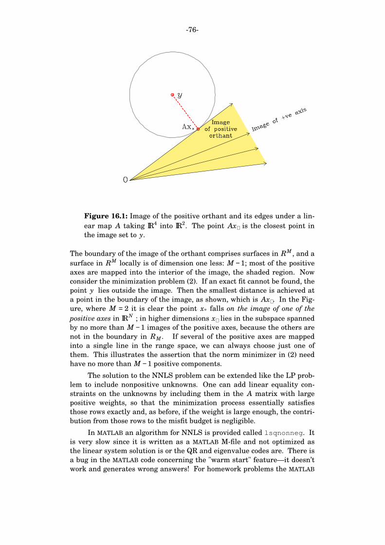
-76-
Figure 16.1: Image of the positive orthant and its edges under a lin-
ear map A taking IR4 into IR2. The point Ax∗ is the closest point in
the image set to y.
The boundary of the image of the orthant comprises surfaces in RM , and a
surface in RM locally is of dimension one less: M −1; most of the positive
axes are mapped into the interior of the image, the shaded region. Now
consider the minimization problem (2). If an exact fit cannot be found, the
point y lies outside the image. Then the smallest distance is achieved at
a point in the boundary of the image, as shown, which is Ax∗ . In the Fig-
ure, where M = 2 it is clear the point x* falls on the image of one of the
positive axes in IRN ; in higher dimensions x∗ lies in the subspace spanned
by no more than M −1 images of the positive axes, because the others are
not in the boundary in RM . If several of the positive axes are mapped
into a single line in the range space, we can always choose just one of
them. This illustrates the assertion that the norm minimizer in (2) need
have no more than M −1 positive components.
The solution to the NNLS problem can be extended like the LP prob-
lem to include nonpositive unknowns. One can add linear equality con-
straints on the unknowns by including them in the A matrix with large
positive weights, so that the minimization process essentially satisfies
those rows exactly and, as before, if the weight is large enough, the contri-
bution from those rows to the misfit budget is negligible.
In MATLAB an algorithm for NNLS is provided called lsqnonneg . It
is very slow since it is written as a MATLAB M-file and not optimized as
the linear system solution is or the QR and eigenvalue codes are. There is
a bug in the MATLAB code concerning the "warm start" feature—it doesn’t
work and generates wrong answers! For homework problems the MATLAB
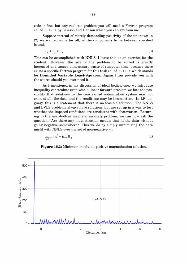
-77-
code is fine, but any realistic problem you will need a Fortran program
called nnls.f by Lawson and Hanson which you can get from me.
Suppose instead of merely demanding positivity of the unknown in
(2) we wanted some (or all) of the components to lie between specified
bounds:
l j ≤ x j ≤ u j (3)
This can be accomplished with NNLS; I leave this as an exercise for the
student. However, the size of the problem to be solved is greatly
increased and causes unnecessary waste of computer time, because there
exists a specific Fortran program for this task called bvls.f which stands
for Bounded Variable Least-Squares. Again I can provide you with
the source should you ever need it.
As I mentioned in my discussion of ideal bodies, once we introduce
inequality constraints even with a linear forward problem we face the pos-
sibility that solutions to the constrained optimization system may not
exist at all; the data and the conditions may be inconsistent. In LP lan-
guage this is a statement that there is no feasible solution. The NNLS
and BVLS problems always have solutions, but are set up in a way to test
whether the imposed conditions are consistent with observation. Return-
ing to the near-bottom magnetic anomaly problem, we can now ask the
question, "Are there any magnetization models that fit the data without
going negative somewhere?" This we do by simply minimizing the data
misfit with NNLS over the set of non-negative m:
m ≥ 0min ||d − Bm||2 (4)
Figure 16.2: Minimum misfit, all positive magnetization solution.
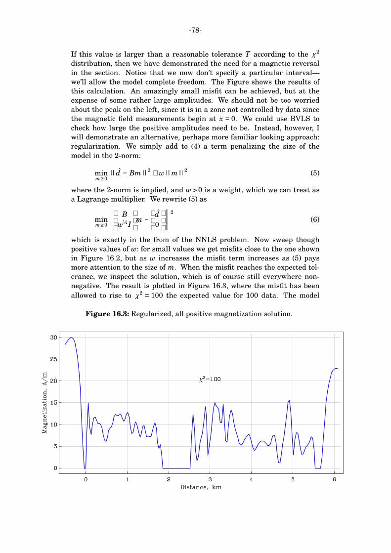
-78-
If this value is larger than a reasonable tolerance T according to the χ 2
distribution, then we have demonstrated the need for a magnetic reversal
in the section. Notice that we now don’t specify a particular interval—
we’ll allow the model complete freedom. The Figure shows the results of
this calculation. An amazingly small misfit can be achieved, but at the
expense of some rather large amplitudes. We should not be too worried
about the peak on the left, since it is in a zone not controlled by data since
the magnetic field measurements begin at x = 0. We could use BVLS to
check how large the positive amplitudes need to be. Instead, however, I
will demonstrate an alternative, perhaps more familiar looking approach:
regularization. We simply add to (4) a term penalizing the size of the
model in the 2-norm:
m ≥ 0min ||d − Bm||
2 + w||m||2
(5)
where the 2-norm is implied, and w > 0 is a weight, which we can treat as
a Lagrange multiplier. We rewrite (5) as
m ≥ 0min
B
w½ I
m −
d
0
2
(6)
which is exactly in the from of the NNLS problem. Now sweep though
positive values of w: for small values we get misfits close to the one shown
in Figure 16.2, but as w increases the misfit term increases as (5) pays
more attention to the size of m. When the misfit reaches the expected tol-
erance, we inspect the solution, which is of course still everywhere non-
negative. The result is plotted in Figure 16.3, where the misfit has been
allowed to rise to χ 2 = 100 the expected value for 100 data. The model
Figure 16.3: Regularized, all positive magnetization solution.

-79-
magnetizations are not extraordinary, and we must conclude that there
are reasonable-looking solutions without negative segments: the reversed
magnetization is not demanded by these data.
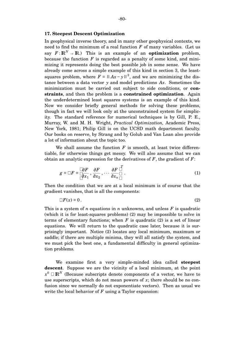
-80-
17. Steepest Descent Optimization
In geophysical inverse theory, and in many other geophysical contexts, we
need to find the minimum of a real function F of many variables. (Let us
say F : IRN → IR.) This is an example of an optimization problem,
because the function F is regarded as a penalty of some kind, and mini-
mizing it represents doing the best possible job in some sense. We have
already come across a simple example of this kind in section 3, the least-
squares problem, where F = ||Ax − y||2, and we are minimizing the dis-
tance between a data vector y and model predictions Ax. Sometimes the
minimization must be carried out subject to side conditions, or con-
straints, and then the problem is a constrained optimization. Again
the underdetermined least squares systems is an example of this kind.
Now we consider briefly general methods for solving these problems,
though in fact we will look only at the unconstrained system for simplic-
ity. The standard reference for numerical techniques is by Gill, P. E.,
Murray, W. and M. H. Wright, Practical Optimization, Academic Press,
New York, 1981; Philip Gill is on the UCSD math department faculty.
Our books on reserve, by Strang and by Golub and Van Loan also provide
a lot of information about the topic too.
We shall assume the function F is smooth, at least twice differen-
tiable, for otherwise things get messy. We will also assume that we can
obtain an analytic expression for the derivatives of F, the gradient of F:
g = ∇ F =
∂F
∂x1
,∂F
∂x2
, . . .∂F
∂xn
T
. (1)
Then the condition that we are at a local minimum is of course that the
gradient vanishes, that is all the components:
∇ F(x) = 0 . (2)
This is a system of n equations in n unknowns, and unless F is quadratic
(which it is for least-squares problems) (2) may be impossible to solve in
terms of elementary functions; when F is quadratic (2) is a set of linear
equations. We will return to the quadratic case later, because it is sur-
prisingly important. Notice (2) locates any local minimum, maximum or
saddle; if there are multiple minima, they will all satisfy the system, and
we must pick the best one, a fundamental difficulty in general optimiza-
tion problems.
We examine first a very simple-minded idea called steepest
descent. Suppose we are the vicinity of a local minimum, at the point
x0 ∈ IRN (Because subscripts denote components of a vector, we have to
use superscripts, which do not mean powers of x; there should be no con-
fusion since we normally do not exponentiate vectors). Then as usual we
write the local behavior of F using a Taylor expansion:
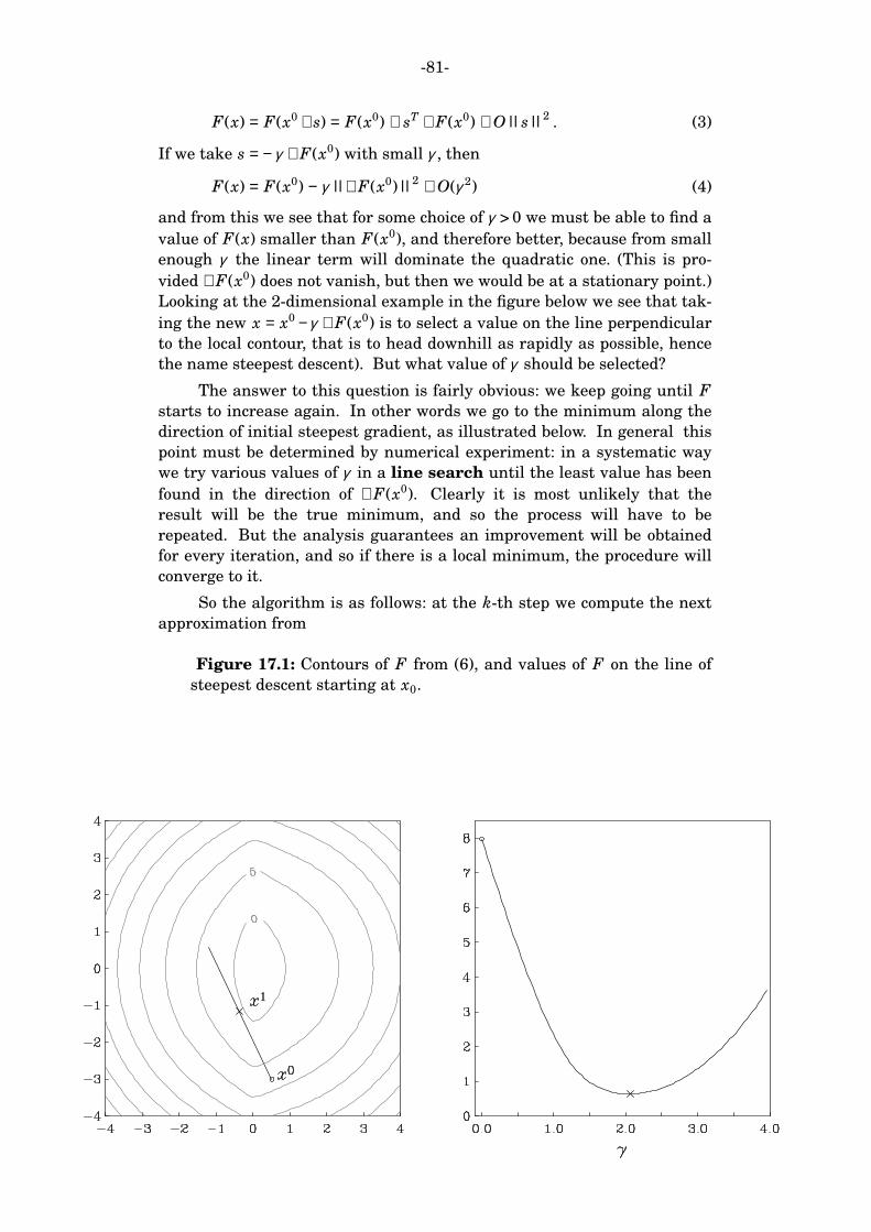
-81-
F(x) = F(x0 + s) = F(x0) + sT ∇ F(x0) + O||s||2
. (3)
If we take s = −γ ∇ F(x0) with small γ , then
F(x) = F(x0) − γ ||∇ F(x0)||2 + O(γ 2) (4)
and from this we see that for some choice of γ > 0 we must be able to find a
value of F(x) smaller than F(x0), and therefore better, because from small
enough γ the linear term will dominate the quadratic one. (This is pro-
vided ∇ F(x0) does not vanish, but then we would be at a stationary point.)
Looking at the 2-dimensional example in the figure below we see that tak-
ing the new x = x0 −γ ∇ F(x0) is to select a value on the line perpendicular
to the local contour, that is to head downhill as rapidly as possible, hence
the name steepest descent). But what value of γ should be selected?
The answer to this question is fairly obvious: we keep going until F
starts to increase again. In other words we go to the minimum along the
direction of initial steepest gradient, as illustrated below. In general this
point must be determined by numerical experiment: in a systematic way
we try various values of γ in a line search until the least value has been
found in the direction of ∇ F(x0). Clearly it is most unlikely that the
result will be the true minimum, and so the process will have to be
repeated. But the analysis guarantees an improvement will be obtained
for every iteration, and so if there is a local minimum, the procedure will
converge to it.
So the algorithm is as follows: at the k-th step we compute the next
approximation from
Figure 17.1: Contours of F from (6), and values of F on the line of
steepest descent starting at x0.
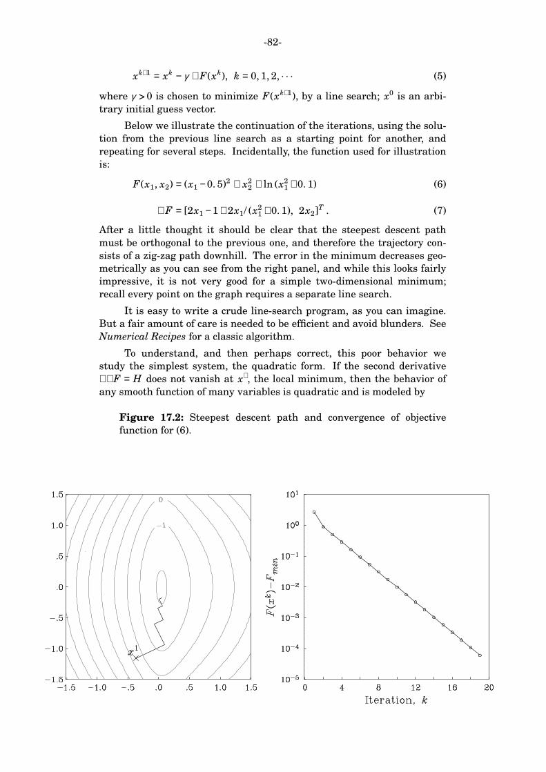
-82-
xk+1 = xk − γ ∇ F(xk), k = 0, 1, 2, . . . (5)
where γ > 0 is chosen to minimize F(xk+1), by a line search; x0 is an arbi-
trary initial guess vector.
Below we illustrate the continuation of the iterations, using the solu-
tion from the previous line search as a starting point for another, and
repeating for several steps. Incidentally, the function used for illustration
is:
F(x1, x2) = (x1 −0. 5)2 + x22 + ln (x2
1 +0. 1) (6)
∇ F = [2x1 −1 + 2x1/ (x21 +0. 1), 2x2]T . (7)
After a little thought it should be clear that the steepest descent path
must be orthogonal to the previous one, and therefore the trajectory con-
sists of a zig-zag path downhill. The error in the minimum decreases geo-
metrically as you can see from the right panel, and while this looks fairly
impressive, it is not very good for a simple two-dimensional minimum;
recall every point on the graph requires a separate line search.
It is easy to write a crude line-search program, as you can imagine.
But a fair amount of care is needed to be efficient and avoid blunders. See
Numerical Recipes for a classic algorithm.
To understand, and then perhaps correct, this poor behavior we
study the simplest system, the quadratic form. If the second derivative
∇∇ F = H does not vanish at x∗ , the local minimum, then the behavior of
any smooth function of many variables is quadratic and is modeled by
Figure 17.2: Steepest descent path and convergence of objective
function for (6).
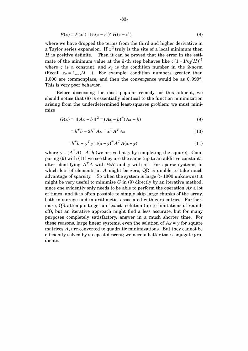
-83-
F(x) = F(x∗ ) + ½(x − x∗ )T H(x − x∗ ) (8)
where we have dropped the terms from the third and higher derivative in
a Taylor series expansion. If x∗ truly is the site of a local minimum then
H is positive definite. Then it can be proved that the error in the esti-
mate of the minimum value at the k-th step behaves like c [1 − 1/κ 2(H)]k
where c is a constant, and κ 2 is the condition number in the 2-norm
(Recall κ 2 = λ max/λ min). For example, condition numbers greater than
1,000 are commonplace, and then the convergence would be as 0. 999k.
This is very poor behavior.
Before discussing the most popular remedy for this ailment, we
should notice that (8) is essentially identical to the function minimization
arising from the underdetermined least-squares problem: we must mini-
mize
G(x) = ||Ax − b||2 = (Ax − b)T (Ax − b) (9)
= bT b − 2bT Ax + xT AT Ax (10)
= bT b − yT y + (x − y)T AT A(x − y) (11)
where y = (AT A)−1 AT b (we arrived at y by completing the square). Com-
paring (9) with (11) we see they are the same (up to an additive constant),
after identifying AT A with ½H and y with x∗ . For sparse systems, in
which lots of elements in A might be zero, QR is unable to take much
advantage of sparsity. So when the system is large (> 1000 unknowns) it
might be very useful to minimize G in (9) directly by an iterative method,
since one evidently only needs to be able to perform the operation Ax a lot
of times, and it is often possible to simply skip large chunks of the array,
both in storage and in arithmetic, associated with zero entries. Further-
more, QR attempts to get an "exact" solution (up to limitations of round-
off), but an iterative approach might find a less accurate, but for many
purposes completely satisfactory, answer in a much shorter time. For
these reasons, large linear systems, even the solution of Ax = y for square
matrices A, are converted to quadratic minimizations. But they cannot be
efficiently solved by steepest descent; we need a better tool: conjugate gra-
dients.
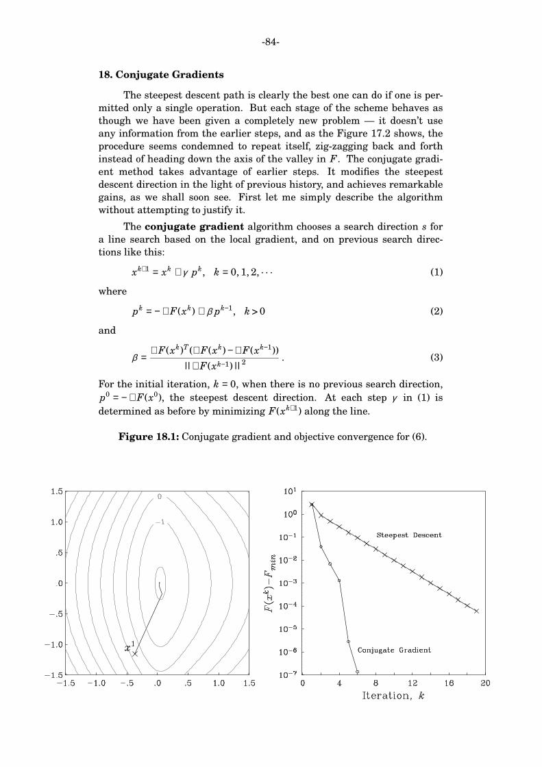
-84-
18. Conjugate Gradients
The steepest descent path is clearly the best one can do if one is per-
mitted only a single operation. But each stage of the scheme behaves as
though we have been given a completely new problem — it doesn’t use
any information from the earlier steps, and as the Figure 17.2 shows, the
procedure seems condemned to repeat itself, zig-zagging back and forth
instead of heading down the axis of the valley in F. The conjugate gradi-
ent method takes advantage of earlier steps. It modifies the steepest
descent direction in the light of previous history, and achieves remarkable
gains, as we shall soon see. First let me simply describe the algorithm
without attempting to justify it.
The conjugate gradient algorithm chooses a search direction s for
a line search based on the local gradient, and on previous search direc-
tions like this:
xk+1 = xk + γ pk, k = 0, 1, 2, . . . (1)
where
pk = − ∇ F(xk) + β pk−1, k > 0 (2)
and
β =∇ F(xk)T (∇ F(xk) − ∇ F(xk−1))
||∇ F(xk−1)||2
. (3)
For the initial iteration, k = 0, when there is no previous search direction,
p0 = − ∇ F(x0), the steepest descent direction. At each step γ in (1) is
determined as before by minimizing F(xk+1) along the line.
Figure 18.1: Conjugate gradient and objective convergence for (6).

-85-
On the prevous page we show the results of the application to the
minimization of (5). The improvement on steepest descent is extraordi-
nary, as the right panel shows. Notice also that the convergence is not a
steady exponential decline in error; the rate varies. This is a feature of
conjugate gradient optimization: it may chug along reducing the penalty
only modestly, then make a huge gain, then settle back to slower progress.
Such behavior makes a termination strategy difficult to devise, because
one cannot tell when the penalty has been reduced to its minimum value.
Remember, the convergence plots in these notes are cheats, because I
know the real answer, something obviously not normally available.
The design of the conjugate gradient method is centered on the goal
of solving a problem with a quadratic penalty function, like (8), exactly
after precisely n iterative steps, where n is the dimension of the space of
unknowns. When solving a very large system (with n > 1000, say), one
would not want to have to take so many steps, but it is often the case that
an exact answer is not required, and a perfectly satisfactory reduction in
the penalty function will have been achieved long before k = n. It also
turns out that for very large systems, exact answers cannot be obtained in
practice even after n iterations, because of the accumulation of round-off
error in the computer arithmetic.
Here is an explanation of how conjugate gradients work, taken from
Gill et al., Chap 4. Strang, and Golub and Van Loan, offer different
derivations which are longer. As just remarked the procedure is set up to
solve a quadratic problem, which we will take to be the minimization of
F(x) = c ⋅ x + ½x ⋅ Gx (4)
where G ∈ IRn×n and is positive definite and symmetric. For this last
proof we will use the familiar notation x ⋅ y to be the inner product of two
vectors because it is much cleaner: so recall x ⋅ y = xT y = yT x. Also, since
G is symmetric, note that x ⋅ Gy = y ⋅ Gx.
The exact minimum of F is easily seen to be the point x∗ = − G−1c, so
solution of (4) by conjugate gradients is equivalent to solving that linear
system of equations. You will easily verify that
∇ F(x) = c + Gx . (5)
We look at the process at iterative step k; we assume we have an approxi-
mation for the minimizer xk and we are going build the next approxima-
tion by a linear combination of vectors, p0, p1, . . . pk collected over previ-
ous iterations, together with the current approximation to the solution;
we will explain later how the vectors pk are chosen. For now we assert:
xk+1 = xk +k
j=0Σ w j p j (6)
= xk + Pkw (7)
-86-
where the matrix P = [ p0, p1, . . . pk] and the vector w contains the
weights. Our first job is to find w so that xk+1 in (7) minimizes F. This is
a straightforward least-squares problem, details omitted. We find
w = − (PTk GPk)−1 PT
k gk (8)
where the vector gk is defined as the gradient:
gk = ∇ F(xk) = c + Gxk . (9)
Plugging (8) into (7) gives
xk+1 = xk − Pk(PTk GPk)−1 PT
k gk . (10)
At this point we note a useful property of the process: the gradient at the
k + 1-st approximation is orthogonal to all the current vectors pi. Proof —
calculate:
PTk gk+1 = PT
k ∇ F(xk+1) = PTk (c + Gxk+1) (11)
= PTk (gk − Gxk + G(xk − Pk(PT
k GPk)−1 PTk gk)) (12)
= PTk gk − PT
k GPk(PTk GPk)−1 PT
k gk (13)
= 0. (14)
By expanding Pk into column vectors we see this means:
PTk gk+1 = [ p0 ⋅ gk+1, p1 ⋅ gk+1, . . . pk ⋅ gk+1]T = [0, 0, . . . 0]T (15)
and therefore
pi ⋅ gk+1 = gk+1 ⋅ pi = 0, i = 0, 1, 2, . . . k . (16)
Now if we assert that all the xk to this point have been found in the same
wa y, it must be true that for j = 1, 2, . . . k
pi ⋅ g j = g j ⋅ pi = 0, i < j . (17)
Thus the gradient vector g j is orthogonal to every earlier pi vector, as
advertised.
With this information let us calculate the product PTk gk at the end of
(10):
PTk gk = [ p0 ⋅ gk, p1 ⋅ gk, . . . pk ⋅ gk]T = [0, 0, . . . 0, α ]T (18)
where α = pk ⋅ gk.
So far the only property assumed of the pi has been linear indepen-
dence, needed for the inverse in (8). Let us now assert that we would like
another property (which we will have to build into process somehow): let
us propose that the vectors pi are mutually conjugate under the action
of G. This means that they orthogonal in the G inner product, or explic-
itly that

-87-
( pi, p j)G = pi ⋅ Gp j = 0, i ≠ j . (19)
Then the matrix PTk GPk in (10) becomes a diagonal matrix. Combining
that fact with (18), which is always true, the expression xk+1 in (10) sim-
plifies to
xk+1 = xk + γk pk (20)
which is (1). In other words, when we started, the search for the mini-
mum at step k was over the complete set of previous vectors p j , but with
conjugacy we find only the most recent vector need be searched over to
achieve the optimal result. The parameter γk which we happen to know is
γk = −α
pk ⋅ Gpk= −
pk ⋅ gk
pk ⋅ Gpk(21)
could be found by a line search, and would have to be if this were a lin-
earization of a nonquadratic system.
To summarize: if we can somehow arrange the vectors pi to be
mutually conjugate, they are the search directions at each iterative step,
and at the end of that step, F has achieved its minimum over the space
spanned by the vectors p0, p1, . . . pk. Since these vectors are linearly
independent and at step n −1 there are n of them, they must span IRn,
and therefore at this last step we must have the global minimum of F
over all vectors in IRn. Our task is to set up a scheme for producing
search direction vectors pi with the property of conjugacy under G.
We set about building the pi from the available gradients as follows.
First we take p0 = − g0 (the steepest descent direction; why?). Subse-
quently we say
pk = − gk +k−1
j=0Σ β kj p j (22)
that is, the new direction is found from the current gradient and a linear
combination of previous search directions. In what follows we work
towards determining the values of the unknown coefficients β kj in this
expansion. By a simple rearrangement, it follows from the recipe (22)
that gk is a linear combination of the p j up to j = k: Consider i < k and
dot a gradient vector with any earlier gradient vector:
gk ⋅ gi = gk ⋅i
j=0Σ σ j p j =
i
j=0Σ σ j gk ⋅ p j (23)
= 0 (24)
because of (17). So the gradient vectors are mutually orthogonal too!
To discover the coefficients β kj we make use of the mutual conjugacy
of the pi vectors — we pre-multiply (22) by G, then dot on the left with pi:

-88-
pi ⋅ Gpk = − pi ⋅ Ggk +k−1
j=0Σ β kj pi ⋅ Gp j . (25)
Then for i < k, because of the conjugacy, (19), the left side vanishes and so
do most of the terms in the sum:
0 = − pi ⋅ Ggk + β ki pi ⋅ Gpi, i < k (26)
= − gk ⋅ Gpi + β ki pi ⋅ Gpi . (27)
From (9), the definition of gi, and using (20) we see
gi+1 − gi = G(xi+1 − xi) = γiGpi . (28)
This allows us to substitute for Gpi in (27):
0 = −1
γi
gk ⋅ (gi+1 − gi) + β ki pi ⋅ Gpi . (29)
But now the orthogonality of the gradients, (24), means that when i < k −1
the first term on the right automatically vanishes too; since pi ⋅ Gpi must
not be zero,
β ki = 0, i < k −1 . (30)
Hence we have just shown that to get conjugacy of search directions, the
new search direction at each step involves the current gradient and the
previous direction only; (22) has become:
pk = − gk + β k,k−1 pk−1 (31)
which is of course (2). Finally we need to find the coefficient β k,k−1 explic-
itly. Premultiply (31) by G then dot with pk−1; conjugacy makes pk−1 ⋅ Gpk
on the left side vanish, and so, rearranging we find
β k,k−1 =pk−1 ⋅ Ggk
pk−1 ⋅ Gpk−1(32)
=(gk − gk−1) ⋅ gk
gk−1 ⋅ gk−1(33)
=gk ⋅ gk
gk−1 ⋅ gk−1=
||gk||2
||gk−1||2
(34)
where (33), (34) follow from applications of (16), (24) and (28). The form
(33) is used in the nonquadratic application (3) rather than (34) because
when the problem is not quadratic, orthogonality of the successive gradi-
ents is only approximate.
Powerful as CG certainly is, it still may require a lot of numerical
work when the dimension of the system becomes very large. Then there a
further tricks that can improve the convergence rate, but they are depen-
dent on special structure a particular problem may exhibit, and are not
-89-
generally available. The concept is called preconditioning, and is cov-
ered in Golub and Van Loan, Chapter 10.
Bibliography
Gill, P. E., Murray, W. and Wright, M. H., Practical Optimization, Aca-
demic Press, New York, 1981.
A treasure trove of numerical methods for every kind of optimization
problem: linear, nonlinear, constrained, unconstrained, sparse, full, linear
programming.
Golub, G., and Van Loan , C., Matrix Computations, 3rd Edition, Johns
Hopkins Univ. Press, 1996.
The one reference for matrix linear algebra.
Lawson, C. L., and Hanson, R. J. , Solving Least Squares Problems, 1974.
Classic text for full analysis of QR and SVD in least squares.
Strang, G., Introduction to Applied Mathematics, Wellesley-Cambridge,
1986.
Readable treatment of many topics, though sometimes a little off base.
-90-
19. Application to the Gravity Anomaly Problem
The nonlinear gravity inversion problem in GIT was solved there by
means of Occam and by B-G creeping. As a finale we will apply steepest
descents and conjugate gradients to it. We have already computed (in
GIT) the Frechet Derivative for the problem, but as I want to stress here,
those derivatives do not all need to be stored, or a Gram matrix inverted
for SD or CG. This makes them more suitable for very large problems,
which the gravity problem is not, of course.
First we need a scalar function to minimize. This immediately
points up one of the disadvantages of these optimization methods: they
are designed for unconstrained optimization. If we are seeking a regular-
ized solution we will need to minimize something like
U (h, λ ) =N
j=1Σ (d j − F j[h])2 + λ ||h||
2(1)
where λ is the unknown Lagrange multiplier whose value we discover by
achieving the appropriate misfit. In nonlinear problems, however, the
first order of business is to get any solution at all, and so initially we
might choose λ to be very small, or zero. In case of the gravity problem
we first want to fit the data almost exactly, and since the topography is
order of magnitude unity, setting λ = 0. 01 will insure most emphasis is
placed on the first term. The derivative of U is just a vector in the dis-
cretized form: ∇ U ∈ IRL, where L = the number sample points in h(x);
while the Frechet derivative is approximated by the matrix D ∈ IRN×L.
We easily calculate that
∇ U = 2DT (d − F) + 2λ h (2)
where d − F ∈ IRN is the vector of misfits. We should not forget to note
that:
d j = F j[h] =G∆ρa
0
∫ ln
(x − x j)2 + h(x)2
(x − x j)2
dx (3)
D j(x) =2G∆ρ h(x)
(x − x j)2 + h(x)2
(4)
The discretized form of (3) and (4) follows easily by replacing the function
h(x) with the vector of samples [h1, h2, . . . hL]. In the calculations that fol-
low we take L = 50.
First we perform the minimization using steepest descent steps,
starting at the model that is a constant h(x) = 1 km; λ = 0. 01. The
squared norm of misfits is shown in Figure 19.1, plotted against step
number: each step involves the line search along the steepest descent
direction. At the end of 50 line searches the penalty function U in (1) was
reduced to 0. 327 mGal2 and the norm of misfits was 0.391 mGal. Next we
perform the conjugate gradient minimization, starting at the same initial

-91-
Figure 19.1: Penalty function U after n line searches with (+) steep-
est descents; (o) conjugate gradients.
guess. This is shown in the Figure too. Notice how the initial perfor-
mance is worse than steepest descents, but then the method beats steep-
est descents: after 50 steps we have a penalty of 0. 272 mGal2 and a misfit
2-norm of 0.300 mGal. The models are shown on the next page in Figure
19.2.
At first glance these methods appear to be at a severe disadvantage
to Occam, which needed only four line searches to reach a similar misfit
level. But that is not necessarily the case, as we now discuss. Each line
search in Occam requires the solution of the linear system of equations
1
µI + D DT
α = d (5)
(This is (25) on p 315 of GIT.) This uses on the order of N3 computer oper-
ations, since D DT ∈ IRN . Whereas the single line search in SD or CG
involves nothing more than operations of addition and subtraction of vec-
tors, for which the computer costs are only order N . In fact, the largest
cost in each step is the evaluation of ∇ U , which here takes order N2 oper-
ations. For large data sets CG (or SD) have a much lower cost per step.
In this light, the cost for 50 steps of CG is about the same as 4 steps of
Occam, since N = 12. So when N is very large, say hundreds or even
thousands, CG may be the only practical approach.
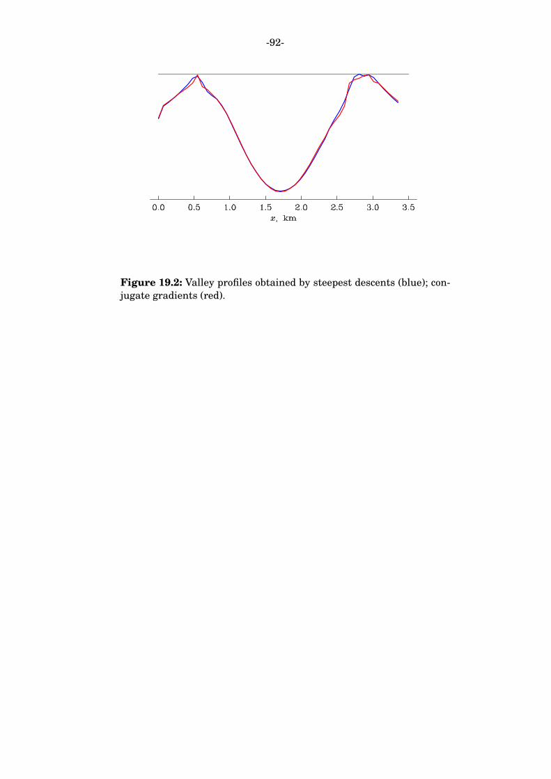
-92-
Figure 19.2: Valley profiles obtained by steepest descents (blue); con-
jugate gradients (red).