SINGLE-WELL TRACER PUSH-PULL METHOD

DEVELOPMENT FOR SUBSURFACE PROCESS

CHARACTERIZATION

Early-time tracer injection-flowback test for stimulated fracture

characterization, numerical simulation uses and efficiency for flow and

solute transport

Dissertation

-to acquire the doctoral degree in mathematics and natural science

"Doctor rerum naturalium"

-at the Georg-August-Universität Göttingen

in the doctoral program Geoscience

at Georg-August University School of Science (GAUSS)

Submitted by

Shyamal Karmakar

from Rangamati, Bangladesh

Göttingen, 2016

ii

Betreuungsausschuss:

Professor Dr. Martin Sauter, GZG – Abteilung Angewandte Geologie, Universität Göttingen

Dr. Iulia Ghergut, GZG – Abteilung Angewandte Geologie, Universität Göttingen

Mitglieder der Prüfungskommission

Referent:

Professor Dr. Martin Sauter, GZG – Abteilung Angewandte Geologie, Universität Göttingen

Koreferent:

Dr. Iulia Ghergut, GZG – Abteilung Angewandte Geologie, Universität Göttingen

Professor Dr. Günter Buntebarth, Instituts für Geophysik, Technische Universität Clausthal

weitere Mitglieder der Prüfungskommission:

Professor Dr.-Ing. Thomas Ptak-Fix, GZG – Abteilung Angewandte Geologie, Universität

Göttingen

Dr. Reinhard Jung, Jung Geotherm, Isernhagen, Hannover

Dr. Ulrich Maier, GZG – Abteilung Angewandte Geologie, Universität Göttingen

Tag der mündlichen Prüfung: 15.06.2016

iii

To my Mother

and to my TEACHERS

iv

Summary

Geological inherent knowledge, hydraulic test and geophysical methods can estimate most of the

stimulated georeservoir properties. The transport effective parameters such as fracture aperture

and effective porosity cannot estimate by using these methods. The in-situ methods, the inter-well

test or single-well test, are sensitive to transport effective parameters. Transport effective

parameters determine geo reservoir's efficiency, sustainability or lifetime. The inter-well test

needs more than one well which is not typical to install during early stage of geo-reservoir

development to avoid too much investment before a proven use is confirmed. Hence, single-well

test design for a specific sensitivity regime from ‘early’ to ‘very-late’ pull signal is rather practical

for transport effective parameter estimation. Moreover, a typical single-well test that design for

‘mid’ to ‘late-time’ signal also loaded with many sensitive parameters. Secondly, tracer test

design, and parameter sensitivity estimation depends on numerical simulation reliability. Finite

element and finite difference code based different numerical method shows significant

improvement toward this parameter inversion and test design.

The use of single-well (SW) short-term tracer signals to characterize stimulated fractures at the

Groß-Schönebeck EGS pilot site is studied in chapter 2, part 1. Short-time tracer flowback signals

suffer from ambiguity in fracture parameter inversion from measured single-tracer signals. This

ambiguity arises commonly due to a certain degree of interdependence between parameters such

as fracture porosity, fracture thickness, fracture dispersivity. This ambiguity can, to some extent,

be overcome by (a) combining different sources of information, and/or (b) using different types

of tracers, such as conservative tracer pairs with different diffusivities, or tracer pairs with

contrasting sorptivity on target surfaces. Fracture height is likely to be controlled by

lithostratigraphy while fracture length can be determined from hydraulic monitoring (pressure

signals). Since the flowback rate is known during an individual-fracture test, the unknown

parameters to be inferred from tracer tests are (i) transport-effective aperture in a water fracture

or (ii) fracture thickness and porosity for a gel-proppant fracture. Tracers with different sorptivity

on proppant coatings and matrix rock surfaces for gel-proppant fractures and tracers with

contrasting-diffusivity or -sorptivity for a water fracture were considered. This simulation study

has produced two significant results: (1) water fracture aperture can be effectively evaluated based

on early-time tracer signals of a conservative tracer; and (2) by using the combination of matrix

sorptive and proppant sorptive tracers, it is possible to estimate fracture thickness and porosity in

gel proppant fractures from a single test. The injection and flowback of a small fluid volume, and

thus little dilution of the injected tracers, has three practical advantages: (1) there is no need to

v

inject large tracer quantities; (2) one does not have to wait for the tails of the test signals; and (3)

the field and laboratory monitoring of the tracer signals does not have to be conducted for ultra-

low tracer concentrations, which is known to be a major challenge, with the highly-mineralized

and especially high organic content fluids typically encountered in many sedimentary basement

georeservoir. Additionally, it requires only a very small chaser injection volume (about half of

fracture volume).

Short-term flowback signals from injection-flowback tracer test face a certain degree of ambiguity

in fracture parameter inversion from the measured signal of a single tracer. To improve the early-

time characterization of induced fractures, of either gel-proppant or waterfrac, we recommend

using tracers of contrasting sorptivity to rock surfaces, and to proppant coatings where applicable.

The application that described in early time flowback tracer test study article at chapter 2, part 1.

However, the tracer was not exhaustively demonstrating its complete range of uses for stimulated

georeservoir. Sorptive tracer either on proppant or on a matrix that used for stimulated fracture

characterization has raised the question about the range of sorptive tracer to produce for an

effective tracer test. For the purposes, a lower sorptive tracer than its minimum necessary was

suggested and a sensitivity improvement factor (ratio between sorptive tracer signal changes to

conservative tracer signals changes, s/c) approximately equal to √ (1 + 0.7× sorption coefficient,

κ) is formulated. One needs to note that the higher the tracer's retardation, the lower is its fracture

invasion, and consequently a poorer capability for characterizing the fracture as a whole. In

principle, this could be compensated by increasing the chaser volume (i.e., by injecting sorptive

tracers earlier than conservative tracers).

Modeling flow and solute transport become a state of the art for a set of engineering and

hydrogeological applications. For hydrogeological modeling, a number of numerical software is

available as commercial code as well as many research initiatives is emerging to develop a new

one. This section (Chapter 3) of the thesis attempts to develop solute transport module in fracture

using COMSOL. FEFLOW software with it discrete feature element (e.g. fracture) module it can

simulate fully couple process for flow, solute, and heat simulation. For the study of early time,

tracer flowback signal, the flow, and solute transport process coupling in fracture-matrix domain

is studied using tetrahedral mesh. To compare the consistency of numerical result with spatial and

temporal discretization as well as in different numerical approach, a same numerical model set

up in COMSOL. Qualitative comparison of the between the codes reveals that dispersivity tensor

application can cause a minor variation in the tracer breakthrough in single-well tracer flowback

vi

simulation. The result is compared in terms similarities and capturing the spikes of injection and

flowback in early flow back tracer test.

A set of well-established software, frequently used for modeling flow and transport in geological

reservoirs, is tested and compared (MODFLOW/MT3DMS, FEFLOW, COMSOL Multiphysics

and DuMux). Those modeling tools are based on different numerical discretization schemes i.e.

finite differences, finite volumes and finite element methods. The influence of dispersivity, which

is directly related to the numerical modeling, is investigated in parametric studies and results are

compared with analytical approximations. At the same time, relative errors are studied in a

complex field scale example. For 1D and 2D cases all three tested modeling software show good

agreement with the analytical solutions. By refining the grid discretization all four software

packages get an improvement in accuracy. It is shown for the 2D problem that COMSOL

Multiphysics needs a finer mesh to produce the same accuracy as FEFLOW and DuMux. For

transport simulations in forced gradient, where a commonly expected dispersion or higher value

occurs, the finite element software FEFLOW is the best choice. From this comparative study, it

is revealed that under forced gradient conditions, finite element codes COMSOL and FEFLOW

show a higher accuracy with respect to the analytical approximation for a certain range of

dispersivity than DuMux and MODFLOW/MT3DMS. Comparing simulation time and code

parallelization, FEFLOW performs better than COMSOL. Computational time is lowest for finite

difference software MODFLOW/MT3DMS for a small number of mesh elements (~ less than

12800 elements). For large meshes (12800 elements or higher) finite element software FEFLOW

performs better. Nevertheless, the study showed that improving the numerical performance by

optimizing discretization methods, solvers and parallelization methods still remain a crucial field

of research.

vii

Table of Contents

Single-well tracer push-pull method development for subsurface process characterization

..................................................................................................................................................... i

Table of Contents ................................................................................................................... vii

List of Figures .......................................................................................................................... xi

List of Tables.......................................................................................................................... xiv

CHAPTER 1: INTRODUCTION .................................................................................................. 1

1 Introduction ............................................................................................................................ 2

1.1 Renewable energy sources and geothermal energy......................................................... 2

1.2 Significance of fracture characterization for stimulated geo-reservoir ........................... 2

1.3 Single well tracer test and tracer flowback for fracture characterization ........................ 3

1.4 Early time tracer signal ................................................................................................... 4

2 Objectives of this thesis .......................................................................................................... 6

2.1 Single well tracer push-pull/injection-flowback test: dispersion in porous media and

fractured porous media; Chapter 2- Part 1, Part 2 and Part 3..................................................... 7

2.1.1 Part 1: Early-time tracer signal for fracture thickness, fracture porosity, and

dispersivity in gel-proppant fracture and dispersivity, fracture aperture in water fracture .... 8

2.1.2 Part 2: Early time tracer injection-flowback test: injection duration- ‘Tpush’ and

‘injection rate’ effect on the parameter sensitivity ................................................................. 8

2.1.3 Part 3: Multiple fracture and single fracture systems for sorption-matrix diffusion

based model ............................................................................................................................ 8

2.2 Benchmark study on flow and solute transport; Chapter 3- Part 1 and Part 2 ................ 9

2.2.1 Part 1: Spatial and temporal discretization sensitivity to single fracture simulation

using finite element code FEFLOW and COMSOL- a benchmark study .............................. 9

2.2.2 Part 2: Benchmark Study On Flow and Solute Transport in Geological

Reservoirs ............................................................................................................................... 9

References .................................................................................................................................... 10

CHAPTER 2-PART 1: Early-flowback tracer signals for fracture characterization in an EGS

developed in deep crystalline and sedimentary formations: a parametric study ......................... 14

Abstract ........................................................................................................................................ 15

1 Introduction .......................................................................................................................... 16

2 Gel-proppant fracturing (GPF) and water fracturing (WF) .................................................. 17

3 Model setup, transport processes, and simulation parameters for tracer tests ...................... 18

4 Spatial discretization and hydraulic treatment of injection-flowback tests .......................... 22

5 Parameter interplay, and numerical simulations ................................................................... 24

6 Results .................................................................................................................................. 26

6.1 Conservative-tracer signals during early flowback ....................................................... 26

viii

6.2 MST signals during early flowback .............................................................................. 29

6.3 PST signals during early flowback in GPF fractures .................................................... 32

7 Discussion, and recommendations for future tracer tests ..................................................... 34

References .................................................................................................................................... 37

CHAPTER 2-PART 2: EGS in sedimentary basins: sensitivity of early-flowback tracer signals to

induced fracture parameters ......................................................................................................... 40

Abstract ........................................................................................................................................ 41

1 Introduction .......................................................................................................................... 42

2 Gel proppant fracture and water fracture simulation parameters ......................................... 43

3 Conservative and sorptive tracer test in gel proppant fracture ............................................. 43

1.1 Conservative tracer ........................................................................................................ 43

1.2 Matrix sorptive tracer .................................................................................................... 45

1.3 Proppant sorptive tracer ................................................................................................ 46

2 Conservative and sorptive tracer test in water fracture ........................................................ 48

2.1 Conservative tracer ........................................................................................................ 48

3 Summary and conclusions .................................................................................................... 49

References .................................................................................................................................... 50

CHAPTER 2-PART 3: Early time flowback tracer test for stimulated crystalline-georeservoir of

multiple parallel fracture characterization ................................................................................... 51

Abstract ........................................................................................................................................ 52

1 Introduction .......................................................................................................................... 53

2 Model concept and parameter selection ............................................................................... 54

2.1 Fracture model for injection-flowback test ................................................................... 55

3 Results .................................................................................................................................. 56

4 Sorption tracer selection and sensitivity ............................................................................... 60

5 Discussion and conclusion.................................................................................................... 63

References .................................................................................................................................... 65

CHAPTER 3-PART 1: Single-well tracer injection-flowback test simulation in fractured

georeservoir using finite element code FEFLOW and COMSOL- a benchmark study .............. 66

Abstract ........................................................................................................................................ 67

1 Model concept ...................................................................................................................... 67

2 Results and Discussion ......................................................................................................... 71

2.1 Spatial and Temporal discretization effect on FEFLOW single fracture SW injection

flowback tracer breakthrough................................................................................................... 71

2.2 Tracer flowback signals in COMSOL and FEFLOW from gel-proppant fracture and

water fracture, simulation concept and limitation .................................................................... 73

ix

References .................................................................................................................................... 75

CHAPTER 3-Part 2: A set of benchmark studies on flow and solute transport in geological

reservoirs ...................................................................................................................................... 76

Abstract ........................................................................................................................................ 77

1 Introduction .......................................................................................................................... 77

2 Methodology ......................................................................................................................... 79

2.1 Mathematical model ...................................................................................................... 79

2.2 Problem definition ......................................................................................................... 80

2.2.1 Problem 1: 1D - Solute tracer transport for steady state flow with a forced head

gradient in a homogenous aquifer ........................................................................................ 81

2.2.2 Problem 2: 2D-Solute transport in a confined homogenous aquifer from a forced

gradient point source ............................................................................................................ 81

2.2.3 Problem 3: 3D- Solute transport for confined homogeneous multi-layered forced

gradient conditions ............................................................................................................... 82

3 Benchmarking simulators ..................................................................................................... 83

3.1 MODFLOW/MT3DMS: ............................................................................................... 84

3.2 FEFLOW 6.0: ................................................................................................................ 84

3.3 COMSOL Multiphysics 4.4 .......................................................................................... 85

3.4 DuMux ........................................................................................................................... 86

4 Result .................................................................................................................................... 86

4.1 Problem 1: 1D – Solute transport in a homogeneous aquifer with a natural gradient .. 86

4.2 Problem 2: 2D-Solute transport in forced gradient homogeneous aquifer.................... 88

4.2.1 Spatial discretization effects on solution efficiency .............................................. 89

4.3 Problem 3: 3D -Flow and solute transport simulation in a layered georeservoir .......... 90

4.4 Simulation time (CPU time) of single processor and parallelization ............................ 94

5 Discussion ............................................................................................................................. 96

5.1 User friendliness ............................................................................................................ 96

5.2 Solute transport simulation efficiency of the benchmark problems .............................. 97

5.3 Model implementation, simulation time and resource use efficiency and discretization .

....................................................................................................................................... 99

6 Conclusions ........................................................................................................................ 100

References .................................................................................................................................. 101

CHAPTER 4: GENERAL DISCUSSION, CONCLUSIONS, AND FUTURE WORK........... 103

1 Discussion and conclusion.................................................................................................. 104

1.1 Single well tracer injection-flowback/withdrawal test-early-time tracer signal study 104

1.2 Tracer selection for early time tracer injection-flowback test..................................... 107

1.3 Benchmark study for efficient numerical method selection and code development ... 108

x

2 A way forward .................................................................................................................... 109

2.1 Early time solute tracer push-pull test for dispersion estimation in aquifer................ 109

2.2 Heat tracer uses for pulse injection flowback test-design and parameter estimation .. 110

2.3 Solute tracer pulses injection flowback test-design and parameter estimation in shale/gas

reservoir characterization ....................................................................................................... 111

3 Final remark ........................................................................................................................ 113

References .................................................................................................................................. 114

Appendix 1-Early flowback tracer signal for fracture characterization using proppant sorptive,

matrix sorptive and conservative tracers.................................................................................... 117

Appendix 2a: Single-well tracer injection-flowback test simulation in fractured georeservoir in

FEFLOW and COMSOL ........................................................................................................... 119

Appendix 2b: A set of benchmark studies for flow and solute transport in geo-reservoir ........ 121

List of Publications .................................................................................................................... 127

Conference proceedings, poster, and oral presentation ............................................................. 127

Curriculum Vitae ....................................................................................................................... 129

Acknowledgement ..................................................................................................................... 130

xi

List of Figures

Figure 2.3.1: 3D model domain and hydrogeological parameter distribution (after Blöcher et al., 2010)

.................................................................................................................................................................. 20

Figure 2.4.1: Fluid and tracer injection-flowback in GPF and WF treatments. The transition from constant

injection to constant flowback was approximated as linear (dashed-line segment); its duration is enlarged

for better recognition. In the simulations, the transition spans only 1/60 of Tpush. .............................. 23

Figure 2.6.1: Simulated signals of conservative tracers during GPF flowback: the effect of dispersion

processes (expressed by eight different values of longitudinal dispersivity αL, as indicated by signal labels,

in meters), shown for two different values of GPF thickness (solid line: 12mm, dashed-dotted line: 20mm),

with a fixed value of GPF porosity (45%). ................................................................................................. 27

Figure 2.6.2: Simulated signals of conservative tracers during GPF flowback: the effect of dispersion

processes (expressed by eight different values of longitudinal dispersivity αL, as indicated by signal labels,

in meters), shown for three different values of GPF porosity (solid line: 30%, dashed line: 45%, dashed-

dotted line: 60%), with a fixed value of GPF thickness (12mm). ............................................................... 28

Figure 2.6.3: Simulated signals of conservative tracers during WF flowback: the distinct effects of fracture

aperture (with values represented by different shadings as shown by legend) and of longitudinal

dispersivity (solid line: 7m, dash-dotted line: 5m). ................................................................................... 29

Figure 2.6.4: Simulated signals of various MST (characterized by different Kd values) during GPF flowback,

at a fixed value of GPF thickness (12mm) and proppant-packing porosity 30%). Signals are labeled by the

retardation factor R, instead of Kd values the signal of a conservative (non-sorptive, Kd=0, R=1) tracer is

shown for comparison. .............................................................................................................................. 30

Figure 2.6.5: Simulated signals of two MST during GPF flowback: the effect of GPF thickness (values are

indicated as signal labels, in mm), with a fixed value of proppant-packing porosity (45%), shown for two

tracer species, a less sorptive one (dimensionless 𝜅= 0.9), and a more sorptive one (dimensionless 𝜅=1.52).

.................................................................................................................................................................. 31

Figure 2.6.6: Simulated signals for one MST (characterized by dimensionless κ= 1.5) during GPF flowback:

the effect of GPF thickness (values are indicated as signal labels, in mm), with two values of GPF porosity

(solid line: 30%, broken line: 60%) ............................................................................................................ 32

Figure 2.6.7: Simulated signals for one PST (characterized by dimensionless κ=40) during GPF flowback:

the effects of GPF thickness and of GPF porosity (solid lines: 35%, broken lines: 55%) illustrate parameter

interplay. ................................................................................................................................................... 33

Figure 2.6.8: Simulated signals for one PST (characterized by dimensionless κ =40) during GPF flowback:

the effect of GPF thickness (values are indicated in mm), and the effect of GPF porosity (gray tones, from

light: 30%, to dark: 60%), illustrating the increase of porosity sensitivity with increasing thickness. ...... 34

Figure 2.2.1: Conservative tracer flowback signals from different dispersivity and fracture thickness:

broken line- 4mm, solid line- 16mm ...........................................................................................................44

Figure 2.2.2: Conservative tracer flowback signals from different dispersivity and fracture porosity. .....44

xii

Figure 2.2.3: MST (k=1.5) tracer concentrations resulting from a GPF treatment with fracture porosity

55%.............................................................................................................................................................45

Figure 2.2.4: PST (k=40) flowback concentration for porosity (por) 35% and 55% for fracture thickness (tF)

in gel-proppant fracture. ............................................................................................................................47

Figure 2.2.5: Tracer injection duration effect on flowback proppant sorptive tracer signals for different

fracture porosity. .......................................................................................................................................48

Figure 2.2.6: Tracer injection duration effect on flowback proppant sorptive tracer signals for different

fracture thickness. ......................................................................................................................................48

Figure 2.2.7: Conservative tracer flowback signals for different fracture aperture (af) and dispersion

length (dL) in WF treatment. ......................................................................................................................49

Figure 2.3.1: Conceptual model of HDR type EGS formation and injection- flowback well. The red box

indicates fracture and matrix domain for simulation that pertaining 1/8 of a fracture volume from equally

spaced fractures. ....................................................................................................................................... 56

Figure 2.3.2: Weak matrix sorption tracer (MSTs) sensitivity in different fracture length for hydraulically

stimulated fracture in HDR type EGS. It shows that very weak sorptive or conservative tracer R=1-1.5,

matrix porosity 3%, k=0-0.01 is sensitive to the fracture length while a big aperture (1mm-2mm) is

created. ..................................................................................................................................................... 57

Figure 2.3.3: Strong MST (matrix sorption tracer) sensitivity in different fracture length for hydraulically

stimulated fracture in HDR type EGS, matrix porosity 1% for a fracture aperture 2mm. Sensitive sorptive

tracer range is k-0.5-1.5. ........................................................................................................................... 58

Figure 2.3.4: Medium range MSTs sensitivity in different fracture length for hydraulically stimulated

fracture in HDR type EGS, matrix porosity 1% for a fracture aperture 1mm. Sensitive sorptive tracer range

is k-0.5-1.5. ................................................................................................................................................ 59

Figure 2.3.5: Effect of higher injection rate/volume, which exceed the fracture volume, for the high MST

(k 5-100, matrix porosity-3%). It shows that strong MSTs show no clear trend with the fracture length.60

Figure 2.3.6: Simulated signals of multiple PST and MST (characterized by different Kd values) during GPF

flowback, at a fixed value of GPF thickness (12mm) and proppant-packing porosity (30%). .................. 61

Figure 2.3.7: Simulated signals of multiple PST during GPF flowback, at a different value of GPF and

proppant-packing porosity (30% and 60%). .............................................................................................. 62

Figure 2.3.8: Simulated signals of multiple PST (characterized by different Kd values) during GPF flowback,

at a fixed value of GPF thickness (12mm) and proppant-packing porosity (40%). Signals are labeled by the

retardation factor k (k= Kd × proppant density). ...................................................................................... 63

Figure 3.1.1: 3D model domain and hydrogeological parameter distribution. The rectangular mesh shown

here is used in FEFLOW simulation. COMSOL simulation is done in the triangular mesh. ....................... 69

Figure 3.1.2: Spatial and temporal discretization effect on FEFLOW numerical solution single fracture

tracer flowback concentrations. ............................................................................................................... 72

xiii

Figure 3.1.3: Tracer spreading inside the fracture and matrix during at 1 day while flowback start at 0.5

days for conservative tracer-3a (from left), low matrix sorptive tracer-3b and high MSTs- 3c ................ 73

Figure 3.1.4a-b: Tracer concentration (a) and Hydraulic head (b) from different fracture porosity for

injection-flowback benchmark study in single fracture-matrix domain using PDEs module in software

package COMSOL Multiphysics. ................................................................................................................ 74

Figure 3.2.1: Problem 1: 1D model domain assuming a free flow boundary at right end and higher gradient

at left end with a constant point contaminant source...............................................................................81

Figure 3.2.2: Problem 2: 2D domain assuming a radial symmetry of flow and solute at the injection point

of solute located the middle of the domain. Hence, half of the domain is taken into account for the

numerical simulation, with the injection well and point source applied at the middle point of the lower

border of the domain and the rest of the lower border constrained as no-flow boundary. ......................82

Figure 3.2.3: 3D model domain, showing the rectangular mesh and the permeability and porosity

distribution over the layers. Left side points: injection points; right side points: pumping well. ...............83

Figure 3.2.4: Problem 1, tracer breakthrough from various solvers with dispersivities 5m and 0.7m. .....87

Figure 3.2.5: The relative difference between the numerical and analytical solutions within the simulated

range of dispersivity values. .......................................................................................................................87

Figure 3.2.6: Time-concentration curve for two different dispersivity value 0.7m and 5m simulated in

MODFLOW-MT3DMS, FEFLOW, COMSOL and DuMux for problem 2D and analytical solution from Gelhar

and Collins (1971).......................................................................................................................................89

Figure 3.2.7: The relative difference of the numerical solution from the analytical solution for different

dispersion value for benchmark problem 2: 2D. ........................................................................................89

Figure 3.2.8: Spatial discretization sensitivity on the solution accuracy convergence in different simulators

for a standard dispersivity 5m. ..................................................................................................................90

Figure 3.2.9a-c: 3D model tracer concentration from numerical simulation using MODFLOW, FEFLOW,

COMSOL Multiphysics and DuMux respectively at three different layers a) top layer b) middle layer c)

bottom layer with a dispersivity value 5m .................................................................................................92

Figure 3.2.10a-c: Relative difference of tracer concentration for different dispersivity from concentration

curve of MODFLOW/MT3DMS at three different layers a) top layer b) middle layer c) bottom layer. .....94

Figure 4.1: Dispersion value sensitivity of Schroth et al. (2001) single-well tracer push-pull test pull signal.

.................................................................................................................................................................110

xiv

List of Tables

Table 1: Values of matrix and fracture parameters in WF and GPF model

Table 2: Solute tracer uses and sensitivity with different EGS georeservoirs

Table 3: Simulation time: Computational time in the simulation computer for the problem 2-2D

domain and refined mesh.

Table 4: Simulation time: Computational time in the simulation computer for the problem 3-3D

domain and refined mesh.

Table 5: Early time tracer push-pull test uses in fracture characterization

CHAPTER 1: INTRODUCTION

2

1 Introduction

1.1 Renewable energy sources and geothermal energy

Renewable energies feature as a high impact issue on the global energy agenda with a strong

perception of reduced uncertainty (WEC, 2016). A green energy source, such as the wind, solar

and hydropower energy with a relatively small environmental footprint, suffer from

temporality or seasonality challenged the sustainability of aspired ‘decarbonized societies’

energy supply. Geothermal energy, as the largest renewable energy resources (WEA, 2000;

IPCC, 2011), with an estimated technical potential of up to 5000 EJ per year, can potentially

supplement up to 8.3% of the total world electricity (WEC, 2016). Geothermal energy,

belonging to green energy sources with the least carbon footprint; it can resolve the riddle of

temporal variations of energy through complementing base load energy supply. Petro-thermal

resources are commonly occurring in the crystalline basement throughout the world, and low-

enthalpy hydrothermal resource occurs in the sedimentary basement at a depth of 3 km –7 km

(Breede et al. 2013). Geothermal resource needs to ensure a certain degree of permeability

between the wells and a certain amount of contact surface area known as heat exchange area

(Ghergut 2011) to provide production which can be achieved by stimulating fractures through

hydraulic fracturing.

1.2 Significance of fracture characterization for stimulated geo-reservoir

The engineered geothermal system (EGS) is the promising technology that enriched with a

many experimentations and learning as well as realizations (Jung 2013). The success and long-

term viability of any geothermal energy extraction scheme based on heat transfer from hot rock

to circulating fluids essentially depends on upon the contact surface between the host porous

rock and the active fracture network. For an industrial scale, viable geothermal resource

requires a ~50 l/s pumping rate from a volume of rock to be accessed by the fracture system

has to be in the order of 0.2 km³ (Rybach 2004) with a temperature of >160 °C for a period of

25-30 years (Stober et al, 2014, Jung 2013, Breede 2013). The success of stimulation can

estimate using appropriate characterization techniques. Ptak and Teutsch (1994) and others

(Ghergut et al., 2011) agreed that the size and properties of fracture surface cannot

unambiguously be determined by hydraulic or geophysical methods nor from the short-term

temperature signals. An early characterization, using first drilled well, will undoubtedly reduce

the cost of geothermal resource development. Therefore, the use of the single-well for

characterization is rather practical and financially more attractive.

3

The estimation of the fracture geometry is one of the most difficult technical challenges in

hydraulic fracturing technology (Zhang et al., 2010). Albeit, tracer method cannot achieve

characterization goal while working “stand-alone” rather needs a concurrent effort using a

geophysical method and/or hydrological method. Inter-well or single-well tracer test gives an

opportunity for in-situ appraisal of subsurface process parameters like ‘effective porosity’ and

‘interface/exchange area density’. The inter-well tests are more appealing as it able to

investigate flow-path properties over long distances, encompassing large reservoir volumes. In

contrary, the SWPP test enables flow reversibility observations which are advantageous for the

evaluation of time-dependent processes (e.g. Nordqvist and Gustafsson, 2002; Ghergut et al.,

2012).

1.3 Single well tracer test and tracer flowback for fracture characterization

Single-well tracer push-pull (SWPP) method developed to quantify fluid phase saturation in

two-phase systems using reactive/partitioning (PTTs) in oil reservoir engineering tests (Tomich

et al. 1973, Sheely, 1978). Thereafter, it became a standard practice in a wide range of uses

covering flow field characterization (advection velocities, and/or dispersivities, cf. Bachmat et

al. 1984, Leap and Kaplan 1988), to characterizing everything else except flow fields, matrix

diffusion (Kocabas and Horne 1987, Haggerty et al. 2001, Pruess and Doughty 2010, Jung and

Pruess 2012, Ghergut et al 2013b); in-situ reaction (assuming AD, matrix diffusion, etc.

negligible or can be calibrated away) (Istok et al. 1997, Haggerty et al. 1998, Snodgrass and

Kitanidis 1998, Schroth et al. 2001, Lee et al. 2010). Some authors have discussed the use of

SWPP in the dominion of georeservoir characterization (e.g. Carrera et al. 1998, Snodgrass and

Kitanides 1998, Ghergut et al. 2007, 2011, Herfort and Sauter 2003, Herfort et al. 2003). A

useful literature overview on various experiences made with SWPP is given by Neretnieks

(2007), with a focus on applications in the realm of contaminant hydrology as well as

geological storage. Single well tracer test is known only for characteristic tracer signal during

the flowback. However, the ‘flowback’ term appeared in in this thesis for this method in many

instances always not synonymous with ‘pull’ or ‘withdrawal’. The terms 'injection-flowback'

(SWIF) are used in the context of SW tests pertain different meaning and context from the

‘backflow’ describe in more details in Chapter 2, part 1 (Karmakar et al. 2015a). With an

objective to control the interaction of time dependent process on the target surface or volume,

SWPP or SWIF consists a/multiple ‘shut-in’ period or no shut-in period before pull phase. In

deep geothermal wells, assuming a non-existence of a production pump (at a depth of several

hundred meters), in the case of sufficient pressure build up, injection-flowback provides an

4

inexpensive method for SW tracer tests aimed at quantifying fluid and heat transport in the

target formation.

1.4 Early time tracer signal

SWPP or SWIF method suffers from the limitations (non-uniqueness of interpreted parameters)

(Haggerty et al., 1998; Schroth et al., 2001; Novakowski et al.,1998;) caused by parameter

‘interplay’, necessitate characteristic types of tracer development and test design. The way to

reduce the ambiguity from SWPP signal is to reduce/enhance the sensitive parameters. This

specific goal can only achieve through identification a sensitivity regime. The parameter

interplay in pull signal has initiated an innovative tracer test design so that it can reduce the

sensitive parameter. An effort toward this goal, Ghergut et al. (2013b) has identified four

characteristic regimes in pull signals viz. ‘early-time,' ‘mid-time’ or ‘late time’ or ‘very late

time’ in single-planer fracture model. They have identified ten sensitive parameters in the

initial-boundary value problems (IBVP) in the transport PDE for SWPP test.

𝜕𝐶

𝜕𝑡+

𝑄

2𝜋𝐵𝑒𝑓𝑓

𝜕𝐶

𝑟𝜕𝑟−

𝛼|𝑄|

2𝜋𝐵𝑒𝑓𝑓

𝜕2𝐶

𝑟𝜕𝑟2−

𝜑𝑚𝐷𝑚

𝑏

𝜕𝐶

𝑟𝜕𝑦|

𝑦=𝑎

= 0 … … … (1)

𝜕𝐶𝑚

𝜕𝑡− 𝐷𝑚

𝛿2𝐶𝑚

𝛿𝑦2− 𝐷𝑚

𝛿2𝐶𝑚

𝛿𝑟2= 0 … … … … … … … … … … … … . . (2)

It includes two fracture geometrical parameters (fracture aperture ‘b’- relevant with 𝐵𝑒𝑓𝑓 and

fracture spacing ‘a’ in parallel fracture system - relevant to y), five hydrogeological properties

(matrix porosity, matrix diffusion coefficients, longitudinal dispersivity within fracture,

‘aquifer’ thickness, hydraulic diffusivity-all related to dispersion tensor 𝐷𝑚 in fracture and

matrix), and three SWPP test design variables, pull phase duration, injection and extraction

rates or volumes (Ghergut et al., 2013a), where many of them not sensitive or possible to ignore

during an ‘early-time’ SWPP test (Karmakar et al 2015a, 2015b). However, the fracture

parameter estimation potential from this kind of single-well tracer test in stimulated

georeservoir is not apprehended before as first recognized by Ghergut et al. (2013b).

Furthermore, though traditionally dispersion seldom recognizes as a single well push-pull

sensitive parameter, Behrens et al. (2009) and Ghergut et al. (2011) identified that ‘dispersion’

is not fully insensitive to SWPP tracer method. This thesis includes a novel application

(sorption) for fracture parameter estimation also discussed non-traditional push-pull parameter

such as dispersion estimation too.

5

A conceptual model for stimulated fracture parameter estimation using single-well tracer

method founded on the lesson learned from several tracer studies in Northern and Southeast

German sedimentary and crystalline basement. One-eighth of fracture-matrix volume assumed

suffice to model due to considering the symmetry of fracture axis perpendicular to the injection

well with a planar fracture (Ghergut et al., 2013b) for parallel-fracture systems. The partial

differential equation of linear flow and transport equation are solved the IBVPs numerically by

using a commercial finite element software, FEFLOW 6.0 (Diersch 2011) analyzing the output

(i.e., the simulated tracer signals) regarding sensitivity to target parameters and of parameter

interplay, as applicable). Though all hydrogeological parameters are of distributed (local) type,

and their values may change with time by virtue of coupled THMC processes (as induced by

SWPP-forced hydraulic and thermal gradients), implying a virtually infinite number of degrees

of freedom, one global value for each parameter is assumed during the simulation study, i.e. a

spatially homogeneous system whose properties do not change with time (see also Ghergut et

al. 2006, 2011, 2013a). Multiple tracers of different sorptivity and diffusivity are considered

for early time tracer flowback test following the idea of Maloszewski and Zuber (1992) in a

single fracture model.

Surface sorptive tracer: The EGS evaluation report (USDOE 2008) has recommended on the

needs of measuring rockfluid interface areas in geothermal systems, stating that "reliable

tracers that can measure and/or monitor the surface area responsible for rock-fluid heat and

mass exchange do not exist”. Again, its Glossary enlisted two separate tracer definitions: a

mere “tracer” being used to determine flow paths and velocities, and a “smart tracer” being

needed for determining “the surface area contacted by the tracer”. The sorption of solutes from

the flowing fluid to the reservoir rock being a process that directly involves the fluid-rock

interface, it seems that sorptive tracers can provide the answer to the cited USDOE challenge

(Ghergut et al 2012). Rose et al (2011) investigated how the use of “quantum dot tracers with

controllable surface sorption characteristics”, and with “low matrix diffusivity” within “single-

well tracer testing methodologies should result in significant advances in the interrogation of

surface area in enhanced geothermal reservoirs”. Indeed, unlike matrix diffusion (cf. Carrera

et al. 1998, Haggerty et al. 2001), tracer sorption appears as a robust, easily-quantifiable

process, whose modeling is much less intricate than that of matrix diffusion, and also much

less dependent on various theoretical assumptions regarding void-space structure. The tracer

that used in stimulated georeservoir for flow-path tracings using single-well test or inter-well

test or a combination of both, mostly as forced gradient flow condition during a field test are

6

ranged from spiked water molecule (Tritium) to organo-molecules (e.g. fluorescein dye,

naphthalene di-sulfonate etc.) also assumed to be stable in very different pressure and

temperature situation in georeservoir (e.g. Ghergut et al 2016). A great deal of time and

resource has been invested over decades to develop a stable tracer group that will not

dissociated, react, precipitated in highly variable pressure and temperature situation in

georeservoir and revealed a significant success (Rose et al 2011, 2012, Dean et al 2015) in

georeservoir application. However, use of different surface sorptive tracer in georeservoir

characterization rather new to be reported in literature or case studies. Furthermore, Rose et al.

(2011) has described a new tracer group ‘nano-colloidal CdSe’, a semi-conductive material

based fluoresce tracer, to reveal reservoir parameters. Colloidal nanocrystal ‘quantum dots’ are

small crystallites of semiconductors (1 to ~20 nm) that is composed of a few hundred to several

thousands of atoms. Due to their reduced spatial dimensions, nanometer-sized semiconductors

display unique size and shape-related electronic and optical properties as a result of quantum

size effects and strongly confined excitons (Alivisatos, 1996; Efros et al, 2003). Moreover,

using a surface sensitive coating (i.e. proppant sorptive tracer and matrix sorptive tracer) on

the quantum dot tracer will bring a new generation tracer which can be detected in the visible

to near infrared range. This tracer development initiative would influence use of tracer for

georeservoir characterization scheme greatly. The anticipation from surface sensitive tracer in

EGS characterization becomes evident from the study in this thesis (chapter 2).

Numerical technique to solve flow and solute transport problem has a significant improvement

in last two decades. Moreover, with the increase of computation capacity, the numerical

simulation in standard laptop computer is also possible. The finite element software, FEFLOW

was used in the most of the study (chapter 2 and part of chapter 3). In tracer test design, test

result interpretation for single-well tracer test and simulation result reliability and efficiency

are some major issues that apportioned and discussed in this thesis in Chapter 3.

2 Objectives of this thesis

1. Development of SWPP method is to estimate-

i) fracture parameter of stimulated geo-reservoirs of sedimentary where fracture

porosity, fracture thickness

ii) fracture aperture, dispersivity inside the fracture of crystalline geo-reservoir

iii) fracture length of parallel fracture of HDR types EGS

7

2. The reliability and efficiency of numerical simulators result for flow and solute

transport in-

i) fractured geo-reservoir comparing SWPP test tracer signal arises from the

simulation of finite element method code, FEFLOW, and COMSOL.

ii) geo-reservoir of simple to layer formation tracer signal in different flow regime

from the simulation in MODFLOW/MT3DMS, FEFLOW, COMSOL, and

DuMux.

This thesis consists of two chapters where each chapter is subdivided into parts based on

applications and scenarios to satisfy these two objectives. The goal at number one is explicitly

demonstrated and studied in chapter 2, for three target parameter of stimulated fracture, viz.

fracture thickness, fracture porosity of stimulated fracture of sedimentary formation and

fracture aperture and dispersivity in crystalline formation. Furthermore, fracture length has

found as a sensitive parameter in parallel fracture EGS of HDR types. This result is precious

for characterization of fracture, eventually sustainability and monitoring of this type geo-

reservoir. The second objective is discussed and studied in chapter 3 numerical dispersion and

simulation result efficiency are the primary parameter to achieve. The section below outlines

the chapters of the thesis with a very brief overview of contents, methods and expected results.

2.1 Single well tracer push-pull/injection-flowback test: dispersion in porous media and

fractured porous media; Chapter 2- Part 1, Part 2 and Part 3

‘Early time’ tracer single-well test using different sensitivity regime for sorptive tracer and

conservative tracer, can overcome the parameter interplay in gel-proppant fracture flowback

tracer signals. The anticipations of tracer test of single-well configuration that describe by

Ghergut et al. (2011), advective and non-advective role of fracture aperture will interplay and

cause ambiguous tracer signal from different parameter. However, the scale of interaction will

vary with the ‘time’ and ‘space’. Following this analogy, it would be effective to design

diffusion-sorption separating tracer not necessarily based on only ‘late time’ signals (Haggerty

et al. 2001, Ghergut et al., 2011), but ‘early’ to ‘mid time’ signal. Moreover, injection duration

(Tpush) as described by Ghergut et al. (2011) for the fractured formation and Carrera’s (1998)

matrix, and injection rate effect on early-time signal would be interesting to observe.

8

2.1.1 Part 1: Early-time tracer signal for fracture thickness, fracture porosity, and

dispersivity in gel-proppant fracture and dispersivity, fracture aperture in water

fracture

Artificial-fracture design, and fracture characterization during or after stimulation treatment is

an important aspect, both in gel-proppant fracture (GPF) or water fracture (WF) type EGS.

Hydraulic fracturing (EGS) in sedimentary formation usually supported by gel-proppant to

stabilize the fracture size and volume after the stimulation hence can have a certain porosity

which also varied with reservoir type and proppant-gel operation during stimulation.

Stimulated fracture in crystalline formation pertained relatively long thin fracture and assumed

to have 100% porosity. This study includes a use of specific surface sensitive tracer (proppant

sorptive tracers and matrix sorptive tracers) using small injection volume and sampling at an

early flowback time for the tracer concentration to evaluate fracture porosity, fracture thickness

in the gel-proppant fracture. At the same time, it also discussed the use of conservative tracer

for fracture aperture and dispersion in fracture estimation in water fracture of stimulated geo-

reservoir.

2.1.2 Part 2: Early time tracer injection-flowback test: injection duration- ‘Tpush’ and

‘injection rate’ effect on the parameter sensitivity

Use of sorptive and conservative tracer in the realm of early time tracer injection-flowback test

discussed in chapter 2, part 1 in details. In the line of this application, it is important to

understand the characteristic ‘injection duration’ i.e. volume of injection as well as ‘injection

rate’ for this early time tracer flowback test. Injection duration or ‘Tpush’ is regarded as the

major influencing and deterministic parameter in ‘late time tracer signal’ (Haggerty et al. 2000,

Ghergut et al 2013b). The specific importance behind that tracer diffusivity, i.e. the material

properties of a tracer, is not compatible or sensitive to the target process/parameter here for the

‘short /early-time’ test.

2.1.3 Part 3: Multiple fracture and single fracture systems for sorption-matrix diffusion

based model

This section is dealing with a finite number of discrete parallel-fracture systems, in

homogeneous crystalline formation with an identical aperture and spacing with an unknown

fracture length in HDR type EGS. During early time tracer injection flowback, injection

duration/volume does not allow to flood the matrix also cut the interact with ‘fracture spacing.'

Hence, multiple fractures with equivalent spacing each remains as discrete fracture during the

9

test, however, tracer signal produces a distinctive signal during flowback to evaluate fracture

length for a limited range of tracers.

2.2 Benchmark study on flow and solute transport; Chapter 3- Part 1 and Part 2

Numerical simulator modeling subsurface solute transport is difficult—more so than modeling

heads and flows. The classical governing equation does not always adequately represent what

it seen at the field scale, hence commonly used numerical models are solving the wrong

equation (Konikow 2011) as well as no single numerical method sufficiently works well for all

conditions. The accuracy and efficiency of the numerical solution to the solute-transport

equation are more sensitive to the numerical method chosen than for typical groundwater-flow

problems. However, numerical errors can be kept within acceptable limits if sufficient

computational effort is expended. In chapter 3, this thesis includes a benchmark study that

accounts result from group projects using different numerical method and codes to solve the

flow and solute transport problem in georeservoir. To compare the efficiency and reliability of

numerical code, this study was conducted for flow and solute transport for four conditions, viz.,

3D-singlewell injection flowback/withdrawal in single fracture georeservoir condition (part 1),

and 1D –natural gradient, 2D-forced gradient in homogeneous aquifer, 3D-forced gradient in

layered georeservoir (part 2)

2.2.1 Part 1: Spatial and temporal discretization sensitivity to single fracture simulation

using finite element code FEFLOW and COMSOL- a benchmark study

The single well early flowback tracer study conducted in chapter 2 FEFLOW simulation results for

fluid flow and solute transport using tetrahedral mesh with adaptive refinement approach has produced

consistent result (which was used in throughout Chapter 2) using a relatively small number of elements

hence it required low computation cost. In this part of the thesis, time step refinement and spatial

discretization were studied, and simulation results were compared with COMSOL ‘double continuum’

approach result which is using triangular element and refined time step refined result for single fracture.

2.2.2 Part 2: Benchmark Study On Flow and Solute Transport in Geological Reservoirs

Benchmarking numerical software for fluid flow and solute transport is a state of the art for decades.

Flow and solute transport code ‘finite difference’ ‘finite element’ and ‘finite volume’ method that used

in MODFLOW/MT3DMS, FEFLOW and COMSOL, and DUMUx, respectively, simulation result for

flow and solute transport were compared for different geometrical complexity (1D, 2D and 3D) and

different flow conditions. The software packages are compared on solution accuracy, efficiency, i.e.

time and computer resources needed, user friendliness and financial cost. From this study, it was

10

understood that numerical code was capable of capturing the tracer behavior in common dispersion

condition. FEFLOW numerical code is efficient to simulate flow and solute transport in porous media

and fractured media with a relatively small number of mesh elements.

Early time tracer signal based single well injection flowback test showed a vast improvement

of SWIW method. This pulse injection and flowback based method have shown that if the

flowback pressure builds up is sufficiently enough to expect a flowback from georeservoir of

sedimentary formation or crystalline formation, parameter determination from tracer signal is

evident with a small number of sampling. And benchmark study on flow and solute transport

show that for a simple model numerical simulation result is efficient and for complex, problem

numerical simulation results need to be verified with well tested numerical code.

References

Alivisatos, A.P. 1996. Semiconductor Clusters, Nanocrystals, and Quantum Dots, Science 271,

933-937.

Bachmat Y., Behrens H. et al. 1984. Entwicklung von Einbohrlochtechniken zur quantitativen

Grundwassererkundung. GSF-Berichte, R 369, München.

Behrens H, Ghergut I, Sauter M and Licha T., 2009, Tracer properties, and spiking results – from

geothermal reservoirs, Proceedings, 34th Work- shop on Geothermal Reservoir Engineering,

Stanford University, Stanford, CA, SGP-TR-187.

Breede K, Dzebisashvili K, Liu X, Falcone G, 2013, A systematic review of enhanced (or

engineered) geothermal systems: past, present and future. Geothermal Energy.

doi:10.1186/2195-9706-1-4.

Carrera J, Sanchez-Vila X, Benet I, Medina A, Galarza G, Guimera J. 1998, On matrix diffusion:

formulations, solution methods and qualitative effects, Hydrogeology J, 6, 178-190

Diersch, H.-J., G., 2011, FEFLOW 6.0: finite element subsurface flow and transport simulation

system. Reference manual. DHI-WASY Ltd., Berlin, Germany, 292 pp

Efros, A.L., Lockwood, D.J., Tsybeskov, L., Eds. 2003, Semiconductor Nanocrystals: From Basic

Principles to Applications, Springer: New York.

Ghergut, I., McDermott, C.I., Herfort, M., Sauter, M. and Kolditz, O. 2006, Reducing ambiguity

in frac- tured-porous media characterization using single-well tracer tests. IAHS Publications,

304, 17-24.

Ghergut1, I. Sauter M., Behrens H. 1, Licha T., McDermott C.I., Herfort M., Rose P., Zimmermann

G., Orzol, J., Jung, R., Huenges, E. Kolditz, O., Lodemann, M., Fischer, S. Wittig, U. Güthoff,

F. Kühr, M. 2007, Tracer tests evaluating hydraulic stimulation at deep geothermal reservoirs

in Germany, Proceedings, Thirty-Second Workshop on Geothermal Reservoir Engineering

Stanford University, Stanford, California, January 22-24, 2007 SGP-TR-183

11

Ghergut, I., Behrens, H., Maier, F., Karmakar, S., Sauter, M., 2011, A note about "heat exchange

areas" as a target parameter for SWIW tracer tests. In: Proceedings of the 36th Workshop on

Geothermal Reservoir Engineering, Stanford University, Stanford, California. January 31 -

February 2, 2011, SGP-TR-191.

Ghergut, I., Behrens, H., Licha, T., Maier, F., Nottebohm, M., Schaffer, M., Ptak, T., Sauter, M.,

2012. Single-well and inter-well dual-tracer test design for quantifying phase volumes and

interface areas. In: Proceedings of the 37th Workshop on Geothermal Reservoir Engineering,

Stanford University, Stanford, California, January30-February 1, 2012, SGP-TR-19

Ghergut, I., Behrens, H., Sauter, M., 2013a. Can Peclet numbers depend on tracer species? going

beyond SW test insensitivity to advection or equilibrium exchange. In: Proceedings 38th

Workshop on Geothermal Reservoir Engineering, Stanford Univ. (CA), SGP-TR-198, 326-

335.

Ghergut, I., Behrens, H., Sauter, M., 2013b. Single-well tracer push-pull test sensitivity to fracture

aperture and spacing. In: Proceedings 38th Workshop on Geothermal Reservoir Engineering,

Stanford Univ. (CA), SGP-TR-198, 295-308.

Haggerty R, Schroth M H, Istok J D, 1998. A simplified method of “Push-pull” test data analysis

for determining in situ reaction rate coefficients, Ground Water, 36(2), 313–324.

Haggerty, R., McKenna, S.A., Meigs, L.C., 2000. On the late-time behavior of tracer test

breakthrough curves. Water Resources Research 36(12), 3467–3479.

Herfort M, Sauter M 2003, Investigation of matrix diffusion in deep hot-dry-rock reservoirs using

SWIW tracer tests. In: Krasny, Hrkal, Bruthans (eds), Groundwater in Fractured Rocks,

Prague, 257-258

Herfort, M., Ghergut, I. and Sauter, M. 2003, Investigation of Matrix Diffusion in Deep Hot-Dry-

Rock Reservoirs Using Single-Well Injection-Withdrawal Tracer Tests. Eos Transactions,

84(46), AGU Fall Meeting Supplement, Abstract H51H-02.

Istok J D, Humphrey M D, Schroth M H, Hyman M R, O’Reilly K. T. 1997, Single-Well, “Push-

Pull” Test for In Situ Determination of Microbial Activities. Ground Water, 35(4), 619-631

IPCC, 2011, Summary for Policymakers. In: IPCC Special Report on Renewable Energy Sources

and Climate Change Mitigation, Cambridge University Press, Cambridge, United Kingdom

and New York, NY, USA.

Jung, Y. and K. Pruess 2012, "A closed-form analytical solution for thermal single-well injection-

withdrawal tests," Water Resour. Res., 48, W03504, doi:10.1029/2011WR010979.

Jung, R., 2013. EGS–Goodbye or Back to the Future, Chapter 5. In: Bunger, A.P., McLennan, J.,

Jeffrey, R. (Eds.), Effective and Sustainable Hydraulic Fracturing. InTechOpen, pp. 95–121,

http://dx.doi.org/10.5772/56458.

Karmakar, S., Ghergut, I., Sauter, M., 2015a. Early-flowback tracer signals to induced-fracture

characterization in crystalline and sedimentary formation-a parametric study. Geothermics, in

press, doi:10.1016/j.geothermics.2015.08.007.

12

Karmakar, S., Ghergut, I., Sauter, M., 2015b. EGS in sedimentary basins: sensitivity of early-

flowback tracer signals to induced-fracture parameters. Energy Procedia 76, 223-229.

doi:10.1016/j.egypro.2015.07.906

Kocabas I, Horne R N 1987, Analysis of Injection-Backflow Tracer Tests in Fractured Geothermal

Reservoirs. Procs 12th Workshop on Geothermal Reservoir Engineering, Stanford University,

SGP-TR-109

Konikow, L.F. 2011, The Secret to Successful Solute-Transport Modeling, Ground Water 49(2),

144–159.

Lee J. H., Dolan M., Field J., Istok J. 2010. Monitoring Bio-augmentation with Single-Well Push-

Pull Tests in Sediment Systems Contaminated with Trichloroethene. Environ. Sci. Technol.,

44(3), 1085-1092.

Leap D I, Kaplan P G 1988, A single-well tracing method for estimating regional advective velocity

in a confined aquifer: theory and preliminary laboratory verification. Water Research, 23(7),

993-998

Maloszewski P. and Zuber, A. 1992, On the calibration and validation of mathematical models for

the interpretation of tracer experiments in groundwater Advances in Water Resources 15, 47-

62

Neretnieks I. 2007, Single-well injection-withdrawal tests (SWIW) in fractured rock. Some aspects

on interpretation. SKB Report R-07-54 (Swedish Nuclear Fuel and Waste Management Co.,

Stockholm).

Nordqvist, R., Gustafsson, E., 2002. Single-well injection-withdrawal tests (SWIW). Literature

review and scoping calculations for homogeneous crystalline bedrock conditions. Swedish

Nuclear Fuel and Waste Management Co., Stockholm (Sweden).

Novakowski K S, Lapcevic P, Voralek J W, 1998. A note on a method for measuring the transport

properties of a formation using a single well, Water Resources Research, 34(5), 1351-1356.

Pruess, K., Doughty, C., 2010. Thermal single-well injection-withdrawal tracer tests for

determining fracture-matrix heat transfer area. In: Proceedings of the 35th Workshop on

Geothermal Reservoir Engineering, Stanford University, Stanford, CA, USA, February 1–3,

2010, SGP-TR-188.

Ptak T, Teutsch G 1994, A comparison of investigation methods for the prediction of flow and

transport in highly heterogeneous formations, Dracos & Stauffer (eds), Transport and Reactive

Processes in Aquifers, Balkema, Rotterdam, 157-16

Rybach, L. 2004, EGS-the state of art. Tagungband der 15. Fachtagung der Schweizerischen

Vereinigung für Geothermie, Stimulierte Geothermische Systeme, 7p Basel.

Schroth, M.H., Istok, J.D., Haggerty, R., 2001. In situ evaluation of solute retardation using single-

well push-pull tests. Advances in Water Resources, 24, 105-117.

Sheely, C.Q., 1978. Description of Field Tests to Determine Residual Oil Saturation by Single-

Well Tracer Method, SPE, Journal of Petroleum technology, 194-202

13

Snodgrass M F, Kitanides P K, 1998. A method to infer in situ reaction rates from push-pull

experiments, experiments, Ground Water 36(4), 645–650

Stober I, Fritzer T., Obst, K., and Schulz R., 2014, Deep Geothermal Energy, Application

possibility in Germany, Edited by Bruchmann U., BMWi, Department IIC 6, the Federal

Ministry of Economic Affairs, pp 82. www.bmwi.de

Tomich J F, Dalton R L Jr, Deans H A, Shallenberger L K 1973, Single-Well Tracer Method to

Measure Residual Oil Saturation. Journal of Petroleum Technology / Transactions, 255, 211-

218.

USDOE 2008, An Evaluation of Enhanced Geothermal System Technology, Geothermal

technologies program, US Department of Energy, 37pp

WEC, 2016, World Energy Council 2016 World Energy Issues Monitor 2016, A climate of

innovation – responding to the commodity price storm, pp143. www.worldenergy.org

WEA, 2000. World energy assessment: energy and the challenge of sustainability. Prepared by

UNDP, UN-DESA and the World Energy Council United Nations Development Programme,

New York. 508pp.

Zhang, GM, Liu H, Zhang J. Wu HA and Wang XX, 2010, Three dimensional finite element

simulation and parametric study form horizontal well hydraulic fracture. J. Petrol. Sci. Eng.

72 (3-4), 310-317. http://dx.doi.org/10.1016/j.petrol.2010.03.032.

14

CHAPTER 2-PART 1: Early-flowback tracer signals for fracture characterization in an

EGS developed in deep crystalline and sedimentary formations: a parametric study

Shyamal Karmakar*, Julia Ghergut and Martin Sauter

Citation:

Karmakar, S., Ghergut, J., Sauter, M., 2015. Early-flowback tracer signals for fracture

characterization in an EGS developed in deep crystalline and sedimentary formations: a

parametric study, Geothermics, in press, doi:10.1016/j.geothermics.2015.08.007

Geoscience Centre of the University of Göttingen, Department of Applied Geology,

Goldschmidtstraße 3, 37077 Göttingen, Germany

*Corresponding author: shyamal.karmakar@geo.uni-goettingen.de

15

Abstract

Artificial-fracture design and fracture characterization is a central aspect of many Enhanced

Geothermal System (EGS) projects. The use of single well (SW) short-term tracer signals to

characterize fractures at the Groß-Schönebeck EGS pilot site is explored in this paper. A certain

degree of parameter interdependence in short-term flowback signals leads to ambiguity in

fracture parameter inversion from measured single-tracer signals. This ambiguity can, to some

extent, be overcome by (a) combining different sources of information, and/or (b) using

different types of tracers, such as conservative tracer pairs with different diffusivities, or tracer

pairs with contrasting sorptivities on target surfaces. Fracture height is likely to be controlled

by lithostratigraphy while fracture length can be determined from hydraulic monitoring

(pressure signals). Since the flowback rate is known during an individual-fracture test, the

unknown parameters to be inferred from tracer tests are (i) transport-effective aperture in a

water fracture or (ii) fracture thickness and porosity for a gel-proppant fracture. Tracers with

different sorptivity on proppant coatings and matrix rock surfaces for gel-proppant fractures,

and tracers with contrasting-diffusivity or -sorptivity for a water fracture were considered. An

advantage of this approach is that it requires only a very small chaser injection volume (about

half of fracture volume).

Keywords: Geothermal, EGS, solute tracer, sorptive tracer, diffusive tracer, water fracture, gel-

proppant fracture, single-well tests, injection-flowback tests

16

1 Introduction

Artificial-fracture design, and fracture characterization during or after stimulation treatment is

an important aspect of many Enhanced Geothermal System (EGS) projects, both in gel-

proppant fracture (GPF) or water fracture (WF) type stimulation. Well tests (pumping tests)

and geophysical methods can provide valuable information on aquifer/reservoir properties,

e.g., hydraulic conductivity, anisotropy, and average fracture aperture, including heterogeneity

and boundary conditions (Singhal and Gupta, 2010). Analogous to ordinary porous media,

transport mechanisms in fractured rock also follow common processes such as advection,

hydrodynamic dispersion, molecular diffusion, rock-water interaction, tracer decay and

retardation. Pressure transient tests and geophysical methods cannot be used to infer the

transport-effective values of parameters such as effective porosity and fluid-rock interface area.

Tracer testing is a standard method of determining mass transport within a subsurface reservoir

and can be a valuable tool in the design and management of production and injection operations

(Pruess and Bodvarsson, 1984; Horne, 1985; Pruess, 2002; Rose et al., 2004; Nottebohm et al.,

2010).

Single-well (SW) ‘injection-flowback’ or 'push-pull' tracer methods are attractive for a number

of reasons (Ghergut et al., 2013a). Late-time signals from SW as well as inter-well tracer tests

are used for parameter estimation for porous-fractured media; this is based on the existence of

different parameter sensitivity regimes with increasing residence time (Guimerà and Carrera,

1997; Haggerty et al., 2000; Ghergut et al., 2013b). In geothermal applications, SW tracer

methods have been deployed to estimate fractured reservoir parameters using thermosensitive

tracers (Nottebohm et al., 2010), sorptive tracers (Rose et al., 2012), and ion-exchange tracers

(Dean et al., 2015). Mid-late tracer signals from SW push-pull tests have been considered

mainly for the purpose of inflow profiling in multi-zone EGS reservoirs in the NE-German

basin (Ghergut et al., 2014). Potential of short-term SW tracer signals for fracture

characterization has remained unexplored so far. Also there is debate on how many different

tracers should be 'used' per fracture (to 'use' meaning 'to sacrifice', since it will not be possible

to use the same tracer later to quantify reservoir-scale properties, if the tested borehole becomes

a production well). In addition, there are open questions on the expected improvements to

parameter sensitivity, and desired transport/reactivity properties that multiple tracers need to

have (especially in terms of diffusion, sorption, and decay). Further recommendations

regarding early-sampling frequency as a trade-off between ‘too much effort' and 'too sparse

information', especially for the case of gel-proppant fractures, where early flowback sampling

17

is likely to pose greater difficulties, are desirable. Test schedule, including the frequency and

amount of tracer injection during fracturing operations, is also of great importance. So far, no

'effort-versus-benefit' analysis has been undertaken in a focused manner, leaving issues like the

above as a matter of speculation. This paper explores and outlines the benefits of early flowback

sampling, and of using more than one tracer per fracture. The goal is to provide greater insight

to fracture characterization in an EGS developed in deep crystalline and/or sedimentary

formations.

The terms 'injection-flowback' or 'huff-puff', 'injection-withdrawal' or 'push-pull' (all used in

the context of SW tests) are not synonymous. 'Flowback' or 'puff' refers to fluid flowing back

from the well, without a production pump, by virtue of sufficient pressure buildup during the

prior injection stage. 'Withdrawal' or 'pull' refer to fluid produced from the well by means of a

production pump. In deep geothermal wells, installing a production pump (at a depth of several

hundred-meters) is technically non-trivial, and rather expensive. Installing a production pump

for short-term testing purposes, in a borehole intended to serve as future injection well is often

considered 'too much of a luxury', especially since the downhole pump emplacement would

need to be performed before knowing whether the whole exercise was worthwhile. Whether

sufficient pressure buildup can be attained during the prior injection stage to ensure significant

flowback volume, depends on injection rate and duration, and on hydraulic properties of the

formation. Thus, whenever feasible, injection-flowback provides an inexpensive opportunity

for SW tracer tests aimed at quantifying fluid and heat transport in the target formation.

2 Gel-proppant fracturing (GPF) and water fracturing (WF)

In EGS, natural or forced fluid circulation takes place through fracture networks in crystalline

rocks of low matrix porosity, or through void-space networks in sedimentary rocks

characterized by higher porosities and permeabilities (Huenges, 2010). In single-fracture EGS,

fluid flows mainly through the fracture. Fluid transfer between the fracture and matrix greatly

depends on their permeability contrast or, more generally, their transmissivity ratio (and

effective thickness values).

In GPF-based EGS developed in sedimentary formations, the stimulated fractures are kept open

by using proppants. The purpose of the gel added to the injectate is to promote cohesion, so

that the proppant can travel to the tip of the stimulated fracture. On the other hand, WF-based

fractures generally can be developed in low-permeability or 'tight' rocks by injecting a large

amount of water into a small targeted wellbore region isolated with packers. WF stimulations

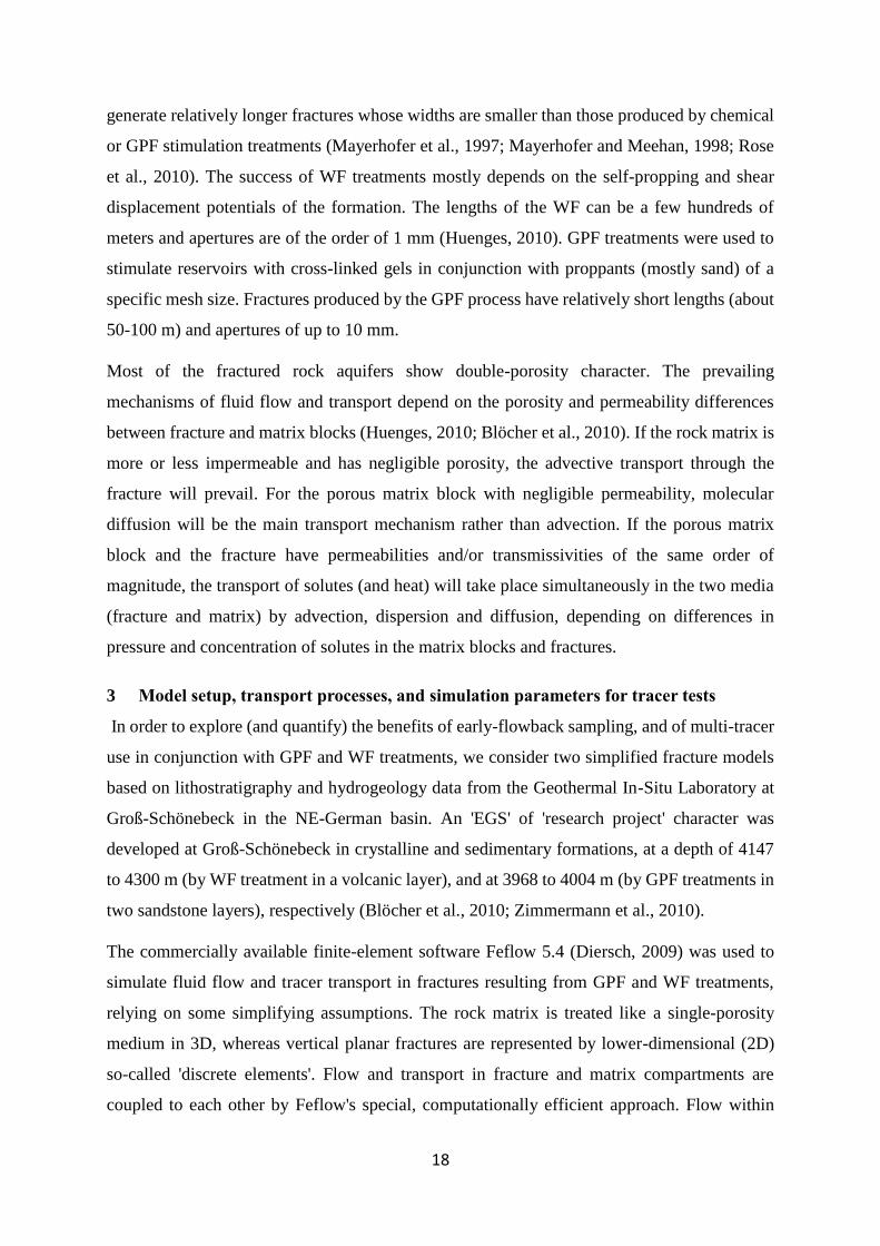
18

generate relatively longer fractures whose widths are smaller than those produced by chemical

or GPF stimulation treatments (Mayerhofer et al., 1997; Mayerhofer and Meehan, 1998; Rose

et al., 2010). The success of WF treatments mostly depends on the self-propping and shear

displacement potentials of the formation. The lengths of the WF can be a few hundreds of

meters and apertures are of the order of 1 mm (Huenges, 2010). GPF treatments were used to

stimulate reservoirs with cross-linked gels in conjunction with proppants (mostly sand) of a

specific mesh size. Fractures produced by the GPF process have relatively short lengths (about

50-100 m) and apertures of up to 10 mm.

Most of the fractured rock aquifers show double-porosity character. The prevailing

mechanisms of fluid flow and transport depend on the porosity and permeability differences

between fracture and matrix blocks (Huenges, 2010; Blöcher et al., 2010). If the rock matrix is

more or less impermeable and has negligible porosity, the advective transport through the

fracture will prevail. For the porous matrix block with negligible permeability, molecular

diffusion will be the main transport mechanism rather than advection. If the porous matrix

block and the fracture have permeabilities and/or transmissivities of the same order of

magnitude, the transport of solutes (and heat) will take place simultaneously in the two media

(fracture and matrix) by advection, dispersion and diffusion, depending on differences in

pressure and concentration of solutes in the matrix blocks and fractures.

3 Model setup, transport processes, and simulation parameters for tracer tests

In order to explore (and quantify) the benefits of early-flowback sampling, and of multi-tracer

use in conjunction with GPF and WF treatments, we consider two simplified fracture models

based on lithostratigraphy and hydrogeology data from the Geothermal In-Situ Laboratory at

Groß-Schönebeck in the NE-German basin. An 'EGS' of 'research project' character was

developed at Groß-Schönebeck in crystalline and sedimentary formations, at a depth of 4147

to 4300 m (by WF treatment in a volcanic layer), and at 3968 to 4004 m (by GPF treatments in

two sandstone layers), respectively (Blöcher et al., 2010; Zimmermann et al., 2010).

The commercially available finite-element software Feflow 5.4 (Diersch, 2009) was used to

simulate fluid flow and tracer transport in fractures resulting from GPF and WF treatments,

relying on some simplifying assumptions. The rock matrix is treated like a single-porosity

medium in 3D, whereas vertical planar fractures are represented by lower-dimensional (2D)

so-called 'discrete elements'. Flow and transport in fracture and matrix compartments are

coupled to each other by Feflow's special, computationally efficient approach. Flow within

19

WF-type fractures is assumed to obey the 'cubic law' (Tsang, 1992); flow within the matrix, as

well as within GPF-type fractures, is assumed as Darcian. Thus, GPF-type fractures are treated

almost like an ordinary porous medium, which (with the exception of solute exchange with the

adjacent rock matrix) is similar to the 'push-pull' test situation considered by Schroth et al.

(2001), with some limitations to be discussed in the next section. Solute transport in fractures,

and within rock matrix is assumed as advective-dispersive, with a number of additional

processes at fluid-solid interfaces as described below (adsorption-desorption onto/from matrix

rock, or proppant coatings; matrix diffusion). The model has to be 3D because of its fracture

(approximately radial) and matrix (approximately linear) flow and transport components. The

assumption of horizontal and vertical symmetry and neglecting gravity effects means that we

need to consider only one-quarter of the fracture plane, one-half of the fracture aperture or

thickness and 1/8 of its adjacent matrix block (similar to the model used by Ghergut et al.,

2013b for parallel-fracture systems). The geometry of model compartments (fracture and

matrix block) and the hydrogeological parameter distribution for the WF and GPF target layers

are shown in Fig. 2.1.1. The assumption of isotropic permeability (described by a single scalar

value for each compartment) is rather unrealistic, but it does not influence the parameter

sensitivity behavior of simulated tracer signals. Further, we assume isothermal conditions; the

hydraulic conductivity values listed in Fig. 2.1.1 corresponds to a temperature of 120°C,

assumed to prevail during tracer injection and early flowback, as a transient 'equilibrium'

between native reservoir conditions (~160°C) and injectate temperature (~15°C).

20

Figure 2.3.1: 3D model domain and hydrogeological parameter distribution (after Blöcher et al., 2010)

Table 1: Values of matrix and fracture parameters in WF and GPF model

Water fracture (WF) Gel proppant fracture

(GPF)

Hydraulic

conductivity

Stimulated layer 3.2×10-9 m/s 6.4×10-8 m/s

Fracture arrest

layer

3.2×10-9 m/s 1.6×10-9 m/s

Porosity Stimulated layer 0.1% 3%

Fracture arrest

layer

0.5% 1%

½ Fracture height 100m 60m

½ Fracture length 190m 60m

Fracture porosity 100% 30% to 60%

Fracture aperture (WF)/thickness

(GPF)

0.18mm to 1.08mm 2mm to 24mm

Fracture apertures were varied between 0.2 mm and 24 mm, the lower of these values being

regarded as more representative for fractures resulting from WF treatments, and the higher

values for fractures resulting from GPF treatments (Table 1). Within GPF-type fractures,

21

proppant-packing porosity was varied between 30% and 60%. Longitudinal dispersivities

within fractures were varied in the range of few meters, their effect on simulated tracer signals

was considered (see next section). Transverse dispersivities were assumed to be twenty times

lower. Dispersivity values for the rock matrix, likely in the range of centimeters-decimeters,

did not show any notable influence on simulated tracer signals, as advective penetration of the

matrix remained negligible. In the sequel, whenever the term 'dispersivity' is used, it pertains

to longitudinal dispersivity within fractures. In order to avoid confusion between 'total

aperture' and 'effective aperture' (equal to the product of 'total aperture' and intra-fracture

porosity), we prefer to reserve the term 'aperture' for the WF type (with 100% porosity), and

denote the total aperture of a GPF-type fracture as 'thickness'. The notion of aperture is

context-dependent; the systematic difference, both in theory and in field measurements,

between 'hydraulic aperture', 'tracer aperture', and 'tracer-hydraulic aperture' was explained by

Tsang (1992) as the difference between 'cubic law aperture', 'mass balance aperture', and

'frictional loss aperture'; aperture measurements should always be regarded as context

dependent (Berkowitz, 2002). In the sense of Tsang (1992), the findings in the present paper

pertain to 'mass balance aperture' only.

For tracer tests conducted in conjunction with WF and GPF treatments, we consider three

classes of tracers: conservative (in particular, non-sorbing) tracers, matrix-sorptive tracers

(MST), and proppant-sorptive tracers (PST). In any kind of test, whether with WF or GPF

treatments, at least one conservative tracer shall always be injected; within the conservative-

tracer class, diffusion coefficients were varied in order to probe the usefulness of matrix

diffusion processes for parameter determination from early flowback signals (the result being

largely negative). For obvious reasons, PST can be used only with GPF treatments, whereas

MST can in principle be used both with WF and with GPF treatments. The idea that PST and

MST can -and ought to be assumed different from each other (distinct groups of chemicals) is

justified by the chemical specificity of adsorption processes: roughly speaking, “different

species have a different adsorption affinity to different solid surfaces”. Not only should MST

differ from PST, MST for volcanics will likely be different from MST for sandstone or

claystone. Proppant particles can be prepared with specific coatings to ensure sorptivity for

certain tracers.

Given the relatively low flow velocities, the processes of tracer adsorption-desorption

(onto/from rock matrix or proppants) can be assumed to be at equilibrium, and given the

typically low tracer concentrations, sorption distribution laws can be assumed as linear (Freeze

22

and Cherry, 1979), which allows the effects of sorption-desorption on tracer transport to be

described simply by a dimensionless retardation factor (Bouwer, 1991; Kinzelbach and Rausch,

1995; Schroth et al., 2001), defined as:

𝑅 = 1 + 𝜌 × 𝐾𝑑 ×1−𝑛

𝑛= 1 + κ ×

1−n

n… … … . . (1)

where:

n = porosity of the flow medium (either rock matrix, for MST, or proppant packing, for PST)

𝜌 = intrinsic density of solid-phase material (either rock, or proppants)

𝐾𝑑 = sorption distribution coefficient (slope of linear segment of adsorption isotherm, Freeze

and Cherry, 1979)

𝜅 = 𝜌 × 𝐾𝑑 = dimensionless sorption distribution coefficient

The retardation factor R is not an intrinsic tracer property, but it also depends on the porosity

of the transport medium; thus, strictly speaking, R-values cannot be varied independently of

porosity. Laboratory tests on tracer sorptivity, conducted prior to tracer use in field tests,

measure 𝐾𝑑 or 𝜅, not R values. However, some of the simulation results presented in the next

sections are better described in terms of R.

4 Spatial discretization and hydraulic treatment of injection-flowback tests

The horizontal extent of the model domain was chosen to be at least twice the maximum tracer

travel distance. The fracture and matrix block are shown in Fig. 2.1.1 was discretized by up to

58280 elements. A stronger retardation by adsorption/desorption implies a shorter travel

distance for that particular tracer species. This implies that spatial discretization (and hence

numerical dispersion) may vary from tracer to tracer. The numerical dispersion was

investigated in a separate study (Karmakar, in prep., Chapter 2, part 3).

The timing of tracer pulse and fluid (chaser) injection and flowback for both WF and GPF

treatments are presented in Fig. 2.1.2. The total simulation time of up to 2 days were discretized

by up to 2100 time steps of variable duration, resulting from time-step control by predictor-

corrector schemes implemented in FEFLOW. The initial time step was set to 10-9 day, and the

time step increase factor was limited to 1.2, as injection duration was very small, and the shift

from injection to pumping was assumed to take place over a very short time interval.

23

Figure 2.4.1: Fluid and tracer injection-flowback in GPF and WF treatments. The transition from

constant injection to constant flowback was approximated as linear (dashed-line segment); its duration

is enlarged for better recognition. In the simulations, the transition spans only 1/60 of Tpush.

Injection rate and duration were set as similar for all tracer species corresponding to a chaser

injection volume of about half the typical fracture. This is a reasonable compromise between

the requirement that 'most tracers stay within the fracture' and the fact that fracture aperture is

not known prior to the test. The chaser fluid (water) was injected in pulses to move the tracer

to a certain distance inside the fracture. An advantage of this particular SW approach is that it

does not rely on substantial advective penetration into the rock matrix. The flowback volume

(Fig. 2.1.2) can be significantly larger than the tracer chaser volume injected immediately prior

to it. The flowback results from pressure buildup by the entire treatment process, with total

injectate volumes being much larger than the tracer-chaser volume (especially for WF

treatments). We recall that tracer and chaser are added only at the end of the treatment. In fact,

flowback rate and duration are independent of the tracer-chaser injection rate and duration.

Without external control, flowback would start at high rates and then decline more or less

exponentially, but in practice often some control is applied to maintain it at an approximately

constant rate; thus, for simplicity, the scheme is shown in Fig. 2.1.2 was used.

24

5 Parameter interplay, and numerical simulations

The study by Schroth et al. (2001) on the in-situ evaluation of solute retardation using SW

push-pull indicates that in a homogeneous single-porosity medium tracer 'pull' signals depend

on porosity, thickness, and longitudinal dispersivity through the following product

(porosity × thickness) × (dispersivity squared), or (2)

(effective aperture) × (dispersivity squared),

It, therefore, follows that these three parameters cannot be determined independently from each

other. Dispersivity has a stronger influence than porosity or thickness – a fact that can become

useful as will be seen in the next section. In groundwater remediation application considered

by Schroth et al. (2001), this hydrogeological parameter interplay was not an issue, since the

aquifer thickness and porosity were known in advance of conducting the SW tracer push-pull

tests, and the unknown parameters were aquifer dispersivity and solute retardation. By contrast,

in the present study, all these parameters are unknown (three parameters for GPF: thickness,

porosity, dispersivity; two parameters for WF: aperture, dispersivity); however, the tracer-

proppant/rock sorptivity behavior is assumed as known in advance.

The closed-form approximation to tracer 'pull' signals used by Schroth et al. (2001) may not be

applicable to our WF and GPF tracer test scenarios. In fact, formulae (9) - (11) used by Schroth

et al. (2001, pp. 107-108) are valid only in the low-dispersivity limit, a requirement very likely

violated by fractures resulting from GPF or WF treatments in natural geothermal reservoirs.

Consequences of parameter interplay on the parameter estimation from measured tracer signals

in natural systems need not be as dramatic as suggested by product (2). As an example, the

product formula implies that a tenfold increase in dispersivity will produce the same effect on

tracer signals as a 100-fold increase in porosity, thickness, or effective aperture. However, with

porosity expected to be between 30% and 60%, and thickness or aperture ranging from ~1mm

to ~1cm, a 100x variation cannot actually occur. Thus the fact that dispersivity has a stronger

effect on SW tracer signals than the other parameters, in conjunction with relatively narrow

ranges for parameters like proppant-packing porosity, GPF thickness or WF aperture, may

allow to at least roughly estimate dispersivity without knowing the exact values of other

parameters. A possible workaround to parameter interplay is the use of semi-empirical

correlations between hydrogeological parameters to constrain the value of either dispersivity

as a function of fracture aperture and porosity (Horne and Rodriguez, 1981; Fossum and Horne,

1982; Pruess and Bodvarsson, 1984), or porosity as a function of permeability (Guimerà and

25

Carrera, 1997), or proppant-packing dispersivity as a function of proppant treatment protocols

(Tomac and Gutierrez, 2015).

Alternatively, it may be possible to make priori assumptions on the magnitude of the Peclet

number (Pe) of the overall transport scenario (with Pe defined as the ratio between tracer-

invaded fracture radius and longitudinal dispersivity). For the vast majority of transport

scenarios in fractured-porous media of practical relevance, Peclet numbers range between 8

and 20. Dispersion within fractures can result from multiple processes – the most significant

of which include: 'Taylor-Aris dispersion', 'roughness dispersion', 'aperture-variation

dispersion' (Bauget and Fourar, 2007); it is not possible to individually quantify these processes

from early-flowback observations. There is an important difference between the SW tracer test

scenario of Schroth et al. (2001) and the GPF and WF tracer test scenarios considered in the

present paper. Whereas the transport of conservative and PST in GPF-type fractures is

approximately similar to tracer transport in the 'aquifer cylinder' of Schroth et al. (2001), the

transport of

(i) 'matrix-diffusive' tracers in thin WF-type fractures and

(ii) MST in any fracture type

does not fit into the model considered by Schroth et al (2001); the latter model excludes tracer

exchange across 'cylinder' top and bottom (corresponding to fracture walls, or the fracture-

matrix interface). Owing to tracer flux across fracture walls, WF aperture and GPF thickness

are expected to influence MST and possibly 'matrix-diffusive' signals in addition to the product

parameter (2). As to matrix diffusion, one should not expect it to have a notable effect in short-

term tests in GPF-type fractures, but it might have some impact in thin WF-type fractures.

Various studies (Kocabas and Horne, 1987; Pruess and Doughty, 2010; Jung and Pruess, 2011;

Maier and Kocabas, 2013) indicate that thin-fracture apertures can be estimated from SW push-

pull tests using conservative tracers or heat exchange, relying on matrix diffusion; however,

considerably longer observation times are required than those considered in this early-flowback

study. The process of MST exchange at fracture walls largely resembles that of matrix

diffusion, but unlike matrix diffusion, equilibrium is attained within a very short time. It is,

therefore, reasonable to expect that MST may be helpful for estimating WF aperture and GPF

thickness independently of other hydrogeological parameters.

26

Based on above considerations, the numerical simulations of tracer tests in fractures resulting

from GPF and WF treatments were designed to:

1.) probe the effects of dispersivity, and its interplay with porosity and thickness or aperture,

on conservative tracer signals in GPF and WF (for obtaining a rough estimate of dispersivity);

2.) explore the effects of porosity and thickness or aperture in MST in GPF and WF (for

determining GPF thickness and WF aperture);

3.) explore the effects of porosity and thickness on PST in GPF (for determining proppant-

packing porosity in GPF).

6 Results

In this section, we present numerical simulation results focusing on the following four issues:

(i) how does each parameter (dispersivity, WF aperture, GPF thickness and porosity) influence

the 'peak arrival time', and the early amplitude of simulated tracer signals? Signal tails are

ignored, since parameter determination is based only on early flowback;

(ii) is the influence monotonic with respect to a parameter over its relevant range of values?

(iii) if parameter interplay occurs, to what extent does it impede parameter determination?

(iv) do the signals of sorptive tracers show less interplay and/or improved sensitivity to relevant

parameters, compared to conservative-tracer signals?

The slight 'bump' at the beginning of flowback signals, seen in some of the simulated tracer

signals, is due to the representation of injection-flowback hydraulics. The rates of injection and

flowback were set as constant, with a short linear transition interval between them (indicated

by dashed-line segments on Fig. 2.1-2); instead of letting the variable flowback rate naturally

adjust to the actual outflow boundary condition. This 'bump' does not affect parameter

sensitivity or estimation since it is not associated with any special ‘arrival time’ that may be

used for parameter determination.

6.1 Conservative-tracer signals during early flowback

Figs. 2.1- 3 and 2.1- 4 demonstrate the influence of dispersivity (αL) on conservative-tracer

signals during early flowback in GPF-type fractures and its interplay with fracture thickness

and proppant-packing porosity. In Fig. 2.1.3, porosity is kept fixed while thickness is varied

whereas in fig. 4 the thickness is kept fixed while porosity is varied. As expected from the

discussion in a previous section, the product-type parameter interplay (2) is seen to occur, but

27

the influence of dispersivity is significantly stronger than that of thickness or porosity. Thus,

dispersivity can be roughly estimated, though additional / a priori knowledge from other

sources would be helpful. Signal amplitude decreases monotonically with increasing

dispersion, whereas dispersion influence on 'peak arrival time' is insufficient for parameter

estimation purposes.

Figure 2.6.1: Simulated signals of conservative tracers during GPF flowback: the effect of dispersion

processes (expressed by eight different values of longitudinal dispersivity αL, as indicated by signal

labels, in meters), shown for two different values of GPF thickness (solid line: 12mm, dashed-dotted

line: 20mm), with a fixed value of GPF porosity (45%).

0.1

0.12

0.14

0.16

0.18

0.2

0.3 0.4 0.5 0.6 0.7 0.8 0.9 1

Co

nce

ntr

atio

n m

g/L

Time (days) after tracer injection (with flowback starting at 0.3 days)

28

Figure 2.6.2: Simulated signals of conservative tracers during GPF flowback: the effect of dispersion

processes (expressed by eight different values of longitudinal dispersivity αL, as indicated by signal

labels, in meters), shown for three different values of GPF porosity (solid line: 30%, dashed line: 45%,

dashed-dotted line: 60%), with a fixed value of GPF thickness (12mm).

Fig. 2.1.4 demonstrates the influence of dispersion and fracture aperture on conservative-tracer

signals during early flowback in WF-type fractures. Unlike in the GPF case, there is a

significant monotonic increase of 'peak arrival time' with decreasing dispersivity, whereas

aperture is seen to have no significant influence on 'peak arrival time'. There is the interplay

between dispersivity and aperture with regard to signal amplitude, but the dispersivity value

identified based on 'peak arrival time' can be used to determine aperture. Unlike in the GPF

case, signal slopes vary strongly, both in time and in parameter space.

0.09

0.11

0.13

0.15

0.17

0.19

0.21

0.3 0.4 0.5 0.6 0.7 0.8 0.9 1

Co

nce

ntr

atio

n m

g/L

Time (days) after tracer injection (with flowback starting at 0.3 days)

29

Figure 2.6.3: Simulated signals of conservative tracers during WF flowback: the distinct effects of

fracture aperture (with values represented by different shadings as shown by legend) and of

longitudinal dispersivity (solid line: 7m, dash-dotted line: 5m).

6.2 MST signals during early flowback

In Figs. 2.1.8–10, the transport of MST in GPF-type fractures is explored from two different

angles: (1) comparison between MST and matrix diffusion processes; and (2) parameter

determination. Fig. 6 (produced with fixed values of GPF thickness and porosity) demonstrates

that increasing MST sorptivity lowers the tracer signal peak amplitude (approximately

inversely proportional to 𝑅1

2⁄ during early flowback), without influencing the apparent 'peak

arrival time'. This is somewhat analogous to the effects of increasing diffusion coefficients in

the context of matrix diffusion in SW push-pull tests (cf. Ghergut et al. 2013b). Fig. 2.1.9

illustrates that the sensitivity to fracture thickness improves with increasing sorptivity; this was

confirmed over the entire parameter range of interest. The thickness sensitivity of any MST is

greater than that of a non-sorptive tracer, and increases with decreasing thickness; on the other

hand, signal amplitude increases monotonically with increasing thickness, and decreases with

0.06

0.08

0.10

0.12

0.14

0.16

0.18

0.20

0.22

0.24

0.3 0.4 0.5 0.6 0.7 0.8 0.9 1

Co

nce

ntr

atio

n m

g/L

Time (days) after tracer injection (with flowback starting at 0.3 days)

af1.08mm af1.08mm

af0.90mm af0.90mm

af0.72mm af0.72mm

af0.54mm af0.54mm

af0.36mm af0.36mm

af0.18mm af0.18mm

30

increasing sorptivity. Fig. 2.1.8 demonstrates that the MST signals are independent of

proppant-packing porosity; and the GPF thickness can be determined independently of

porosity.

Figure 2.6.4: Simulated signals of various MST (characterized by different Kd values) during GPF

flowback, at a fixed value of GPF thickness (12mm) and proppant-packing porosity 30%). Signals are

labeled by the retardation factor R, instead of Kd values the signal of a conservative (non-sorptive,

Kd=0, R=1) tracer is shown for comparison.

0.03

0.05

0.07

0.09

0.11

0.13

0.15

0.17

0.19

0.3 0.4 0.5 0.6 0.7 0.8 0.9 1

Co

nce

ntr

atio

n m

g/L

Time (days) after tracer injection (with flowback starting at 0.3 days)

R=1 R=2 R=5 R=10

R=16

R=25

R=40 R=60

31

Figure 2.6.5: Simulated signals of two MST during GPF flowback: the effect of GPF thickness (values

are indicated as signal labels, in mm), with a fixed value of proppant-packing porosity (45%), shown

for two tracer species, a less sorptive one (dimensionless 𝜅= 0.9), and a more sorptive one

(dimensionless 𝜅=1.52).

0.060

0.065

0.070

0.075

0.080

0.085

0.090

0.095

0.3 0.34 0.38 0.42 0.46 0.5

Co

nce

ntr

atio

n m

g/L

Time (days) after tracer injection (with flowback starting at 0.3 days)

k=1.52

k=0.90

tF=4

tF=24 tF=16

tF=12

tF=20

tF=8

32

Figure 2.6.6: Simulated signals for one MST (characterized by dimensionless κ= 1.5) during GPF

flowback: the effect of GPF thickness (values are indicated as signal labels, in mm), with two values of

GPF porosity (solid line: 30%, broken line: 60%)

For MST signals in WF-type fractures (not shown here), a largely similar behavior was found.

Sensitivity to aperture is improved, compared to that for non-sorptive tracers, and sensitivity

increases with decreasing aperture. On the other hand, signal amplitude increases

monotonically with increasing thickness and decreases with increasing sorptivity. Deviations

from the above-described behavior (and a slight influence on apparent 'arrival times') are seen

to occur for values outside the plausible range for GPF thickness or WF aperture.

6.3 PST signals during early flowback in GPF fractures

Finally, the transport of PST in GPF-type fractures is explored from two different angles i.e.,

parameter interplay, and porosity determination. Fig. 2.1.11 illustrates the interplay between

GPF-type fracture thickness and proppant-packing porosity. Signal amplitude decreases with

increasing fracture thickness but increases with increasing porosity.

0.06

0.065

0.07

0.075

0.08

0.085

0.3 0.34 0.38 0.42 0.46 0.5

Co

nce

ntr

atio

n m

g/L

Time (days) after tracer injection (with flowback starting at 0.3 days)

tF=4

tF=24

tF=16 tF=12

tF=20

tF=8

33

Fig. 2.1.10 demonstrates that once the value of GPF-type fracture thickness was identified

(using an MST tracer as described in section 6.2), the proppant-packing porosity can be

determined, provided fracture thickness is about ~1 cm or higher. If GPF-type fracture

thickness is less than 0.5cm (which is implausible), PST signal sensitivity to porosity becomes

too low.

Figure 2.6.7: Simulated signals for one PST (characterized by dimensionless κ=40) during GPF flowback:

the effects of GPF thickness and of GPF porosity (solid lines: 35%, broken lines: 55%) illustrate

parameter interplay.

0.07

0.09

0.11

0.13

0.15

0.17

0.19

0.21

0.3 0.4 0.5 0.6 0.7 0.8 0.9 1

Co

nce

ntr

atio

n m

g/L

Time (days) after tracer injection (with flowback starting at 0.3days)

tF4mm tF4mm

tF8mm tF8mm

tF12mm tF12mm

tF16mm tF16mm

tF20mm tF20mm

tF24mm tF24mm

34

Figure 2.6.8: Simulated signals for one PST (characterized by dimensionless κ =40) during GPF flowback:

the effect of GPF thickness (values are indicated in mm), and the effect of GPF porosity (gray tones,

from light: 30%, to dark: 60%), illustrating the increase of porosity sensitivity with increasing thickness.

7 Discussion, and recommendations for future tracer tests

Owing to flow-field reversal by the SW test configuration, two 'unusual' behaviors occur,

opposite to those from inter-well tracer tests: 'retardation' factors are not directly reflected by

the apparent 'arrival times' (cf. discussion in Ghergut et al., 2013a), whereas dispersion

determines the apparent 'arrival time'. Moreover, this latter effect is strong enough for

conservative tracers in thin WF-type fractures to enable dispersivity and aperture determination

independently of each other. For thicker, GPF-type fractures, a stronger parameter interplay is

found between dispersivity, fracture thickness and proppant-packing porosity. However, a

rough estimation of dispersivity from conservative tracer signals is still possible since

dispersivity effects are stronger than those of GPF thickness and proppant-packing porosity.

Once dispersivity is identified (by this or some different approach as suggested in section 5),

0.08

0.1

0.12

0.14

0.16

0.18

0.2

0.22

0.3 0.4 0.5 0.6 0.7 0.8 0.9 1

Co

nce

ntr

atio

n m

g/L

Time (days) after tracer injection (with flowback starting at 0.3 days)

2mm4mm

8mm

16mm

35

GPF-type fracture thickness and proppant-packing porosity can be determined independently

of each other, if suitable MST and PST data are available. The use of an MST enables thickness

determination; and a PST enables proppant-packing porosity determination if the thickness is

not too small. For WF-type fractures, aperture determination is possible with conservative

tracers alone, but the use of MST improves sensitivity. Parameter determination for GPF-type

fractures only becomes possible with MST and PST.

Regarding the use of conservative tracer pairs with contrasting diffusivity, simulations have

shown that matrix diffusion effects are far too weak to enable parameter inversion from early

flowback signals. Alternatively, heat could be used as a 'matrix-diffusive tracer' instead of

solute tracers, owing to heat diffusivities being much higher than solute diffusivities (Kocabas

and Horne, 1987; Pruess and Doughty 2010; Jung and Pruess, 2011; Maier and Kocabas, 2013).

However, during early flowback following multiple injectate slugs with different temperatures,

it may be difficult to use “heat” for determining fracture parameters.

Based on Figs. 2.1.3–5, 2.1.8 and 2.1.10 one can make some recommendations regarding the

timing and frequency of tracer signal sampling. For WF-type fractures, dense sampling at the

beginning of flowback (at least 30 samplings during the very first day, i.e. before recovering

the first 1/10 of the injected chaser volume) is necessary, if both dispersivity and aperture are

to be determined. By contrast, for GPF-type fractures, sparse uniform sampling (~10 samplings

uniformly distributed over a flowback volume of the same order as the chaser volume) should

suffice for fracture parameter estimation – if suitable MST and PST are available. For WF-type

fractures essential tracer information can be contained in the very first hours of flowback and

for GPF-type fractures, the flowback corresponding to a recovery between 1/3 and 2/3 of

chaser volume is likely to yield the most useful information.

To identify the minimum sorptivity (minimum κ value) required to induce sufficient contrast

between measurable tracer signals for different values of target parameters, the scheme to

follow is: a p% change in a target-parameter value produces c% change in the signal of a

conservative tracer, and a s% change in the signal of a sorptive tracer, s being a function of κ.

One then needs to find out the minimum value of κ that renders s significantly higher than c.

This value cannot be prescribed in a universal manner because the very meaning of

'significantly higher' depends on how tracer signals can be sampled and measured, a process

always affected by various errors. In any case, the higher the value of κ, the higher is the

sensitivity improvement. On the other hand, the higher the tracer's retardation, the lower is its

36

fracture invasion, and consequently a poorer capability for characterizing the fracture as a

whole. In principle, this could be compensated by increasing the chaser volume (i.e., by

injecting sorptive tracers earlier than conservative tracers). The effect of different injection

durations (different chaser volumes) on tracer signals was investigated in a parallel study

(Karmakar et al., 2015).

Fracture thicknesses based on neutron ray detection and the use of proppants with activated

coatings (McDaniel et al., 2009) can provide enough data to determine fracture opening during

the EGS development and monitoring phases. However, the neutron rays commonly detected

by gamma probes may be affected by the presence of neutron-ray absorbing or emitting

substance in the rock mass or by barriers across the fracture opening that impair detection. In

the latter case, a tracer-based SW test would be advantageous for obtaining reliable data. The

early tracer signal can be employed to characterize fracture thickness and porosity by using

two tracers that are only retarded by either the proppant or the matrix. Variable injection rates

were found to be effective during WF stimulation rather than a constant flow rate (“cyclic

stimulation”, Zimmermann et al, 2010). The tracer-based procedure described in the present

paper is also applicable in such cases; tracers should be added shortly before the end of the last

injection cycle.

In summary, this simulation study has produced two significant results: (1) water fracture

aperture can be effectively evaluated based on early-time tracer signals of a conservative tracer;

and (2) by using the combination of matrix sorptive and proppant sorptive tracers, it is possible

to estimate fracture thickness and porosity in gel proppant fractures from a single test.

The injection and flowback of a small fluid volume, and thus little dilution of the injected

tracers, has three practical advantages: (1) there is no need to inject large tracer quantities; (2)

one does not have to wait for the tails of the test signals; and (3) the field and laboratory

monitoring of the tracer signals does not have to be conducted for ultra-low tracer

concentrations, which is known to be a major challenge, with the highly-mineralized and

especially high organic content fluids typically encountered in the NE German Basin at 3-5 km

depth.

Acknowledgments: The first author gratefully acknowledges continued financial support from

the DAAD (German Academic Exchange Service) to pursue his Ph.D. work. This work also

benefited from long-term financial and technical support granted by the Federal German

37

Ministry for Economic Affairs and Energy (BMWi) within the project TRENDS (2014-2018,

FKZ 0325515), as well as by Baker Hughes (Celle) and the Lower Saxonian Science and

Culture Ministry (MWK Niedersachsen) within the interdisciplinary research project “gebo -

Geothermal Energy and High-Performance Drilling” (2009-2014). Last, not least, the authors

gratefully acknowledge the reviewers Dr. Marcelo Lippmann, Mr. Michael G. Shook, as well

as the Editors for their valuable help in improving this manuscript.

References

Bauget, F., Fourar, M., 2007. Convective Dispersion in a Real Fracture. In: Proceedings 32nd

Workshop on Geothermal Reservoir Engineering, Jan. 22-24, 2007, Stanford Univ. (CA),

SGP-TR-183.

Berkowitz, B., 2002. Characterizing flow and transport in fractured geological media: A review.

Adv. in Water Resour. 25, 861-884.

Blöcher, G., Zimmermann, G., Moeck, I., Brandt, W., Hassanzadegan, A., Magri, F., 2010. 3D

numerical modeling of hydrothermal processes during the lifetime of a deep geothermal

reservoir. Geofluids 10, 406-421.

Bouwer, H., 1991. Simple Derivation of the Retardation Equation and Application to Preferential

Flow and Macrodispersion. Ground Water 29(1), 41-46.

Dean, C., Reimus, P., Oates, J., Rose, P., Newell, D., Petty, S., 2015. Laboratory experiments to

characterize cation-exchanging tracer behavior for fracture surface area estimation at

Newberry Crater, OR. Geothermics 53, 213–224.

Diersch, H.-J., G., 2009. FEFLOW 5.4: finite element subsurface flow and transport simulation

system. Reference manual. DHI-WASY Ltd., Berlin, Germany, 292 pp

Fossum, M. P., Horne, R. N., 1982. Interpretation of Tracer Return Profiles at Wairakei Geothermal

Field Using Fracture Analysis. Geothermal Research Council Transactions 6, 261-264.

Freeze, R.A., Cherry, J.A., 1979. Groundwater. Prentice-Hall, Englewood Cliffs, NJ, 604 pp.

Ghergut, I., Behrens, H., Sauter, M., 2013a. Can Peclet numbers depend on tracer species? going

beyond SW test insensitivity to advection or equilibrium exchange. In: Proceedings 38th

Workshop on Geothermal Reservoir Engineering, Stanford Univ. (CA), SGP-TR-198, 326-

335.

Ghergut, I., Behrens, H., Sauter, M., 2013b. Single-well tracer push-pull test sensitivity to fracture

aperture and spacing. In: Proceedings 38th Workshop on Geothermal Reservoir Engineering,

Stanford Univ. (CA), SGP-TR-198, 295-308.

Ghergut, I., Behrens, H., Sauter, M., 2014. Tracer-based Quantification of Individual Frac

Discharge in Single-well Multiple-frac Backflow: Sensitivity Study. Energy Procedia 59, 235–

242.

38

Guimerà, J., Carrera, J. 1997. On the interdependence of transport and hydraulic parameters in low

permeability fractured media. In: Hard Rock Hydrosystems (Proceedings of Rabat Symposium

S2, May 1997). IAHS Publ. no. 241, pp. 123-133.

Haggerty, R., McKenna, S.A., Meigs, L.C., 2000. On the late-time behavior of tracer test

breakthrough curves. Water Resources Research 36(12), 3467–3479.

Horne, R. N., Rodriguez, F. J., 1981. Dispersion in Tracer Flow in Fractured Geothermal Systems.

In: Proceedings 7th Workshop on Geothermal Reservoir Engineering, Stanford University

(CA), SGP-TR-55, 103-107.

Horne, R.N., 1985. Reservoir Engineering Aspects of Reinjection. Geothermics 14, 449-457.

Huenges, E. (Ed.), 2010. Geothermal Energy Systems: Exploration, Development and Utilization,

Weinheim:Wiley-VCH. 463pp.

Jung, Y., Pruess, K., 2011. A closed-form analytical solution for thermal single-well injection-

withdrawal tests. Water Resources Research 48(3), DOI: 10.1029/2011WR010979.

Karmakar, S. in preparation, Single-well tracer push-pull method development for characterizing

subsurface processes. Ph.D. Thesis, University of Göttingen, Germany.

Karmakar, S., Ghergut, I., Sauter, M., 2015. EGS in sedimentary basins: sensitivity of early-

flowback tracer signals to induced-fracture parameters. Energy Procedia 76, 223-229.

doi:10.1016/j.egypro.2015.07.906

Kinzelbach, W., Rausch, R., 1995. Grundwassermodellierung: Eine Einführung mit Übungen.

Gebr. Borntraeger, Berlin Stuttgart, pp. 39-40.

Kocabas, I., Horne, R.N., 1987. Analysis of Injection-Backflow Tracer Tests in Fractured

Geothermal Reservoirs. In: Proceedings 12th Workshop on Geothermal Reservoir Engineering,

Stanford University (CA), SGP-TR-109.

Maier, F., Kocabas, I., 2013. Efficient analytical solution for parameter estimation of push shut-in

pull experiments in an idealized single fracture system. In: Proceedings 38th Workshop on

Geothermal Reservoir Engineering, Stanford University (CA), SGP-TR-198.

Mayerhofer, M.J., Meehan, D.N., 1998. Waterfracs: results from 50 Cotton Valley wells. Society

of Petroleum Engineers Annual Technical Conference, Paper 49104, New Orleans, Louisiana,

27-30 September 1998.

Mayerhofer, M.J., Richardson, M.F., Walker, R.N.Jr., Meehan, D.N., Oehler, M.W., Browning,

R.R.Jr., 1997. Proppants? We don't need no proppants. Society of Petroleum Engineers

Annual Technical Conference, Paper 38611, San Antonio, Texas, 5-8 October 1997.

McDaniel, R.R., Holmes, D.V., Borges, J.F., Bajoie, B.J., Peeples, C.R., Gardner, R.P., 2009.

Determining Propped Fracture Width from a New Tracer Technology. SPE paper 119545. SPE

Hydraulic Fracturing Technology Conference, The Woodlands, Texas, USA, 19-21 January,

2009.

39

Nottebohm, M., Licha, T., Ghergut, I., Nödler, K., Sauter, M., 2010. Development of

Thermosensitive Tracers for Push-Pull Experiments in Geothermal Reservoir

Characterization. In: Proceedings World Geothermal Congress Bali, Indonesia), 6pp.

Pruess, K., Bodvarsson, G.S., 1984. Thermal Effects of Reinjection in Geothermal Reservoirs with

Major Vertical Fractures. J. of Petroleum Technology 36, 1567-1578.

Pruess, K., Doughty, C., 2010. Thermal single-well injection-withdrawal tracer tests for

determining fracture-matrix heat transfer area. In: Proceedings 35th Workshop on Geothermal

Reservoir Engineering, Stanford University (CA), SGP-TR-188.

Pruess, K., 2002. Numerical Simulation of Multiphase Tracer Transport in Fractured Geothermal

Reservoirs. Geothermics 31, 475-499.

Rose, P., Mella, M., Kasteler, C., Johnson, S.D., 2004. The Estimation of Reservoir Pore Volume

from Tracer Data. In: Proceedings 29th Workshop on Geothermal Reservoir Engineering, Jan.

26-28, 2004, Stanford Univ. (CA), SGP-TR-175.

Rose, P., Leecaster, K., Clausen, S., Sanjuan, R., Ames, M., Reimus, P., Williams, M., Vermeul,

V., Benoit, D., 2012. A Tracer Test at the Soda Lake, Nevada Geothermal Field Using a

Sorbing Tracer. In: Proceedings 37th Workshop on Geothermal Reservoir Engineering, Jan. 30

– Feb. 1, 2012, Stanford Univ. (CA), SGP-TR-194.

Rose, P.E., Xu, T., Fayer, S., Pruess, K., 2010. Chemical Stimulation for EGS: the Use of Chelating

Agents at High pH for the Simultaneous Dissolution of Calcium Carbonate, Silicas, and

Silicates. In: Proceedings World Geothermal Congress, Bali, Indonesia, 04/2010, 1-11

Schroth, M.H., Istok, J.D., Haggerty, R., 2001. In situ evaluation of solute retardation using single-

well push-pull tests. Advances in Water Resources, 24, 105-117.

Singhal, B.B.S., Gupta, R.P., 2010. Applied Hydrogeology of Fractured Rocks (2nd ed.). Springer

408 pp.

Tomac, I., Gutierrez, M., 2015. Micromechanics of proppant agglomeration during settling in

hydraulic fractures. J. Petrol. Explor. Prod. Technol. 151, DOI 10.1007/s13202-014-0151-9.

Tsang, Y.W., 1992. Usage of 'Equivalent Apertures' for Rock Fractures as Derived From Hydraulic

and Tracer Tests. Water Resour. Res. 28(5), 1451-1455.

Zimmermann, G., Moeck, I., Blöcher, G., 2010. Cyclic waterfrac stimulation to develop an

enhanced geothermal system (EGS): Conceptual design and experimental results.

Geothermics 39, 59-69.

40

CHAPTER 2-PART 2: EGS in sedimentary basins: sensitivity of early-flowback tracer

signals to induced fracture parameters

Shyamal Karmakar*, Julia Ghergut, and Martin Sauter

Citation:

Karmakar, S., Ghergut, I., Sauter, M., 2015. EGS in sedimentary basins: sensitivity of early

flowback tracer signals to induced-fracture parameters. Energy Procedia 76, 223-229.

doi:10.1016/j.egypro.2015.07.906

Geoscience Centre of the University of Göttingen, Department of Applied Geology,

Goldschmidtstrasse 3, 37077 Göttingen, Germany

*Corresponding author: shyamal.karmakar@geo.uni-goettingen.de

41

Abstract

Short-term flowback signals from injection-flowback tracer test face a certain degree of

ambiguity in fracture parameter inversion from the measured signal of a single tracer. This

ambiguity can be overcome by combining different sources of information (lithostratigraphy,

and hydraulic monitoring) and concomitantly using several tracers with different transport

behavior. To improve the early-time characterization of induced fractures, of either gel-

proppant or waterfrac, we recommend using tracers of contrasting sorptivity to rock surfaces,

and to proppant coatings where applicable. We illustrate the application of such tracer

combinations using hydro- and lithostratigraphy data from the Geothermal In-situ Laboratory

at Groß Schönebeck, Germany.

42

1 Introduction

Artificial-fracture design, and fracture characterization during or after stimulation treatment is

a central aspect of many enhanced geothermal system (EGS) of both in gel-proppant (GPF) or

in water fracture (WF) type stimulation projects. Tracer testing is a standard method of

determining mass transport within a geothermal reservoir and can be a valuable tool in the

design and management of production and injection operations (Horne 1985, Pruess, 2002).

Various single well (SW) tracer test approaches had revealed a great promise for parameter

estimation in fractured georeservoir using characteristic discharge rate, ion exchange (Dean et

al 2015) as well as a sorptive tracer. Late-time tracer signals from SW injection-flowback tests

have been used mainly for inflow profiling for EGS developed in multi-zone reservoirs in the

NE-German basin (Ghergut et al 2014). However, the potential of using early flowback tracer

signal from SW test for fracture characterization remained unexplored so far. Furthermore, no

'effort-against-benefit' analysis has been undertaken in a more focused manner, leaving issues

like the above as a matter of subjective pondering. We explored and outlined the actual benefit

from early-flowback sampling and from using more than one tracer per fracture. Additionally,

what improvements to parameter sensitivity can we expect? Moreover, this paper sought the

answer for early-sampling frequency as a trade-off between 'too much effort' and 'too sparse

information', especially for the case of gel-proppant fractures (GPF), where early flowback

sampling is likely to pose greater difficulties. In this instance, this paper aims to provide greater

insight into the early time tracer signal- based parametric study for fracture characterization in

an EGS of deep crystalline and/or sedimentary formations.

Nomenclature

SW Single-well

GPF Gel-proppant fracture

WF Water fracture

PST Proppant sorptive tracer

MST Matrix sorptive tracer

k Sorption coefficient, a multiple of Henry sorption coefficient (Kd) and density

43

2 Gel proppant fracture and water fracture simulation parameters

In our three-dimensional discrete fracture reservoir model in Feflow5.4 (Diersch 2009) we used

lithostratigraphic and hydrogeological data of Groß Schönebeck, NE German basin (Blöcher et

al. 2010) at depths of -3968m to -4004m (sedimentary formation, 3% porosity, hydraulic

conductivity 6.4×10-9 ms-1) for the gel proppant fracture, and from -4147m to -4300m for the

water fracture reservoir (volcanic formation, 0.5% porosity, hydraulic conductivity 3.2×10-9

ms-1). The horizontal extent of a model domain defined as twice the maximum tracer travel

distance and the depth was implemented toward the y-axis. Tracer was injected as a short pulse

both in the gel-proppant and water fracture simulation. The chaser fluid was injected after pulse

injection to drag the tracer up to ≤ half fracture height. We conducted simulations following

forward modeling principle using fracture thickness values 2mm to 24 mm and fracture porosity

30% to 60% for gel-proppant treatment fracture and fracture aperture 0.1mm to 1.44mm for

water fracture (Huenges 2010) for the solute transport with different sorptivities, k (k= Henry

sorption coefficient, Kd × density). Two different sorptive tracers were used for gel-proppant

fracture viz. matrix sorptive or proppant sorptive. Injection volume estimated as ~half of the

fracture volume for both water fracture and gel-proppant fracture while injection duration and

rate remained unchanged. Sorptive tracer/s, together with a conservative tracer, was/were co-

injected as a short pulse in water fracture or gel-proppant fracture. Fracture flow in gel-proppant

fracture was treated as Darcy flow and for water fracture, cubic law for flow in the fracture and

Darcian flow in the matrix.

3 Conservative and sorptive tracer test in gel proppant fracture

3.1 Conservative tracer

Early time flow-back tracer signal showed higher tracer peak, for lower dispersion. Matrix

parameter and fracture porosity or different packing of proppant do not affect tracer signals

significantly. From this analogy, it showed that conservative tracer would be effective to

estimate dispersion of solute in fracture (Figure 2.2.1 and 2.2.2).

44

Figure 2.2.1: Conservative tracer flowback signals from different dispersivity and fracture thickness:

broken line- 4mm, solid line- 16mm

Figure 2.2.2: Conservative tracer flowback signals from different dispersivity and fracture porosity.

0.10

0.12

0.14

0.16

0.18

0.20

0.3 0.4 0.5 0.6 0.7 0.8 0.9 1

Co

nce

ntr

atio

n m

g/L

Time (days) after mass injection (flowback start at 0.3day)

dL1 dL1dL2 dL2dL3 dL3dL4 dL4dL5 dL5dL7 dL7dL10 dL10

0.1

0.12

0.14

0.16

0.18

0.2

0.3 0.4 0.5 0.6 0.7 0.8 0.9 1

Co

nce

ntr

atio

n m

g/L

Time (days) after tracer injection (with flowback starting at 0.3 days)

dL1 dL1 dL1dL2 dL2 dL2dL3 dL3 dL3dL4 dL4 dL4dL5 dL5 dL5dL7 dL7 dL7dL10 dL10 dL10

45

3.2 Matrix sorptive tracer

The simulations result of matrix sorptive tracer (MST) revealed that early flowback tracer

signal could characterize fracture thickness (Fig. 2.2.3). However, tracer sensitivity was not

increased proportionally with increasing tracer sorptivity on matrix. The flowback tracer signal

from the bigger fracture thickness showed higher consistency for a longer sampling period than

the smaller fracture thickness. The sensitivity with fracture thickness would increase with

increasing sorptive properties on matrix. However, in very early time tracer signal from low

sorptive tracers, the tracer signal is conversing very early for different fracture thickness

suggest that very low sorptive tracer uses would not ideal for this estimation. Furthermore, very

high sorptive tracer on matrix would not produce higher efficiency or higher sensitivity because

it will see very small part of the fracture and matrix.

Figure 2.2.3: MST (k=1.5) tracer concentrations resulting from a GPF treatment with fracture porosity

55%.

The early time tracer signal from injection-flowback tests showed lower peak and higher tail

tracer concentration with the decrease of fracture thickness (Fig. 2.2.3). MSTs, with medium

to higher sorption value, can unambiguously identify different fracture thickness within the first

day of flowback testing. Moreover, with increasing test duration the tail from the stronger peak

depletes quickly while the low peak from a lower fracture thickness showed delayed tracer

release and stronger tracer concentration. Hence, for early time tracer injection-flowback test,

it is advisable to apply a medium ranged (0.7<k<2.5, matrix porosity 3%) matrix sorptive tracer.

0.063

0.067

0.071

0.075

0.079

0.083

0.3 0.34 0.38 0.42 0.46 0.5

Co

nce

ntr

atio

n m

g/L

Time (days) after mass injection (flowback start at 0.3day)

24mm

20mm

16mm

12mm

8mm

4mm

46

The good news is that the MST did not show any influence from fracture porosity. In our

simulation, we find the same tracer signals from different fracture porosity with same fracture

thickness. Therefore, the MST can unambiguously estimate fracture thickness. This fracture

thickness estimate can be used to determine fracture porosity from the proppant sorptive tracer

breakthrough curve for a specific fracture.

3.3 Proppant sorptive tracer

The early-time tracer signal can effectively estimate either fracture thickness or fracture

porosity using a proppant sorptive tracer (k-value 25 to 80). Fig. 2.2.5 illustrates the ambiguity

of early tracer signal from the flowback test in GPF over two parameter fracture thickness and

fracture porosity. From simulation result, it also revealed that a weak sorptive tracer (k <25)

would not produce an effective early-flowback tracer signal to evaluate fracture thickness or

porosity. Highly sorptive tracers (k>80), for obvious reasons, see the very small part in the

fracture after the borehole. From PSTs flowback concentration results, it is evident that early

time tracer signals would be useful for medium retarded tracer with a retardation factor

25<k<80, to avoid ambiguity due to the error in detection and error in sampling and

extrapolation. The monotonicity of tracer concentration from different fracture thicknesses

revealed that the effect would prevail longer than the first day after injection while increasing

porosity; the sensitivity would gradually increase for a decrease in fracture thickness (Fig.

2.2.4). Both sensitive parameters (here fracture porosity and fracture thickness) for the

proppant sensitive tracer could be ambiguous to distinguish from a single test/tracer.

47

Figure 2.2.4: PST (k=40) flowback concentration for porosity (por) 35% and 55% for fracture

thickness (tF) in gel-proppant fracture.

Figure 2.2-5 and 2.2-6 show different tracer injection duration flowback signals. From this

result, it revealed that smaller injection duration (here 0.3days) would produce stronger tracer

signal from both in different fracture thickness and porosity than a longer injection duration

(here 0.8 days).

0.07

0.09

0.11

0.13

0.15

0.17

0.19

0.21

0.3 0.4 0.5 0.6 0.7 0.8 0.9 1

Co

nce

ntr

atio

n m

g/L

Time (days) after tracer injection (flowback starting at 0.3days)

tF4mm_por35 tF4mm_por55

tF8mm_por35 tF8mm_por55

tF12mm_por35 tF12mm_por55

tF16mm_por35 tF16mm_por55

tF20mm_por35 tF20mm_por55

tF24mm_por35 tF24mm_por55

0.06

0.08

0.1

0.12

0.14

0.16

0.18

0.3 0.5 0.7 0.9 1.1 1.3 1.5

Co

nce

ntr

atio

n (

mg/

L)

Time (days) after tracer injection (with flowback at 0.3d, 0.5d and 0.8d)

Por 60

Por 45

Por 30

48

Figure 2.2.5: Tracer injection duration effect on flowback proppant sorptive tracer signals for

different fracture porosity.

Figure 2.2.6: Tracer injection duration effect on flowback proppant sorptive tracer signals for

different fracture thickness.

4 Conservative and sorptive tracer test in water fracture

4.1 Conservative tracer

We considered using diffusive tracer with different molecular diffusion properties to inject

during SW tracer test in water fracture. However, the flowback tracer signal showed no

significant variation with fracture aperture for different diffusive tracers. Conservative tracer

signals varied significantly for different fracture aperture (Fig. 2.2.7).

0.04

0.06

0.08

0.1

0.12

0.14

0.16

0.18

0.2

0.3 0.5 0.7 0.9 1.1 1.3 1.5

Co

nce

ntr

atio

n (

mg/

L)

Time (days) after tracer injection (with flowback at 0.3d, 0.5d and 0.8d)

tF2mm_Tpush0.3D tf6mm_Tpush0.3D tf12mm_Tpush0.3D

tf2mm_Tpush0.5D tf6mm_Tpush0.5D tf12mm_Tpush0.5D

tf2mm_Tpush0.8D tf6mm_Tpush0.8D tf12mm_Tpush0.8D

49

Figure 2.2.7: Conservative tracer flowback signals for different fracture aperture (af) and dispersion

length (dL) in WF treatment.

5 Summary and conclusions

The early tracer signal can produce enough data to characterize fracture thickness and porosity

while using or sacrificing two tracers that are retarded only by either the proppant or matrix.

Ambiguity with fracture aperture and the fracture porosity for PST in GPF treatment can be

overcome by using a matrix sorptive tracer (MST) simultaneously. The MST is independent to

the fracture porosity. From the above simulation results, we can recommend a tracer application

scheme to evaluate stimulated fracture thickness and porosity. However, the effectiveness

needs to be verified for very thin GPFs (≤2mm). Early time tracer signal from conservative

solute can determine the fracture aperture for water fractures.

Again, low sorption properties tracer would limit matrix sorptive tracers’ use. Variable

injection rates were found to be effective during water fracture stimulation rather a constant

flow rate (Zimmermann et al 2010). Hence, this early time tracer- based monitoring would be

especially suitable to integrate during any stage of reservoir lifetime (EGS development,

treatment, and engineering). Summarizing, our simulation effectively produced two significant

results. Firstly, the water fracture aperture can be effectively evaluated by using the early-time

tracer signal of a conservative tracer. Secondly, by using the combination of MST and PSTs’,

we can accurately determine fracture thickness and porosity in gel proppant fractures from a

single test. Lastly, the small radial scale of such tests, i.e., small fluid turnover volume, and

0.06

0.08

0.1

0.12

0.14

0.16

0.18

0.2

0.22

0.24

0.3 0.5 0.7 0.9 1.1 1.3 1.5 1.7 1.9

Co

nce

ntr

atio

n m

g/L

Time (days) after tracer injection (with flowback starting at 0.3 days)

af1.08mm_dL5m af1.08mm_dL7maf0.90mm_dL5m af0.90mm_dL7maf0.72mm_dL5m af0.72mm_dL7maf0.54mm_dL5m af0.54mm_dL7maf0.36mm_dL5m af0.36mm_dL7maf0.18mm_dL5m af0.18mm_dL7m

50

thus little dilution of the injected tracers, has three practical advantages: (1) one does not need

to inject large tracer quantities, (2) one does not need to wait, sample and quantify signal

tailings, (3) the field-site detection and/or laboratory-instrumental metering of tracer signals

need not be conducted in the low-level range.

Acknowledgements

This work benefited from long-term support from Baker Hughes (Celle) and from the Lower

Saxonian Science and Culture Ministry (MWK Niedersachsen) within the applied research

project gebo (Geothermal Energy and High-Performance Drilling, 2009-2014), and from the

Federal German Ministry for Economic Affairs and Energy (BMWi) within the project

TRENDS (FKZ 0325515). The first author gratefully acknowledges continued financial

support from the DAAD (German Academic Exchange Service) to pursuing his Ph.D. work.

References

Horne RN. 1985, Reservoir engineering aspects of reinjection. Geothermics 14(2/3):449-57.

Pruess K. 2002, Numerical simulation of multiphase tracer transport in fractured geothermal

reservoirs. Geothermics 31(5): 475-99.

Dean C, Reimus P, Oates J, Rose P, Newell D, Petty S. 2015, Laboratory experiments to

characterize cation-exchanging tracer behavior for fracture surface area estimation at

Newberry Crater, OR. Geothermics 53:213–24.

Ghergut I, Behrens H, Sauter M. 2014, Tracer-based quantification of individual frac discharge in

single-well multiple-frac backflow: sensitivity study. Energy Procedia 235–42.

Diersch HJG 2009. FEFLOW Finite element subsurface flow and transport simulation system –

User’s [2] Manual/Reference Manual/White Papers, Release 5.4. Berlin: WASY Ltd.

Blöcher G, Zimmermann G, Moeck I, Brandt W, Hassanzadegan A, Magri F. 2010, 3D numerical

modeling of hydrothermal processes during the lifetime of a deep geothermal reservoir.

Geofluids 10(3): 406-21.

Huenges E. (Ed.), 2010, Geothermal energy systems: Exploration, development and utilization,

Weinheim: Wiley-VCH.

Zimmermann G, Moeck I, Blöcher G, 2010, Cyclic waterfrac stimulation to develop an enhanced

geothermal system (EGS): Conceptual design and experimental results.

Geothermics 39(1):59-69.

51

CHAPTER 2-PART 3: Early time flowback tracer test for stimulated crystalline-

georeservoir of multiple parallel fracture characterization

Shyamal Karmakar*, Iulia Ghergut, and Martin Sauter

Citation:

Karmakar, S., Ghergut, I., Sauter, M., draft manuscript, Early time flowback tracer test for

stimulated crystalline-georeservoir of multiple parallel fracture characterization, Prepared for

next Stanford Geothermal workshop, 2017

Geoscience Centre of the University of Göttingen, Department of Applied Geology,

Goldschmidtstrasse 3, 37077 Göttingen, Germany

*Corresponding author: shyamal.karmakar@geo.uni-goettingen.de

52

Keywords: sorptive tracer, conservative tracer, EGS, HDR, fracture aperture, fracture

porosity, dispersivity

Abstract

Stimulated georeservoir needs to deal with the fracture properties of which, most of them are

estimated from geological inherent knowledge, hydraulic test and geophysical methods except

transport effective parameters such as fracture aperture and effective porosity. Single-well

tracer injection-flowback based ‘early time’ tracer signal provides a relatively small duration

and efficient test method to estimate those transport effective parameters, that is relevant not

only for EGS of sedimentary formation but also other stimulated geo-reservoirs (e.g. HDR or

oil/gas reservoirs). The application that described in early-time flowback tracer test study

article has not exhaustively demonstrated its complete range of uses for stimulated

georeservoir. Sorptive tracer either on proppant or on a matrix that used for stimulated fracture

characterization has raised the question about the range of sorptive tracer to produce for an

effective tracer test that is very important to know beforehand conducting such a field

experiment. This study accounts the full array of sorptive tracers for different candidate

georeservoir and at the same time a guideline for candidate tracer in relation to georeservoir

properties proposed. For the purposes of the present study, a lower sorptive tracer than its

minimum necessary was suggested, assuming a sensitivity improvement factor (ratio between

sorptive tracer signal changes to conservative tracer signals changes, s/c) approximately equal

to √ (1 + 0.7× sorption coefficient, κ). One needs to note that the higher the tracer's retardation,

the lower is its fracture invasion, and consequently a poorer capability for characterizing the

fracture as a whole. In principle, this could be compensated by increasing the chaser volume

(i.e., by injecting sorptive tracers earlier than conservative tracers).

53

1 Introduction

Over the years, different definitions of EGS (Schulte et al. 2010, Breede 2013 and others) have

been proposed, covering a broad variety of formation, depth, temperature, reservoir

permeability and porosity, type of stimulation technique involved, etc. Therefore, typical

geological settings for EGS includes a range of formation covering igneous (e.g. Iceland),

metamorphic (e.g. Lardarello, Italy), magmatic (e.g. Soultz, France) and sedimentary (e.g.

Groß-Schönebeck and Horstberg, Germany) formations. The hot dry rock (HDR) type of

geothermal energy can play a vital role in all the different forms of geothermal energy and

estimated that more than 90 % of the total accessible geothermal energy (Jiang et al. 2014).

The HDR system recovers the earth's heat via closed-looped circulation of fluid from the

surface through a man-made, confined reservoir several kilometers deep. The technology bears

little similarity to that of the hydrothermal industry and carries a worldwide applicability hence

it claims as ubiquitous (Breede 2013). Recently, Jung (2013) has reconstructed the background

to ‘contemporary EGS’, from the original HDR concept based on multi-zone hydraulic

fracturing in crystalline formations to a multiple wing crack model in naturally fractured

crystalline formations.

Early-time tracer injection flowback test that relies on the tracer signal during very early phase

of flowback and sampling even for less than a day after injection can determine fracture

porosity and fracture thickness/aperture in the realm of stimulated fracture georeservoir

(Karmakar et al. 2015a, 2015b). In last two part (chapter 2, part 1 and 2), studies have discussed

proppant and matrix sorptive tracers that can be used to characterize fracture aperture, fracture

porosity and dispersivity in stimulated fracture of enhanced geothermal system (EGS) both in

sedimentary formation and crystalline. However, the sensitivity regime of single-well tracer

test as described in Schroth et al. 2001, Ghergut et al., 2013 have included fracture aperture

and dispersion in the sensitive parameter structure as both of this parameter affect flowback

tracer signal affect similar manner (cf. Karmakar et al. 2015b). Fracture length as an unknown

parameter in multiple parallel fracture model as proposed and discussed in many current studies

(Jung 2013, Zau et al. 2015 and others), the early-time tracer flowback signal would be

embroidered with the extend fracture surface area. This article highlights the use of early time

tracer flowback signal for fracture length characterization in hot, dry rock (HDR) system EGS

where single fracture represents a limited number of parallel fracture stimulated on the same

plane. And for our simulation study, we refer the ‘HDR type EGS’ as the multiple parallel

54

fractures in tight rock formation stimulated hydraulically with a minuscule aperture with a

particular fracture spacing.

2 Model concept and parameter selection

A conceptual model for stimulated fracture parameter estimation using single-well tracer

method founded on the lesson learned from several tracer study in Northern and Southeast

German sedimentary basin. Ghergut et al (2013) have demarcated main ten parameters in the

transport equation 1-7 initial-boundary value problems (IBVP) for single-well tracer test. It

includes two fracture geometrical parameters (fracture aperture ‘b’ and fracture spacing ‘a’ in

parallel fracture system), five hydrogeological properties (matrix porosity, matrix diffusion

coefficients, longitudinal dispersivity within fracture, “aquifer” thickness, hydraulic

diffusivity), and three SWPP test design variables, pull phase duration, injection and extraction

rates or volumes.

𝜕𝐶

𝜕𝑡+

𝑄

2𝜋𝐵𝑒𝑓𝑓

𝜕𝐶

𝑟𝜕𝑟−

𝛼|𝑄|

2𝜋𝐵𝑒𝑓𝑓

𝜕2𝐶

𝑟𝜕𝑟2−

𝜑𝑚𝐷𝑚

𝑏

𝜕𝐶

𝑟𝜕𝑦|

𝑦=𝑎

= 0 … … … … … (1)

𝜕𝐶𝑚

𝜕𝑡− 𝐷𝑚

𝛿2𝐶𝑚

𝛿𝑦2 − 𝐷𝑚𝛿2𝐶𝑚

𝛿𝑟2 = 0 … … … … (2)

𝐼𝑛𝑖𝑡𝑖𝑎𝑙 𝑐𝑜𝑛𝑑𝑖𝑡𝑖𝑜𝑛𝑠: 𝐶(𝑡 = 0, 𝑟) = 0, 𝐶𝑚(𝑡 = 0, 𝑟, 𝑦) = 0 … … … … . . (3)

𝐵𝑜𝑢𝑛𝑑𝑎𝑟𝑦 𝑐𝑜𝑛𝑑𝑖𝑡𝑖𝑜𝑛𝑠: 𝜐𝐶 − 𝐷ℎ𝑦𝑑 ⋅ 𝛻𝐶|𝑟=0 = 𝑇𝑟𝑎𝑐𝑒𝑟 𝑓𝑙𝑢𝑥 (𝑡) … . (4)

𝑣𝑚𝐶𝑚 − 𝐷ℎ𝑦𝑑 ⋅ 𝛻𝐶𝑚|𝑟=0 ≈ 0 … … … … … (5)

𝐶(𝑡, 𝑟 →∝, 𝑦) → 0) 𝐶𝑚(𝑡 = 0, 𝑟 →∝, 𝑦) → 0) … … … … … … … (6)

𝐶𝑚(𝑡, 𝑟, 𝑦 = 𝑏) = 𝐶(𝑡, 𝑟),𝜕𝐶𝑚(𝑡, 𝑟, 𝑦)

𝜕𝑦|

𝑦=𝑎

= 0 … … … … . (7)

Here 𝐷ℎ𝑦𝑑 [LT-2] - Hydrodynamic dispersivity in fracture or in matrix, Beff or b [L] is the total

fracture thickness for gel-proppant fracture or fracture aperture for water-fracture (Tang et al

1992), density of fluid, 𝜌0[ML-3], source or sink of fluid or solute Q [L3T-1]. 𝐶𝑚 [ML-3], solute

in matrix, 𝑣𝑚[LT-1] -Darcy velocity in matrix

One-eighth of fracture-matrix volume assumed suffice to model due to considering the

symmetry of fracture axis perpendicular to the injection well with a planar fracture (Ghergut et

al., 2013b for parallel-fracture systems). The partial differential equation of linear flow and

Choose to ignor

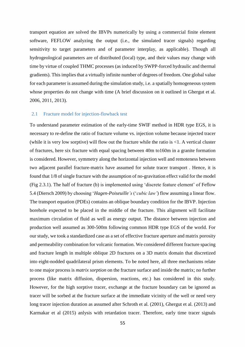
55

transport equation are solved the IBVPs numerically by using a commercial finite element

software, FEFLOW analyzing the output (i.e., the simulated tracer signals) regarding

sensitivity to target parameters and of parameter interplay, as applicable). Though all

hydrogeological parameters are of distributed (local) type, and their values may change with

time by virtue of coupled THMC processes (as induced by SWPP-forced hydraulic and thermal

gradients). This implies that a virtually infinite number of degrees of freedom. One global value

for each parameter is assumed during the simulation study, i.e. a spatially homogeneous system

whose properties do not change with time (A brief discussion on it outlined in Ghergut et al.

2006, 2011, 2013).

2.1 Fracture model for injection-flowback test

To understand parameter estimation of the early-time SWIF method in HDR type EGS, it is

necessary to re-define the ratio of fracture volume vs. injection volume because injected tracer

(while it is very low sorptive) will flow out the fracture while the ratio is <1. A vertical cluster

of fractures, here six fracture with equal spacing between 40m to160m in a granite formation

is considered. However, symmetry along the horizontal injection well and remoteness between

two adjacent parallel fracture-matrix have assumed for solute tracer transport . Hence, it is

found that 1/8 of single fracture with the assumption of no-gravitation effect valid for the model

(Fig 2.3.1). The half of fracture (b) is implemented using ‘discrete feature element’ of Feflow

5.4 (Diersch 2009) by choosing ‘Hagen-Poiseuille’s (‘cubic law’) flow assuming a linear flow.

The transport equation (PDEs) contains an oblique boundary condition for the IBVP. Injection

borehole expected to be placed in the middle of the fracture. This alignment will facilitate

maximum circulation of fluid as well as energy output. The distance between injection and

production well assumed as 300-500m following common HDR type EGS of the world. For

our study, we took a standardized case as a set of effective fracture aperture and matrix porosity

and permeability combination for volcanic formation. We considered different fracture spacing

and fracture length in multiple oblique 2D fractures on a 3D matrix domain that discretized

into eight-nodded quadrilateral prism elements. To be noted here, all three mechanisms relate

to one major process is matrix sorption on the fracture surface and inside the matrix; no further

process (like matrix diffusion, dispersion, reactions, etc.) has considered in this study.

However, for the high sorptive tracer, exchange at the fracture boundary can be ignored as

tracer will be sorbed at the fracture surface at the immediate vicinity of the well or need very

long tracer injection duration as assumed after Schroth et al. (2001), Ghergut et al. (2013) and

Karmakar et al (2015) anlysis with retardation tracer. Therefore, early time tracer signals

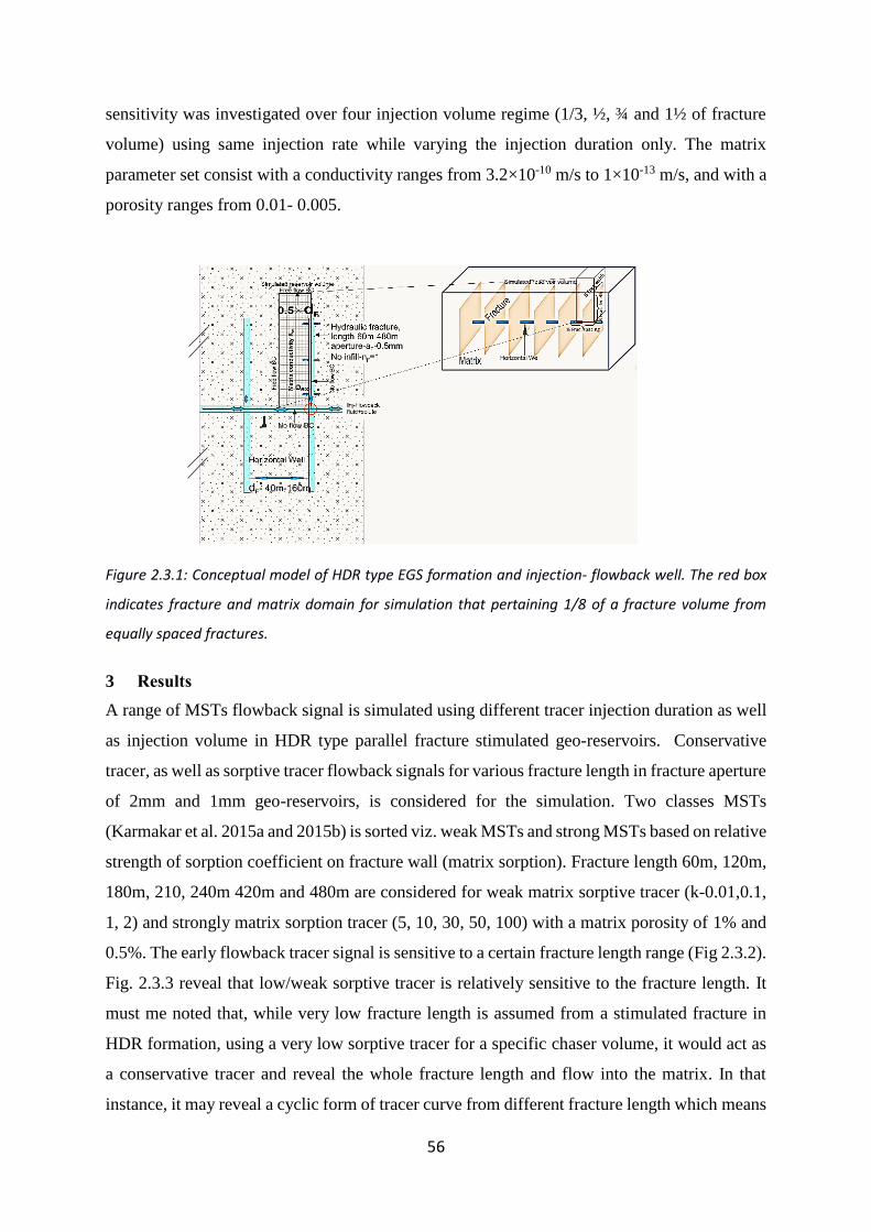
56

sensitivity was investigated over four injection volume regime (1/3, ½, ¾ and 1½ of fracture

volume) using same injection rate while varying the injection duration only. The matrix

parameter set consist with a conductivity ranges from 3.2×10-10 m/s to 1×10-13 m/s, and with a

porosity ranges from 0.01- 0.005.

Figure 2.3.1: Conceptual model of HDR type EGS formation and injection- flowback well. The red box

indicates fracture and matrix domain for simulation that pertaining 1/8 of a fracture volume from

equally spaced fractures.

3 Results

A range of MSTs flowback signal is simulated using different tracer injection duration as well

as injection volume in HDR type parallel fracture stimulated geo-reservoirs. Conservative

tracer, as well as sorptive tracer flowback signals for various fracture length in fracture aperture

of 2mm and 1mm geo-reservoirs, is considered for the simulation. Two classes MSTs

(Karmakar et al. 2015a and 2015b) is sorted viz. weak MSTs and strong MSTs based on relative

strength of sorption coefficient on fracture wall (matrix sorption). Fracture length 60m, 120m,

180m, 210, 240m 420m and 480m are considered for weak matrix sorptive tracer (k-0.01,0.1,

1, 2) and strongly matrix sorption tracer (5, 10, 30, 50, 100) with a matrix porosity of 1% and

0.5%. The early flowback tracer signal is sensitive to a certain fracture length range (Fig 2.3.2).

Fig. 2.3.3 reveal that low/weak sorptive tracer is relatively sensitive to the fracture length. It

must me noted that, while very low fracture length is assumed from a stimulated fracture in

HDR formation, using a very low sorptive tracer for a specific chaser volume, it would act as

a conservative tracer and reveal the whole fracture length and flow into the matrix. In that

instance, it may reveal a cyclic form of tracer curve from different fracture length which means

57

additional ambiguity with the tracer signal, and the clear cut relationship with fracture length

and tracer flowback signal will be broken. It follows the monotonic trend of lower breakthrough

concentration with lower fracture length.

Figure 2.3.2: Weak matrix sorption tracer (MSTs) sensitivity in different fracture length for hydraulically

stimulated fracture in HDR type EGS. It shows that very weak sorptive or conservative tracer R=1-1.5,

matrix porosity 3%, k=0-0.01 is sensitive to the fracture length while a big aperture (1mm-2mm) is

created.

58

Figure 2.3.3: Strong MST (matrix sorption tracer) sensitivity in different fracture length for hydraulically

stimulated fracture in HDR type EGS, matrix porosity 1% for a fracture aperture 2mm. Sensitive sorptive

tracer range is k-0.5-1.5.

0.02

0.04

0.06

0.08

0.1

0.12

0.14

0.49 0.59 0.69 0.79 0.89 0.99 1.09 1.19 1.29 1.39 1.49

Con

cen

trati

on

mg

/l

Time (days) after tracer injection (with flowback starting at 0.3 days)

Ref_fL420m k1E-3_fL420m k0.5_fL420m k1.5_fL420m k5_fL420m

Ref_fL210m k1E-3_fL210m k0.5_fL210m k1.5_fL210m k5_fL210m

Ref_fL60m k1E-3__fL60m k0.5_fL60m k1.5_fL60m k5_fL60m

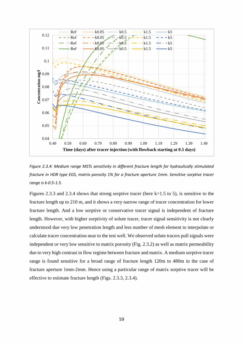
59

Figure 2.3.4: Medium range MSTs sensitivity in different fracture length for hydraulically stimulated

fracture in HDR type EGS, matrix porosity 1% for a fracture aperture 1mm. Sensitive sorptive tracer

range is k-0.5-1.5.

Figures 2.3.3 and 2.3.4 shows that strong sorptive tracer (here k=1.5 to 5), is sensitive to the

fracture length up to 210 m, and it shows a very narrow range of tracer concentration for lower

fracture length. And a low sorptive or conservative tracer signal is independent of fracture

length. However, with higher sorptivity of solute tracer, tracer signal sensitivity is not clearly

understood due very low penetration length and less number of mesh element to interpolate or

calculate tracer concentration near to the test well. We observed solute tracers pull signals were

independent or very low sensitive to matrix porosity (Fig. 2.3.2) as well as matrix permeability

due to very high contrast in flow regime between fracture and matrix. A medium sorptive tracer

range is found sensitive for a broad range of fracture length 120m to 480m in the case of

fracture aperture 1mm-2mm. Hence using a particular range of matrix sorptive tracer will be

effective to estimate fracture length (Figs. 2.3.3, 2.3.4).

0.04

0.05

0.06

0.07

0.08

0.09

0.1

0.11

0.12

0.49 0.59 0.69 0.79 0.89 0.99 1.09 1.19 1.29 1.39 1.49

Co

nce

ntr

ati

on

mg

/l

Time (days) after tracer injection (with flowback starting at 0.5 days)

Ref k0.05 k0.5 k1.5 k5

Ref k0.05 k0.5 k1.5 k5

Ref k0.05 k0.5 k1.5 k5

Ref k0.05 k0.5 k1.5 k5

60

Figure 2.3.5: Effect of higher injection rate/volume, which exceed the fracture volume, for the high MST

(k 5-100, matrix porosity-3%). It shows that strong MSTs show no clear trend with the fracture length.

From the tracer breakthrough, it revealed that fracture length influence tracer breakthrough for

the higher matrix sorptive tracer. To have a consistent tracer signal one should choose very

high sorption tracer or very lower sorption tracer while fracture length is the parameter in

question. However, it is important to note that fracture aperture must know before estimating

the extent of fracture length from this kind of test. The monotonicity of the tracer signal

‘cyclically reversed’ while injection volume is higher than fracture volume (Figs. 2.3.5 and

2.3.6). Hence, during parameter inversion, it needs to be cautious and necessary to consider the

injection volume design to avoid ambiguous fracture length estimation.

4 Sorption tracer selection and sensitivity

Sorptive tracer is particularly useful to determine fracture size in stimulated reservoir both in

sedimentary and crystalline formations which are the particular interest in method development

process in earlier parts (c.f. part 1 and 2) of this chapter. However, it is important to make

available a range of sorption properties would be applied for this kind of test. In that instance,

it observes a decreased sensitivity for fracture thickness with an increase of sorption properties

in case of proppant sorptive tracer in part 1 and part 2. From above sorptive tracer

implementation case in HDR type EGS, it also perceives not a universal range of sorptive tracer

would be effective nor all range sensitive for different stimulated georeservoir formation. In

61

that instance, a medium to higher range sorptive tracer would be particular importance for HDR

application for fracture length as it would not be affected by lower fracture volume. However,

for fracture length estimation should follow after a preliminary evaluation which would

determine the appropriate range of sorption tracer to be used.

Figure 2.3.6: Simulated signals of multiple PST and MST (characterized by different Kd values) during

GPF flowback, at a fixed value of GPF thickness (12mm) and proppant-packing porosity (30%).

0.03

0.05

0.07

0.09

0.11

0.13

0.15

0.17

0.19

0.3 0.4 0.5 0.6 0.7 0.8 0.9 1

Co

nce

ntr

atio

n m

g/L

Time (days) after tracer injection (with flowback starting at 0.3 days)

62

Figure 2.3.7: Simulated signals of multiple PST during GPF flowback, at a different value of GPF and

proppant-packing porosity (30% and 60%).

0.07

0.09

0.11

0.13

0.15

0.17

0.19

0.21

0.3 0.4 0.5 0.6 0.7 0.8 0.9 1

Co

nce

ntr

atio

n m

g/L

Time (days) after tracer injection (with flowback starting at 0.3days)

tF4mm tF4mm

tF8mm tF8mm

tF12mm tF12mm

tF16mm tF16mm

tF20mm tF20mm

tF24mm tF24mm

0.065

0.085

0.105

0.125

0.145

0.165

0.185

0.205

0.3 0.4 0.5 0.6 0.7 0.8 0.9 1

Co

nce

ntr

ati

on

mg

/L

Time (days) after tracer injection (with flowback starting at 0.5 days)

Ref k20 k30 k40 k50 k80 k100

k130 k170 k220 k280 k400 k480

63

Figure 2.3.8: Simulated signals of multiple PST (characterized by different Kd values) during GPF

flowback, at a fixed value of GPF thickness (12mm) and proppant-packing porosity (40%). Signals are

labeled by the retardation factor k (k= Kd × proppant density).

Figure 2.3.9: The injection volume is in the same size or higher that fracture volume for lower

two example fracture length, which break the monotonicity of tracer breakthrough and signal

grows rather reversibly.

5 Discussion and conclusion

The minimum sorptivity (minimum κ value) that required to induce sufficient contrast between

measurable tracer signals for different values of target parameters has discussed in chapeter 2

part 1 (see also in Karmakar et al 2015a). The scheme is: a p% change in a target parameter

value produces c% change in the signal of a conservative tracer, and a s% change in the signal

of a sorptive tracer, s being a function of κ. For PSTs and MSTs based SWIF test study, a lower

sorptive tracer than its minimum necessary is suggested, assuming an increase sensitivity factor

(ratio between sorptive tracer signal changes to conservative tracer signals changes, s/c)

approximately equal to √ (1 + 0.7× sorption coefficient, κ). This empirical relationship delimits

that too much investment on highly sorptive tracer will not affect tracer parameter sensitivity

at same magnitude (Figure 2.3.4 and 2.3.5). One needs to note that the higher the tracer's

retardation, the lower is its fracture invasion, and consequently a poorer capability for

characterizing the fracture as a whole. In principle, this could be compensated by increasing

0.04

0.05

0.06

0.07

0.08

0.09

0.1

0.11

0.12

0.49 0.59 0.69 0.79 0.89 0.99

Co

nce

ntr

atio

n m

g/l

Time (days) after tracer injection (with flowback starting at 0.5 days)

fL_480m_Ref k0.05 k0.5 k1.5 k5fL300m_Ref k0.05 k0.5 k1.5 k5fL210m_Ref k0.05 k0.5 k1.5 k5

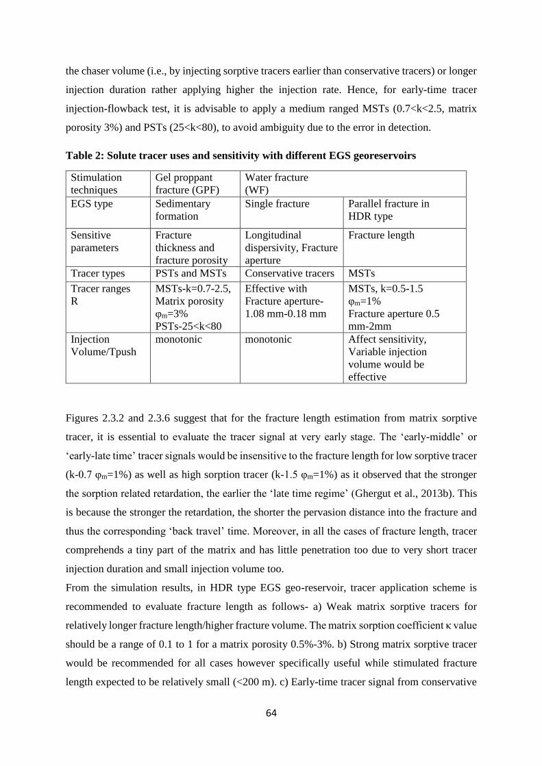
64

the chaser volume (i.e., by injecting sorptive tracers earlier than conservative tracers) or longer

injection duration rather applying higher the injection rate. Hence, for early-time tracer

injection-flowback test, it is advisable to apply a medium ranged MSTs (0.7<k<2.5, matrix

porosity 3%) and PSTs (25<k<80), to avoid ambiguity due to the error in detection.

Table 2: Solute tracer uses and sensitivity with different EGS georeservoirs

Stimulation

techniques

Gel proppant

fracture (GPF)

Water fracture

(WF)

EGS type Sedimentary

formation

Single fracture Parallel fracture in

HDR type

Sensitive

parameters

Fracture

thickness and

fracture porosity

Longitudinal

dispersivity, Fracture

aperture

Fracture length

Tracer types PSTs and MSTs Conservative tracers MSTs

Tracer ranges

R

MSTs-k=0.7-2.5,

Matrix porosity

φm=3%

PSTs-25<k<80

Effective with

Fracture aperture-

1.08 mm-0.18 mm

MSTs, k=0.5-1.5

φm=1%

Fracture aperture 0.5

mm-2mm

Injection

Volume/Tpush

monotonic monotonic Affect sensitivity,

Variable injection

volume would be

effective

Figures 2.3.2 and 2.3.6 suggest that for the fracture length estimation from matrix sorptive

tracer, it is essential to evaluate the tracer signal at very early stage. The ‘early-middle’ or

‘early-late time’ tracer signals would be insensitive to the fracture length for low sorptive tracer

(k-0.7 φm=1%) as well as high sorption tracer (k-1.5 φm=1%) as it observed that the stronger

the sorption related retardation, the earlier the ‘late time regime’ (Ghergut et al., 2013b). This

is because the stronger the retardation, the shorter the pervasion distance into the fracture and

thus the corresponding ‘back travel’ time. Moreover, in all the cases of fracture length, tracer

comprehends a tiny part of the matrix and has little penetration too due to very short tracer

injection duration and small injection volume too.

From the simulation results, in HDR type EGS geo-reservoir, tracer application scheme is

recommended to evaluate fracture length as follows- a) Weak matrix sorptive tracers for

relatively longer fracture length/higher fracture volume. The matrix sorption coefficient κ value

should be a range of 0.1 to 1 for a matrix porosity 0.5%-3%. b) Strong matrix sorptive tracer

would be recommended for all cases however specifically useful while stimulated fracture

length expected to be relatively small (<200 m). c) Early-time tracer signal from conservative

65

solute can determine the aperture of fractures created by a WF treatment. However, the

effectiveness needs to be verified for very thin fractures (<0.2 mm) as suggested in (Karmakar

et al., 2015a and 2015b).

Acknowledgments: The first author gratefully acknowledges continued financial support from

the DAAD (German Academic Exchange Service) to pursue his Ph.D. work. This work also

benefited from long-term financial and technical support granted by the Federal German

Ministry for Economic Affairs and Energy (BMWi) within the project TRENDS (2014-2018,

FKZ 0325515).

References

Breede K, Dzebisashvili K, Liu X, Falcone G, 2013, A Systematic review of enhanced (or

engineered) geothermal systems: past, present and future. Geothermal Energy.

doi:10.1186/2195-9706-1-4.

Diersch, H.-J., G., 2009. FEFLOW 5.4: finite element subsurface flow and transport simulation

system. Reference manual. DHI-WASY Ltd., Berlin, Germany, 292 pp

Jiang F., Chen, Huang, W. Luo L. 2014, A three-dimensional transient model for EGS subsurface

thermo-hydraulic process, Energy 72, 300–310.

Jung R., 2013, EGS — Goodbye or Back to the Future 95, Effective and Sustainable Hydraulic

Fracturing, Dr. Rob Jeffrey (Ed.), ISBN: 978-953-51-1137-5,InTech, DOI: 10.5772/56458.

Available from: http://www.intechopen.com/books/effective-and-sustainable-hydraulic-

fracturing/egs-goodbye-or-back-to-the-future-95.

Ghergut, I., Behrens, H., Sauter, M., 2013a. Can Peclet numbers depend on tracer species? going

beyond SW test insensitivity to advection or equilibrium exchange. In: Proceedings 38th

Workshop on Geothermal Reservoir Engineering, Stanford Univ. (CA), SGP-TR-198, 326-

335.

Ghergut, I., Behrens, H., Sauter, M., 2013b. Single-well tracer push-pull test sensitivity to fracture

aperture and spacing. In: Proceedings 38th Workshop on Geothermal Reservoir Engineering,

Stanford Univ. (CA), SGP-TR-198, 295-308.

Karmakar, S., Ghergut, I., Sauter, M., 2015a, EGS in sedimentary basins: sensitivity of early-

flowback tracer signals to induced-fracture parameters. Energy Procedia 76, 223-229.

Karmakar, S., Ghergut, J., Sauter, M., 2015b, Early-flowback tracer signals for fracture

characterization in an EGS developed in deep crystalline and sedimentary formations: a

parametric study, Geothermics, in press, doi:10.1016/j.geothermics.2015.08.007

Schulte T, Zimmermann G, Vuataz F, Portier S, Tischner T, Junker R, Jatho R, Huenges E 2010,

Enhancing geothermal reservoirs. In: Huenges E (ed) Geothermal Energy Systems:

Exploration, Development, and Utilization. Wiley-VCH, Berlin, pp 173–243

66

CHAPTER 3-PART 1: Single-well tracer injection-flowback test simulation in fractured

georeservoir using finite element code FEFLOW and COMSOL- a benchmark study

Shyamal Karmakar, Sandra Oehlmann, Julia Ghergut, Martin Sauter

Citation:

Karmakar, S., Oehlmann, S., Ghergut, J., Sauter, M., Benchmark study on flow and solute

transport in geological reservoirs, draft paper

Geoscience Centre of the University of Göttingen, Department of Applied Geology,

Goldschmidtstrasse 3, 37077 Göttingen, Germany

*Corresponding author: shyamal.karmakar@geo.uni-goettingen.de

67

Abstract

The single well push-pull tracer simulation study in chapter 2 of this thesis uses a single fracture

model with tetrahedral mesh. The flow is assumed as cubic law for ‘no’ infill fracture (water-

fracture) and Darcy flow for gel-proppant filled fracture in the numerical modeling package

FEFLOW. The simulation results were reproduced in this part thesis using higher temporal and

spatial discretization in FEFLOW. At the same time, the same model was set in COMSOL

Multiphysics, which make uses of fracture and matrix model as a hybrid model of 3D matrix

domain with a lower dimention-2D fracture element. The result was compared qualitatively in

terms of capturing the spikes of injection and flowback in early flow back tracer test. From this

two approaches of simulation, it is revealed that at early times, the numerical dispersion is an

issue for conservative tracer simulation, while it is negligible for sorptive tracers. Moreover,

COMSOLs PDE interface is a useful tool to build and simulate flow and solute transport for a

fracture domain as well.

1 Model concept

This study compares the simulation results of two finite element based modeling software

packages viz. FEFLOW and COMSOL Multiphysics for flow and solute transport for a single

well tracer push-pull test in a single fracture model. The difference between the simulation

results and the computational efficiency between the two numerical simulators are quantified

for single-well tracer push-pull test for multi-tracer use in conjunction with gel-proppant

fracture (GPF) treatments. The numerical model in FEFLOW and COMSOL consider two

simplified fracture models based on lithostratigraphic and hydrogeologic data from the

Geothermal In-Situ Laboratory at Groß-Schönebeck in the NE-German basin (c.f. Karmakar

et al 2015a, 2015b). The commercially available finite-element software FEFLOW 5.4

(Diersch, 2009) and COMSOL Multiphysics 4.4 were used to simulate fluid flow and tracer

transport in fractures resulting from GPF, relying on some simplifying assumptions. The rock

matrix is treated like a single-porosity medium in 3D, whereas vertical planar fractures are

represented by lower-dimensional (2D) so-called 'discrete elements'. Flow and transport in

fracture and matrix compartments are coupled to each other by FEFLOW's special,

computationally efficient approach. Flow within water-fracture type (WF) fractures is assumed

to obey the 'cubic law' (Tsang, 1992); flow within the matrix, as well as within GPF-type

fractures, is assumed as Darcian. Thus, GPF-type fractures are treated almost like an ordinary

porous medium, which (with the exception of solute exchange with the adjacent rock matrix)

68

is similar to the 'push-pull' test situation considered by Schroth et al. (2001). Solute transport

in fractures, and within rock matrix is assumed as advective-dispersive, with a number of

additional processes at fluid-solid interfaces as described below (adsorption-desorption

onto/from matrix rock, or proppant coatings; matrix diffusion). The model has to be 3D because

of its fracture (approximately radial) and matrix (approximately linear) flow and transport

components. The assumption of horizontal and vertical symmetry and neglecting gravity

effects means that it needs to consider only one-quarter of the fracture plane, one-half of the

fracture aperture or thickness and one-eighth of its adjacent matrix block (similar to the model

used by Ghergut et al., 2013b for parallel-fracture systems). The geometry of model

compartments (fracture and matrix block) and the hydrogeological parameter distribution for

the WF and GPF target layers are shown in Fig. 3.1.1. The assumption of isotropic permeability

(described by a single scalar value for each compartment) is rather unrealistic, but it does not

influence the parameter sensitivity behaviour of simulated tracer signals. Further, we assume

isothermal conditions; the hydraulic conductivity values listed in Fig. 3.1.1 corresponds to a

temperature of 120°C, assumed to prevail during tracer injection and early flowback, as a

transient 'equilibrium' between native reservoir conditions (~160°C) and injected fluid

temperature (~15°C).

69

Figure 3.1.1: 3D model domain and hydrogeological parameter distribution. The rectangular mesh

shown here is used in FEFLOW simulation. COMSOL simulation is done in the triangular mesh.

Flow and solute transport model PDE describe for 2D, phreatic, Darcy flow in Diersch (2009)

used in FEFLOW as follows.

𝑆𝑑ℎ

𝑑𝑥− ∇. (𝐾𝐵. (∇ℎ + 𝜃𝑒)) − 𝑄 = 0 … … … … … … … … … … … … … … … … … (1)

In water fracture flow, K evaluated as shown below

𝐻𝑎𝑔𝑒𝑛 𝑃𝑜𝑖𝑠𝑢𝑖𝑙𝑙𝑎𝑒 (𝐶𝑢𝑏𝑖𝑐 𝑙𝑎𝑤), 𝐾 =𝑏3𝜌0𝑔

12𝜇0… … … … … … . . (2)

Here S[L-1] - specific storage, K [LT-1] - Darcy conductivity in fracture or Conductivity as

cubic law fracture , b [L] is the total fracture thickness for gel-proppant fracture or fracture

hydraulic aperture for water-fracture (Tang et al 1992), dynamic viscosity 𝜇0[MLT3], density

of fluid, 𝜌0[ML-3], source or sink of fluid Q [L3T-1].

Injection and flowback Well

Rock matrix ≈3700 element

70

Solute transport in fracture

𝑆𝑑𝑐

𝑑𝑡+ 𝑞. ∇𝑐 − ∇. (𝐵휀𝐷. ∇𝐶) + 𝐵(휀𝑄𝑝 + 𝜗) − 𝑄𝑐 = 0 … … … . . (3)

𝐷𝑖𝑠𝑝𝑒𝑟𝑠𝑖𝑣𝑖𝑡𝑦, 𝐷 = 𝐷𝑑 + 𝐷𝑚

q[𝐿𝑇−1 ]- Darcy velocity vector, 𝜗-degradation or decay, 𝐷𝑑[𝐿𝑇−2 ] -hydrodynamic

dispersivity in fracture, 𝐷𝑚 [L2T-1]- molecular diffusion of solutes

Hydrodynamic dispersion tensor used in FEFLOW according to Bear-Scheidegger dispersion

tensor for matrix and fracture

𝐷𝑚𝑎𝑡𝑟𝑖𝑥 = 𝐷𝑑 + 𝐷𝑚 = 𝐷𝑑 + 𝛽𝑇𝑣 + (𝛽𝐿−𝛽𝑇)𝑞⨂𝑞

|𝑞|… … … . . (4)

𝐷𝑓𝑟𝑎𝑐𝑡𝑢𝑟𝑒 = 𝐷𝑑 + 𝐷𝑚 = 𝐷𝑑 + 𝛽𝐿

𝑞⨂𝑞

|𝑞|… … … . . (5)

Whereas, the dispersion tensor in COMSOL implemented as Burnett and Frind (1987) read as

𝐷𝑓𝑟𝑎𝑐𝑡𝑢𝑟𝑒 = 𝐷𝑑 + 𝐷𝑚 = 𝐷𝑑 + (𝛽𝐿−𝛽𝑇)𝑞⨂𝑞

|𝑞|… … … . (6)

A derivative of retardation coefficient, R also used for the background solute retardation which

is not relevant for this study as initial concentration C0 assumed both in fracture and matrix and

R is defined as

𝑅 = 1 + 𝜌 × 𝐾𝑑 ×1−𝑛

𝑛= 1 + κ ×

1−n

n… … … . . (7)

Where, as 𝜅 = 𝜌 × 𝐾𝑑, 𝜅 is the sorption coefficient, 𝐾𝑑[ ]-sorption distribution coefficient

(slope of linear segment of adsorption isotherm, Freeze and Cherry, 1979), n [ ] –is the porosity

medium (for matrix sorptive tracer, matrix porosity and for proppant sorptive tracer, proppant

packing), 𝜌[𝑀𝐿−3]- intrinsic the density of solid-phase material (either rock or proppants).

The retardation factor R is not an intrinsic tracer property, but it also depends on the porosity

of the transport medium; as equation 7 shows R-values cannot be varied independently of

porosity.

The exchange between fracture and matrix implemented in COMSOL as

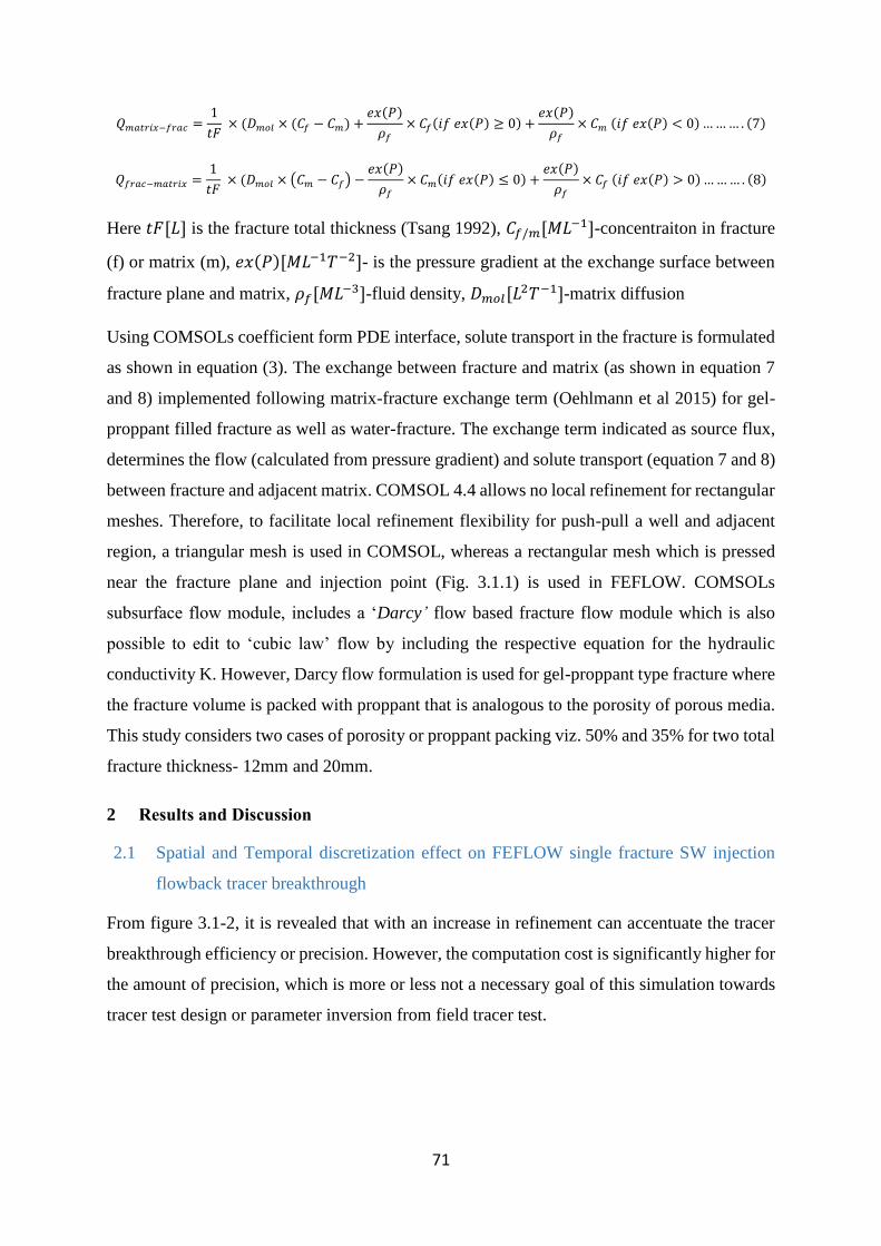
71

𝑄𝑚𝑎𝑡𝑟𝑖𝑥−𝑓𝑟𝑎𝑐 =1

𝑡𝐹 × (𝐷𝑚𝑜𝑙 × (𝐶𝑓 − 𝐶𝑚) +

𝑒𝑥(𝑃)

𝜌𝑓

× 𝐶𝑓(𝑖𝑓 𝑒𝑥(𝑃) ≥ 0) +𝑒𝑥(𝑃)

𝜌𝑓

× 𝐶𝑚 (𝑖𝑓 𝑒𝑥(𝑃) < 0) … … … . (7)

𝑄𝑓𝑟𝑎𝑐−𝑚𝑎𝑡𝑟𝑖𝑥 =1

𝑡𝐹 × (𝐷𝑚𝑜𝑙 × (𝐶𝑚 − 𝐶𝑓) −

𝑒𝑥(𝑃)

𝜌𝑓

× 𝐶𝑚(𝑖𝑓 𝑒𝑥(𝑃) ≤ 0) +𝑒𝑥(𝑃)

𝜌𝑓

× 𝐶𝑓 (𝑖𝑓 𝑒𝑥(𝑃) > 0) … … … . (8)

Here 𝑡𝐹[𝐿] is the fracture total thickness (Tsang 1992), 𝐶𝑓/𝑚[𝑀𝐿−1]-concentraiton in fracture

(f) or matrix (m), 𝑒𝑥(𝑃)[𝑀𝐿−1𝑇−2]- is the pressure gradient at the exchange surface between

fracture plane and matrix, 𝜌𝑓[𝑀𝐿−3]-fluid density, 𝐷𝑚𝑜𝑙[𝐿2𝑇−1]-matrix diffusion

Using COMSOLs coefficient form PDE interface, solute transport in the fracture is formulated

as shown in equation (3). The exchange between fracture and matrix (as shown in equation 7

and 8) implemented following matrix-fracture exchange term (Oehlmann et al 2015) for gel-

proppant filled fracture as well as water-fracture. The exchange term indicated as source flux,

determines the flow (calculated from pressure gradient) and solute transport (equation 7 and 8)

between fracture and adjacent matrix. COMSOL 4.4 allows no local refinement for rectangular

meshes. Therefore, to facilitate local refinement flexibility for push-pull a well and adjacent

region, a triangular mesh is used in COMSOL, whereas a rectangular mesh which is pressed

near the fracture plane and injection point (Fig. 3.1.1) is used in FEFLOW. COMSOLs

subsurface flow module, includes a ‘Darcy’ flow based fracture flow module which is also

possible to edit to ‘cubic law’ flow by including the respective equation for the hydraulic

conductivity K. However, Darcy flow formulation is used for gel-proppant type fracture where

the fracture volume is packed with proppant that is analogous to the porosity of porous media.

This study considers two cases of porosity or proppant packing viz. 50% and 35% for two total

fracture thickness- 12mm and 20mm.

2 Results and Discussion

2.1 Spatial and Temporal discretization effect on FEFLOW single fracture SW injection

flowback tracer breakthrough

From figure 3.1-2, it is revealed that with an increase in refinement can accentuate the tracer

breakthrough efficiency or precision. However, the computation cost is significantly higher for

the amount of precision, which is more or less not a necessary goal of this simulation towards

tracer test design or parameter inversion from field tracer test.

72

Figure 3.1.2: Spatial and temporal discretization effect on FEFLOW numerical solution single fracture

tracer flowback concentrations.

The dispersion in COMSOL is implemented as Burnett and Frind (1987) tensor. The

dispersivity tensor for isotropic porous medium can be defined by two constants—the

longitudinal dispersivity of the medium, αL, and the transverse dispersivity of the medium, αT

(Scheidegger 1961). However, in anisotropic media, the number of independent dispersivity

values increases (Bear and Cheng 2010). Although conventional theory holds that αL is an

intrinsic property of the aquifer, it is found in practice to be dependent on and proportional to

the scale of the measurement. Most reported values of αL fall in a range from 0.01 to 1.0 times

the scale of the measurement, although the ratio of αL to the scale of measurement tends to

decrease at larger scales (Anderson 1984; Gelhar et al. 1992). Field- scale dispersion (macro-

dispersion) results primarily from large-scale spatial variations in hydraulic properties (and

hence in velocity). Yet one can often adequately calibrate a groundwater-flow model to

observed heads using a relatively coarse grid and relatively uniform hydraulic properties that

do not represent heterogeneities that affect transport. If that is the framework for the transport

model, calibrations will likely lead to erroneously large values of dispersivity (e.g., Davis

1986). Similarly, representing a transient flow field by a mean steady-state flow field, as is

commonly done, inherently ignores some of the variability in velocity and must be

0.03

0.04

0.05

0.06

0.07

0.08

0.09

0.1

0.11

0.12

0.5 0.6 0.7 0.8 0.9 1 1.1 1.2

Co

nce

ntr

atio

n m

g/l

Time (Days) after flowback started

Ref_TS1E-2_1X 100P_TS1E-2_1X 100M_TS1E-2_1XRef_TS1E-3_2X 100P_TS1E-3_2X 100M_TS1E-3_2XRef_TS5E-3_8X 100P_TS5E-3_8X 100M_TS5E-3_8XRef_TS5E-4_16X 100P_TS5E-4_16X 100M_TS5E-4_16X

73

compensated for by using increased values of dispersivity (primarily transverse dispersivity)

(Goode and Konikow 1990). Moreover, it is important to note that the sorptive tracer either

proppant or matrix sorptive tracer showed similar concentration breakthrough with small

difference 2E-3 which reveals a higher effect of sorption on tracer breakthrough than

dispersion. Hence, to avoid or reduce the dispersion impact on the single well tracer test, a

sorptive tracer would be an ideal choice for parameter estimation if sufficient sensitivity regime

exists with the target parameter.

2.2 Tracer flowback signals in COMSOL and FEFLOW from gel-proppant fracture and

water fracture, simulation concept and limitation

Figure 3.1.3: Tracer spreading inside the fracture and matrix during at 1 day while flowback start at

0.5 days for conservative tracer-3a (from left), low matrix sorptive tracer-3b and high MSTs- 3c

74

Figure 3.1.4a-b: Tracer concentration (a) and Hydraulic head (b) from different fracture porosity for

injection-flowback benchmark study in single fracture-matrix domain using PDEs module in software

package COMSOL Multiphysics.

Hydraulic head at the injection-flowback well showed an equal head over the whole test

duration (Figure 3.1.4b). Moreover, the tracer concentration from different fracture porosity

shows similar result as seen in FEFLOW simulation (Figure 3.1.4b). With the same model

setup, fracture thickness result shows very different head and tracer flowback concentration

than FEFLOW simulation result for same fracture and matrix parameters. This result signifies

that the exchange term used in COMSOL to transfer across the fracture to matrix domain need

to be review. The problem may be arising from the pressure/flow exchange term as the

hydraulic head show greater anomalies (c.f. Appendix 2a).

The exchange term that implemented for fluid and solute exchange between fracture and matrix

estimated as less amount of solute intrude into the matrix in COMSOL than that computed in

FEFLOW, where the fracture is implemented as a discrete feature. The exchange term in

COMSOL is explicitly formulated as describe in Oehlmann et al. (2015) considering the 2D

exchange surface with the matrix. However, the simulation not comparable with the pressure

head (shows 5 times higher) during injection and flowback simulation as well as flowback

concentration is not relevant to compare. A major challenge with this translation of fractured

geo-reservoir simulation has lied with the matrix and fracture exchange term, to include

appropriate format fracture thickness inclusion as well as exchange pressure. However, the

75

lesson from this fractured geo-reservoir simulation is extremely valuable for future code

development for fractured geo-reservoir tracer flowback simulation as well as a close-form

analytical solution development for solute transport.

References

Anderson, M.A. 1984. Movement of contaminants in ground- water: Groundwater transport—

Advection and dispersion. In: Groundwater Contamination, 37–45. Washington, DC: National

Academy Press.

Burnett, R.D. and Frind E.O., 1987, Simulation of contaminant transport in three dimensions. 2.

Dimensionality effects, Water Resource Research., 23, 695-705.

Diersch, H.-J., G., 2009. FEFLOW 5.4: finite element subsurface flow and transport simulation

system. Reference manual. DHI-WASY Ltd., Berlin, Germany, 292 pp

Oehlmann, S., Geyer, T., Licha, T., and Birk, S., 2013. Influence of aquifer heterogeneity on karst

hydraulics and catchment delineation employing distributive modeling approaches. Hydrology

and Earth System Sciences 17, 4729-4742, doi:10.5194/hess-17-4729-2013.

Oehlmann, S., Geyer, T., Licha, T., and Sauter, M., 2015. Reducing the ambiguity of karst aquifer

models by pattern matching of flow and transport on catchment scale. Hydrology and Earth

System Sciences 19, 893–912, doi:10.5194/hess-19-893-2015.

Scheidegger A.E. 1961. General theory of dispersion in porous media. Journal of Geophysical

Research 66, no. 10: 3273–3278.

Konikow, L.F. 2011, The Secret to Successful Solute-Transport Modeling, Ground Water 49(2),

144–159.

Konikow, L.F., W.E. Sanford, and P.J. Campbell. 1997. Constant-concentration boundary

condition: Lessons from the HYDROCOIN variable-density benchmark problem. Water

Resources Research 33, no. 10: 2253–2261.

Gelhar, L.W., C. Welty, and K.R. Rehfeldt. 1992. A critical review of data on field-scale dispersion

in aquifers. Water Resources Research 28, no. 7: 1955–1974.

Gelhar, L.W., and C.L. Axness. 1983. Three-dimensional analysis of macrodispersion in a stratified

aquifer. Water Resources Research.

Tsang, Y.W., 1992. Usage of 'Equivalent Apertures' for Rock Fractures as Derived From Hydraulic

and Tracer Tests. Water Resour. Res. 28(5), 1451-1455.

76

CHAPTER 3-Part 2: A set of benchmark studies on flow and solute transport in

geological reservoirs

Shyamal Karmakar, Alexandru Tatomir , Sandra Oehlmann, Markus Giese, Martin Sauter

Citation:

Karmakar, S., Tatomir, A., Oehlmann, S., Giese, M., Sauter, M., 2016, A set of benchmark

studies on flow and solute transport in geological reservoirs, Prepared for the journal

Computational Geoscience and Modeling, 2016

Geoscience Centre of the University of Göttingen, Department of Applied Geology,

Goldschmidtstraße 3, 37077 Göttingen, Germany

*Corresponding author: shyamal.karmakar@geo.uni-goettingen.de

77

Abstract

Modeling groundwater flow and solute transport are important for a set of engineering and

hydrogeological applications. One of the most common examples is the designing of tracer

tests used for the characterization of geological reservoirs. The quality of the prediction to be

made with a numerical simulator is highly dependent on the quality of the numerical simulator

itself. Besides the accuracy of the results, aspects like financial costs of the simulation software

and the computer resources needed for simulation have to be taken into account. This study

gives an evaluation of different numerical models/approaches and outlines the advantages and

disadvantages of several numerical solution software packages in terms of solution

predictability, temporal control, and computational efficiency. A set of well-established

software frequently used for modeling flow and transport in geological reservoirs is tested and

compared (MODFLOW/MT3DMS, FEFLOW, COMSOL Multiphysics and DuMux). Those

modeling tools are based on different numerical discretization schemes i.e. finite differences,

finite volumes and finite element methods. The influence of dispersivity, which is directly

related to the numerical modeling, is investigated in parametric studies and results are

compared with analytical approximations. At the same time, relative errors are studied in a

complex field scale example. From this comparative study, it is revealed that under forced

gradient conditions, finite element codes COMSOL and FEFLOW show a higher accuracy with

respect to the analytical approximation for a certain range of dispersivity than DuMux and

MODFLOW/MT3DMS. Comparing simulation time and code parallelization, FEFLOW

performs better than COMSOL. Overall computational time is lowest for finite difference

software MODFLOW/MT3DMS for a small number of mesh elements (~ less than 12800

elements). For large meshes (>128000 elements), finite element software FEFFLOW performs

faster.

1 Introduction

Benchmarking numerical software for fluid flow and solute transport is a state of the art for

decades. Usually, the developers of a software or analytical approximation verify and optimize

their software or codes through conducting a number of forward simulations for a set of

benchmark problems (e.g. HYDROCOIN, Ogata and Bank, 1961, Zheng and Wang 1999,

Diersch 2009, Kolditz 2016). These benchmarks show the accuracy of the numerical solver

with respect to established analytical or approximate solutions. Most of the software’s user

manuals or reference books (e.g. Diersch, 2013, Zheng and Wang, 1999) include example

applications with benchmark problems showing solution accuracy. Further, some developers

78

present and document user’s experiences on their web-pages or in newsletters. There are also

independent studies such as ‘software spotlight’ in the journal ‘Groundwater’, which discuss

individual software installation, implementation of parameters and boundary condition as well

as performances.

Some benchmarks also include software applicability, e.g. solution efficiency, code

parallelization, resource uses or user friendliness. However, these usually refer only to a single

software package and do not allow for comparison between different numerical codes (e.g.,

Class et al 2009). The benchmark simulations given for the different software packages differ

in the problem setup, e.g. in terms of spatial discretization or mesh type, making it difficult to

compare them. Further, aspects like financial cost are not taken into account. This makes it

difficult for the user to decide on the numerical simulator to be used for a certain problem.

The partial differential equations describing groundwater flow and transport can be solved

mathematically using either analytical solutions or numerical solutions. For most field

problems, the mathematical benefits of obtaining an analytical solution are probably

outweighed by the errors introduced by the simplifying assumptions for the complex field

environment that are required to apply the analytical model. In most aquifers the most

important parameter controlling transport is hydraulic conductivity, through its control of

velocity (equation 2). Consequently, solute spreading will be represented by local differences

in advection, so uncertainty in estimating dispersivity and conceptual flaws in the mathematical

representation of the dispersion process will matter less. The dispersivity parameter is

conceived as a measurable physical parameter that primarily reflects the nature of the

heterogeneity in the system, where dispersivity determines the spreading of solutes in the

porous media. However, numerical dispersion occurs during the numerical solution process

due to spatial and temporal discretization. From the numerical solution breakthrough curves, it

is difficult to distinguish these two types of dispersion. Therefore, the sensitivity of numerical

simulation results with the dispersivity values is studied in three benchmark problems.

In this study, different factors for selecting software are considered. FEFLOW and

MODFLOW/MT3DMS are the most common ones highly dedicated to porous media flow and

solute transport. They are compared with COMSOL Multiphysics and DuMux, which were

developed for extended applications but are also applicable for single phase flow and solute

transport in porous media. MODFLOW is based on the finite difference method for spatial

discretization, which is the most popular and pioneered in numerical simulations of fluid flow.

79

FEFLOW and COMSOL Multiphysics both are based on the finite element method, which

allows for more flexible meshing. Lastly, DuMux is an academic free open source software

based on the finite volume method dedicated to multiphase flow and transport problems. The

software packages are compared with respect to solution accuracy, efficiency, i.e. time and

computer resources needed, user friendliness and financial cost.

2 Methodology

2.1 Mathematical model

The flow equations that are solved in the analytical approximation and the numerical software

are:

𝑆0

𝜕𝑝

𝜕𝑡+ ∇ ⋅ 𝑞𝑖 − 𝑄𝑝 = 0 … … … … … … … … … … … … … … … … . . (1)

𝑞𝑖 = − {𝜌𝐊

𝜇(𝑔𝑟𝑎𝑑 𝑝 − 𝜌𝐠)} … … … … … … … … … … … … … … … . (2)

𝑆0 [L-1] is the storage term, 𝐊 [L2] is the intrinsic permeability, p [ML-1T-2] is pressure, 𝑞𝑖

[LT-1] is the Darcy velocity vector, 𝑥𝑖 is the spatial discretization vector, 𝑄𝑝 the source or sink

for fluid, 𝜇 [ML-1T-1] the dynamic viscosity, 𝜌 [ML-3] the density of fluid, and g [LT-2] the

acceleration due to gravity.

Transport is described by an advection-dispersion equation of divergent form that is solved in

the numerical software as follows:

𝜕𝐶

𝜕𝑡− ∇ ⋅ {𝑣𝐶 + 𝐷𝑖𝑗𝑔𝑟𝑎𝑑𝐶} + 𝑅

𝜕

𝜕𝑡(𝑅𝐶) + ∇𝑞𝐶 − ∇(𝜙𝐷𝑖𝑗∇C) − 𝑄𝑐 − 𝑅𝑘 = 0 … … … (3)

R [] is the retardation, 𝑞𝑖 [LT-1] is the Darcy velocity vector, 𝑄𝑐 [ML-2T-1] the source or sink

for solute, 𝑅𝑘 [ML-2T-1] reaction rate, 𝐷𝑖𝑗 -[L] dispersion vector, C[ML-3] volumetric

concentration.

In case of radial symmetry (for problem 2, 2D) the transport equation (after Schroth et al 2001)

can be written as

80

𝜕𝐶

𝜕𝑡+

𝜌𝑏

𝑛

𝜕𝑆

𝜕𝑡 𝑥− 𝐷𝐿

𝜕2𝐶

𝜕𝑟2+ 𝑞𝑖

𝜕𝐶

𝜕𝑟+ 𝜆𝐶 = 0 … … … (4)

Here C [ML-3] – volumetric concentration, 𝜌𝑏 [ML-3] -density of solid in porous media, n-

porosity, S -storage coefficient, 𝐷𝐿 -[L] longitudinal dispersion, and r the distance as radial co-

ordinate from injection well, 𝜆 [ML-3 T-1]- degradation or decay rate of the solute and v [LT-

1]- the Darcy velocity. In an REV only one velocity exists in time and space, therefore, velocity

fluctuations within the REV are neglected. They are taken into account within the transport

equation by the concept of mechanical dispersion.

The numerical simulators results are compared with the analytical solution for the 1D and 2D

problems that are described in the section below.

The analytical solution for the 1D problem was given by Ogata and Banks (1961),

𝑐(𝑥, 𝑡) =1

2{𝑒𝑟𝑓𝑐 [

𝑥 − 𝑣𝑡

2√𝐷𝐿𝑡] + 𝑒𝑥𝑝 [

𝑣𝑥

𝐷𝐿𝑡] . 𝑒𝑟𝑓𝑐 [

𝑥 + 𝑣𝑡

2√𝐷𝐿𝑡] … … … … … . (5)

The analytical solution for the 2D problem was given by Gelhar and Collins (1971), which was

adapted and modified after Schroth et al (2001) as follow

𝐶

𝐶0=

1

2𝑒𝑟𝑓𝑐 [

(𝑟2−𝑟𝑖𝑛𝑗2 )

√16

3𝛼𝐿 𝑟𝑖𝑛𝑗

3

], where 𝑟𝑖𝑛𝑗 = √𝑄𝑡

𝜋𝑛𝑅………… (6)

Where, v [LT-1]- the Darcy velocity, Q [L3T-1]- the volumetric flow rate, rinj [L] radial distance

that the solute travels during injection, r [L] radial distance of the observation point from the

injection well, 𝐷𝐿 -[L] longitudinal dispersion, 𝛼𝐿 [L] longitudinal dispersivity, Q [L3T-1 ]

injection rate, R [] retardation and n [] porosity. For conservative tracer, R [] is equal to 1.

2.2 Problem definition

Three benchmark problems with gradually increasing geometrical complexity (i.e., 1D, 2D,

and 3D) are defined for this study. A brief description of the problems is given, including the

model geometry, input parameters, boundary conditions and simulation period, in the

subsection below. The structured grid was chosen from the different mesh types available in

the participating software packages, to keep the degrees of freedom to be solved by the

simulators identical. Problem definition for 1D, 2D and 3D were formulated and solved for

flow and solute transport. The computational performance of the different simulators was

81

studied for the 2D and 3D problem cases. For 1D simulation time was relatively very short and

did not vary significantly among the simulators.

2.2.1 Problem 1: 1D - Solute tracer transport for steady state flow with a forced head

gradient in a homogenous aquifer

This benchmark problem and the analytical solution were formulated by Ogata and Banks

(1961). The model domain is defined by a hydraulic head gradient where a constant

concentration source of conservative solute is present at the higher head boundary (left side)

and advective flow carries the solute to the observation point (Figure 3.2.1). Flow and solute

transport are simulated for a 100m long column with a constant head gradient of 0.02 for a

homogenous and isotropic porous medium pertaining a conductivity of 1×10-4 m/s and 25%

porosity. The simulation period is 200 days. The time step is set as one day (maximum time

step size) and the domain is discretized using a mesh size 1m. The observation point is located

at a distance of 50m from the point fixed concentration solute source. For the sensitivity study,

different dispersivity values are simulated.

Figure 3.2.1: Problem 1: 1D model domain assuming a free flow boundary at right end and higher

gradient at left end with a constant point contaminant source.

2.2.2 Problem 2: 2D-Solute transport in a confined homogenous aquifer from a forced

gradient point source

The benchmark problem considered in this section includes the concentration change at an

observation well during injection at a fully penetrating well in a confined aquifer. Constant

solute concentration, Co, is assumed at the injection well. Moreover, constant head boundaries

are imposed at the other three sides of the domain assuming that it would impose a ‘free

outflow’ boundary during the simulation period. Simulation period is 200 days. The time step

is set as one day (maximum time step size). Storage is set to zero so that steady state flow

conditions are achieved instantaneously after the injection. Since a symmetric radial flow and

transport behavior is expected for the stated model set up, the numerical models that are set up

study only half of the domain assuming symmetry at the middle of the domain at the injection

point.

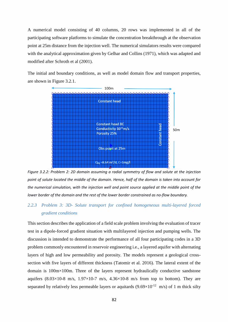
82

A numerical model consisting of 40 columns, 20 rows was implemented in all of the

participating software platforms to simulate the concentration breakthrough at the observation

point at 25m distance from the injection well. The numerical simulators results were compared

with the analytical approximation given by Gelhar and Collins (1971), which was adapted and

modified after Schroth et al (2001).

The initial and boundary conditions, as well as model domain flow and transport properties,

are shown in Figure 3.2.1.

Figure 3.2.2: Problem 2: 2D domain assuming a radial symmetry of flow and solute at the injection

point of solute located the middle of the domain. Hence, half of the domain is taken into account for

the numerical simulation, with the injection well and point source applied at the middle point of the

lower border of the domain and the rest of the lower border constrained as no-flow boundary.

2.2.3 Problem 3: 3D- Solute transport for confined homogeneous multi-layered forced

gradient conditions

This section describes the application of a field scale problem involving the evaluation of tracer

test in a dipole-forced gradient situation with multilayered injection and pumping wells. The

discussion is intended to demonstrate the performance of all four participating codes in a 3D

problem commonly encountered in reservoir engineering i.e., a layered aquifer with alternating

layers of high and low permeability and porosity. The models represent a geological cross-

section with five layers of different thickness (Tatomir et al. 2016). The lateral extent of the

domain is 100m×100m. Three of the layers represent hydraulically conductive sandstone

aquifers (8.03×10-8 m/s, 1.97×10-7 m/s, 4.36×10-8 m/s from top to bottom). They are

separated by relatively less permeable layers or aquitards (9.69×10-12 m/s) of 1 m thick silty

83

clay lenses. The geologic setting of the study site is illustrated in Figure 3.2.3. Thick clay lenses

are also assumed above and beneath the modeled formation. Those layers are assumed to be

impermeable; hence, they are represented by ‘no flow’ type boundaries on top and bottom of

the model domain. The porosity values 14.5%, 16.3% and 13.3% for the permeable sandstone

and 3.9% for the aquitards (Figure 3.2.3) are used. Injection and pumping wells are imposed in

the three conductive layers and each layer is discretized with a uniform thickness of 0.5m. For

the numerical simulation, symmetry is assumed and only half of the domain is modeled. The

model is discretized with a square mesh of 2.5m. The injection rate and pumping rate is 0.432

m3/day at each point (a sum of 8.64 m3/day) as shown in Figure 3.2-3. The time-concentration

data from these simulation results are compared against MODFLOW/MT3DMS data.

Simulation period is 200 days. The time step is set as 0.5 days (maximum time step size). As

the time stepping was found different in different simulation packages, simulation result

efficiency comparisons are done using ‘cubic interpolation’ (a third-degree polynomial)

method in Matlab (http://www.mathworks.com/) to interpolate the data and calculate the

RMSE between the curves.

Figure 3.2- 3: 3D model domain, showing the rectangular mesh and the permeability and porosity

distribution over the layers. Left side points: injection points; right side points: pumping well.

3 Benchmarking simulators

Parametric studies on dispersivity and permeability are investigated for the 3D problem. At

the same time, computational efficiency of different software packages is tested on a Linux

84

platform 4-core 2.32GHz processor CPU with 8 GB RAM memory computer. Among the

participating software, parallel computing for both flow and solute transport modules is only

supported in COMSOL and FEFLOW. Therefore, for these two software packages,

computational performance is studied for both single core and multi-core computing.

3.1 MODFLOW/MT3DMS

MODFLOW is a finite difference method based software which is commonly applied over

decades for fluid flow and solute transport (Harbaugh et al. 2000). As an open source software

distributed by US Geological Survey (USGS) it is freely available but also modified and

revised commercial generic versions such as Visual MODFLOW, PMWIN and GMS are used.

The USGS also provides a pre- and post-processing GUI called ModelMuse, which is also

freely available. For the following analysis, ModelMuse GUI has used for model building and

simulation result visualization. The finite difference based space and time discretization

method is its major advantages which can be expected to cost relatively low memory and

simulation time. The Flow Model Interface Package of MT3DMS reads the saturated thickness,

fluxes across cell interfaces in all directions, locations and flow rates of the various sources

and sinks from an unformatted flow-transport link file saved by a flow model used in

conjunction with the MT3DMS transport model. If the flow model, MODFLOW, is used for

flow simulation, a package named LKMT3 (where 3 denotes the version number) in addition

to MODFLOW is included with the MT3DMS distribution files. For this flow simulation study,

the preconditioned conjugated gradient solver (PCG) in MODFLOW with layer centered grid

and generalized conjugate gradient solver (GCG) in MT3DMS for solute transport are used

using the TVD method (a third order total-variation-diminishing (TVD) scheme for solving the

advection term).

3.2 FEFLOW 6.0

FEFLOW (Finite Element subsurface FLOW and transport system) is an interactive

groundwater modeling software for 2D and 3D fully coupled or uncoupled, thermo-hydro-

chemical (THC) processes in saturated or variably saturated systems. The reactive multi-

species transport can be modeled in subsurface water environments with or without one or

multiple free surfaces. The option to use and develop user-specific plugins via the

programming interface (Interface Manager IFM) allows the addition of external code or even

external programs to FEFLOW. For example, by adding the newly developed mechanical plug-

in it becomes a THMC simulator. It is endowed with a user-friendly model builder interface.

85

Besides the parallelized (OpenMP) computational core, it has also powerful pre- and post-

processing capabilities, including 2D and 3D GIS data, to name some. FEFLOW is available

for WINDOWS systems as well as for different Linux distributions. The current version,

FEFLOW 7.0, which takes over the classic version FEFLOW 6.0, includes a few new features

such as multi-layer wells (would be useful for multilayered-well implementation) with a new

GUI and parameter visualization. However, for this study, FEFLOW 6.0 is used which is the

transitional package that contains both standard new interface as well as ‘classic interface’.

Additional information about FEFLOW is available at http://www.mike-wasy.com. The 3D

multilayered well georeservoir simulation in this benchmark study uses well boundary

conditions that do not act as multilayer wells. Instead, separate well BC for each layer is

introduced.

3.3 COMSOL Multiphysics 4.4

COMSOL Multiphysics (formerly known as FEMLAB) is a finite element software for

numerical simulations of various physical applications. It is mainly employed for technical

applications, but also receives increasing attention for environmental issues during recent years

(e.g. Joodi et al. 2010, Jin et al. 2014, Oehlmann et al. 2013, 2015). In addition to a number of

available interfaces for standard applications, e.g. flow in porous media, COMSOL offers the

possibility to implement individual Partial Differential Equations without needing access to the

source code. This makes COMSOL highly flexible. The software focuses on the

interconnection of different physical processes allowing for multiphysical and

multidimensional couplings. COMSOL can be purchased for Windows, Mac, Linux or UNIX

systems. It offers a number of direct and iterative solvers to choose from for the various

applications. Interfaces to external software, e.g. MathWorks MATLAB

(http://www.mathworks.com/) allow for easy transfer of model results and geometries.

However, limited pre- and post-processing possibilities are also available in COMSOL itself.

The Subsurface Flow Module, which is used in this study, offers standard equations for flow

and transport in saturated and unsaturated porous media. Flow and transport are treated by

separate interfaces. The groundwater flow velocities derived by the flow interface can directly

be used as input for the transport interface. The equations can then either be solved

simultaneously or step-wise reducing simulation time. For this study, the preconditioned

conjugated gradient (PCG) solver is used since this is also the standard solver in FEFLOW.

86

3.4 DuMux

The one phase flow two component transport numerical model, 1p2c, implemented in DuMux

(Flemisch, et al 2011) is used. The free and open source academic numerical model is available

to download at www.dumux.org from a series of ready-to-use models. The Department of

Hydromechanics and Modeling of Hydrosystems, University of Stuttgart, in-house simulator

DuMux is a multi-scale, multiphysics toolbox for the simulation of flow and transport processes

in porous media. The toolbox is based on the Distributed and Unified Numerics Environment

(DUNE) (Bastian et al 2008a, b). DuMux comes in the form of an additional module and inherits

functionality from all available DUNE modules. Its main intention is to provide a framework

for easy and efficient implementation of models for porous media flow problems, ranging from

problem formulation, selection of spatial and temporal discretization schemes and non-linear

solvers, up to general concepts for model coupling. For the space discretization, a BOX scheme

is used, while the time integration is performed via a standard implicit Euler scheme. A

Newton–Raphson method with an adaptive time step selection solves the non-linear equations

in each time step.

4 Result

The results of the benchmark problems are described in the following sections.

4.1 Problem 1: 1D – Solute transport in a homogeneous aquifer with a natural gradient

The analytical solution for concentration breakthrough at 50 m distance from a point source

and the numerical solution simulated for same conditions are presented in Figure 4 for two

dispersivity cases viz. 0.7 m and 5 m. The two distinct sets of curves for different dispersivity

value revealed that all participating simulators, as well as the analytical solution, are sensitive

to this important hydrogeological parameter. Hereby, the dispersivity of 5 m is used as a

standard scenario for the observation at 25m from injection point for 2D and 3D case. Since, it

represents a median value that falls within a range from 0.01 to 1 times ‘scale of measurement’

that can encounter in the field (Anderson 1984; Gelhar et al. 1992). For this value, the accuracy

of all numerical simulators on the analytical solution (after Ogata and Bank, 1961) was judged

to be good with an RMSE of less than 0.1 mg/l (10% of C0). Figure 3.2.5 gives the RMSE of

the breakthrough curves at the observation well predicted by the participating software

packages in problem 1 for different dispersivity value.

87

Figure 3.2.4: Problem 1, tracer breakthrough from various solvers with dispersivities 5m and 0.7m.

Figure 3.2.5: The relative difference between the numerical and analytical solutions within the

simulated range of dispersivity values.

The lower dispersivity case, here 0.7 m, shows higher differences between the simulated

breakthrough curves. This effect is especially pronounced for DuMux. It is important to note

0

0.2

0.4

0.6

0.8

1

20 40 60 80 100 120 140

Co

nce

ntr

atio

n m

g/l

Time (Days)

FEFLOW_dL0.7 FEFLOW_dL5

COMSOL_dL0.7 COMSOL_dL5

MF/MT3DMS_dL0.7 MF/MT3DMS_dL5

DUMUX_dL0.7 DUMUX_dL5

Analytical_dL0.7 Analytical_dL5

0

0.01

0.02

0.03

0.04

0.05

0.06

0.07

0.08

0.09

0.1

0.1 0.3 0.5 0.7 1 3 5 7 10

RM

SE (

mg/

l) f

rom

An

alyt

ical

So

luti

on

Dispersivity (m)

MF/MT3DMS

FEFLOW

COMSOL

DuMux

88

that the RMSE significantly decreases at higher dispersivity values (c.f. Fig. 3.2.4 and Fig

3.2.5). DuMux shows high RMSE values for dispersivity of less than 3 m while the errors are

similar to the other software packages for higher dispersivity values. However, all errors

(maximum value) lay in a range of 2-8% of C0, being well beneath the threshold of 10% of

peak concentration, meaning the accuracy is sufficient.

4.2 Problem 2: 2D-Solute transport in forced gradient homogeneous aquifer

This problem includes solute transport from an ‘injection well’ to the porous medium in a

homogeneous and confined aquifer. Tracer concentration is observed at 25 m distance from the

injection well. The concentration over time curve from different software packages revealed a

significant difference during the 200 days of simulation period (result presented for 120 days

in Figure 3.2.6). The relative error with respect to the analytical solution is estimated using

standard root mean squared error method (RMSE). However, with increasing dispersivity, the

numerical simulators breakthrough curves show the lower difference with analytical solution

(Figure 3.2.7). This is particularly true for the case for DuMux, for which the good convergence

comes at the cost of significant numerical dispersion for low dispersivity values.

0

0.2

0.4

0.6

0.8

1

0 10 20 30 40 50 60 70 80 90 100

Co

nce

ntr

atio

n m

g/l

Time (Days)

FEFLOW_dL0.7 FEFLOW_dL5

COMSOL_dL0.7 COMSOL_dL5

MF/MT3DMS_dL0.7 MF/MT3DMS_dL5

DUMUX_dL0.7 DUMUX_dL5

Analytical dL0.7 Analytical dL5

89

Figure 3.2.6: Time- concentration curve for two different dispersivity value 0.7m and 5m simulated in

MODFLOW-MT3DMS, FEFLOW, COMSOL and DuMux for problem 2D and analytical solution from

Gelhar and Collins (1971).

Figure 3.2.7: The relative difference of the numerical solution from the analytical solution for different

dispersion value for benchmark problem 2: 2D.

4.2.1 Spatial discretization effects on solution efficiency

Spatial discretization is most of the time a ‘trade-off’ between the accuracy of the results and

‘resource cost’. Here resource cost implies, the computer virtual memory requirement,

simulation time, Figure 3.2.7 shows the influence of the spatial discretization on the accuracy

of the solution for our benchmark problem 2, were sufficiently refined to simulate the result

with a reasonable accuracy for the participating software. Furthermore, all simulators perform

better with a mesh, 80 m×40 m, comparing solution accuracy improvement with an increase of

refinement. FEFLOW has shown higher accuracy compared with other software for this

generally occurring dispersivity values (range of values).

0

0.01

0.02

0.03

0.04

0.05

0.06

0.07

0.08

0.09

0.1

dL0 dL0.1 dL0.3 dL0.5 dL0.7 dL1 dL3 dL5 dL7 dL10

RM

SE in

mg/

l in

1m

g/l C

in

Dispersivity Values (m)

MF FF CS DMX

90

Figure 3.2.8: Spatial discretization sensitivity on the solution accuracy convergence in different

simulators for a standard dispersivity 5m.

4.3 Problem 3: 3D -Flow and solute transport simulation in a layered georeservoir

Figure 3.2.9a–c shows the simulated breakthrough curves in the top, middle and lower aquifer

of the reservoir, respectively. Since no analytical solution is available for such a complex case,

the breakthrough curves were only compared to one another and solution accuracy could not

be derived. From the Figs. 3.2.9a, 9b, and 9c, it is revealed that tracer breakthrough in the

different layer varies significantly both in peak concentration and peak arrival time. Peak

concentrations are highest in all layers for COMSOL. This is especially pronounced in the top

aquifer (Fig. 9a). DuMux shows a significantly stronger “smoothing”, i.e. higher concentrations

during the rising limb and the tail and lower peak concentration, compared to the other

simulators. This effect is already seen in the 2D simulation (problem 2) and in the 1D

simulation (problem 1) for low dispersivity. FEFLOW and MODFLOW range in the sharpness

of the peak between COMSOL and DuMux. While MODFLOW shows significantly lower peak

concentrations than COMSOL for all layers, FEFLOW shows similar concentrations to

MODFLOW in the top layer (Fig. 9a), similar concentrations to COMSOL in the middle layer

(Fig. 3.2.9b) and concentrations in between those two in the bottom layer (Fig. 3.2.9c).

0.01

0.015

0.02

0.025

0.03

0.035

40×20 80×40 160×40 320×160 640×320

RM

SE a

gain

st a

nal

ytic

al s

olu

tio

n (

mg/

l)

Grid size (m×m) in 200m×100m model domain

DUMUx

MODFLOW/MT3DMS

Comsol

FEFLOW

91

0

0.5

1

1.5

2

2.5

3

5 15 25 35 45 55 65 75 85 95 105 115 125 135 145

Co

nce

ntr

atio

n m

g/l

Time (Days)

Fig.-9a

DMx_TL_dL5

FF_TL_dL5

CS_TL_dL5

MF_TL_dL5

0

0.5

1

1.5

2

2.5

3

5 15 25 35 45 55 65 75 85 95 105 115 125 135 145

Co

nce

ntr

atio

n m

/l

Time (Days)

Fig.-9b

DMx_ML_dL5

FF_ML_dL5

CS_ML_dL5

MF_ML_dL5

92

Figure 3.2.9a-c: 3D model tracer concentration from numerical simulation using MODFLOW, FEFLOW,

COMSOL Multiphysics and DuMux respectively at three different layers a) top layer b) middle layer c)

bottom layer with a dispersivity value 5m.

The relative difference between the tracer breakthrough curves is studied using

MODFLOW/MT3DMS as a reference since it shows the largest similarities to the other codes

with peak concentrations lying more or less in the middle between DuMux and COMSOL. The

RMSE with MODFLOW/MT3DMS for different dispersivities (Fig.3.2.10a-c) shows

significantly higher differences than for the 1D and 2D cases. While errors in the lower

dimensional cases (1D and 2D) range between 0.1 to 8%, the differences in the 3D case range

between ca. 0.1 and 0.7. As for the other simulations, dispersivity around 3m achieves the

“best” fit for COMSOL and FEFLOW. For DuMux the fit can be improved further if slightly

higher dispersivity around 7 m is chosen.

0

0.5

1

1.5

2

2.5

3

3.5

5 15 25 35 45 55 65 75 85 95 105 115 125 135 145

Co

nce

ntr

atio

n m

g/l

Time (Days)

Fig.-9c

DMx_BL_dL5

FF_BL_dL5

CS_BL_dL5

MF_BL_dL5

93

0

0.1

0.2

0.3

0.4

0.5

0.6

0.7

1 2 3 4 5 6 7 8 9 10

Ro

ot

mea

n s

quar

ed d

iffe

rence

(m

g/l

)

Dispersivity (m)

DMX FF CS

0

0.1

0.2

0.3

0.4

0.5

0.6

1 2 3 4 5 6 7 8 9 10

Ro

ot

mea

n s

quar

ed d

iffe

rence

(m

g/l

)

Dispersivity (m)

DMX FF CS

Fig. 10a

Fig. 10b

94

Figure 3.2.10a-c: Relative difference of tracer concentration for different dispersivity from

concentration curve of MODFLOW/MT3DMS at three different layers a) top layer b) middle layer c)

bottom layer.

4.4 Simulation time (CPU time) of single processor and parallelization

There are two ways to significantly shorten computing time by a numerical code to solve a

specific problem. The first way is to improve and refine the computational methods for the

model, for example, preconditioned conjugate gradient (PCG) methods and the link-algebraic

multi-grid (LMG) package (Mehl and Hill 2001) linking MODFLOW to an algebraic multi-

grid (AMG) solver for matrix equations. Secondly, by using parallel computing methods to

improve the computational performance of the numerical codes on supercomputers or

multiprocessor (multi-core) systems. Recent parallel computer architectures provide both

increased performance with respect to execution time and offer an amount of memory storage

that significantly exceeds traditional single central processing unit (CPU) computers. Among

the participating software, some independent developers have implemented parallelization in

MODFLOW (e.g. Dong et al. 2013, Ji et al. 2014) and compared with old code. Whereas

multithread computing is a default option and well implement in FEFLOW since 2008 and in

COMSOL, it was a part from beginning. Flow simulation time in MODFLOW is relatively

small compared with transport simulation time in MODFLOW/MT3DMS for the 2D and 3D

cases (Problem 2 and 3). Hence, parallel computing time was not estimated for

MODFLOW/MT3DMS as for transport simulation in MT3DMS parallelization was not

0

0.1

0.2

0.3

0.4

0.5

0.6

0.7

1 2 3 4 5 6 7 8 9 10

Ro

ot

mea

n s

qu

are

d d

iffe

ren

ce (

mg

/l)

Dispersivity (m)

DMX FF CS

Fig. 10c

95

reported yet. The computation time by the software packages was estimated for the defined

problems in 2D and 3D. For both of the cases, automatic time step refinement is also

implemented in the software. Though simulation period is 200 days with a time step size of 0.5

days (maximum time step size) the number of time steps used by the software are not identical.

For example, in 3D simulation, time steps for COMSOL, FEFLOW and MT3DMS are 503,

402 and 409 respectively. Moreover, the time step needs to adjust with an increase of spatial

discretization which is not in the same range for different software.

Table 3: Simulation time: Computational time in the simulation computer for the problem 2-

2D domain and refined mesh.

Number of

Elements Simulation Time (in Seconds)

Computation in Single core

Computation in 4 cores

(Parallel computing)

100m×200m COMSOL FEFLOW MODFLOW/MT3DMS DuMux COMSOL FEFLOW

20×40 10 12.6 0.831 19.853 12 11.2

40×80 17 24.5 3.051 73.654 19 24.5

80×160 49 46.7 39.91 298.689 44 41.1

160×320 205 120.6 583.299 1267.602 175 92.9

320×640 977 517.6 9307.75 6893.497 802 369.2

Table 4: Simulation time: Computational time in the simulation computer for the problem 3-

3D domain and refined mesh.

Number of

Elements Simulation Time (in Seconds)

Computation in Single core

Computation in 4 cores

(Parallel computing)

50m×100m×12m COMSOL FEFLOW MODFLOW/MT3DMS DuMux FEFLOW COMSOL

20×40×24 1421 150 23.28 167859 83.2 1392

40×80×24 ** 616 151.47 * 273.9 68400

80×160×24 ** 2306.6 2024.115 * 1125.6 **

160×320×24 ** 12849.99 24038.01 * 6331.8 **

320×640×24 ** 61880.00 570000.5 * 50622.55 **

*Grid creation failed, grid error, ** Out of Memory- Time step could not converge

Tables 3 and 4 reveal that simulation time is significantly reduced in the simulators FEFLOW

and COMSOL with the implementation of parallel computing. For a smaller number of grid

elements, MODFLOW/MT3DMS shows the highest efficiency to simulate the result. With a

higher number of mesh elements, the transport simulation code MT3DMS computational time

increases due to the reduction in time steps size as well as an increase in computational time

for each time step. Overall, computational efficiency is higher for MODFLOW/MT3DMS and

multicore computation efficiency or parallelization efficiency is higher in FEFLOW. Important

96

to note that due to higher memory requirement for COMSOL and DuMux, with a higher number

of mesh elements (>22000), it was impossible to compute the simulation time by our

benchmark computer, as simulations did not compute.

5 Discussion

5.1 User friendliness

The first author was familiar with the use and implementation of flow and solute transport in

FEFLOW; similarly, other authors are familiar/expert in other participating software. Instantly,

the first author has experienced and learned all software within the frame of this work, set up

the models, run the simulation and extracted data for further analysis. Therefore, the first author

was in a position to comment about user friendliness for new users for three participating

software, COMSOL, MODFLOW/MT3DMS and DuMux. Besides a number of M Sc. students

working under the supervision of the authors have learned the software and has relates their

experience. Eventually, sources of errors have identified, interpret the difference in the

simulation result during follow-up discussions. Model builder GUI that is offered in COMSOL

and FEFLOW are very useful and easily grasped by a new user to develop and implement a

problem in a numerical platform. The main program window of COMSOL is well organized

and particularly intuitive. The model setup is tailored by defining a series of PDEs to describe

the simulated physical phenomena. All the components of the constructed model can be

accessed and edited in a panel (Model Tree) on the left side of the screen program window. The

COMSOL simulation environment facilitates all steps in the whole modeling process: defining

geometry, specifying physics, meshing, solving, and then post processing. The same is true for

FEFLOW. MODFLOW/MT3DMS is supported by various commercial GUI (e.g. Visual

MODFLOW) or few freely available GUI, e.g. ModelMuse is relatively easy to grasp due to

its feature-based boundary condition naming that pertains (e.g. evaporation, recharge, and river

etc. type boundary conditions). DuMux is not supported by any pre-processing GUI which is

rather disadvantageous. On the other hand, it offers a higher control over the simulation process

and parameter estimation through building problem script, modifying and improving it for the

desired process or simulation. The GUIs in COMSOL and FEFLOW allow for easy

modification of parameters, but the source code cannot be edited or viewed by the user, which

reduces the control and insight on the simulation process. Moreover, FEFLOW and

MODFLOW/MT3DMS rather boosted with strong documentation and case studies for flow

and solute transport than COMSOL and DUMUx.

97

5.2 Solute transport simulation efficiency of the benchmark problems

The benchmark problem 1-1D related to the tracer transport from point source contaminants in

a homogenous, isotopic condition with a natural flow gradient. The finite element based

FEFLOW and COMSOL time-concentration curves are the closest to the analytical solution

revealed by a low RMSE (Figure 7) for this problem. For the 1D problem case, the differences

with these two simulators are significantly lower than 5% of C0 except for very small

dispersivity value (0.1 m -1 m) and in 2D case, COMSOL and FEFLOW show lower than 2%

of C0. Exceptionally low dispersivity (0.1 m to 0.7 m) cases show higher relative errors from

an analytical exact solution which might be associated with bigger mesh size compared to

dispersivity values i.e. higher cell Peclet number related numerical dispersion. Problem 2 (2D)

showed larger differences with lower dispersivity values (0.1-1 m). However, the difference is

not significant for higher dispersivity values (3m-10m). On that instance, it is worth to mention

that the time-concentration curves from different software packages are clearly dissimilar to

each other. Moreover, the numerical error that is seen in relative simple 1D cases reveals that

a plausible numerical solution only can be achieved for dispersion values ranging between

0.7m-7m or highly discretized, simple flow condition, close to a linear problem, which is

sufficient enough to limit expectation for solute transport modeling using a numerical solution.

So, a difference in the tracer breakthrough from different software for the different aquifer

layers in problem 3 (3D) is well expected. However, the observed variations among the

software are significant even if they are only compared for commonly perceived dispersion

cases (c.f. Figs 10). The variation among the simulated peak arrival time should be associated

with permeability and porosity assignment or the way the fluid injection is simulated in the

software code. For 3D cases, it proves, although there surely are differences in the

implementations of boundary condition as well as treating hydraulic parameters across the

layers. However, it observes that all participating software are capable of accounting the

relevant processes.

Boundary Condition implementation in the software: A common error can occur through

introducing inappropriate boundary conditions. It is important to note that when a constant

concentration boundary condition (Dirichlet BC) is imposed in a transport model for example

in problem 1 1D and problem 3 3D, a solute flux will be forced into or out of that cell in order

to maintain the specified value of concentration, and the flux can occur by both advection and

dispersion processes (e.g., Konikow et al. 1997). In this case of study, we find that no well-

98

bore conditions work better in the case of imposing multiple well. Moreover, constant

concentration over time is unlikely regardless of changes in the accompanying flow field or in

local concentration gradients from hydrogeological and geochemical conditions points of view.

Thus, except perhaps to represent concentration in a large open body of water bounding an

aquifer (head boundary or open flow boundary condition), or for a boundary far from an area

containing a solute plume of interest, it would rarely be realistic or appropriate to apply a

constant concentration boundary condition to a field problem (Konikow 2011). A higher

amount of mass transfer is estimated in MODFLOW and FEFLOW (~30% of the total fluid

mass in problem 3-3D), whereas, COMSOL shows a minor influence from open flow

boundary.

Hydraulic conductivity can vary greatly over short distances, and heterogeneity can exhibit

large spatial correlations, persistence, and connectedness. Overall, the more accurately and

precisely a simulation model represents the actual distribution of K, the better it can simulate

the “true” velocity distribution in space and time. Particularly benchmark problem 3 revealed

that, once heterogeneities and anisotropy are introduced, the model predictions diverge. A

reason for this is probably the different implementation of the spatial distribution of

hydrogeological parameters, such as permeability and porosity, that make use of different

spatial discretization methods among the software packages e.g. highly contrasting

permeability layer was additionally discretized in DuMux, cell centered parameter distribution

in MODFLOW/MT3DMS.

Major sources for deviating in implementation of model or simulation results are

– Gridding induced error.

– Boundary condition implementation and constraints in the software, for example,

FEFLOW needs higher mesh density near injection/pumping points, and same is true

for COMSOL.

– Limitation of certain software to implement specific boundary conditions, for example,

COMSOL is unable to converge the flow simulation while ‘no flow’ boundaries are

imposed everywhere but at the wells and in FEFLOW, head is not stable without a

refined grid at the injection point.

99

5.3 Model implementation, simulation time and resource use efficiency and discretization

The advantage of finite element based benchmarked software (i.e., FEFLOW and COMSOL)

are not explored explicitly through generating flexible meshes for complex geometrical

domains. The inability of using flexible triangular meshes is the major limitation to finite

difference based code MODFLOW/MT3DMS.

All simulators, except FEFLOW, show stable pressure condition at the multi-layered injection

and pumping well throughout the simulation period. FEFLOW pressure results at the injection

and pumping well shows oscillations during early simulation period (simulation time 0-5 days)

and achieve a steady flow condition before the tracer reaches the observation point. It is

important to mention here that well or highly variable flow and transport boundary conditions

require a higher mesh density to simulate a stable flow condition in FEFLOW. Hence, in 3D

problem, the total number of mesh elements in FEFLOW was 192 elements higher than

MODFLOW and COMSOL (19200 elements).

The vertex-centred finite volume method based DuMux simulator requires at the first step the

construction of the finite element mesh and the assignment of flow and transport properties

(i.e., porosity and permeability) in the finite element nodes. The finite element nodes are then

the centres of the control volumes in the secondary finite-volume mesh, constructed by uniting

the bary-centre of the finite elements and the mid-points of the finite element edges (e.g.,

Helmig 1997). Therefore, imposing the finite element nodes at the interface separating two

layers cannot represent correctly the properties. This problem can be solved by setting two

finite element nodes equally distanced from the actual layer, each assigned with the individual

property of the layer. For Problem 3 it resulted in 3200 additional elements in DuMux.

Computational time and memory use: The participating software simulation time results (Table

1 and Table 2) revealed a strong difference in their numerical performance. For comparing the

simulation times COMSOL, Dumux and FEFLOW use the same rectangular grid as

MODFLOW. Even with the same simulation code, there are numerous choices, such as

restrictions on time steps or regularizations of constitutive relationships, which may improve

accuracy at the cost of greater runtime.

COMSOL require a higher run-time memory (RAM) to run the simulation. Memory reliance

from DuMux is mostly required for grid creation (UG-Grid module was used for problem 3).

Whereas, COMSOL requires a higher memory to store the solution for each time step during

100

the simulation period. It is worth observing that, in a real-world case, the variability of the

geological input data is likely to be (orders of magnitude) larger than the differences between

the simulation codes. Therefore, while there is undoubtedly a need to test the limits of

simulation codes and see that all the desired physics are included, if handled correctly, the

contribution to the final uncertainty in simulator predictions from the code itself is likely to be

relatively small.

6 Conclusions

In low dispersivity cases (e.g. dispersivity =0.5 m or lower), numerical simulation results show

significant oscillations or are not converging at all in finite element software packages

FEFLOW and COMSOL. The finite difference code MODFLOW/MT3DMS is stable for very

low or no dispersivity as well as the finite volume software DuMux. However, in all those cases

of low dispersivity, relative errors with the analytical solution are significantly higher. This is

especially true for DuMux, for which the good convergence comes at the cost of significant

numerical dispersion. For 1D and 2D cases all three tested modeling software show good

agreement with the analytical solutions. By refining the grid discretization all four software

packages get an improvement in accuracy. It is shown for the 2D problem that COMSOL

Multiphysics needs a finer mesh to produce the same accuracy as FEFLOW and DuMux. For

the choice of the appropriate simulation software, the specific demands of the problem

statement need to be considered. For transport simulations in forced gradient where a

commonly expected dispersion or higher value case, the finite element software FEFLOW is

the best choice. Due to the high requirements on mesh refinement, assembling the model in

virtual memory, COMSOL Multiphysics has the highest demand on computer resources. The

larger solution time of COMSOL can, however, is compensated by its very intuitive user’s

interface, which makes the implementation of different problems rather fast and does not need

any changes in the source code. On the other hand, DuMux is academic free open-source code

– so there is a tradeoff between purchasing a commercial code which may be fast to learn but

later lead to long times of simulations. For single-phase transport problems COMSOL is still a

good choice, however for more complex physics (multi-phase flow etc.) COMSOL may prove

to be less efficient.

Acknowledgements

101

The authors like to thank Dr. Iulia Ghergut for her valuable comments and suggestions. The

first author thankfully acknowledges the financial support from DAAD to pursue his doctoral

study.

References

Anderson, M.A., 1984. Movement of contaminants in groundwater: Groundwater transport-

Advection and dispersion. In: Groundwater Contamination, National Academy Press,

Washington, D.C.: 37-45.

Bastian, P., Blatt, M., Dedner, A., Engwer, C., Klöfkorn, R., Kornhuber, R., Ohlberger, M., Sander,

O. 2008. A generic grid interface for adaptive and parallel scientific computing. Part I: abstract

framework. Computing 82, 103–119.

Bear, J. 1979. Hydraulics of Groundwater, 569. New York: McGraw-Hill.

Class et al, 2009, A benchmark study on problems related to CO2 storage in geologic formations,

Summary and discussion of the results Comput Geosci (2009) 13:409–434, DOI

10.1007/s10596-009-9146-x.

Dong Yanhui and Li, Guomin 2009, A Parallel PCG Solver for MODFLOW, GROUND WATER

47(6), 845–850.

Diersch, H.-J., G., 2009. FEFLOW 5.4: finite element subsurface flow and transport simulation

system. Reference manual. DHI-WASY Ltd., Berlin, Germany, 292 pp

Diersch H-J G., 2013, FEFLOW: Finite Element Modeling of Flow, Mass and Heat Transport in

Porous media, Springer, DHI-WASY GmbH, Berlin, Germany, 996pp

Flemisch, B., Fritz, J., Helmig, R., Niessner, J., Wohlmuth, B.: DUMUX 2007: a multi-scale multi-

physics toolbox for flow and transport processes in porous media. In: Ibrahimbegovic, A.,

Dias, F. (eds.) ECCOMAS Thematic Conference on Multiscale Computational Methods for

Solids and Fluids, Cachan, 28–30 November 2007

Harbaugh, A.W., E.R. Banta, M.C. Hill, and M.G. McDonald. 2000. MODFLOW-2000, The U.S.

Geological Survey modular ground-water model—user guide to modularization concepts and

the ground-water flow process. U.S. Geological Survey Open-File Report 00-92, 121 pp.

Hill, M.C., 1998. Methods and Guidelines for Effective Model Calibration. U.S. Geol. Survey

Water-Res. Invest. Rep. 98-4005: 90 pp.

Joodi, A. S., Sizaret, S., Binet, S., Bruand, A., Alberic, P., and Lepiller, M., 2010. Development of

a Darcy-Brinkman model to simulate water flow and tracer transport in a heterogeneous karstic

aquifer (Val d’Orléans, France). Hydrogeology Journal 18, 295–309, doi:10.1007/s10040-

009.0536-x.

Jin, Y., Holzbecher, E., and Sauter, M., 2014. A novel approach using arbitrary Lagrangian-

Eulerian (ALE) method for the flow simulation in unconfined aquifers. Computers and

Geosciences 62, 88–94.

102

Ji X, Li, D. Cheng, T. Wang, Xu-Sheng and Wang, Q., 2014, Parallelization of MODFLOW Using

a GPU Library, Groundwater Vol 52 (4), 618–623

Mehl S. and Hill, M. C. 2001, A Comparison of Solute-Transport Solution Techniques and Their

Effect on Sensitivity Analysis and Inverse Modeling Results, 39(2), 300–307. DOI:

10.1111/j.1745-6584.2001.tb02312.x

Oehlmann, S., Geyer, T., Licha, T., and Birk, S., 2013. Influence of aquifer heterogeneity on karst

hydraulics and catchment delineation employing distributive modeling approaches. Hydrology

and Earth System Sciences 17, 4729-4742, doi:10.5194/hess-17-4729-2013.

Oehlmann, S., Geyer, T., Licha, T., and Sauter, M., 2015. Reducing the ambiguity of karst aquifer

models by pattern matching of flow and transport on catchment scale. Hydrology and Earth

System Sciences 19, 893–912, doi:10.5194/hess-19-893-2015.

Ogata, A, and Banks, R. B. 1961, A solution of the differential equation of longitudinal dispersion

in porous media." Profl. Paper No. 411- A, U.S. Geological Survey, Washington, D.C.

Qi Li, Kazumasa Ito, and Zhishen Wu, Christopher S. Lowry, and Steven P. Loheide COMSOL

Multiphysics: A Novel Approach to Ground Water Modeling GROUND WATER 47 (4).

Gelhar LW and Collins MA, 1971. General Analysis of Longitudinal Dispersion in Nonuniform

flow. Water Resour. Res. 7, 1511–1521.

Konikow, L.F. 2011, The Secret to Successful Solute-Transport Modeling, Ground Water 49(2),

144–159.

Konikow, L.F., W.E. Sanford, and P.J. Campbell. 1997. Constant-concentration boundary

condition: Lessons from the HYDROCOIN variable-density benchmark problem. Water

Resource Research 33(10), 2253-5561.

Zheng C and Wang P. P., 1999, MT3DMS A modular three-dimensional multispecies transport

model for simulation of advection, dispersion and chemical reactions of contaminants in

groundwater systems, U.S. Army Corps of Engineers Washington, DC, pp 239.

103

CHAPTER 4: GENERAL DISCUSSION, CONCLUSIONS, AND FUTURE WORK

104

1 Discussion and conclusion

Subsurface flow and transport parameter of estimation is the fundamental need to understand

pathway and process, towards effective monitoring and management of groundwater aquifer,

georeservoir of oil and gas, geological storage and geothermal reservoir. As a significant stake

of future mix of renewable energy supply, the Enhanced Geothermal Systems (EGS) (Tester et

al., 2006) substantially depending on the proper characterization of stimulated fracture. Inter-

well or single-well test give an opportunity for in-situ appraisal of the subsurface process. And

many instance tracer methods can supplement geophysical method too, such as tracer based

flow contribution estimation from multi frac-reservoir (Ghergut et al., 2016), which potentially

can replace expensive individual fracture inflow profiling.

1.1 Single well tracer injection-flowback/withdrawal test-early-time tracer signal study

Sorptive tracer in stimulated georesevoir application: Colloidal nanocrystals (“quantum dots”)

can be made to fluoresce over a wide range, entirely covering the visible and near infrared

(NIR) region of light – regions where geothermal and EGS reservoir waters possess very little

interference (Rose 2011). Positively charged alkali and alkaline-earth elements (first and

second rows of the Periodic table) can be used as matrix sorptive tracer (MST) for fracture

porosity estimation (Karmakar et al 2015a, 2015b) as they found sorptive to granitic formations

(Rose et al 2011). This suggests that positively charged ligands attached to the surface of

quantum dot tracers would allow for their reversible sorption. Rose et al (2011) also reported

that scale inhibitors such as polycarboxylates, polyacrylates, and polymaleic anhydrides sorb

strongly but still reversibly within geothermal wellbores and formations. If these species are

bonded to the quantum dots, they would render them reversibly sorptive on EGS formations,

while retaining all of the fluorescence properties available from quantum dot tracers. Further

possibility from this kind of quantum dot tracer revealed the use of relatively inert thin quartz-

gel coating to cover the quantum dot tracer. This concept has been successfully applied in bio-

imaging applications to ensure that cadmium and lead components cannot leak into the

biological system (Bruchez et al, 1998; Rogach et al, 2000). Besides deepwell environmental

protection, the quartz-gel coating is also ideally suited to reversely protect the nanocrystals

from the high temperatures and potentially corrosive conditions in EGS tracing. Furthermore,

since the silica layer is completely transparent to visible and NIR light, the emission-based

tracing ability by the nanocrystals will not be affected.

105

The research results from Rose et al (2011) will be particularly striking toward synthesis of

water-soluble colloidal nanocrystals with single-wavelength excitable emission colors

spanning the entire visible and NIR range and nanocrystal tracers of temperature and corrosion-

stable for deep-well applications by coating them with a thin layer of transparent silica. Rates

of tracer diffusion out of fractures into secondary porosity (and back again) are dependent on

tracer diffusivity, matrix porosity, and interfacial area between the fractures and matrix. By

systematically varying tracer diffusivities, interfacial area can be estimated from differences in

tracer responses, provided reasonable estimates of matrix porosity exist (Rose et al. 2011).

Though, it is evident after Karmakar et al (2015a, and 2015b) that diffusivity based parameter

estimation will be less or unattractive for the application of “early time tracer flowback test”

scheme toward fracture characterization. Furthermore, the use of halides as tracers is generally

limited to bromide and iodide, and because of their large diffusivities, the background

concentrations of these tracers in EGS reservoirs will rapidly increase to the point where they

can no longer serve as effective tracers (they could only be used once or twice). However, if

quantum dot tracers with different optical signals were available, they could be used repeatedly

without background interferences along with many existing non-interfering solute tracers that

have larger diffusivities than halides (e.g., the naphthalene sulfonates) to conduct repeated

interrogations of surface area as an EGS reservoir is developed and stimulated (Rose et al.

2011).

The responses of the halide and naphthalene sulfonate represent the current state of the art in

differences in breakthrough curves that can be obtained due to different diffusivities of

geothermal tracers. Quantum dot tracers with controllable surface sorption characteristics also

have the potential to provide surface area estimates in geothermal reservoirs. Such tracers could

prove especially useful when the reservoir matrix porosity is so low that it is difficult to observe

a contrast in breakthrough curves of tracers with different diffusivities or using very short

duration test for early time tracer signal. Rose et al (2011) also showed in their hypothetical

example of sorbing tracers with well characterized sorption properties (sorption and desorption

rates and sorption capacities as a function of surface area) that fracture surface area can be

estimated in the absence of matrix diffusion. They also revealed that conservative tracers with

different diffusivities will have identical breakthrough curves when reservoir matrix porosity

is negligible, but the responses of sorbing tracers relative to conservative tracers can still

provide estimates of fracture surface area. The combined use of diffusing and sorbing tracers

in reservoirs with finite matrix porosity would, in principle, allow the effects of diffusion and

106

sorption to be de-convoluted, which would reduce uncertainties in surface area estimates below

that which can be achieved using diffusing or sorbing tracers alone. Moreover, the novel single

well tracer test design of ‘early-time’ scheme will be particularly useful to discount diffusion

effect on tracer flowback signal.

Dispersion controls the apparent 'arrival time' in thin WF-type fractures (Ghergut et al., 2013),

which is strong enough for conservative tracers to enable dispersivity and aperture

determination independently of each other. For thicker, GPF-type fractures, a stronger

parameter interplay is found between dispersivity, fracture thickness and proppant-packing

porosity. However, a rough estimation of dispersivity from conservative tracer signals is still

possible since dispersivity effects are stronger than those of GPF thickness and proppant-

packing porosity. Once dispersivity is identified (by this or some different approach as

suggested in (Chapter 2, part 1, section 5), GPF-type fracture thickness and proppant-packing

porosity can be determined independently of each other, assuming a suitable MST and PST

data are available. The use of an MST enables thickness determination; and a PST allows

proppant-packing porosity determination, if the thickness is not too small (>2mm). For WF-

type fractures aperture determination is possible with conservative tracers alone, we found that

the use of MST improves sensitivity. On that instance, complete fracture characterization for

GPF-type fractures only becomes possible with MSTs and PSTs and fracture aperture for WF

with conservative tracer while it assumed a rough dispersion estimation possible beforehand of

the test.

Table 5: Early time tracer push-pull test uses in fracture characterization

Short injection pulse

(Conservative solute tracer) (low or medium sorptive solute tracer)

Early pull signals The peak arrival time can determine the dispersivity in thin single fracture (Water fracture), Different slope with arrival time determine fracture aperture

Ambiguity on fracture thickness, fracture porosity Parameter estimation possible using different sorptive tracer Sensitive to fracture length in HDR type EGS

Solute diffusivity, assuming as a fracture aperture and spacing sensitivity parameter, has

studied using a similar model concept similar to PST and MST. However, the use of

conservative tracer pairs with different diffusivity, simulations have shown that matrix

diffusion effect is far too weak to enable parameter inversion from early flowback signals.

107

Alternatively, heat could be used as a 'matrix-diffusive tracer' instead of solute tracers, owing

to heat diffusivities being much higher than solute diffusivities (Kocabas and Horne, 1987;

Pruess and Doughty 2010; Jung and Pruess, 2011; Ghergut et al. 2011). However, during early

flowback following multiple injectate slugs with different temperatures, it may be difficult to

use “heat” for determining fracture parameters. The tracer-based procedure described in the

present paper is also applicable in such cases; tracers should be added shortly before the end

of the last injection cycle. This adaptability will be particularly useful to deploy this type of

tracer test in very different stage fracture stimulation or monitoring.

Figures. 2.3.2 and 2.3.5 suggest that for the fracture length estimation from matrix sorptive

tracer, it is essential to evaluate the tracer signal at very early stage. The ‘early-middle’ or

‘early-late time’ tracer signals would be insensitive to the fracture length for low sorptive tracer

(k-0.7 φm=1%) as well as high sorption tracer (k-1.5 φm=1%). From the simulation results, in

HDR type EGS geo-reservoir, tracer application scheme is recommended to evaluate fracture

length as follows- a) Weak matrix sorptive tracers for relatively longer fracture length/higher

fracture volume. The matrix sorption coefficient κ value should be a range of 0.1 to 1 for a

matrix porosity 0.5%-3%. b) Strong matrix sorptive tracer would be recommended for all cases

however specifically useful while stimulated fracture length expected to be relatively small

(<200 m). c) Early-time tracer signal from conservative solute can determine the aperture of

fractures created by a WF treatment. However, the effectiveness needs to be verified for very

thin fractures (<0.2 mm) as suggested in (Karmakar et al., 2015a and 2015b).

1.2 Tracer selection for early time tracer injection-flowback test

To identify the minimum sorptivity (minimum κ value) required to induce sufficient contrast

between measurable tracer signals for different values of target parameters, the scheme to

follow is: a p% change in a target parameter value produces c% change in the signal of a

conservative tracer, and a s% change in the signal of a sorptive tracer, s being a function of κ.

One then needs to find out the minimum value of κ that renders s significantly higher than c.

This value cannot be prescribed in a universal manner because the very meaning of

'significantly higher' depends on how tracers’ signals can be sampled and measured, a process

always affected by various errors. In any case, the higher the value of κ, the higher is the

sensitivity improvement. A lower sorptive tracer than its minimum necessary is suggested for

PSTs or MSTs, assuming a sensitivity improvement factor (ratio between sorptive tracer signal

changes to conservative tracer signals changes, s/c) approximately equal to √ (1 + 0.7× sorption

108

coefficient, κ). This empirical relationship delimits that too much investment on highly sorptive

tracer which ultimately will not affect tracer parameter sensitivity at same magnitude (Figure

4.1). One needs to note that the higher the tracer's retardation, the lower is its fracture invasion,

and consequently a poorer capability for characterizing the fracture as a whole. In principle,

this could be compensated by increasing the chaser volume (i.e., by injecting sorptive tracers

earlier than conservative tracers) or longer injection duration rather applying higher the

injection rate. Hence, for early-time tracer injection-flowback test, it is advisable to use a

medium ranged MSTs (0.7<k<2.5, matrix porosity 3%) and PSTs (25<k<80), to avoid

ambiguity due to the error in detection (Table 1).

The injection and flowback of a small fluid volume, and thus little dilution of the injected

tracers, has three practical advantages:

(1) there is no need to inject large tracer quantities;

(2) one does not have to wait for the tails of the test signals; and

(3) the field and laboratory monitoring of the tracer signals do not have to be conducted for

ultra-low tracer concentrations

Early time tracer signal based single well injection flowback test showed an improvement of

SWIW method. This pulse injection and flowback based method have shown that if the

flowback pressure builds up is sufficiently enough to simulate a flowback parameter

determination from tracer signal is evident with a small number of sampling both in

sedimentary formation or crystalline formation. This approach and method would eventually

reduce the time and cost of long time sampling, waste water treatment. In some instance, the

‘late-time’ sampling as indicated by Ghergut at al. (2013) can be conducted to confirm the

fracture aperture. For a late-time study, this small tracer remaining would be useful to confer a

sensitivity regime rather repeated use tracer test for reservoir monitoring.

1.3 Benchmark study for efficient numerical method selection and code development

Benchmark study is crucial for numerical simulation correctness and predictability. Solutes

transport in fracture still not a common to flow and solute transport software packages of

porous media, unlike FEFLOW. Though intuitive PDEs interface is available in COMSOL,

formulating comparable solute transport model in the fracture is not straightforward and

109

currently failed to comprehend a similar result. It would be an interesting to implement fracture

model using COMSOL due to various adaptive features in PDEs.

A set of benchmark studies that conducted in four different software with a gradual increase

dimension for flow and solute transport shows that in reasonable dispersion ranges, a course

mesh can simulate reasonably accurate result for 1D and 2D cases overall. For 3D cases, it

proves, although there surely are differences in the implementations of the participating codes,

that available models are capable of accounting for the relevant processes accepting a

significant nonconformity with tracer arrival time and BT concentration among each other.

Major sources for deviating results are by the gridding, boundary condition implementation

and constraints in the software. For transport simulations in forced gradient where a commonly

expected dispersion or higher value case, the finite element software FEFLOW is the best

choice. The larger solution time of COMSOL can, however, is compensated by its very

intuitive user’s interface, which makes the implementation of different problems rather fast and

does not need any changes in the source code, as is the case for DuMux. The participating

software simulation time results revealed a sharp difference in their numerical performance.

Nevertheless, the study showed that improving the numerical performance by optimizing

discretization methods, solvers, and parallelization methods remain a vital field of research.

2 A way forward

2.1 Early time solute tracer push-pull test for dispersion estimation in aquifer

The study by Schroth et al. (2001) on the in-situ evaluation of solute retardation using SW

push-pull indicates that in a homogeneous single-porosity medium, tracer 'pull' signals depend

on porosity, thickness, and longitudinal dispersivity through the following product

(porosity × thickness) × (dispersivity squared), or

(effective aperture) × (dispersivity squared),

110

It, therefore, follows that these three parameters cannot be determined independently from each

other. Dispersivity has a stronger influence than porosity or thickness – a fact that can become

useful. In groundwater remediation application considered by Schroth et al. (2001), this

hydrogeological parameter interplay was not an issue, since the aquifer thickness and porosity

are known in advance of conducting the SW tracer push-pull tests, and the unknown parameters

were aquifer dispersivity and solute retardation.

Figure 4.1: Dispersion value sensitivity of Schroth et al. (2001) single-well tracer push-pull test pull

signal.

The higher dispersivity value assumed as a monotonically related with dispersion similar to

sorption. In that formulation it would fail to describe higher dispersion value while ‘r_max’

and subsequently dispersivity (αL) value at Schroth et al. (2001) equation (10-11) is would be

idealized with an average value assuming a same value over the whole domain. However, while

r_max is higher or tracer covers a longer radial distance during push phase and tracer would

experience variable flowpath or higher dispersivity. In that instance, the assumption from

Schroth et al (2001) no longer valid which also mentioned in Karmakar et al (2015a).

2.2 Heat tracer uses for pulse injection flowback test-design and parameter estimation

Initially early time tracer based study has convinced that tracer diffusivity would be a sensative

parameter for fracture aperture, though, it is reported as independent with fracture apeture by

111

Ghergut et al. (2013). The small test duration in early time test and zero contamination

potentioal hence no treatment would be an ideal tracer for any tracer test. Solute tracer

contribution for ‘early-time’ tracer injection-flowback test (Karmakar et al. 2015a, 2015b) has

revealed the potential use of reliable diffusive tracer such as heat tracer uses in the similar test

condition. It also believes to a characteristics flowback signal exist from heat diffusion in

georeservoir especially from fracture spacing as discussed in Ghergut at al (2013). Due to very

short test duration, heat diffusivity, (two order of magnitude higher diffusivity assumed) can

be employ to determine single parameter while larger parameter ambiguity believed, mostly

related with effect from matrix volume. Hence, the fracture spacing or fracture length would

be a sensitive parameter to determine from this kind of test. One need to note that heat as a

highly diffusive tracer, the effective diffusion coefficient D differs between heat and solutes

(in deep geothermal reservoirs) by at least three orders of magnitude. Test regime that is 'early'

for solute tracers may already be 'very late' for temperature signals, and what is 'late' for

temperature signals may still be 'early' for solute tracers (Ghergut et al 2013), depending upon

the value of fracture spacing a, which 's hard to know in advance when dimensioning an SWIW

test (Ghergut et al. 2011). Understanding the single well tracer flowback/pull signal from

multiple wing-cracked HDR type georeservoir systems with a known number of stimulated

fractures, diffusive tracer (heat tracer) pull signal with early-mid to mid-time duration can

estimate fracture surface area as well can employ for fracture spacing. The combination of heat

and solute tracers use in single-well early-time test can characterize a fracture length in HDR

type EGS, where heat tracer can be employ for fracture spacing.

2.3 Solute tracer pulses injection flowback test-design and parameter estimation in shale/gas

reservoir characterization

Last but not the least, flowback chemical tracer test, a standard practice in shale- petroleum

geo-reservoir for residual oil saturation, early time tracer flowback test would be beneficial to

implement for multiple parallel fracture parameter estimation. Moreover, as most of this study

considered only homogeneous formation, it would be interesting to observe the effect of

heterogeneity and multiphase condition on breakthrough tracer signal- few field scale study

could be appropriate on this envisage.

Unconventional oil and gas reservoirs of low-permeability are emerging as an important source

of energy in the United States and Canada (Frantz et al. 2005). Unconventional oil and gas

reservoirs are commonly developed using multi-fractured horizontal wells (Ning et al. 1993)

112

followed a form of injection of fracturing fluid (which is mainly consisting of water) during

fracturing operations, is injected into the well to induce fracture networks (Engelder et al.,

2014). The well is then shut-in (soaking period) to improve the hydrocarbon production (King,

2012; Lan et al., 2014-a; Makhanov et al., 2014) and later on allow or start put on flowback to

recover the injected fracturing fluid (Abbasi et al., 2014). It is shown from field data that water

initially injected into the well has vastly different chemistry than the water recovered during

flowback (Rimassa et al., 2009; Zolfaghari et al., 2015).

Despite the economic justification of hydraulic fracturing, its adverse environmental impacts

have raised serious concerns about the contamination of ground and surface water as well as

the consequential hazards to the environment and public health (Jackson et al., 2013; Vengosh,

2014). Knowledge of flowback water composition and the origin of flowback ions are required

for water environmental assessment and selection of appropriate remediation strategies.

Moreover, analysis of flowback chemical data has provided a new approach for quick

characterization of the induced fracture network (Gdanski, 2010, Ghanbari et al. 2013,

Bearinger 2013). A qualitative correlation was developed between fracture network complexity

and salt concentration profiles measured during the flowback period by Bearinger (2013),

Ghanbari et al. (2013) and Ghanbari and Dehghanpour (2016). The source of ions in flowback

water is still a matter of debate, though assessing chemical analysis during fracturing operations

widely in practice. Among many reasons, dissolution of rock constituents (Blaunch et al. 2009),

mixing of the injected frack fluid with in-situ formation brine (Haluszczak et al. 2013) ion

exchange reactions with clay minerals from shale (Carman and Lant, 2010) have identified as

a primary contributor of ion during flowback. Furthermore, mineral filled natural fractures and

locally precipitated salts (Gale et al., 2014; Zolfaghari et al., 2014) can react with water and

impact the flowback water chemistry during the hydraulic fracturing operations. Overall,

understanding the source of produced ions and the factors controlling the flowback water

chemistry is essential for interpreting the flowback.

Many current researches (Bearinger 2013, Ghanbari et al. 2013, Ghanbari and Dehghanpour

2015, Zolfaghari et al., 2015) have identified a connection with salt concentration profile

during flowback with hydraulic fracture network. An early-time tracer injection flowback

would be promising to investigate this aspect. Early-time tracer injection-flowback test has

several possibilities to use for fracture characterization in unconventional oil-gas formation

characterization ranging from fracture length, fracture thickness characterization using MSTs

of suitable range. Moreover, proppant sorptive tracer (PSTs) can determine either fracture

113

porosity or fracture thickness while hydraulic fracture in unconventional shale-gas formation

contains infill to stabilize the fracture. Finally, reactive tracer uses can particularly helpful to

identify in-situ reaction, fate and transport of contaminant either using early-mid time flowback

signal which can be adjustable with the shut-in period (King, 2012; Lan et al., 2014-a;

Makhanov et al., 2014) that apply to improve the hydrocarbon production. On this instance of

source identification chemicals during flowback, a single-well injection-flowback tracer test

with competing ion of ‘no’ or ‘very negligible’ environmental impact can characterize pathway

of specific chemicals eventually help to formulate a remediation mechanism.

3 Final remark

Early tracer flowback signal would be extremely useful for many EGS application, where

reservoir characterization is an issue for its sustainability and management. Important to note

that, interpreting a tracer test result from a stimulated georeservoir need to account many issues

including thermos-geo-chemical behavior of intended tracer as well sampling, preservation of

sample and analytical procedure. The error may arise from this uncertainty and complexity

may dampen the ‘signal’ to a noise. Hence, Behrens (2009) expressed this as “playing with

tracers” using SWPP test could never be an “uninteresting routine”. Early time tracer push-pull

signal based study for contaminated aquifer would open up a new approach to parameter

estimation as it has observed in the simulation study for fracture georeservoir. This application

is rather novel regarding the higher predictability of parameters, lower cost, and small

environmental footprint, from a very short tracer test campaign. However, it is also anticipated

to improve and develop its design for various field situation and interest.

114

References

Abbasi, M.A., Ezulike, D.O., Dehghanpour, H., Hawkes, R.V., 2014, Journal of Natural Gas

Science and Engineering, 17, 82–93.

Alivisatos, A.P. 1996, Semiconductor Clusters, Nanocrystals, and Quantum Dots, Science 271,

933-937.

Bearinger, D., 2013, Message in a bottle, SPE 168891, Unconventional Resources Technology

Conference, Denver, Colorado, USA, 12-14 August 2013.

Behrens H, Ghergut I, Sauter M. and Licha T. 2009, Tracer properties, and spiking results – from

geothermal reservoirs, Proceedings, 34th Work- shop on Geothermal Reservoir Engineering,

Stanford University, Stanford, CA, SGP-TR-187.

Blaunch, M.E., Myers, R.R., Moore, T.R., Lipiniski, B.A., Houston, N.A., 2009, Marcellus shale

post- frac flowback waters-where is all the salt coming from and what are the implications?,

SPE 125740, SPE Eastern Regional Meeting, Charleston, West Virginia, USA 2009.

Carman, P.S., Lant, K.S., 2010, Making the Case for Shale Clay Stabilization, SPE 139030, SPE

Eastern Regional Meeting, Morgantown, West Virginia, USA, 12-14 October 2010.

Dean, C., Reimus, P., Oates, J., Rose, P., Newell, D., Petty, S., 2015. Laboratory experiments to

characterize cation-exchanging tracer behavior for fracture surface area estimation at

Newberry Crater, OR. Geothermics 53, 213–224.

Efros, A.L., Lockwood, D.J., Tsybeskov, L., (Eds) 2003, Semiconductor Nanocrystals: From Basic

Principles to Applications, Springer: New York.

Engelder, T. Cathles, L M. L., Bryndzia, T. 2014, The fate of residual treatment water in shale gas,

Journal of Unconventional Oil and Gas Resources 7, 33–48

Frantz, J.H., Jochen, J.V., Shale Gas, Schlumberger White Paper, 2005. Gale, J. F. W., Laubach,

S. E., Olson, J. E., Eichhubl, P., and Fall, A., 2014, Natural Fractures in Shale: A Review and

New Observations, AAPG Bulletin, v. 98, no. 11, p. 2165–2216. doi: 10.1306/08121413151.

Gale, J. F. W., Laubach, S. E., Olson, J. E., Eichhubl, P., and Fall, A., 2014, Natural Fractures in

Shale: A Review and New Observations, AAPG Bulletin, 98 (11), p. 2165–2216. doi:

10.1306/08121413151.

Gdanski, R., 2010, Numerical Study of PDL-induced fracture-face damage using a fracture

mimicator, SPE 132918, SPE Asia Pacific Oil & Gas Conference and Exhibition, Brisbane,

Queensland, Australia, 18-20 October 2010.

Ghanbari, E., Abbasi, M.A., Dehghanpour, H., Bearinger, D., 2013, Flowback Volumetric and

Chemical Analysis for Evaluating Load Recovery and its Impact on Early-time Production,

SPE 167165, SPE Unconventional Resources Conference-Canada, Calgary, Alberta, Canada,

5-7 November 2013.

Ghanbari, E., Dehghanpour, H., 2016, The fate of fracturing water: A field and simulation study,

Fuel, 163,282-294.

115

Ghergut, J., Behrens, H., Sauter, M., 2016, Petrothermal and aquifer-based EGS in the Northern-

German Sedimentary Basin, investigated by conservative tracers during single-well injection-

flowback and production tests, Geothermics, doi:10.1016/j.geothermics.2016.01.015

Ghergut, I., Behrens, H., Maier, F., Karmakar, S., Sauter, M., 2011. A note about "heat exchange

areas" as a target parameter for SWIW tracer tests. In: Proceedings of the 36th Workshop on

Geothermal Reservoir Engineering, Stanford University, Stanford, California. January 31 -

February 2, 2011, SGP-TR-191.

Ghergut, I., Behrens, H., Sauter, M., 2013a. Can Peclet numbers depend on tracer species? Going

beyond SW test insensitivity to advection or equilibrium exchange. In: Proceedings 38th

Workshop on Geothermal Reservoir Engineering, Stanford Univ. (CA), SGP-TR-198, 326-

335.

Ghergut, I., Behrens, H., Sauter, M., 2013b. Single-well tracer push-pull test sensitivity to fracture

aperture and spacing. In: Proceedings 38th Workshop on Geothermal Reservoir Engineering,

Stanford Univ. (CA), SGP-TR-198, 295-308.

Haluszczak, L.O., Rose, A.W., Kump, L.R., 2013, Geochemical evaluation of flowback brine from

Mar- cellus gas wells in Pennsylvania, USA, Applied Geochemistry, J. 28, 55–61, http://

dx.doi.org/10.1016/j.apgeochem.2012.10.002.

Jackson, R. B., Vengosh, A., Darrah, T. H., Warner, N. R., Down, A., Poreda, R. J., Osborn, S. G.,

Zhao, K., Karr, J. D., 2013. Increased Stray Gas Abundance in a Subset of Drinking Water

Wells Near Marcellus Shale Gas Extraction. Proc. Natl. Acad. Sci. USA 110 (28), 11250–

11255

Jung, Y., Pruess, K., 2011. A closed-form analytical solution for thermal single-well injection-

withdrawal tests. Water Resources Research 48(3), DOI: 10.1029/2011WR010979.

Karmakar, S., Ghergut, I., Sauter, M., 2015a. Early-flowback tracer signals to induced-fracture

characterization in crystalline and sedimentary formation-a parametric study. Geothermics,

63. doi:10.1016/j.geothermics.2015.08.007

Karmakar, S., Ghergut, I., Sauter, M., 2015b. EGS in sedimentary basins: sensitivity of early-

flowback tracer signals to induced-fracture parameters. Energy Procedia 76, 223-229.

doi:10.1016/j.egypro.2015.07.906

King, G. E., 2012, Hydraulic Fracturing: What every representative, environmentalist, regulator,

reporter investor, university researcher, neighbor and engineer should know about estimating

frac risk and improving frac performance in unconventional gas and oil wells, SPE 152596,

SPE Hydraulic Fracturing Technology Conference, Woodlands, Texas, USA, February 2012.

Kocabas, I., Horne, R.N., 1987. Analysis of injection-backflow tracer tests in fractured geothermal

reservoirs. In: Proceedings of the 12th Workshop on Geothermal Reservoir Engineering,

Stanford University, Stanford, California, January 20-22, 1987, SGP-TR-109

Lan, Q., Ghanbari, E., Dehghanpour, H., Hawkes, R., 2014, Water loss versus soaking time:

Spontaneous imbibition in tight rocks, SPE 167713, The SPE/EAGE European

Unconventional Conference and Exhibition, Vienna, Austria, 25–27 February, 2014-a.

116

Makhanov, K., Habibi, A., Dehghanpour, H., Kuru, E., 2014, Liquid uptake of gas shales: A

workflow to estimate water loss during shut-in periods after fracturing operations, Journal of

Unconventional Oil and Gas Resources 7, 22–32.

Ning, X., Fan, J., Holditch, S.A., and Lee, W.J., 1993, The Measurement of Matrix and Fracture

Properties in Naturally Fractured Cores, SPE-25898, Low Permeability Reservoirs

Symposium, Denver, Colorado, 26-28 April 1993.

Pruess, K., Doughty, C., 2010. Thermal single-well injection-withdrawal tracer tests for

determining fracture-matrix heat transfer area. In: Proceedings 35th Workshop on Geothermal

Reservoir Engineering, Stanford University (CA), SGP-TR-188.

Rose, P.E., Benoit, W.R., and Kilbourn, P.M. 2001, The application of the polyaromatic sulfonates

as tracers in geothermal reservoirs: Geothermics, 30(6), pp. 617-640.

Rose P.E., Riasetto D, Siy J, Bart M, Reimus P, Mella M, Leecaster K, and Petty S., 2011, Quantum

dots as tracers in geothermal and EGS reservoirs, PROCEEDINGS, Thirty-Sixth Workshop

on Geothermal Reservoir Engineering Stanford University, Stanford, California, January 31 -

February 2, 2011SGP-TR-191

Rose, P., Leecaster, K., Clausen, S., Sanjuan, R., Ames, M., Reimus, P., Williams, M., Vermeul,

V., Benoit, D., 2012, A Tracer Test at the Soda Lake, Nevada Geothermal Field Using a

Sorbing Tracer. In: Proceedings 37th Workshop on Geothermal Reservoir Engineering, Jan. 30

– Feb. 1, 2012, Stanford Univ. (CA), SGP-TR-194.

Rimassa, S.M., Howard, P.R., Blow, K.A., 2009, Optimizing fracturing Fluids from Flowback

Water, SPE Tight Gas Completions Conference, San Antonio, Texas, USA, 15-17 June 2009.

Schroth, M.H., Istok, J.D., Haggerty, R., 2001. In situ evaluation of solute retardation using single-

well push-pull tests. Advances in Water Resources, 24, 105-117.

Tester, J. W., Anderson, B. J., Batchelor, A. S., Blackwell, D. D., DiPippo, R., Drake, E. M.,

Garnish, J., Livesay, B., Moore, M. C., Nochols, K., Petty, S., Toks•oz, M. N., and Veatch,

R. W. J. 2006. The Future of GeothermalEnergy: Impact of Enhanced Geothermal Systems

(EGS) on the United States in the 21st Century. Massachusetts Institute of Technology, Idaho

Falls.

Vengosh, A., Jackson, R. B., Warner, N., Darrah, T. H., Kondash, A., 2014. A critical review of

the risks to water resources from unconventional shale gas development and hydraulic

fracturing in the United States. Environ. Sci. Technol. 48, 8334 –8348

Zolfaghari, A., Noel, M., Dehghanpour, H., Bearinger, D., 2014 Understanding the Origin of

Flowback Salts: A Laboratory and Field Study, SPE-171647-MS, SPE/CSUR Unconventional

Resources Conference-Canada, Calgary, Alberta, Canada, 30 September–2 October 2014.

Zolfaghari, A., Dehghanpour, H., Bearinger, D., 2015, Fracture Characterization using Flowback

Salt- Concentration Transient, SPE Journal, J168598, DOI: 10.2118/168598-PA.

117

Appendix 1-Early flowback tracer signal for fracture characterization using proppant

sorptive, matrix sorptive and conservative tracers

Figure 1.1: Conservative tracer spreading at the end of Vinj/Vext=1 time during early flowback test a)

fracture porosity 30%, b) fracture porosity 60%

Figure 1.2: Proppant sorptive tracer spreading at the end of Vinj/Vext=1 time during SW early flowback

test a) fracture porosity 30%, b) fracture porosity 60%

Figure 1.3: Matrix sorptive tracer (R, k=0.5) spreading at the end of Vinj/Vext=1 time during SW early

flowback test a) fracture porosity 30%, b) fracture porosity 60%

118

Figure 1.4: Matrix sorptive tracer (R, k=1.5) spreading at the end of Vinj/Vext=1 time during SW early

flowback test a) fracture porosity 30%, b) fracture porosity 60%

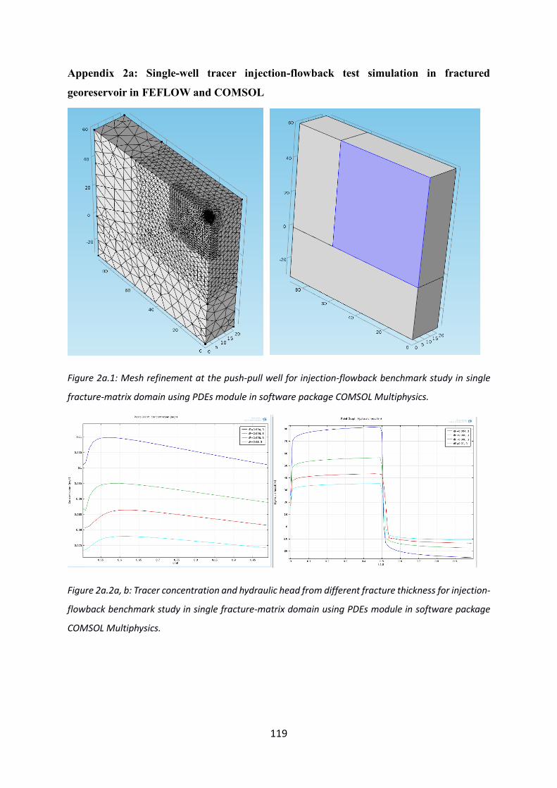
119

Appendix 2a: Single-well tracer injection-flowback test simulation in fractured

georeservoir in FEFLOW and COMSOL

Figure 2a.1: Mesh refinement at the push-pull well for injection-flowback benchmark study in single

fracture-matrix domain using PDEs module in software package COMSOL Multiphysics.

Figure 2a.2a, b: Tracer concentration and hydraulic head from different fracture thickness for injection-

flowback benchmark study in single fracture-matrix domain using PDEs module in software package

COMSOL Multiphysics.

120

Figure 2a.3a, b: Tracer concentration from different fracture thickness (8mm-left, 20mm-right) for

injection-flowback benchmark study in single fracture-matrix domain using PDEs module in software

package COMSOL Multiphysics.

121

Appendix 2b: A set of benchmark studies for flow and solute transport in geo-reservoir

Problem 2: 2D Dispersivity sensitivity study in different software with a mesh 40×80

Figure 2.1: MF/MT3DMS simulation concentration results for various longitudinal dispersivity, where

transversal dispersivity is 1/10 of longitudinal dispersivity for a constant input concentration 1mg/l in

the fluid flow of 17.28 m3/day

Figure 2.1: Problem 2:2D, FEFLOW simulation concentration results using using Full Upwinding method

for different longitudinal dispersivity, where transversal dispersivity is 1/10 of longitudinal dispersivity

0

0.2

0.4

0.6

0.8

1

0 20 40 60 80 100

Co

nce

ntr

atio

n m

g/l

Time (Days)

dL0

dL0.1

dL0.3

dL0.5

dL0.7

dL1

dL3

dL5

dL7

dL10

0

0.2

0.4

0.6

0.8

1

0 20 40 60 80 100

Co

nce

ntr

atio

n m

g/l

Time (Days)

dL0

dL0.1

dL0.3

dL0.5

dL0.7

dL1

dL3

dL5

dL7

dL10

122

for a constant input concentration 1mg/l in the fluid flow of 17.28 m3/day. FEFLOWsimulation result

shows smooth tracer simulation curves wheres ! shows strong numerical dispersion!

Figure 2.2: FEFLOW simulation concentration results using FEM Galerkin method for different

longitudinal dispersivity, where transversal dispersivity is 1/10 of longitudinal dispersivity for a

constant input concentration 1mg/l in the fluid flow of 17.28 m3/day

Figure 2.3: COMSOL simulation concentration results for different longitudinal dispersivity, where

transversal dispersivity is 1/10 of longitudinal dispersivity for a constant input concentration 1mg/l in

the fluid flow of 17.28 m3/day

0

0.2

0.4

0.6

0.8

1

0 20 40 60 80 100

Co

nce

ntr

atio

n m

g/l

Time (Days)

dL0.3

dL0.5

dL0.7

dL1

dL3

dL5

dL7

dL10

0

0.2

0.4

0.6

0.8

1

0 20 40 60 80 100

Co

nce

ntr

atio

n (

mg/

l)

Time (Days)

dL0.1

dL0.3

dL0.5

dL0.7

dL1

dL3

dL5

dL7

dL10

123

Figure 2.4: DUMUX simulation concentration results for different longitudinal dispersivity, where

transversal dispersivity is 1/10 of longitudinal dispersivity for a constant input concentration 1mg/l in

the fluid flow of 17.28 m3/day

Figure 2.5: MF/MT3DMS simulation concentration results for different discretization, where

transversal dispersivity is 1/10 of longitudinal dispersivity for a constant input concentration 1mg/l in

the fluid flow of 17.28 m3/day

0

0.2

0.4

0.6

0.8

1

0 20 40 60 80 100

Co

nce

ntr

atio

n m

g/l

Time (Days)

dL0

DL0.1

DL0.3

DL0.5

Dl0.7

dL1

dL3

dL5

dL10

0

0.1

0.2

0.3

0.4

0.5

0.6

0.7

0.8

0.9

1

0 10 20 30 40 50 60 70 80 90 100 110 120 130 140 150 160 170 180 190 200

Co

nce

ntr

atio

n m

g/L

Time (days)

1X

2X

4X

8X

16X

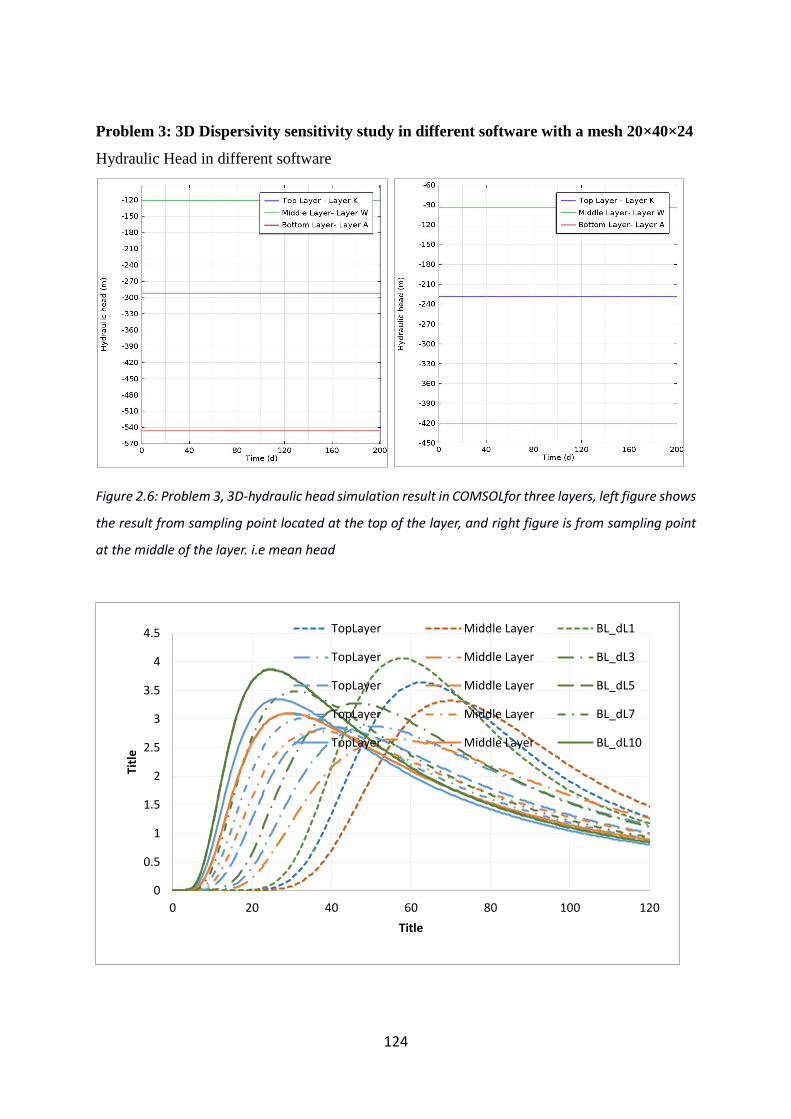
124

Problem 3: 3D Dispersivity sensitivity study in different software with a mesh 20×40×24

Hydraulic Head in different software

Figure 2.6: Problem 3, 3D-hydraulic head simulation result in COMSOLfor three layers, left figure shows

the result from sampling point located at the top of the layer, and right figure is from sampling point

at the middle of the layer. i.e mean head

0

0.5

1

1.5

2

2.5

3

3.5

4

4.5

0 20 40 60 80 100 120

Titl

e

Title

TopLayer Middle Layer BL_dL1

TopLayer Middle Layer BL_dL3

TopLayer Middle Layer BL_dL5

TopLayer Middle Layer BL_dL7

TopLayer Middle Layer BL_dL10

125

Figure 2.7: Dispersion sensitivity of tracer concentration simulated using MF/MT3DMS sampling at top

of the layer (a higher pressure than the mean pressure across the layer)

Figure 2.8: Dispersion sensitivity of tracer concentration simulated using MF/MT3DMS, sampling at

middle of the layer (assuming a mean pressure across the layer)

Comsol UG results on 3D simulation for Helez

Top Layer Middle layer Bottom layer

0

0.5

1

1.5

2

2.5

3

3.5

4

4.5

0 20 40 60 80 100 120

Co

nce

ntr

atio

n m

g/l

Time (days)

TopLayer Middle Layer

BL_dL10 TopLayer

Middle Layer BL_dL7

TopLayer Middle Layer

BL_dL5 TopLayer

Middle Layer BL_dL3

TopLayer Middle Layer

BL_dL1

126

Figures 2.10: Each pair of curves represent tracer BT at the top and middle sampling point of the layer

for a dispersivity value 1 m 3 m, 5 m, 7 m, 10 m. A higher concentration curves show from top sampling

point for each pair of curves

Figure 2.11: Problem 3, 3D-Simulation result on concentration spreading, at simulation time 200 days

in COMSOLfor three the layers, the figure shows the result from dispersivity value 3m, 5m, 7m and 10m

dispersivity value from left respectively.

127

List of Publications

List of publications that are authored or co-authored by me-

1. Karmakar, S., Ghergut, J., Sauter, M., 2015. Early-flowback tracer signals for fracture

characterization in an EGS developed in deep crystalline and sedimentary formations:

a parametric study, Geothermics, in press (Special issue on EGS),

2. Karmakar, S., Ghergut, I., Sauter, M., 2015. EGS in sedimentary basins: sensitivity of

early flowback tracer signals to induced-fracture parameters. Energy Procedia 76, 223-

229.

3. Rahman M.A., Karmakar S., Salama H., Gactha-Bandjun N., Btatkeu K. B.D.,

Noubactep C. (2013): Optimising the design of Fe0-based filtration systems for water

treatment: The suitability of porous iron composites. Journal of Applied Solution

Chemistry and Modeling, 2, 165-177. DOI: http://dx.doi.org/10.6000/1929-

5030.2013.02.03.2

Conference proceedings, poster, and oral presentation

1. DGMK/ÖGEW Frühjahstagung in Celle on 22 and 23 April 2015)

2. Deutsche Geophysikalische Gesellschaft (DGG) 75. Jahrestagung on 24 March 2015

abstracts

3. Benchmark study on flow and solute transport in geological reservoirs, Shyamal

Karmakar, Alexandru Tatomir, Sandra Oehlmann, Markus Giese, Martin Sauter

“Computational Method in Water Resource on 10-13 June 2014 at the University of

Stuttgart, Germany.”

4. Karmakar, S., Ghergut, I., Sauter, M., 2016, Early Time Flowback Test Tracer Selection

for Stimulated Georeservoir Fracture Characterization. Stanford Geothermal

Workshop, February 22-24

5. Co-operation or partial involvement with HEG M Sc. thesis work, During the Doctoral

study period 10.2012-04.2016

i. Tolulope Abiodun Owonibi: Numerical benchmark study of single phase flow and

transport in porous media (FEFLOW, COMSOL, and MODFLOW)

ii. Mr. Rizwan Mohsin: FSR study for Soulz-sous-Foret georeservoir and comparing

translatability of parameter betweeen geo-reservoirs as well as carbonate aquifer.

128

iii. Mr.Benjamin Olukunle Ekeade-Flow­storage repartitions (FSR) for tracer test

evaluation and geothermal reservoir characterization– analyzing data and models

of the Olkaria site in the East­Kenyan Rift Valley

129

Curriculum Vitae

Shyamal Karmakar

PERSONAL DATA

Date of birth- 20.11.1980

Place of birth- Barkal, Rangamati

Nationality- Bangladeshi

EDUCATION

10/2012 – Current Georg-August-Universität Göttingen Geoscience Centre Department Applied

Geology, Ph.D. Student

10/2009 – 11/2011 Georg-August-Universität Göttingen Geoscience Centre Department Applied

Geology (degree: M Sc. in Hydrogeology and Environmental Geoscience)

02/2007 – 12/2008 Institute of Forestry and Environmental Sciences, University of Chittagong,

M.S. in Environmental Science

01/2001 – 08/2006 Institute of Forestry and Environmental Sciences, University of Chittagong, B

Sc. in Environmental Science

WORK EXPERIENCE

Since 05/2012 Lecturer, Institute of Forestry and Environmental Sciences, University of

Chittagong, Bangladesh (On study leave since 08/2012)

02/2007– 09/2009 Institute of Forestry and Environmental Sciences, University of Chittagong, as

research assistant

130

Acknowledgement

My sincere thanks to my supervisors Professor Dr. Martin Sauter and Dr. Iulia Ghergut.

Particularly like to mention Dr. Iulia Ghergut’s extensive support throughout this period and

help me to develop and process ideas, confront with my mistakes! My special thanks and

gratitude to Professor Dr. Günter Buntebarth for his consent to assess my thesis as co-referee

at the very last moment. My sincere thanks to all other members of the Examination Board,

Professor Dr.-Ing. Thomas Ptak-Fix, Dr. Reinhard Jung and Dr. Ulrich Maier.

It has been a great occasion to work with Dr. Alex Tatomir and Dr. Sandra Oehlmann to create

a fruitful project on benchmark study; thanks buddies. Thanks to all my colleagues in Applied

Geology department, Ibrahim Hamadan, Markus Giese, Dr. Jannes Kordila, Dr. Torsten Lange,

PD Dr. Chicgoua Noubactep, Dr. Sebastian Schmidt, Dr. Yulan Jin, Dr. William Allokhoury,

Elena Shigorina, Peter Biermann, Anja Preglar, Dr. Matthias Franz, Mashia Mohammadfoghi,

Viet Cao, Monthon and others. It has been a quality time with you in various occasions and

discussion eventually does not limited to hydrogeology. Special thanks for Mrs. Beka Peters-

Kewitz and Mr. Hartmut Düker.

I like to thank my home University, Chittagong University to grant me the study leave and

keeping a place and opportunity to serve the country. I like to thank my teacher and colleagues

Prof. Dr. Sirajul Haque, Prof. Dr. Tapan Kumar Nath, Prof. Dr. Mohammad Jashimuddin, Prof.

Dr. Shafiul Alam, Tarit Kumar Bal and current director of the IFESCU Prof. Dr. Khaled

Mizbahuzzaman and for their encouragement and support at many stages to avail this study

leave and keep me motivated to accomplish my higher study. Thanks to my friends of Batch

22 and seniors of the institute who are always by my side in any needs of help.

I like to thank the small Bengali community, which has kept my memory and affection alive to

the country.

Obviously my warmest thanks to my wife Mandira for her unconditional support and

acceptance of my impatience and clumsy time. To my son Apratim (who has many complain

about my disappearance during afternoon and evening time!), I hope you will forget this phase

and forgive me, thanks for the sacrifice and understanding! My parents, especially my Mother,

your inspiration, and sacrifice built me, kept me motivated at any stage of depression; as I

know, the challenge you have faced and overcame, my struggle counts nothing to it!

131

It is an excellent opportunity to achieve the finance and support from DAAD to continue this

Ph.D. study. I should not forget the insurance, and administrative support from DAAD, also

noteworthy to mention a nice opportunity to have a Deutschkurs in Leipzig. It is a great

occasion for me to learn the language and culture also to live in Leipzig for four months. I do

love to continue the journey in this language and culture! I promise.