Single Point Gradiometer for Planetary Applications José Luis Mesa , Marina Díaz Michelena , David Ciudad , Whitney Schoenthal Michael E. McHenry , Marco Maicas , and Claudio Aroca

Abstract—We have designed and fabricated a microelectromechanical device, based on the alternating field gradient concept, to measure surface magnetic field gradient on planets. Its sensitivity is 4 x10~4 T/m, which is appropriate for magnetite outcrops and areas with rocks formed at different stages recording geomagnetic field reversals. We present the results obtained with three different prototypes.

Index Terms—Magnetic instruments, gradient methods, microelectromechanical system, microsensors.

I. INTRODUCTION II. METHODOLOGY

Crustal sources are an important contribution to planetary magnetic fields (Earth) and the primary contribution when no global field remains (Mars/Moon) [Langlais 2004]. To unam­biguously distinguish these sources is a complex problem. Mea­surements at different altitudes or measuring derivatives of the field would improve the convergence of the solution.

This study complements current magnetic ground surveys with instruments capable of measuring the magnetic field gradi­ent. The field produced by Earth lithospheric anomalies ranges from -3700 to 8300 nT at a low Earth orbit of 450 km from the surface. On ground, high (spatial) resolution surveys in geologi­cal structures with an associated magnetic signature (magnetite outcrops, volcanoes, impact craters, basaltic intrusions, etc.) range from 0.1 to 100/xT [Michelena 2015]. Resolutions on the order of 10~8-10~6 T/m are necessary for accurate on-ground geophysical surveys: to identify magnetic minerals like mag­netite, pyrrhotite, and hematite, and different mineral phases (titanomagnetites) on Earth [Sanz2011]. Rougher sensitivities are still interesting for strong field contrasts like the magnetite outcrop of El Laco, Chile (>100.000 nT in <1 m) [Michelena 2015], some areas with high remanence rocks formed dur­ing different ages, including geomagnetic field reversals, and probably for the strong magnetic anomalies reported on Mars [Dunlop2005].

We describe a single point gradiometer named for the short spatial base of the measurements (mm) compared with the wavelength of most magnetic anomalies in geological structures (cm to km).

The magnetic induction vector B will be referred as the mag­netic field. The magnetic field gradient is composed of nine ele-ments represented by a symmetric tensor v 2 , where §* = % in the absence of electrical currents or time varying electric fields (V x B = 0). Here, we focus on a nondiagonal component of the tensor. However, the system can be easily adapted to measure the other five components of the gradient.

The determination of magnetic field gradient is based on ideas used in alternating gradient/force magnetometers (AGM/AFM). In an AFM, a sample is vibrated by means of a magnetic force and the vibration amplitude is measured by opti­cal, capacitive, or other contactless detectors. Many micromag-netic devices [Moreland 2003] have been constructed based on principles of AGM, torsional oscillator [Yin 2013], or the sym­metric vibrating-sample magnetometer (VSM) [Ziljstra 1967]. In the past, we have used AFMs [Michelena 2000] to measure magnetic properties of sputtered thin films of low magnetic mo­ment due to the comparative advantages of AFM as compared with VSM: lower noise and better resolution.

Similar devices have been previously reported including a gradiometer developed by Sunderland [2008] based on an alu­minum wire (0.25 m length) with better resolution which has been qualified for space applications.

Three AFM-based microelectromechanical (MEMS) proto­types of low noise and high resolution have been developed to measure the gradient of the magnetic field [Ciudad 2009]. The physical principle and characteristics of the device are de­scribed in the following. The potential energy U of a magnetic dipole moment m in the presence of a magnetic field is

U = -m-B. (1)

The magnetic force F is derived as the gradient of the poten­tial energy:

F = -VU = V(m • B). (2)

Assuming that a magnetic dipole

ih = mxi (3)

is attached to a mechanical cantilever, in the presence of a magnetic field with a single component in the x direction

B = BJ (4)

which varies spatially along the z direction

n = ^k (5)

Ferromagnetic ribbon

(a)

¿^Bimcfrrph(

Lock-in amplifier

^ 5 ^ J

fPhotodiode

Infrared LED Permanent magnets i z

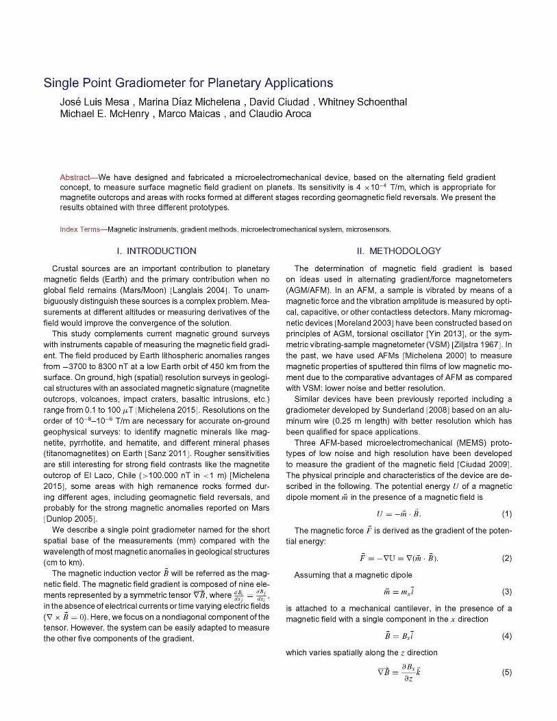
(OBJdz) h Fig. 1. Diagram for setups: (a) piezoelectric detection method (prototype 1); (b) optoelectronic detection (prototypes 2 and 3).

Table 1. Ferromagnetic ribbons properties.

Thickness

Length

Width

Saturation Induction

Magnetostriction

FMA \ 2826MB

29 ¡xm

20 mm

1.5 mm

0.88 T

12 ppm

FMB \ 2705M

22 ¡xm

20 mm

1.5 mm

0.77 T

< 0.5 ppm

the force contribution is (only z direction)

dBx

F, = mx . dz

(6)

In this setup (see Fig. 1), commercial soft magnetic materials

by Metglas (see Table 1) are attached at the end of a cantilever.

The magnetic material is magnetized in an alternating field Bx(t),

acquiring an alternating dipole mx(t).

In a magnetic field gradient [see (5)], the free end of a can­

tilever experiences an alternating force along z-axis [see (6)]

and vibrates. If the frequency of the force is tuned at the can­

tilever's mechanical resonance frequency, in the absence of an

external gradient, the amplitude of the vibration is maximized

and the phase exhibits a maximum shift {6 = 180°). In an exter­

nal field gradient parallel to the exciting gradient [see (5)], the

cantilever oscillation will change in amplitude and phase.

Thus, knowing the exciting gradient and magnetic moment

amplitude of the sample, it is possible to determine external

gradients, by monitoring the vibrational properties.

In our prototypes, the vibration is characterized by piezo­

electric effect and optically. The cantilever is a bimorph, which

consists of two stacked piezoelectric plates of lead zirconate

titanate (PZT): of dimensions 60 x 20 x 0.7 mm3—cantilever

A; and 40 x 20 x 0.7 mm3—cantilever B, inversely polarized to

bend the system. An estimation of the force resolution limit for

a vibrating cantilever due to thermal noise is given by Stowe

[1997]. Extrapolating the results of the magneticforce produced

by the magnetization of the ribbons on the cantilever («10~6 N)

and comparing it with the limit force resolution («10~1 0 N), we

assume that we are far enough from this limit to ignore thermal

noise effects in our results. The changes in vibration are read

by the induced piezoelectric voltage.

The optical detection is based on the different light cone, i.e.,

light intensity received by a photodiode, after being reflected

by a surface, depending on the relative distance between the

reflecting surface and the optical collector [Lucas 2009]. This

method is preferred to beam bounce [Yin 2013] and others

for its compactness. The light source is a light emitting diode

(LED) and the detector is a photodiode [see Fig. 1(b)]. The

light is transmitted to the vibrating structure by an optical fiber

and collected by six optical outer fibers (daisy configuration

array) to guide it back to the photodetector. The array is placed

perpendicular to the sample and the LED light reflects off the

sample and is collected by the outerfibers. This system provides

higher resolution (4 nm) than piezoelectric detection (1 /xm).

III. E X P E R I M E N T A L R E S U L T S

Based on the methodology described in Section II, three dif­

ferent macroscopic setups have been evaluated in terms of their

magnetic properties: resolution, long term stability, and sensi­

tivity, and other aspects as power consumption and complexity.

The three devices have been characterized in the presence of

an external field gradient produced by a magnetized sample ap­

proached at a controlled distances from the vibrating cantilever,

previously quantified in the position of the cantilever by means

of a magnetometer. The corresponding external field gradient

is obtained by measuring the field at different distances. Along

the approach direction, changes in amplitude and phase are

monitored. The changes in the oscillation amplitude and phase

are represented as a function of the field gradient created by

the sample, demonstrating linear dependence and sign sensi­

tivity. Next, we describe the three prototypes developed and

their main characteristics.

A. Prototype 1

In this prototype, the mechanical structure is the Cantilever

A made of a bimorph material. On its surface it has a set of

six Metglas 2826 MB magnetic ribbons FMA (see Table 1),

attached close to the free end of the cantilever such that the long

dimension of the ribbons is set perpendicular to the length of the

cantilever. The ribbons are magnetized along their length with

an alternating magneticf ieldsothat ineach cycle, an alternating

dipole is set in both directions of the x-axis in the free end of

the cantilever. Metglas ribbons were selected as a commercial

soft magnetic material of high permeability and low coercivity,

which facilitates ac magnetization.

Due to the low resonance frequency of the system (42 Hz),

an electromagnet was used to magnetize the ribbons (10 mT

max.). A set of four permanent magnets were used to pro­

vide the magnetic field gradient [setup is depicted in Fig. 1(a)].

In this first prototype, the vibration is monitored by means of

piezoelectric effect. If the bimorph is made of two piezoelec­

tric layers, when the cantilever vibrates, the layers stretch and

contract, setting an electrical voltage across them. The oscil­

lating voltage is measured with a lock-in amplifier. This system

was subjected to well-known external gradients in a range of

0.25 T/m. Fig. 2 shows the results in amplitude and phase.

This first prototype shows limitations in both excitation and

detection. On the one hand, the dimensions of the soft mag­

netic ribbons make their magnetization to saturation difficult

3,0

2'51

>2'°1 E >1,5-

< 1,0-

0,5-

\ Xx-

--''

•

.y''" V

,•"" , .A

/ V ^\

Bx-X.

--4 S

-6 -7

--8 q

- 1 0 --11

--12

(a) Surface Mag negation

-0,30 -0,25 -0,20 -0,15 -0,10 -0,05 8Bx/8z (T/m)

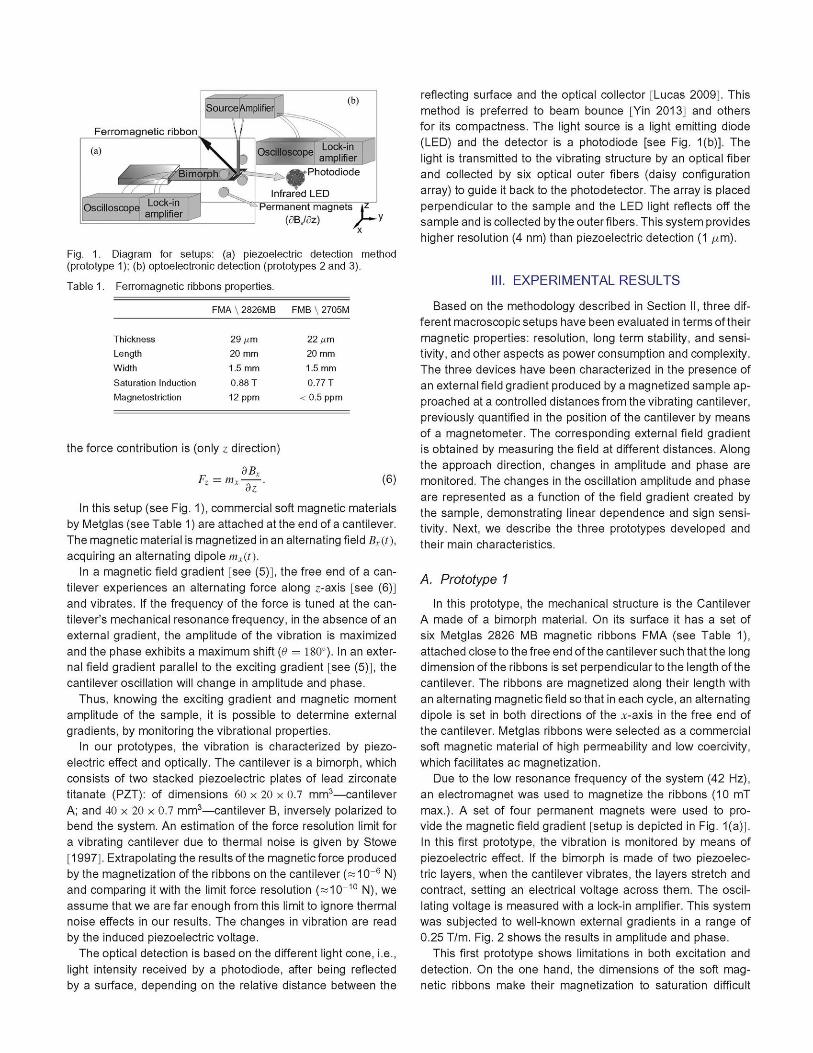
Fig. 2. Prototype 1 results: amplitude (black) and phase (grey).

due to the relatively high demagnetizing factor, and the power budget is excessive (electromagnet consumption up to 20 W). Also, 2826 MB/FMA (see Table 1) ribbon is highly magne-tostrictive (12 ppm) compared to other ribbons like 2705 M/FMB (< 0.5 ppm) and this may imply noncontrolled effects. On the other hand, the piezoelectric detection has a restricted sensitiv­ity with resolutions on the order of 1-10 /¿m.

The external gradient used in this prototype is negative, and adds to the permanent gradient (generated by the magnets), which is also negative, producing an increase of the signal am­plitude with an increase of the external gradient amplitude (see Fig. 2). In case the permanent gradient is positive (prototypes 2 and 3), a negative value of the external gradient would gener­ate a decrease in the oscillating amplitude, as it will be shown in the calibration curve for prototype 3 [see calibration inset in Fig. 4(a)]. This demonstrates the ability of the system to be sign sensitive to the voltage changes.

B. Prototype 2

This device improves some of the limitations of the former prototype. In this case, the ribbon used is FMB, Metglas 2705 M (low magnetostriction), magnetized by means of an electrical current instead of coils to improve the power efficiency, and on the other hand, the detection is carried out optically to improve the resolution. The complexity of this setup is slightly higher than that of prototype 1.

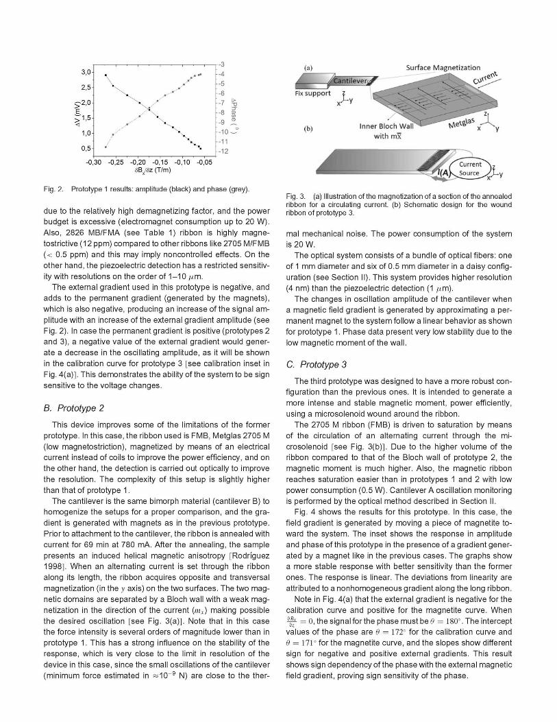
The cantilever is the same bimorph material (cantilever B) to homogenize the setups for a proper comparison, and the gra­dient is generated with magnets as in the previous prototype. Prior to attachment to the cantilever, the ribbon is annealed with current for 69 min at 780 mA. After the annealing, the sample presents an induced helical magnetic anisotropy [Rodriguez 1998]. When an alternating current is set through the ribbon along its length, the ribbon acquires opposite and transversal magnetization (in the y axis) on the two surfaces. The two mag­netic domains are separated by a Bloch wall with a weak mag­netization in the direction of the current K ) making possible the desired oscillation [see Fig. 3(a)]. Note that in this case the force intensity is several orders of magnitude lower than in prototype 1. This has a strong influence on the stability of the response, which is very close to the limit in resolution of the device in this case, since the small oscillations of the cantilever (minimum force estimated in «10~9 N) are close to the ther-

Fix support

^tarrt i leyer^'

JU

Ih) Inner Bloch Wall with mx

Fig. 3. (a) Illustration of the magnetization of a section of the annealed ribbon for a circulating current, (b) Schematic design for the wound ribbon of prototype 3.

mal mechanical noise. The power consumption of the system is 20 W.

The optical system consists of a bundle of optical fibers: one of 1 mm diameter and six of 0.5 mm diameter in a daisy config­uration (see Section II). This system provides higher resolution (4 nm) than the piezoelectric detection (1 /¿m).

The changes in oscillation amplitude of the cantilever when a magnetic field gradient is generated by approximating a per­manent magnet to the system follow a linear behavior as shown for prototype 1. Phase data present very low stability due to the low magnetic moment of the wall.

C. Prototype 3

The third prototype was designed to have a more robust con­figuration than the previous ones. It is intended to generate a more intense and stable magnetic moment, power efficiently, using a microsolenoid wound around the ribbon.

The 2705 M ribbon (FMB) is driven to saturation by means of the circulation of an alternating current through the mi­crosolenoid [see Fig. 3(b)]. Due to the higher volume of the ribbon compared to that of the Bloch wall of prototype 2, the magnetic moment is much higher. Also, the magnetic ribbon reaches saturation easier than in prototypes 1 and 2 with low power consumption (0.5 W). Cantilever A oscillation monitoring is performed by the optical method described in Section II.

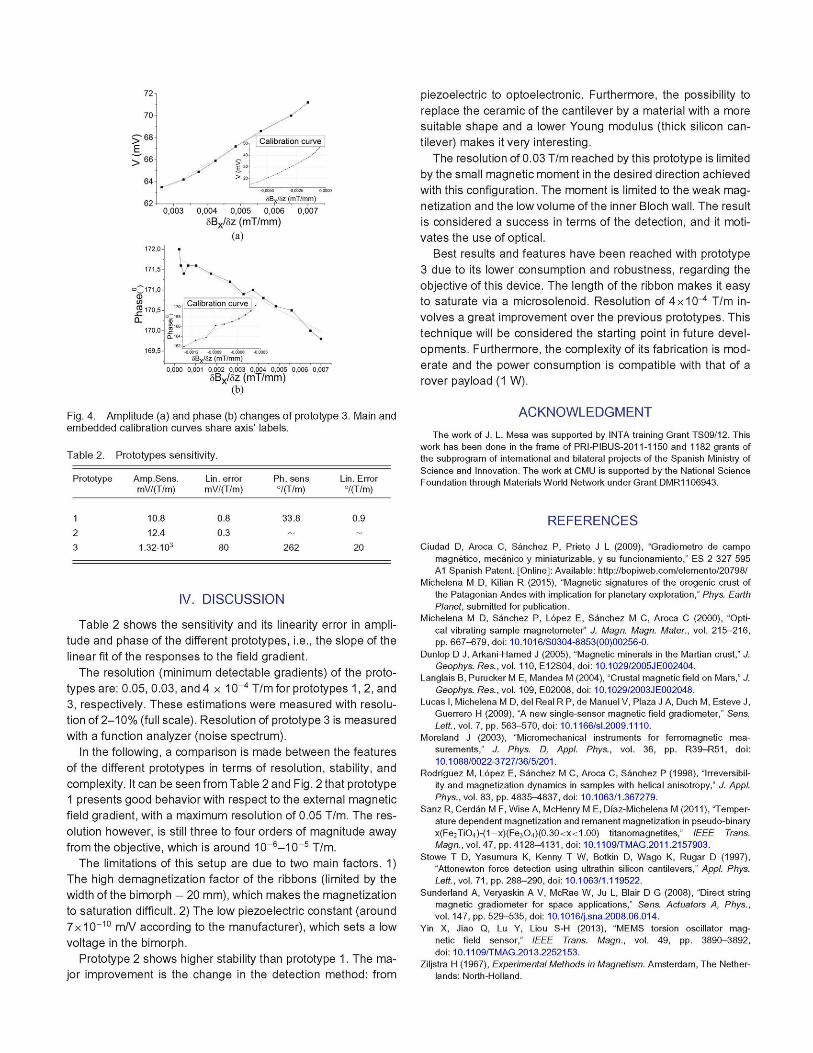
Fig. 4 shows the results for this prototype. In this case, the field gradient is generated by moving a piece of magnetite to­ward the system. The inset shows the response in amplitude and phase of this prototype in the presence of a gradient gener­ated by a magnet like in the previous cases. The graphs show a more stable response with better sensitivity than the former ones. The response is linear. The deviations from linearity are attributed to a nonhomogeneous gradient along the long ribbon.

Note in Fig. 4(a) that the external gradient is negative for the calibration curve and positive for the magnetite curve. When ^|- = 0, the signal for the phase must be 6 = 180°. The intercept values of the phase are 6 = 172° for the calibration curve and e = 171° for the magnetite curve, and the slopes show different sign for negative and positive external gradients. This result shows sign dependency of the phase with the external magnetic field gradient, proving sign sensitivity of the phase.

70

> E 66

**

¿ r \ -

Calibration curve |

^ / * < - * • •

6BX/Sz (mT/mm)

0,003 0,004 0,005 0,006 0,007

5Bx/8z (mT/mm) (a)

172,0

171,5

<=C171,0

J1 7 0 5 170,0

169.5H •0,0012 -0,0009

Bx/Sz (mT/mm)

0,000 0,001 0,002 0,003 0,004 0,005 0,006 0,007

5Bx/5z (mT/mm) (b)

Fig. 4. Amplitude (a) and phase (b) changes of prototype 3. Main and embedded calibration curves share axis' labels.

Table 2. Prototypes sensitivity.

Prototype

1

2

3

Amp.Sens. mV/(T/m)

10.8

12.4

1.32-103

Lin. error mV/(T/m)

0.8

0.3

80

Ph.sens D/(T/m)

33.8

-262

Lin. Error D/(T/m)

0.9

-20

IV. DISCUSSION

Table 2 shows the sensitivity and its linearity error in ampli­tude and phase of the different prototypes, i.e., the slope of the linear fit of the responses to the field gradient.

The resolution (minimum detectable gradients) of the proto­types are: 0.05, 0.03, and 4 x 10~4 T/m for prototypes 1,2, and 3, respectively. These estimations were measured with resolu­tion of 2-10% (full scale). Resolution of prototype 3 is measured with a function analyzer (noise spectrum).

In the following, a comparison is made between the features of the different prototypes in terms of resolution, stability, and complexity. It can be seen from Table 2 and Fig. 2 that prototype 1 presents good behavior with respect to the external magnetic field gradient, with a maximum resolution of 0.05 T/m. The res­olution however, is still three to four orders of magnitude away from the objective, which is around 10~6-10~5 T/m.

The limitations of this setup are due to two main factors. 1) The high demagnetization factor of the ribbons (limited by the width of the bimorph - 20 mm), which makes the magnetization to saturation difficult. 2) The low piezoelectric constant (around 7x10~10 m/V according to the manufacturer), which sets a low voltage in the bimorph.

Prototype 2 shows higher stability than prototype 1. The ma­jor improvement is the change in the detection method: from

piezoelectric to optoelectronic. Furthermore, the possibility to replace the ceramic of the cantilever by a material with a more suitable shape and a lower Young modulus (thick silicon can­tilever) makes it very interesting.

The resolution of 0.03 T/m reached by this prototype is limited by the small magnetic moment in the desired direction achieved with this configuration. The moment is limited to the weak mag­netization and the low volume of the inner Bloch wall. The result is considered a success in terms of the detection, and it moti­vates the use of optical.

Best results and features have been reached with prototype 3 due to its lower consumption and robustness, regarding the objective of this device. The length of the ribbon makes it easy to saturate via a microsolenoid. Resolution of 4x1o -4 T/m in­volves a great improvement over the previous prototypes. This technique will be considered the starting point in future devel­opments. Furthermore, the complexity of its fabrication is mod­erate and the power consumption is compatible with that of a rover payload (1 W).

ACKNOWLEDGMENT

The work of J. L. Mesa was supported by INTA training Grant TS09/12. This

work has been done in the frame of PRI-PIBUS-2011-1150 and 1182 grants of

the subprogram of international and bilateral projects of the Spanish Ministry of

Science and Innovation. The work at CMU is supported by the National Science

Foundation through Materials World Network under Grant DMR1106943.

REFERENCES

Ciudad D, Aroca C, Sánchez P, Prieto J L (2009), "Gradiometro de campo

magnético, mecánico y miniaturizable, y su funcionamiento," ES 2 327 595

A1 Spanish Patent. [Online]: Available: http://bopiweb.com/elemento/20798/

Michelena M D, Kilian R (2015), "Magnetic signatures of the orogenic crust of

the Patagonian Andes with implication for planetary exploration," Phys. Earth

Planet, submitted for publication.

Michelena M D, Sánchez P, López E, Sánchez M C, Aroca C (2000), "Opti­

cal vibrating sample magnetometer" J. Magn. Magn. Mater., vol . 215-216,

pp. 667-679, doi: 10.1016/S0304-8853(00)00256-0.

Dunlop D J, Arkani-Hamed J (2005), "Magnetic minerals in the Martian crust," J.

Geophys. Res., vol. 110, E12S04, doi: 10.1029/2005JE002404.

Langlais B, Purucker M E, Mandea M (2004), "Crustal magnetic field on Mars," J.

Geophys. Res, vol. 109, E02008, doi: 10.1029/2003JE002048.

Lucas I, Michelena M D, del Real R P , de Manuel V, Plaza J A, Duch M, Esteve J,

Guerrero H (2009), "A new single-sensor magnetic field gradiometer," Sens.

Lett., vol. 7, pp. 563-570, doi: 10.1166/sl.2009.1110.

Moreland J (2003), "Micromechanical instruments for ferromagnetic mea­

surements," J. Phys. D, Appl. Phys, vol. 36, pp. R 3 9 - R 5 1 , doi:

10.1088/0022-3727/36/5/201.

Rodríguez M, López E, Sánchez M C, Aroca C, Sánchez P (1998), "Irreversibil­

ity and magnetization dynamics in samples with helical anisotropy," J. Appl.

Phys., vol. 83, pp. 4 8 3 5 ^ 8 3 7 , doi: 10.1063/1.367279.

Sanz R, Cerdán M F, Wise A, McHenry M E, Díaz-Michelena M (2011), 'Temper­

ature dependent magnetization and remanent magnetization in pseudo-binary

x(Fe2TiO4)-(1-x)(Fe3O4)(0.30<x<1.00) titanomagnetites," IEEE Trans.

Magn., vol. 47, pp. 4128 -4131 , doi: 10.1109/TMAG.2011.2157903.

Stowe T D, Yasumura K, Kenny T W, Botkin D, Wago K, Rugar D (1997),

"Attonewton force detection using ultrathin silicon cantilevers," Appl. Phys.

Lett., vol. 7 1 , pp. 288-290, doi: 10.1063/1.119522.

Sunderland A, Veryaskin A V, McRae W, Ju L, Blair D G (2008), "Direct string

magnetic gradiometer for space applications," Sens. Actuators A, Phys.,

vol. 147, pp. 529-535, doi: 10.1016/j.sna.2008.06.014.

Yin X, Jiao Q, Lu Y, Liou S-H (2013), "MEMS torsion oscillator mag­

netic field sensor," IEEE Trans. Magn., vol. 49, pp. 3890-3892,

doi: 10.1109/TMAG.2013.2252153.

Ziljstra H (1967), Experimental Methods in Magnetism. Amsterdam, The Nether­

lands: North-Holland.