Single-Photon Detection Using Optical Heterodyne Interferometry

Zachary Bush1, Simon Barke1, Harold Hollis1, Aaron D. Spector2, Ayman Hallal1, D.B. Tanner 1, Guido Mueller11Department of Physics, University of Florida, PO Box 118440, Gainesville, Florida, 32611, USA

2Deutsches Elektronen-Synchrotron (DESY), Notkestrae 85, D-22607 Hamburg, Germany(Dated: March 29, 2018)

We explore the application of heterodyne interferometry for a weak-field coherent detectionscheme. The methods detailed here will be used in ALPS II, an experiment designed to searchfor weakly interacting sub-eV particles. For ALPS II to reach its design sensitivity this detectionsystem must be capable of accurately measuring fields with an amplitude equivalent to 10−6 photonsper second. We present initial results of an equivalent dark count rate of better than 10−6 photonper second as well as successful generation and detection of a signal with a field strength equivalentto 10−2 photons per second.

OCIS codes: (040.2840) Heterodyne; (140.0140) Lasers and laser optics

I. INTRODUCTION

I.1. Axions and Axion-Like Particles

The Standard Model (SM) incorporates our currentknowledge of subatomic particles as well as their interac-tions via three of the four fundamental forces of nature.The SM is not complete, however, as it does not containgravity and does not explain certain observations. One no-table unresolved issue is that of charge-conjugation paritysymmetry (CP-symmetry) violation. The QCD Lagrangianincludes terms capable of breaking CP symmetry for thestrong force. In contrast, experimentation finds that thestrong forces respect CP-symmetry to a very high preci-sion [1].

The most prominent proposed solution, introduced byPeccei and Quinn [2], involves spontaneously breaking aglobal U(1) symmetry leading to a new particle, namedthe axion [3, 4]. Interactions with the QCD vacuum causethe axion to have a non-zero mass, ma [2]. While axionsmay interact with SM particles, most notably for exper-imental purposes, axion mixing with neutral pions leadsto a characteristic two photon coupling, gaγγ [5]. This, inturn, constrains the product of the axion mass and couplingsuch that these two parameters are dependent. Experimen-tal and observational factors place the axion mass between1 and 1000 µeV. The corresponding range for gaγγ is 10−16

to 10−13 GeV−1.

While the QCD axion is confined to a specific band ofparameter space, it might just be a member of a larger classof axion-like particles with a stronger two photon coupling[6, 7]. The interactions between these axions/axion-likeparticles and photons may possibly explain unanswered as-tronomical questions including TeV photon transparencyin the Universe [8] and anomalous white dwarf cooling [9].The intrinsic properties of axions and axion-like particlesalso make them prime candidates for cold dark matter.This theoretical motivation has led to the formulation ofvarious experiments designed to detect axions and axion-like particles by utilizing their coupling to photons.

Although axions can naturally decay into two observablephotons, the rate at which this occurs is extremely low,making detection impossible. Axion search experimentstherefore also rely on the inverse Primakoff or Sikivie effect

in which a strong static magnetic field acts as a high densityof virtual photons. This stimulates the axion/axion-likeparticle to convert into a photon carrying the total energyof the axion/axion-like particle [10, 11]. These experimentsemploy different strategies to look for axions from varioussources. Haloscope experiments, such as ADMX, use reso-nant microwave cavities and strong superconducting mag-nets to search for axions comprising the Milky Way’s darkmatter halo [12]. Helioscope experiments, such as CAST,look for relativistic axions originating from the Sun thatconvert into detectable X-rays as they pass through a sup-plied magnetic field [13]. Differing from these types of axionsearches that rely on astronomical sources, “Light Shiningthrough Walls” (LSW) experiments attempt to generateand detect axions in the laboratory and are therefore notdependent on models of the galactic halo or on models ofstellar evolution [14–16].

I.2. ALPS II

LSW experiments use the axion-photon coupling first toconvert photons into axions under the presence of a strongmagnetic field. These axions then pass through a light-tightbarrier. They travel through another strong magnetic fieldand some are reconverted back into detectable photons.Energy is conserved in the process, so that the regeneratedphotons behind the wall have the same energy as those in-cident in front of it. The Any Light Particle Search (ALPS)is one such LSW experiment. The first generation of thisexperiment, ALPS I, set the most sensitive experimentallimits of its time on the coupling of axions to two photons,gaγγ , for a wide range of axion masses [17]. ALPS I useda single optical cavity placed before a light tight barrierto increase the circulating power on the axion generationside of the magnet. The second iteration of the experi-ment, ALPS II, will improve the sensitivity further withthe addition of an optical cavity after the barrier. Thepresence of this cavity will resonantly enhance the proba-bility that axions/axion-like particles will reconvert to pho-tons [18, 19]. ALPS II is currently being developed in twostages. The first stage, ALPS IIa, will use two 10 meterresonant cavities without magnets [20]. The second stage,ALPS IIc, will use 100 m long cavities with 5.3 T super-conducting HERA dipole magnets. Longer cavity lengths

arX

iv:1

710.

0420

9v3

[ph

ysic

s.in

s-de

t] 2

8 M

ar 2

018

2

increase the interaction time between the photons and themagnetic field.

FIG. 1. Simplified model of the ALPS IIc experiment. Axionsgenerated in the left-hand side cavity traverse the wall and turnback into detectable photons in the right-hand side cavity

.

Figure 1 shows a simplified layout of the ALPS IIc exper-iment. Infrared laser light is injected into an optical cavitywhose eigenmode is immersed in a 5.3 T magnetic field.The polarization is set so that the electric field of the laserlight is parallel to the transverse magnetic field of the dipolemagnet. Power buildup from this cavity causes a high cir-culating laser power, increasing the flux of axion-like par-ticles through the wall. After these particles traverse thelight-tight barrier they enter a second cavity, called the re-generation cavity, also subject to a 5.3 T magnetic field.The particles then have the same probability to reconvertback into photons with the original energy as the initialfield

Improvements from ALPS I to ALPS IIc lead to a a 2000-fold increase in sensitivity on the coupling parameter, gaγγ ,shown in Fig. 2.

Mass ma in eV

Cou

plin

g co

nsta

nt g

aγγ

in G

eV−1

10–5 10–4

10–11

10–10

10–9

10–8

10–7

10–6

10–5

ALPS–IIc

ALPS–I

10–3

FIG. 2. Parameter space of the axion mass (ma) and cou-pling (gaγγ) showing projected improvements in sensitivity fromALPS I to ALPS IIc [19]. For ALPS IIc, such sensitivity in theaxion-photon coupling would require 4 weeks of measurementtime for a 5-sigma confidence in the limit, or in a detection atthe lower limit of sensitivity.

Based on the current experimental parameters for ALPSIIc, the expected sensitivity limit of the regenerated photonpower is on the order of 10−24 W. For 1064 nm light, this isequivalent to a rate of 2×10−5 photons per second. There-fore, integration times significantly longer than 12 hoursare required for confident detection. ALPS II is exploring

two technologies for detecting such weak signals. The firstof these uses a transition edge sensor [21]. This technol-ogy utilizes superconducting materials operating near theirphase transition temperature. An alternative approach,heterodyne interferometry, is the subject of this paper [18].

I.3. Heterodyne Detection Principles

The principle of heterodyne interferometry requires in-terfering two laser fields at a non-zero difference frequency.Let one laser, L1, have frequency f , phase φ1, and averagepower P1 and a second laser, L2, have frequency f + f0,phase φ2, and average power P2. Optically mixing theselasers at a photodetector yields the following expression:

∣∣∣√P1ei(2πft+φ1) +

√P2e

i[2π(f+f0)t+φ2]∣∣∣2 =

P1 + P2 + 2√P1P2 cos (2πf0t+ ∆φ) . (1)

Here, we have written the laser fields as proportional tothe square root of the average power and have set ∆φ =φ2 − φ1. While the first two terms on the right side of theequation are the individual DC powers, the third term isa time varying signal, called a beat note, at the differencefrequency, f0.

In our implementation of the heterodyne readout, thedetector photocurrent, represented by Eq. 1, is digitizedsatisfying the Nyquist criterion for sampling signals at f0.The band-limited signal is then mixed to an intermediatefrequency and written to file using a Field ProgrammableGate Array (FPGA) card. Then, a second mixing stagein post-processing shifts the signal to DC, splitting it intotwo quadratures. Each resultant quadrature is continu-ously integrated over the measurement time. In order forthe signal to accumulate, phase coherence between the twolaser fields must be maintained during this entire process.The two quadratures are then combined in such a way tocompute a single quantity proportional to the product ofthe photon rate of each laser.

Implementation of a heterodyne detection scheme inALPS II will involve injecting a second laser, phase co-herent with the signal field, into the regeneration cavityat a known offset frequency. The overlapped beams aretransmitted out of the cavity and are incident onto theheterodyne detector.

In this report we present results from a test setup whichvalidates the approach and will guide its implementationinto ALPS IIc. To begin, in Section II we mathematicallydemonstrate how a coherent signal is extracted from theinput. In Section III, we then discuss the optical designcreated to test this technique and the digital design whichforms the core of heterodyne detection. Finally, in Sec-tion IV we present results on device sensitivity and coher-ent signal measurements.

3

II. MATHEMATICAL EXPECTATIONS

II.1. Signal Behavior

In our standalone experiment, two lasers are interferedand incident onto a photodetector. Laser 1 acts as ourlocal oscillator (LO) with average power PLO while Laser2 is the weak signal field we wish to measure with aver-age power Pweak. The difference frequency is set such thatthe generated beat note has frequency fsig. Once the com-bined beam is incident onto a photodetector with gain G inV/W, it is digitized into discrete samples, n, at samplingfrequency fs. Sampling is done using an analog-to-digitalconverter (ADC) with a 1 V reference voltage. In the ab-sence of noise, the AC component of the signal becomes

xsig[n] = 2G√PLOPweak cos (2π

fsigfs

n+ φ) , (2)

where φ is an unknown but constant phase.In order to recover amplitude information, the digitized

signal is separately mixed with a cosine/sine wave at fre-quency fd = fsig in a process known as I/Q demodulation:

I[n] = xsig[n]× cos (2πfdfsn)

Q[n] = xsig[n]× sin (2πfdfsn) .

(3)

Each quadrature is individually summed from n = 1 toN samples. The squared sums are added together andnormalization is done through division by N2. This entirequantity is given by the following expression,

Z(N) =(∑Nn=1 I[n])2 + (

∑Nn=1Q[n])2

N2. (4)

The numerator is in fact the square of the magnitude of thediscrete Fourier transform (DFT) of the digitized input1

evaluated at fdfs

:

Z(N) =|X[ fdfs ]|2

N2, (5)

where

X[fdfs

] =

N∑n=1

x[n]e−i2πfdfs

(n−1) . (6)

Setting fd = fsig and solving for Z(N) with an input givenby Eq. 2 yields,

Zsig(N) = G2PLOPweak . (7)

Demodulating at the signal frequency causes Z(N) to beproportional to Pweak and constant with integration time,τ . The power in the local oscillator amplifies the beat noteamplitude and will be set to overcome all technical noisesources.

1 It must be noted that this is only exactly true in the case thatfdfs

= kN

for some integer k. If this requirement is not met then the

windowing process results in spectral leakage and Z(N) becomesan estimate of the DFT. However, in the large N limit this leakagebecomes negligible.

II.2. Noise Behavior

We wish to set the weak signal field to compare with theexpected sensitivity of ALPS IIc on the order of a few pho-tons per week. Therefore we must consider the influenceof important noise sources such as laser relative intensitynoise and optical shot noise. In order to understand the in-fluence of such noise, let us determine Z(N) in the absenceof an RF signal (Pweak = 0) but in the presence of noise.

Consider the input x[n] to be a random station-ary process. The quantity Znoise(N) can be writtenin terms of the single-sided analog power spectral den-sity (PSD) evaluated at the demodulation frequency,fd. To do so, we first convert the analog PSD inV2/(cycles per second) to the digitized power spectral den-sity (DPSD) in V2/(cycles per sample) using the samplingfrequency fs [22].

DPSD

(fdfs

)= fs PSD(fd) (8)

The DPSD is related to the expectation, E , of the DFT ofx[n] [22]:

DPSD

(fdfs

)= limN→∞

E

[|X[ fdfs ]|2

N

]. (9)

Using Eq. 5 we can solve for Z(N).

limN→∞

E [Znoise(N)] =PSD(fd)

τ, (10)

where we use the substitution N = τfs. It is important tonote that this only depends upon the PSD evaluated at fdand not across the entire spectrum.

Although Eq. 10 exactly relates the expectation value ofZnoise(N) to the analog PSD, we are interested in the resultof a single trial. For such an individual trial, Znoise(N)provides only an estimate of the analog PSD. Because thenoise is assumed to be stationary, the PSD is by definitionconstant with time. The behavior of Znoise(N) for a singletrial therefore tends to fall off as 1/τ . However, for a setintegration time the outcome of multiple trials of Znoise(N)will have some non-zero variance [22, 23].

limN→∞

σ2Z =

(PSD(fd)

τ

)2

(11)

A confidence threshold for a single run must thereforebe determined in order to distinguish between coherent de-tection of a signal and the random nature of this noise.From this point forward we assume N to be sufficientlylarge such that Eq. 10 and its derivatives provide good ap-proximations.

II.3. Detection Threshold

To simplify this calculation let us assume that the inputis appropriately band-pass filtered around fd and down-sampled such that the resulting frequency spectrum is lo-cally flat. It has been shown that in the large N limit

4

Noise (expected value) Coherent signal

5 sigma confidence level

– loge(3 × 10–7) PSD(fd) / τPSD(fd) / τPLO × Pweak

wea

k

τ

τ5sτx

Integration time

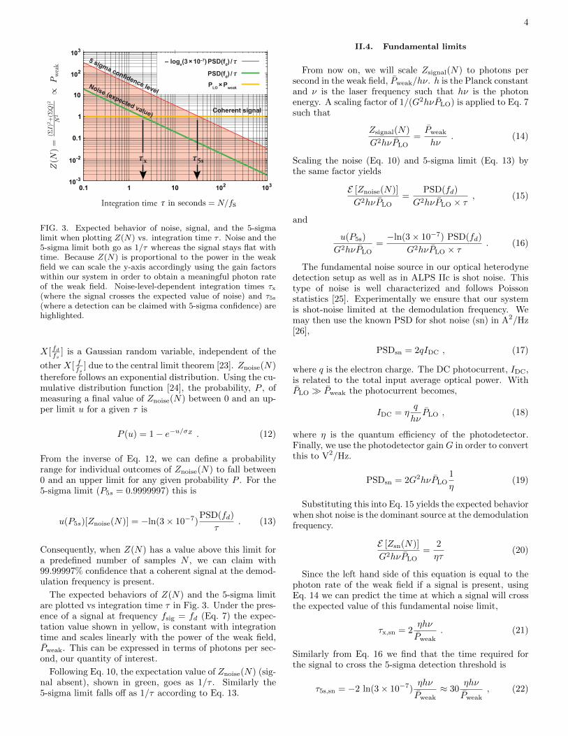
FIG. 3. Expected behavior of noise, signal, and the 5-sigmalimit when plotting Z(N) vs. integration time τ . Noise and the5-sigma limit both go as 1/τ whereas the signal stays flat withtime. Because Z(N) is proportional to the power in the weakfield we can scale the y-axis accordingly using the gain factorswithin our system in order to obtain a meaningful photon rateof the weak field. Noise-level-dependent integration times τx(where the signal crosses the expected value of noise) and τ5s(where a detection can be claimed with 5-sigma confidence) arehighlighted.

X[ fdfs ] is a Gaussian random variable, independent of the

other X[ ffs ] due to the central limit theorem [23]. Znoise(N)

therefore follows an exponential distribution. Using the cu-mulative distribution function [24], the probability, P , ofmeasuring a final value of Znoise(N) between 0 and an up-per limit u for a given τ is

P (u) = 1− e−u/σZ . (12)

From the inverse of Eq. 12, we can define a probabilityrange for individual outcomes of Znoise(N) to fall between0 and an upper limit for any given probability P . For the5-sigma limit (P5s = 0.9999997) this is

u(P5s)[Znoise(N)] = −ln(3× 10−7)PSD(fd)

τ. (13)

Consequently, when Z(N) has a value above this limit fora predefined number of samples N , we can claim with99.99997% confidence that a coherent signal at the demod-ulation frequency is present.

The expected behaviors of Z(N) and the 5-sigma limitare plotted vs integration time τ in Fig. 3. Under the pres-ence of a signal at frequency fsig = fd (Eq. 7) the expec-tation value shown in yellow, is constant with integrationtime and scales linearly with the power of the weak field,Pweak. This can be expressed in terms of photons per sec-ond, our quantity of interest.

Following Eq. 10, the expectation value of Znoise(N) (sig-nal absent), shown in green, goes as 1/τ . Similarly the5-sigma limit falls off as 1/τ according to Eq. 13.

II.4. Fundamental limits

From now on, we will scale Zsignal(N) to photons persecond in the weak field, Pweak/hν. h is the Planck constantand ν is the laser frequency such that hν is the photonenergy. A scaling factor of 1/(G2hνPLO) is applied to Eq. 7such that

Zsignal(N)

G2hνPLO=Pweak

hν. (14)

Scaling the noise (Eq. 10) and 5-sigma limit (Eq. 13) bythe same factor yields

E [Znoise(N)]

G2hνPLO=

PSD(fd)

G2hνPLO × τ, (15)

and

u(P5s)

G2hνPLO=−ln(3× 10−7) PSD(fd)

G2hνPLO × τ. (16)

The fundamental noise source in our optical heterodynedetection setup as well as in ALPS IIc is shot noise. Thistype of noise is well characterized and follows Poissonstatistics [25]. Experimentally we ensure that our systemis shot-noise limited at the demodulation frequency. Wemay then use the known PSD for shot noise (sn) in A2/Hz[26],

PSDsn = 2qIDC , (17)

where q is the electron charge. The DC photocurrent, IDC,is related to the total input average optical power. WithPLO � Pweak the photocurrent becomes,

IDC = ηq

hνPLO , (18)

where η is the quantum efficiency of the photodetector.Finally, we use the photodetector gain G in order to convertthis to V2/Hz.

PSDsn = 2G2hνPLO1

η(19)

Substituting this into Eq. 15 yields the expected behaviorwhen shot noise is the dominant source at the demodulationfrequency.

E [Zsn(N)]

G2hνPLO=

2

ητ(20)

Since the left hand side of this equation is equal to thephoton rate of the weak field if a signal is present, usingEq. 14 we can predict the time at which a signal will crossthe expected value of this fundamental noise limit,

τx,sn = 2ηhν

Pweak. (21)

Similarly from Eq. 16 we find that the time required forthe signal to cross the 5-sigma detection threshold is

τ5s,sn = −2 ln(3× 10−7)ηhν

Pweak≈ 30

ηhν

Pweak, (22)

5

in the case of a shot-noise limited input signal.In conclusion, for a weak field with a power equivalent

to 1 photon per second it takes 2 seconds for the expectedvalue of shot noise to decrease to the signal level. However,it takes ≈ 30 seconds in order to claim a detection of a sig-nal with 5-sigma confidence. For arbitrary noise input bothintegration times, as depicted in Fig. 3, can be generalizedto

τx =PSD(fd)

G2× 1

PLOPweak, (23)

and

τ5s =PSD(fd)

G2×−ln

(3× 10−7

)PLOPweak

, (24)

if the noise is locally flat around fd. The factor betweenτ5s and τx

τ5sτx

= − ln(3× 10−7

)≈ 15 , (25)

does not depend on the PSD, the average power of eitherlaser, or the sampling frequency fs.

Additionally, Eq. 23 shows the importance of a higherpower PLO when the system is not dominated by shot noise.The larger the LO power, the less time required for thesignal to cross the expected noise limit, thus improvingthe SNR. However, once PLO is large enough such that thesystem is shot-noise limited, τx and, consequently, the SNRno longer depend on the LO power.

III. EXPERIMENTAL SETUP

III.1. Optical Design

To demonstrate this concept experimentally, we assem-bled the optical setup shown in Fig .4. This apparatus al-lows us to measure the resultant beat note generated frominterfering a weak field with our LO. There are two 1064nm lasers used. L1 is our LO and L2 provides the fieldused for weak signal generation. A half-wave plate and po-larizing beam splitter (PolBS) pair is placed at the start ofeach beam path for power control purposes. This combina-tion also causes the outgoing light to be linearly polarized.Laser 2 passes through an electro-optic modulator (EOM)which generates sidebands to be used as the weak signal.This will be discussed in more detail later in this section.Laser 2 then passes through two neutral density (ND) fil-ters with a combined attenuation factor of 105 in order tofurther reduce the weak-field signal to an appropriate level.

The two fields are interfered at a power beam splitter(BS) and the combined beam is sent into a single-modepolarization-maintaining fiber. By sending both beamsinto the same single-mode fiber we ensure complete overlapof the spatial eigenmodes at the output coupler. After thefiber, the combined beam passes through another BS. Eachpath is then focused individually onto separate photode-tectors. PD1 is used to lock the two lasers to the constantdifference frequency. This is done via feedback to the lasercontroller for L1 using a phase lock loop (PLL) setup. PD2

BS

PM Fiber

Mirror

Servo Loop

Laser 1 Laser 2

PDI

λ/2λ/2

λ/2

λ/2

BS

PolBS

PolBS

EOM

to DataAcquisition

PD1

PD2

sin(2π fcc t)

sin(2π fEOM t)

ND

FIG. 4. Optical layout of the heterodyne interferometer used forsingle photon detection. Each laser separately passes througha half wave plate and polarizing beam splitter pair for powercontrol purposes and to guarantee linear polarization. L2 issent through an electro-optic modulator driven with a functiongenerator at frequency fEOM. The two beams are then inter-fered at a power beam splitter and sent into a fiber to ensurecomplete spatial overlap. The combined beam at the output ofthe fiber passes through another power beam splitter and eachpath is separately incident onto one of two photodetectors. Onephotodetector is used to phase lock the two lasers via a feed-back loop using mixing with a sine wave generated by an NCOat frequency fCC. The second photodetector is used for theweak-field measurements.

is a homemade photodetector used for our signal measure-ments. For a large enough local oscillator power the shotnoise level exceeds the noise equivalent power (NEP) of thephotodetector and PD2 produces shot-noise limited signals.We set the average local oscillator power to 5 mW and ob-serve a shot noise to NEP ratio of 6 at the measurementfrequency.

Overlapping the two lasers generates a beat note betweenL1 and L2, called the carrier-carrier (CC) beat note at fre-quency fCC. The error signal for the PLL feedback comesfrom mixing the carrier-carrier beat note with a numer-ically controlled oscillator (NCO), also at frequency fCC,synchronized to a master clock. This feedback is controlledby the FPGA card and keeps the CC beat note stable atfrequency fCC.

III.2. Digital Design

The electrical signal from PD2 is digitized via an ADCon-board a FPGA card at a rate of fs = 64 MHz. A simpli-fied digital layout following the path of the photodetectorsignal is detailed in Fig. 5.

The signal at frequency fsig is mixed down to an inter-mediate frequency, fδ, on the order of a few Hz. This isdone via multiplication with a sinusoid from an NCO atfrequency f1 = fsig − fδ generated with a look-up table onthe FPGA card.

While it is possible to directly demodulate down to DCduring the first demodulation simply by setting the NCOfrequency to f1 = fsig, when tested, we observed spuriousDC signals generated within the FPGA card. The strengthof these signals are orders of magnitude larger than the beatnotes of interest thus preventing any useful measurements.This issue is solved by mixing the beat note signal downto the intermediate frequency, writing the data to file, and

6

FPGA

Data Processing (20 Hz)Data Acquisition (64 MHz)

fromOptical Setup

PD2

∑

∑

ADC

CIC Filter

1 х sin(2π f1 / fs n)

A х sin(2π fsig / fs n)

1 х sin(2π f2/ fs' n')

1 х cos(2π f2 / fs' n')

NCO

FIG. 5. Digital layout of detection scheme describing the dig-ital processing techniques involved. The photodetector signalis digitized via an analog-to-digital converter at a rate of 64MHz after which it is mixed with a sine wave, produced by anumerically controlled oscillator, at frequency f1. A cascadedintegrated comb filter is used to remove the higher frequencycomponents due to mixing and downsample the data to 20 Hz,where is it written to file. f ′s and n′ are used to reference thelower sampling rate. I/Q demodulation is done onboard a desk-top computer, and the quadratures are individually summedand Z(N) is computed.

performing a second demodulation stage on a desktop PC.This shifts the unwanted spurious signal to a non-zero fre-quency where it integrates away. With this configuration,the beat note can be accurately measured.

A cascaded integrated comb (CIC) filter [27], removesthe higher frequency components resulting from the mixingprocess. The CIC filter also downsamples the data to a rateof f ′s ≈ 20 Hz at which it is written to file.

The signal at fδ is then decomposed into its in-phase (I)and quadrature (Q) components via separate mixing with acosine and sine NCO at f2 = fδ, respectively. Consideringthe same signal input from Eq. 2 this process referenced tothe higher sampling rate, fs, is equivalent to:

I2[n] = xsig[n] sin (2πf1fsn)× cos (2π

f2fsn)

Q2[n] = xsig[n] sin (2πf1fsn)× sin (2π

f2fsn) .

(26)

The DFT of the recorded data at the lower sampling rate,|X[ f2f ′

s]|2, is then computed. The expectation values of

Z(N) from Section II must be rewritten to include this sec-ond demodulation stage. We denote these equations witha subscript 2. The total number of samples written to fileis denoted N ′ = τf ′s.

With a signal present at the demodulation frequency inthe absence of noise we find

Z2,sig(N ′) =G2

4PLOPweak . (27)

Solving for the photon rate in the weak field,

4 Z2,sig(N ′)

G2hνPLO=Pweak

hν. (28)

Using this new scaling factor of 4/(G2hνPLO), we obtaina quantity equal to the photon rate of the weak field aftertwo demodulation stages.

In the case where there is only noise at the input, thePSD when the data are recorded (DPSD′) must be relatedto the original DPSD right after the ADC. Multiplicationby a sine wave reduces the DPSD by a factor of 2. Thedecimation stage reduces the level of the DPSD by a factor

off ′s

fs. For |f2| ≤ f ′

s

2 ,

DPSD′(f2f ′s

)=

1

2

f ′sfs

DPSD

(fdfs

)=f ′s2

PSD(fd) . (29)

This is related to the DFT by,

DPSD′(f2f ′s

)= E

{|X[ f2f ′

s]|2

N ′

}= E{Z2(N ′)×N ′} . (30)

Solving for E [Z2(N ′)] in terms of the analog PSD evaluatedat fd = f1 + f2 gives

E [Z2,noise(N′)] =

PSD(fd)

2τ, (31)

where we use the substitution N ′ = τf ′s. In order to com-pare the expectation value of noise to that of the signal, wemust apply the new scaling factor of 4/(G2hνPLO). Doingso, we arrive at

4 E [Z2,noise(N′)]

G2hνPLO=

2 PSD(fd)

G2hνPLO × τ. (32)

For the shot-noise limited case with PSDsn given by Eq. 19,this yields

4 E [Z2,sn(N ′)]

G2hνPLO=

4

ητ. (33)

Comparing to Eq. 20, the introduction of a second demod-ulation stage causes the sensitivity to decrease by a factorof 2. This, in turn, also causes the 5-sigma limit to increaseby a factor of 2. Therefore, using two demodulation stagesrequires twice as long an integration time (when comparedto a single stage setup) to confidently detect a signal.2

Signal and noise add linearly in the PSD:

4 E [Z2,total(N′)]

G2hνPLO=Pweak

hν+

4

ητ. (34)

For short integration times and a low photon rate, 4/ητis the dominating term. After long enough integration,Pweak/hν becomes dominant causing the curve to remainconstant with time.

These equations now reflect the result of a second de-modulation stage, however, one final experimental consid-eration must be taken into account. Simply lowering Pweak

2 In principle, it is possible to regain the earlier sensitivity while stillusing two demodulation stages. This is done by taking both I and Qout of the FPGA. Then a second I/Q demodulation is performedon each output channel. This results in four terms II’, IQ’, QI’,and QQ’ where the prime indicates the second demodulation stage.Using a specific combination of these terms yields the same set ofequations described in Section II [28]. This concept is currentlybeing tested and has not yet been implemented.

7

to sub-photon per second levels reduces the CC beat notebelow the point at which the PLL becomes unstable. Ex-perimentally, a stable lock can be maintained with PLO = 5mW and Pweak = 60 pW measured at PD1. This leads toa minimum CC beat note amplitude on the order of 1 µW,equivalent to 3× 108 photons per second in the weak field.Increasing PLO any further pushes the photodetector pastthe level at which it begins to saturate. Therefore, the min-imum photon rate of Laser 2 at PD2, such that the PLLremains stable, is 3× 108 photons per second. In order togenerate signals with field strengths below this value, whilestill maintaining a stable PLL between the two lasers, wemake use of phase modulation from an EOM.

III.3. EOM Sideband Generation

As mentioned earlier, the EOM shown in Fig. 4 was usedto generate sidebands on Laser 2. The EOM is driven atfrequency fEOM using a sine wave from a function gener-ator that is synchronized to a maser clock. This phasemodulates the beam as it passes through the EOM. Phasemodulation generates sidebands both above and below thelaser frequency. These sidebands occur at k integer mul-tiples of the drive frequency, fEOM. The amount of lightpower in the kth order sideband is given by [29]

PSB,k = Jk(m)2Pweak , (35)

where Jk(m) is the kth order Bessel function and m is themodulation depth, dependent on the drive amplitude ofthe modulation. All of these sidebands beat with the LOto produce AC signals with peak amplitudes given by thefollowing,

Ak = 2√PSB,k PLO . (36)

The two ND filters directly after the EOM attenuate thepower of Laser 2 and all of the subsequent sidebands by afactor of 105. The addition of these ND filters is necessaryto reduce the sideband power of interest to the desired level.

The power in the kth sideband, PSB,k, can be fine tunedby adjusting the drive amplitude to the EOM, thus chang-ing the modulation depth, m. To set the modulation depthto a specific value, the two ND filters are removed suchthat both the CC and sideband beat notes are visible ona spectrum analyzer. The ratio between the two beat noteamplitudes is adjusted in order to obtain the desired mod-ulation depth. The ND filters are then placed back intothe beam path. Since the filters are placed after the EOM,the modulation depth remains unchanged.

Using this configuration, the average power of Laser 2 isset to maintain a stable PLL. Higher order sidebands falloff in power to levels comparable to the expected sensitivityof ALPS IIc. The interference between these sidebands andthe LO form beat notes at known, fixed frequencies.

IV. RESULTS

IV.1. Noise Behavior and Device Sensitivity

We first performed a measurement with no weak signalpresent to study the behavior of the noise in our system.Only the LO beam with power PLO = 5 mW is incidentonto PD2. At 5 mW, the photodetector is shot-noise lim-ited. The photodetector has gain G = 1.44 × 103 V/Wand quantum efficiency η = 0.7. After both demodula-tion stages, Z2(N ′) is computed and the result is scaled toan equivalent photon rate using the factor stated in Eq. 33.The result of this 19 day long measurement, plotted againstintegration time τ , is shown in Fig. 6.

τIntegration time

5 sigma confidence levelExpected value

Measurement data (2.5 Hz)50 run average (2.5-3.0 Hz)Double demodulation limit

Shot noise limit

FIG. 6. Shot-noise limited measurement with no weak signalpresent. After second demodulation at f2 = 2.5 Hz, Z2(N ′) iscomputed and the resultant is scaled to an equivalent photonrate, shown in yellow. Z2(N ′) is also computed for 50 separatedemodulation frequencies near 2.5 Hz. These are then averagedto produce the dark blue line. This average follows the expectedvalue line, shown in red, based on the PSD of the noise. Thepurple line shows the 5-sigma limit that the measurement curvewould cross if a signal was present. The fundamental shot-noiselimit (if only one demodulation stage was required) is drawnin light blue for comparison. The second demodulation stageincreases the shot-noise limit by a factor of 2 (dashed green).Because the expected value of the measurement sits on top ofthis theoretical limit we show that shot noise is the dominantnoise source in our setup.

Z2(N ′) was computed 50 additional times using differentdemodulation frequencies near 2.5 Hz. The results are thenscaled to the photon rate and averaged. This average isidentical to the curve representing the expectation valuesfor different integration times. Both have essentially thesame amplitude and fall off as 1/τ as expected. The datastream demodulated at 2.5 Hz shows one representation ofa shot noise dominated signal over the integration time. Inaddition, the 5-sigma threshold is plotted.

The light blue line shows the expected fundamental shot-noise limit for the given optical power if only one demodu-lation stage was used. As our measurement requires a sec-ond demodulation stage, the amount of shot noise, scaled

8

to photons per second, increases by a factor of 2 (Eq. 33),shown as the dashed green line. Since the expectation valueof our data lies on top of the theoretical shot-noise limit af-ter the second demodulation stage, shot noise is in fact thedominant noise source in our setup.

This measurement verifies that our system is shot-noiselimited and behaves as expected. Because the measurementdoes not cross the 5-sigma threshold, this also shows thatno spurious signals are picked up over the entire 19 dayintegration time when Laser 2 was turned off.

IV.2. Weak Signal Generation and Detection

In order to demonstrate that a signal is observable usingheterodyne detection, we generate a beat note between theLO and an ultra-weak sideband of the second laser. Wechoose a sideband power equivalent to ≈ 10−2 photons persecond. Reducing the signal further was not possible inour current setup as we started to pick up spurious sig-nals electronically. While this has been observed we wantto stress that the spurious signal vanishes when the EOMphase modulation is turned off. Thus, it is not an artifactof the second laser field but rather a result of the modula-tion itself. We assume the issue to be cross-talk betweenthe function generator driving the EOM and the FPGAdata acquisition and signal processing card. Further workon generating ultra-weak laser fields without electrical in-terference is required.

In order to generate a sideband with the specified power,we first remove the ND filters and set the local oscillatorto PLO = 5 mW and L2 to PL2 = 6 µW. Both of thesemeasurements are taken at the photodetector input. Themodulation depth is set to m = 0.0109 by adjusting thedrive amplitude to the EOM. Using Eq. 35, the power inthe 2nd order sideband (k = +2) is calculated to be onthe order of 10−15 W. The ND filters are placed back intothe beam path attenuating the sideband by a factor of 105,yielding PSB,2 = 6.33× 10−21 W. For 1064 nm light, this isequivalent to 3.39 × 10−2 photons per second in the side-band we wish to measure.

The CC beat note between L1 and L2 is set to 30 MHz.Phase modulation is done by driving the EOM with a sinewave at 23 MHz + 1.2 Hz. This sets the beat note betweenthe 2nd order sideband and L1 to be at fsig = 16 MHz+ 2.4 Hz. With the first demodulation frequency set tof1 = 16 MHz, the beat note of interest is therefore at 2.4Hz when the data are written to file. These data are thenimported into MATLAB where the second demodulationis performed. Finally, we compute Z2(N ′) and scale theresult to photons per second.

The results of this measurement are shown in Fig. 7.Demodulating at a frequency not equal to any signal fre-quency demonstrates the expected behavior of noise. Thisis shown by the amber curve for which a demodulation 0.1Hz away from the 2.4 Hz signal was used. In this case,no coherent signal can accumulate and the only influenceat the demodulation frequency is noise. This matches thetrend of the expectation value of the noise, shown in red.

Demodulating at the signal frequency of 2.4 Hz, shownin blue, initially behaves as noise. This continues until the

τIntegration time

Signal present at 2.4 Hz5 sigma detection limit

3.33 x 10-2 photonsper second

Demodulation at exactly 2.4 HzDemodulation at 2.4003 Hz

Demodulation 2.5 HzExpected value (no signal)

FIG. 7. Shot-noise limited signal measurement scaled to pho-tons per second. Two demodulation stages are used with a sig-nal present at 2.4 Hz when the data are written to file. Whensecond demodulation is at a frequency f2 6= 2.4 Hz, the resultyields the behavior of noise, shown in yellow. The trend of theexpectation value for this level of noise is shown in red. The5-sigma confidence line is shown in purple. The result whendemodulating at the signal frequency, f2 = 2.4 Hz is shown inlight blue. This curve crosses the 5-sigma line, demonstrating aconfident detection. The level that this flattens out to yields arate in the sideband of interest of 3.33× 10−2 photon/s, shownin dark blue. Demodulating at a frequency 300 µHz away fromthe signal, shown in green, highlights the energy resolution ofthis detection method.

signal begins to dominate, causing the curve to flatten outand subsequently cross the 5-sigma threshold. The level atwhich this curve flattens out yields a rate for the sidebandof 3.33 × 10−2 photons/s. The measured photon rate iswithin the range of error of 6%. This error arises from bothlaser power measurements and modulation depth measure-ments. The constant level crosses the red expected noisecurve at ≈ 120 seconds, in agreement with the expected τx.A 5-sigma confidence detection is made after ≈ 1800 sec-onds of integration time, in agreement with the expectedτ5s. We therefore demonstrate that our experimental setupis viable for both generating and detecting sub-photon persecond level signals using optical heterodyne interferome-try.

Demodulation 300 µHz away from the signal demon-strates the importance of maintaining phase coherencethroughout the entire measurement. In this case, shownin green, the demodulation waveform drifts in and out ofphase with the signal. When this happens, the integratedI and Q values begin to oscillate with the difference fre-quency (fsig − fd). This causes Z2(N ′) to fall off as a sincfunction, preventing it from crossing the 5-sigma threshold.

V. CONCLUSION

These measurements demonstrate that heterodyne inter-ferometry can be applied as a single photon detector. Ithowever requires that the demodulation waveform main-

9

tains phase coherence with the signal during the entire in-tegration time. Measurements at the shot-noise limit withLaser 2 off did not reveal any spurious signals that woulddegrade the sensitivity of our setup after 19 days of integra-tion. Therefore we can confidently detect coherent signalswith field strengths equivalent to 10−6 photons per second.

We also demonstrate successful generation and detectionof a signal with a field strength on the order of 10−2 pho-tons per second. Longer integration times and improve-ments in the generation of ultra-weak laser fields are re-quired to achieve low power levels which are comparable tothe expected sensitivity of ALPS IIc. Work on the genera-tion, implementation, and detection of weaker signal fieldsis currently ongoing.

Our results also highlight the importance of maintain-ing phase coherence and stability throughout the measure-ment. These limitations to heterodyne detection must betaken into account during implementation into ALPS II.

While this detection method emerged from the need of asingle photon detector for the ALPS II experiment, hetero-

dyne interferometric detection of weak fields can be modi-fied for a variety of applications. Although this techniqueis demonstrated here using 1064 nm laser light, it can beextended to any wavelength provided that noise and thecoherent signal can be decoupled. The versatility of het-erodyne detection makes it applicable to a broad range offields including astronomy, classical communications, andbiomedical imaging [30], as long as the signal is coherentand its frequency is known.

VI. ACKNOWLEDGEMENTS

The authors would like to thank Johannes Eichholz forthe phase meter design used for real time signal demodu-lation. This material is based upon work supported by theNational Science Foundation under Grant No. 1505743 andthe Heising-Simons Foundation under Grant No. 2015-154.

[1] Baker et al., Phys. Rev. Lett. 97, 131801 (2006).[2] R. D. Peccei and H. R. Quinn, Phys. Rev. Lett. 38, 1440

(1977).[3] S. Weinberg, Phys. Rev. Lett. 40, 223 (1978).[4] F. Wilczek, Phys. Rev. Lett. 40, 279 (1978).[5] K. Olive and P. D. Group, Chinese Physics C 38 (2014).[6] P. Svrcek and E. Witten, Journal of High Energy Physics

2006, 051 (2006).[7] P. W. Graham, I. G. Irastorza, S. K. Lamoreaux, A. Lind-

ner, and K. A. van Bibber, Annual Review of Nuclear andParticle Science 65, 485 (2015).

[8] M. Meyer, D. Horns, and M. Raue, Phys. Rev. D 87,035027 (2013).

[9] J. I. S. Catalan, E. Garcıa-Berro, and S. Torres, The As-trophysical Journal Letters 682, L109 (2008).

[10] P. Sikivie, Phys. Rev. Lett. 51, 1415 (1983).[11] H. Primakoff, Phys. Rev. 81, 899 (1951).[12] Asztalos et al., Phys. Rev. Lett. 104, 041301 (2010).[13] K. e. a. Zioutas (CAST Collaboration), Phys. Rev. Lett.

94, 121301 (2005).[14] K. Van Bibber, N. R. Dagdeviren, S. E. Koonin, A. K. Ker-

man, and H. N. Nelson, Phys. Rev. Lett. 59, 759 (1987).[15] F. Hoogeveen and T. Ziegenhagen, Nuclear Physics B 358,

3 (1991).[16] Yukio Fukuda and Toshiro Kohmoto and Shin-ichi Naka-

jima and Masakuzu Kunitomo, Progress in Crystal Growthand Characterization of Materials 33, 363 (1996).

[17] Ehret et al., Nuclear Instruments and Methods in PhysicsResearch Section A: Accelerators, Spectrometers, Detectorsand Associated Equipment 612, 83 (2009).

[18] G. Mueller, P. Sikivie, D. B. Tanner, and K. van Bibber,Phys. Rev. D 80, 072004 (2009).

[19] R Bahre et al., Journal of Instrumentation 8, T09001(2013).

[20] Aaron D. Spector and Jan H. Pold and Robin Bahre andAxel Lindner and Benno Willke, Opt. Express 24, 29237(2016).

[21] Dreyling-Eschweiler et al., Journal of Modern Optics 62,1132 (2015).

[22] P. Stoica and R. L. Moses, Spectral analysis of signals(Pearson/Prentice Hall, 2005).

[23] M. Peligrad and W. B. Wu, Ann. Probab. 38, 2009 (2010).[24] A. Papoulis and S. Pillai, Probability, random variables,

and stochastic processes, McGraw-Hill electrical and elec-tronic engineering series (McGraw-Hill, 2002).

[25] M. Fox, Quantum Optics: An Introduction (Oxford masterseries in physics ; 6) (Oxford University Press, 2006).

[26] P. M. Mayer, F. Rana, and R. J. Ram, Applied PhysicsLetters 82, 689 (2003).

[27] E. Hogenauer, IEEE Trans. Acoust., Speech, Signal Pro-cessing 29, 155 (1981).

[28] E. Ragaini and R. F. Woodman, Radio Science 32, 783.[29] B. Saleh and M. Teich, Fundamentals of Photonics, Wiley

Series in Pure and Applied Optics (Wiley, 2013).[30] R. H. Hadfield, Nature Photonics 3, 696 (2009).