Single image object modeling based on BRDF and r-surfaces learning

Fabrizio Natola, Valsamis Ntouskos, Fiora Pirri, Marta Sanzari

ALCOR Lab, DIAG, Sapienza University of Rome

natola,ntouskos,pirri,sanzari@diag.uniroma1.it

Abstract

A methodology for 3D surface modeling from a single

image is proposed. The principal novelty is concave and

specular surface modeling without any externally imposed

prior. The main idea of the method is to use BRDFs and

generated rendered surfaces, to transfer the normal field,

computed for the generated samples, to the unknown sur-

face. The transferred information is adequate to blow and

sculpt the segmented image mask in to a bas-relief of the

object. The object surface is further refined basing on a

photo-consistency formulation that relates for error mini-

mization the original image and the modeled object.

1. Introduction

There is an increasing need for 3D models of objects,

from single images, for several applications such as digi-

tal archives of heritage and monuments, anatomy models

for pathology detection, small artifacts models for populat-

ing rendered 3D scenes with objects or augmenting a MO-

CAP sequence with tools for manipulation and, finally, for

robotics. Likewise, there is a growing awareness that 3D

modeling, from a single image, helps to navigate the sea of

terabytes of images, for the object recognition challenge.

That surface modeling from a single view has to deal

with shading and the way materials shine and reflect the

light has become clear since the works of [31] and [20].

Though only recently a great deal of work has been done to

merge the rich information that light conveys about an ob-

ject with its shape. Relevant examples are studies on specu-

lar reflection of materials and light incidence [23, 24], so as

to dismiss the Lambertian hypothesis, and on how illumi-

nation and reflectance combine to influence an object shape

perception [4] and its geometry [34].

Here, we address these problems introducing a novel

method, which is unbiased to the changes of the ambient

light, taking care of both concavities and sharp parts of an

object, this is the main contribution of this paper. Our ap-

proach is related to SIRFS [4], who introduced priors for

shape, albedo and illumination, respectively, so as to learn

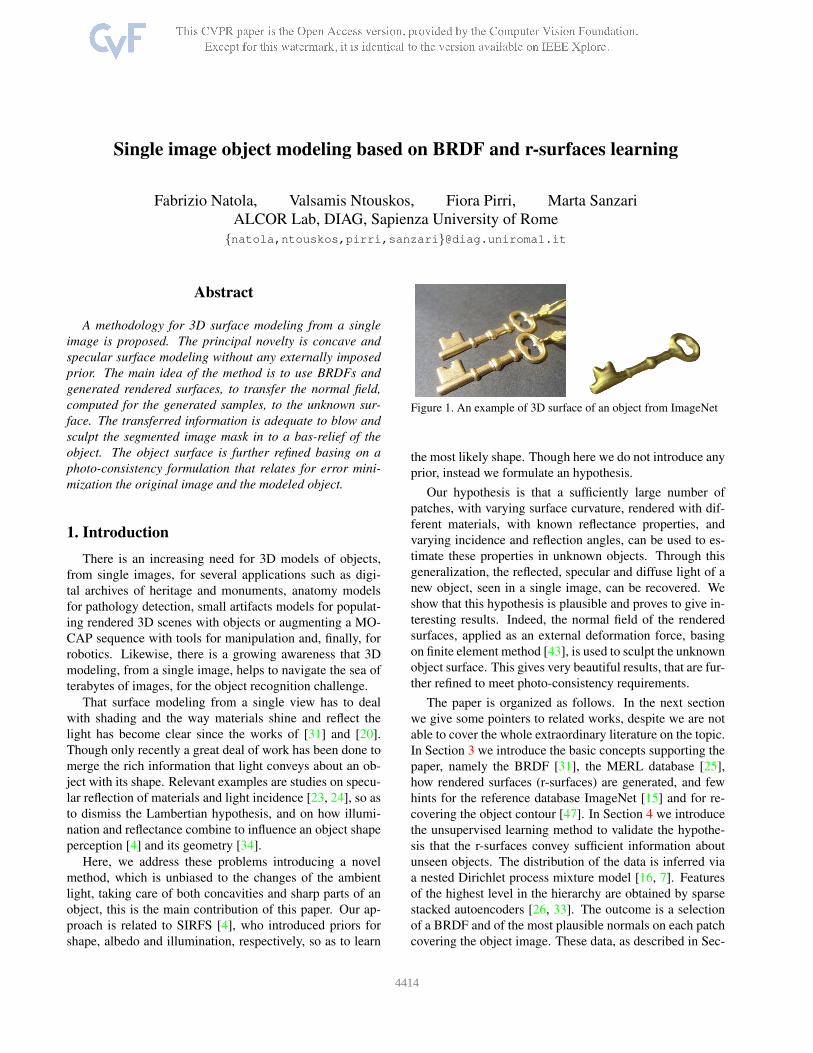
Figure 1. An example of 3D surface of an object from ImageNet

the most likely shape. Though here we do not introduce any

prior, instead we formulate an hypothesis.

Our hypothesis is that a sufficiently large number of

patches, with varying surface curvature, rendered with dif-

ferent materials, with known reflectance properties, and

varying incidence and reflection angles, can be used to es-

timate these properties in unknown objects. Through this

generalization, the reflected, specular and diffuse light of a

new object, seen in a single image, can be recovered. We

show that this hypothesis is plausible and proves to give in-

teresting results. Indeed, the normal field of the rendered

surfaces, applied as an external deformation force, basing

on finite element method [43], is used to sculpt the unknown

object surface. This gives very beautiful results, that are fur-

ther refined to meet photo-consistency requirements.

The paper is organized as follows. In the next section

we give some pointers to related works, despite we are not

able to cover the whole extraordinary literature on the topic.

In Section 3 we introduce the basic concepts supporting the

paper, namely the BRDF [31], the MERL database [25],

how rendered surfaces (r-surfaces) are generated, and few

hints for the reference database ImageNet [15] and for re-

covering the object contour [47]. In Section 4 we introduce

the unsupervised learning method to validate the hypothe-

sis that the r-surfaces convey sufficient information about

unseen objects. The distribution of the data is inferred via

a nested Dirichlet process mixture model [16, 7]. Features

of the highest level in the hierarchy are obtained by sparse

stacked autoencoders [26, 33]. The outcome is a selection

of a BRDF and of the most plausible normals on each patch

covering the object image. These data, as described in Sec-

14414

tion 5, form the external forces of the energy, which deforms

the planar patches, covering the object mask, into the object

surface. This extends the deformation method [45] to con-

cavities and sharp object parts. Finally, the resulting surface

model is made consistent with the object appearance in the

image, by revising the light effects, as described in Section

6. This is obtained with a rich energy term taking care of

both photo-consistency and surface depth, optimized via to-

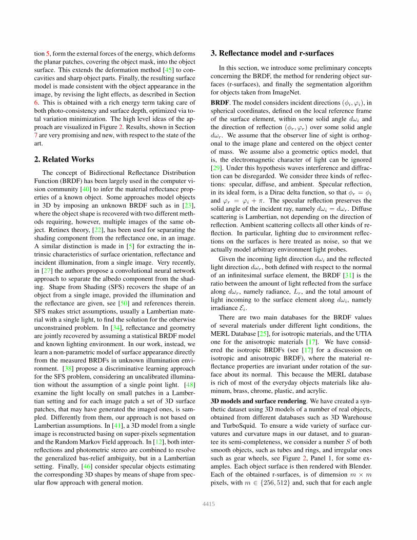
tal variation minimization. The high level ideas of the ap-

proach are visualized in Figure 2. Results, shown in Section

7 are very promising and new, with respect to the state of the

art.

2. Related Works

The concept of Bidirectional Reflectance Distribution

Function (BRDF) has been largely used in the computer vi-

sion community [40] to infer the material reflectance prop-

erties of a known object. Some approaches model objects

in 3D by imposing an unknown BRDF such as in [23],

where the object shape is recovered with two different meth-

ods requiring, however, multiple images of the same ob-

ject. Retinex theory, [22], has been used for separating the

shading component from the reflectance one, in an image.

A similar distinction is made in [5] for extracting the in-

trinsic characteristics of surface orientation, reflectance and

incident illumination, from a single image. Very recently,

in [27] the authors propose a convolutional neural network

approach to separate the albedo component from the shad-

ing. Shape from Shading (SFS) recovers the shape of an

object from a single image, provided the illumination and

the reflectance are given, see [50] and references therein.

SFS makes strict assumptions, usually a Lambertian mate-

rial with a single light, to find the solution for the otherwise

unconstrained problem. In [34], reflectance and geometry

are jointly recovered by assuming a statistical BRDF model

and known lighting environment. In our work, instead, we

learn a non-parametric model of surface appearance directly

from the measured BRDFs in unknown illumination envi-

ronment. [38] propose a discriminative learning approach

for the SFS problem, considering an uncalibrated illumina-

tion without the assumption of a single point light. [48]

examine the light locally on small patches in a Lamber-

tian setting and for each image patch a set of 3D surface

patches, that may have generated the imaged ones, is sam-

pled. Differently from them, our approach is not based on

Lambertian assumptions. In [41], a 3D model from a single

image is reconstructed basing on super-pixels segmentation

and the Random Markov Field approach. In [12], both inter-

reflections and photometric stereo are combined to resolve

the generalized bas-relief ambiguity, but in a Lambertian

setting. Finally, [46] consider specular objects estimating

the corresponding 3D shapes by means of shape from spec-

ular flow approach with general motion.

3. Reflectance model and r-surfaces

In this section, we introduce some preliminary concepts

concerning the BRDF, the method for rendering object sur-

faces (r-surfaces), and finally the segmentation algorithm

for objects taken from ImageNet.

BRDF. The model considers incident directions (φi, ϕi), in

spherical coordinates, defined on the local reference frame

of the surface element, within some solid angle dωi and

the direction of reflection (φr, ϕr) over some solid angle

dωr. We assume that the observer line of sight is orthog-

onal to the image plane and centered on the object center

of mass. We assume also a geometric optics model, that

is, the electromagnetic character of light can be ignored

[29]. Under this hypothesis waves interference and diffrac-

tion can be disregarded. We consider three kinds of reflec-

tions: specular, diffuse, and ambient. Specular reflection,

in its ideal form, is a Dirac delta function, so that φr = φi

and ϕr = ϕi + π. The specular reflection preserves the

solid angle of the incident ray, namely dωi = dωr. Diffuse

scattering is Lambertian, not depending on the direction of

reflection. Ambient scattering collects all other kinds of re-

flection. In particular, lighting due to environment reflec-

tions on the surfaces is here treated as noise, so that we

actually model arbitrary environment light probes.

Given the incoming light direction dωi and the reflected

light direction dωr, both defined with respect to the normal

of an infinitesimal surface element, the BRDF [31] is the

ratio between the amount of light reflected from the surface

along dωr, namely radiance, Lr, and the total amount of

light incoming to the surface element along dωi, namely

irradiance Ei.There are two main databases for the BRDF values

of several materials under different light conditions, the

MERL Database [25], for isotropic materials, and the UTIA

one for the anisotropic materials [17]. We have consid-

ered the isotropic BRDFs (see [17] for a discussion on

isotropic and anisotropic BRDF), where the material re-

flectance properties are invariant under rotation of the sur-

face about its normal. This because the MERL database

is rich of most of the everyday objects materials like alu-

minum, brass, chrome, plastic, and acrylic.

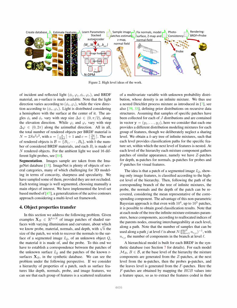
3D models and surface rendering. We have created a syn-

thetic dataset using 3D models of a number of real objects,

obtained from different databases such as 3D Warehouse

and TurboSquid. To ensure a wide variety of surface cur-

vatures and curvature maps in our dataset, and to guaran-

tee its semi-completeness, we consider a number S of both

smooth objects, such as tubes and rings, and irregular ones

such as gear wheels, see Figure 2, Panel 1, for some ex-

amples. Each object surface is then rendered with Blender.

Each of the obtained r-surfaces, is of dimension m × mpixels, with m ∈ 256, 512 and, such that for each angle

4415

Create database Estimate Features Learn Parameters Sample image

patches estimate:

z-map,

normal field

Fix normals, model

surface, Z-map and

normal-field

Photo-

Consistency

Rendering:

BRDF+Probe

Probe

Stacked

autoencoder

in out in out(W ,W ,b ,b )

depth

normals

image features

N-DPM

Figure 2. High level ideas of the work.

of incident and reflected light (φi, ϕi, φr, ϕr), and BRDF

material, an r-surface is made available. Note that the light

direction varies according to (φi, ϕi), while the view direc-

tion according to (φr, ϕr). Light is distributed considering

a hemisphere with the surface at the center of it. The an-

gles φi and φr vary with step size ∆φ ∈ (0, π/2), along

the elevation direction. While ϕi and ϕr vary with step

∆ϕ ∈ (0, 2π) along the azimuthal direction. All in all,

the total number of rendered objects per BRDF material is

N = 2Sa2c2, with a = ⌈ π2∆φ⌉+ 1 and c = ⌈ 2π

∆ϕ⌉. The set

of rendered objects is B = B1, · · · , Bb, with b the num-

ber of considered BRDF materials, and each Bi is made of

N rendered objects. For the ambient light we used 16 dif-

ferent light probes, see [14].

Segmentation. Images sample are taken from the Ima-

geNet database [15]. ImageNet is plenty of objects of sev-

eral categories, many of which challenging for 3D model-

ing in terms of concavity, sharpness and specularity. We

have sampled some of them, provided they are not occluded.

Each testing image is well segmented, choosing manually a

main object of interest. We have implemented the level-set

based method of [47], a generalization of the active contours

approach considering a multi-level set framework.

4. Object properties transfer

In this section we address the following problem. Given

examples XB ∈ Rh×N of image patches of shaded sur-

faces with varying illumination and curvature, about which

we know probe, material, normals, and depth, with√h the

size of the patch, we wish to recover the normals to the sur-

face of a segmented image IQ, of an unknown object Q,

the material it is made of, and the probe. To this end we

have to establish a correspondence between the patches of

the unknown surface IQ and the patches of the known r-

surfaces XB , in the synthetic database. We can see the

problem under the following perspective. If we consider

a hierarchy of properties of a patch, such as surface fea-

tures like depth, normals, probe, and image features, we

can see that each group of features is a scattered realization

of a multivariate variable with unknown probability distri-

bution, whose density is an infinite mixture. We thus use

a nested Dirichlet process mixture as introduced in [7], see

also [39, 35], defining prior distributions on recursive data

structures. Assuming that samples of specific patches have

been collected for each of J distributions and are contained

in vector y = (y1, . . . , yJ), here we consider that each one

provides a different distribution modeling mixtures for each

group of features, though we deliberately neglect a sharing

level. We obtain a k-ary tree of infinite mixtures, such that

each level provides classification paths for the specific fea-

ture set, within which the next level of features is nested. At

each level of the hierarchy each mixture component gathers

patches of similar appearance, namely we have Z-patches

for depth, n-patches for normals, p-patches for probes and

F -patches for visual features.

The idea is that a patch of a segmented image IQ, show-

ing only image features, is classified according to the high-

est level of the hierarchy. Then, following the path of the

corresponding branch of the tree of infinite mixtures, the

probe, the normals and the depth of the patch can be re-

covered, considering the mean representative of the corre-

sponding component. The advantage of this non-parametric

Bayesian approach is that even with 104, up to 105 patches,

it is possible to obtain good classification results. Note that

at each node of the tree the infinite mixture estimates param-

eters, hence components, according to reallocated indices of

the parents nodes, ensuring interchangeability at each level,

along a path. Note that the number of samples that can be

used along a path j at level ℓ is about N(∏jℓ

i=1 ncjℓ)−1, with

ncjℓ the number of components in the branch at level ℓ.

A hierarchical model is built for each BRDF in the syn-

thetic database (see Section 7 for details). For each model

MB , B ∈ B, at the base level of the hierarchy the mixture

components are generated from the Z-patches, at the next

level from the n-patches, then the probes p-patches, and

the leaves level is generated from the F -patches. Here the

F -patches are obtained by mapping the RGB values into

a feature space, so as to extract the features coded in their

4416

representation, ensuring statistical independence of the data

[33, 19]. Autoencoders are a popular computational archi-

tecture to learn features from data [6, 30], here we intro-

duce a sparse stacked autoencoder, to obtain the F -patches

for each BRDF B ∈ B, which determines the features size

from sparsity.

Distribution linking the object image and r-surfaces. Let

Y be a multivariate whose density is an infinite Gaussian

mixture, with unknown parameters. The nested DPM model

we consider is Y |ck,jℓ,θk,jℓ ∼ N (µck,jℓ,Σck,jℓ

), k → ∞and jℓ the level on the path j in the tree. Here ck,jℓ in-

dicates the mixture component k, at level ℓ, on the path jand the θk,jℓ are in turns independently sampled from an

unknown distribution θk,jℓ|Gjℓ ∼ Gjℓ, on which is placed

a Dirichlet process Gjℓ ∼ DP (αℓG0,ℓ). Here αℓ is the

concentration parameter, affecting the number of compo-

nents that will be generated, and G0,ℓ is the base distribu-

tion, typically the conjugate prior of the observation distri-

bution (for the DPM at each level in a path, we refer the

reader to the recent [8, 44] though the models go back to

[16, 2]). Assume, now, that the parameters have been com-

puted for each group of features, that a nested DPMs MB

is obtained for each B ∈ B, actually each with 4 levels.

Each nested DPM has a number of j-paths according to the

recursive structure induced by the groups of features. Given

a nested DPM for each B ∈ B we are concerned with the

computation of the data likelihood for a realization hQB, of

a patch XQ, whose BRDF has been identified to be B (see

below). Once P (cjℓ = kjℓ|hQB,MB), is established for

the leaf components at level ℓ = 4, along the path j then,

going back along the path and picking the mean value of the

nodes in the path, we obtain the most plausible features p-

patch and n-patch matching hQB. Note that when the DPM

is trained, the realizations of Y are the patch features hB

of the XB in the synthetic database. To compute the nested

DPM we have used conjugate priors and an extension of

[21], see also [44, 28].

Stacked sparse autoencoder for each BRDF. Let Ω ⊆ Rh

be the data space, H the feature space, and X ∈ Ω be a

patch. Autoencoders [26, 30] provide a structured represen-

tation of the sample data, by estimating an encoding map

f : Λ × Ω 7→ H , and a decoding map g : H × Λ 7→ Ω.

Features generated by an autoencoder β(B) take values

h = f(Λβ , X) = σ(WinX + bin). Optimization for mini-

mizing the loss function is here obtained by the orthant pro-

jection method [1, 42]. The result of the optimization for

the stacked autoencoder are the parameters Λ(1)β ∪ Λ

(2)β .

The final features for patches XB , for B ∈ B, is hB =

σ(W(2)in h

(1)B + b

(2)1 ⊗ 11×M ), of size k ×M ; here h

(1)B =

σ(W(1)in XB + b

(1)1 ⊗ 11×M ) are the lighter feature values,

and ⊗ is the Kronecker product.

On the other hand, let XQ = (XQ1, . . . , XQK

) ∈ Rh×K

be the K patches of IQ (segmented image of Q). The fea-

ture set for IQ is:

HQ/B =

hQ=σ(W(2)in σ(W

(1)in XQ+b

(1)1 ⊗11×K)+b

(2)1 ⊗11×K)|

(W(2)in ,W

(1)in ,b

(2)1 ,b

(1)1 ) ∈ Λ

(1)β ∪Λ(2)

β , ∀B ∈ B(1)

These features are obtained by evaluating each stacked au-

toencoder β(B), B∈B, at XQ. To choose one, consider

the average features for B∈B: s=1/M∑

∀XBhB . Let

ε(x)=− log(x), be the Burg entropy, then according to [13]

we obtain Bregman divergence to measure similarity be-

tween the object features and s:

XQ ∈ B⋆ if B⋆ = argminB d(XQ, B), with

d(XQ, B)=∑

∀hQ∈HQ/B

(ε(s)−ε(hQ))−∇ε(hQ)(s−hQ)

(2)

This results in a full identification of the specific BRDF Bfor each XQ, as the material of the patch. Once the BRDF

B is chosen, the features hQ are the specific realizations of

the multivariate Y . Hence the nested DPM can be applied,

as gathered in the previous paragraph, in order to obtain the

sought for properties to be transferred to XQ.

5. Bas-relief modeling of objects

In this section we present the method for modeling an

object shape, given the information obtained from the in-

ference, described in Section 4. Accordingly, we are given

a number of patches XQ covering the segmented image of

object Q, the normal field transferred from some XB , and

the position of the top left corner within the domain Ω. Note

that the patches are not overlapping.

Object modeling using normals and curvatures Here

we define a binary mask A⊂R2 for image IQ by the

mapping ν:Ω 7→0, 1. The surface, parametrized by

the function w: A7→R3, where w(u, v) is the vector

[x(u, v), y(u, v), z(u, v)]⊤, is obtained by minimizing an

energy functional G(w). The energy functional G(w) is de-

fined by the first and second fundamental forms [45], and it

embeds surface stretching and bending, plus external forces

F acting on it [32].

To correctly identify the external forces we compute

the mean curvature κ(u, v) for each (u, v)∈A, given the

normal n(u, v) at each point of the surface, as estimated

by the N-DPM, see Section 4. The external forces are

needed to sculpt the surface inflation and are of the form

F (u, v) = sign(κ(u, v))qn(u, v), with q∈R+. The scheme

for finding the solution w(·) is based on the Finite Element

method, as described in [43], applied to the Euler-Lagrange

equations associated to the functional G(w). Furthermore,

we require that each normal to the surface w(u, v) is a unit

vector along wu×wv , with wu,wv the partial derivatives

4417

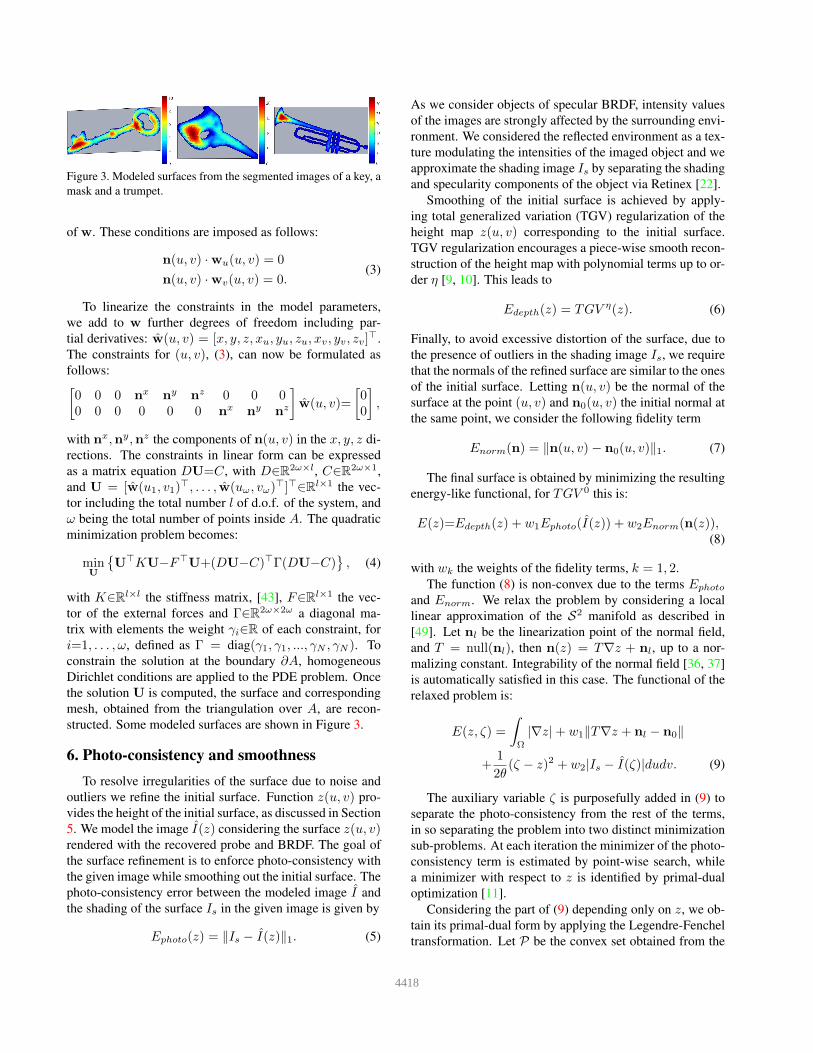
Figure 3. Modeled surfaces from the segmented images of a key, a

mask and a trumpet.

of w. These conditions are imposed as follows:

n(u, v) ·wu(u, v) = 0

n(u, v) ·wv(u, v) = 0.(3)

To linearize the constraints in the model parameters,

we add to w further degrees of freedom including par-

tial derivatives: w(u, v) = [x, y, z, xu, yu, zu, xv, yv, zv]⊤.

The constraints for (u, v), (3), can now be formulated as

follows:[

0 0 0 nx ny nz 0 0 00 0 0 0 0 0 nx ny nz

]

w(u, v)=

[

00

]

,

with nx,ny,nz the components of n(u, v) in the x, y, z di-

rections. The constraints in linear form can be expressed

as a matrix equation DU=C, with D∈R2ω×l, C∈R2ω×1,

and U = [w(u1, v1)⊤, . . . , w(uω, vω)

⊤]⊤∈Rl×1 the vec-

tor including the total number l of d.o.f. of the system, and

ω being the total number of points inside A. The quadratic

minimization problem becomes:

minU

U⊤KU−F⊤U+(DU−C)⊤Γ(DU−C)

, (4)

with K∈Rl×l the stiffness matrix, [43], F∈Rl×1 the vec-

tor of the external forces and Γ∈R2ω×2ω a diagonal ma-

trix with elements the weight γi∈R of each constraint, for

i=1, . . . , ω, defined as Γ = diag(γ1, γ1, ..., γN , γN ). To

constrain the solution at the boundary ∂A, homogeneous

Dirichlet conditions are applied to the PDE problem. Once

the solution U is computed, the surface and corresponding

mesh, obtained from the triangulation over A, are recon-

structed. Some modeled surfaces are shown in Figure 3.

6. Photo-consistency and smoothness

To resolve irregularities of the surface due to noise and

outliers we refine the initial surface. Function z(u, v) pro-

vides the height of the initial surface, as discussed in Section

5. We model the image I(z) considering the surface z(u, v)rendered with the recovered probe and BRDF. The goal of

the surface refinement is to enforce photo-consistency with

the given image while smoothing out the initial surface. The

photo-consistency error between the modeled image I and

the shading of the surface Is in the given image is given by

Ephoto(z) = ‖Is − I(z)‖1. (5)

As we consider objects of specular BRDF, intensity values

of the images are strongly affected by the surrounding envi-

ronment. We considered the reflected environment as a tex-

ture modulating the intensities of the imaged object and we

approximate the shading image Is by separating the shading

and specularity components of the object via Retinex [22].

Smoothing of the initial surface is achieved by apply-

ing total generalized variation (TGV) regularization of the

height map z(u, v) corresponding to the initial surface.

TGV regularization encourages a piece-wise smooth recon-

struction of the height map with polynomial terms up to or-

der η [9, 10]. This leads to

Edepth(z) = TGV η(z). (6)

Finally, to avoid excessive distortion of the surface, due to

the presence of outliers in the shading image Is, we require

that the normals of the refined surface are similar to the ones

of the initial surface. Letting n(u, v) be the normal of the

surface at the point (u, v) and n0(u, v) the initial normal at

the same point, we consider the following fidelity term

Enorm(n) = ‖n(u, v)− n0(u, v)‖1. (7)

The final surface is obtained by minimizing the resulting

energy-like functional, for TGV 0 this is:

E(z)=Edepth(z) + w1Ephoto(I(z)) + w2Enorm(n(z)),(8)

with wk the weights of the fidelity terms, k = 1, 2.

The function (8) is non-convex due to the terms Ephoto

and Enorm. We relax the problem by considering a local

linear approximation of the S2 manifold as described in

[49]. Let nl be the linearization point of the normal field,

and T = null(nl), then n(z) = T∇z + nl, up to a nor-

malizing constant. Integrability of the normal field [36, 37]

is automatically satisfied in this case. The functional of the

relaxed problem is:

E(z, ζ) =

∫

Ω

|∇z|+ w1‖T∇z + nl − n0‖

+1

2θ(ζ − z)2 + w2|Is − I(ζ)|dudv. (9)

The auxiliary variable ζ is purposefully added in (9) to

separate the photo-consistency from the rest of the terms,

in so separating the problem into two distinct minimization

sub-problems. At each iteration the minimizer of the photo-

consistency term is estimated by point-wise search, while

a minimizer with respect to z is identified by primal-dual

optimization [11].

Considering the part of (9) depending only on z, we ob-

tain its primal-dual form by applying the Legendre-Fenchel

transformation. Let P be the convex set obtained from the

4418

union of L1 balls, D the discretized gradient operator, and

z, ζ, n the vectorized variables corresponding to z, ζ,n re-

spectively, then the primal-dual form of (9) is:

maxp,q∈P

1

2θ‖ζ∗−z‖2+〈p,D z〉+w1〈q,TD z+nl−n0〉.

(10)

Choosing suitable step sizes σ, τ > 0, a saddle point is

found by the proximal point iterations summarized below:

p(k+1) = ΠP

(

p(k)+τ D z(k))

,

q(k+1) = ΠP

(

q(k)+τw1(T(k) D z(k)+n

(k)l −n0)

)

,

z(k+1) = (1+ σθ(k) )

−1(

z(k)+ σθ(k) ζ

∗

− σD⊤(p(k+1)+w1T(k)⊤q(k+1))

)

,

z(k+1) = 2z(k+1) − z(k),

n(k+1)l = ΠS2(T(k) D z(k+1) + n

(k)l ),

with T(k) a matrix formed by the the null spaces of the cor-

responding vectors n(k)l , ΠX the projection on set X , and

wk as mentioned in (8). θ decreases at each iteration, en-

forcing the variables ζ and z to converge, approximating in

this way a solution of the original minimization problem.

The refinement produces smooth surfaces while preserv-

ing sharp discontinuities of the initial surface supported by

the appearance of the object in the image.

7. Experiments and results

Unsupervised learning experiments. We consider the

following BRDFs: aluminum, brass, PVC, steel and plas-

tic. For each material up to N=430 r-surfaces are gener-

ated, and about 23.30×104 patches obtained. Transforma-

tion of patches into feature space lasts 32.12×10 sec., for

each β(B). DPM training lasts about 60.40×104 sec. for

each B. These on a computer equipped with four Xeon E5-

2643 3.7GHz CPUs and 64GB RAM.

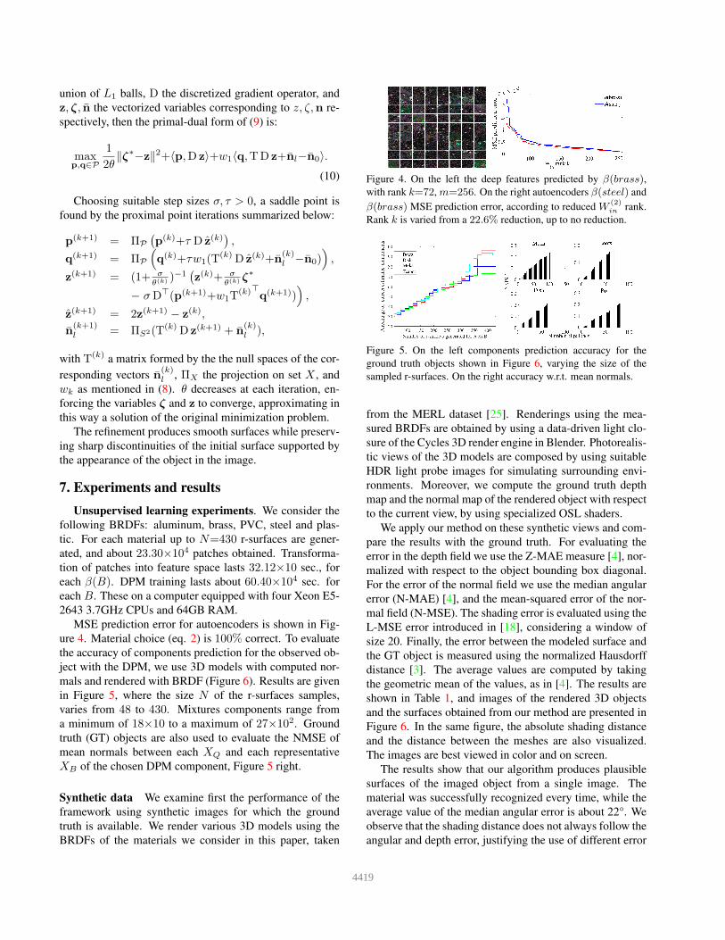
MSE prediction error for autoencoders is shown in Fig-

ure 4. Material choice (eq. 2) is 100% correct. To evaluate

the accuracy of components prediction for the observed ob-

ject with the DPM, we use 3D models with computed nor-

mals and rendered with BRDF (Figure 6). Results are given

in Figure 5, where the size N of the r-surfaces samples,

varies from 48 to 430. Mixtures components range from

a minimum of 18×10 to a maximum of 27×102. Ground

truth (GT) objects are also used to evaluate the NMSE of

mean normals between each XQ and each representative

XB of the chosen DPM component, Figure 5 right.

Synthetic data We examine first the performance of the

framework using synthetic images for which the ground

truth is available. We render various 3D models using the

BRDFs of the materials we consider in this paper, taken

Figure 4. On the left the deep features predicted by β(brass),with rank k=72, m=256. On the right autoencoders β(steel) and

β(brass) MSE prediction error, according to reduced W(2)in

rank.

Rank k is varied from a 22.6% reduction, up to no reduction.

Figure 5. On the left components prediction accuracy for the

ground truth objects shown in Figure 6, varying the size of the

sampled r-surfaces. On the right accuracy w.r.t. mean normals.

from the MERL dataset [25]. Renderings using the mea-

sured BRDFs are obtained by using a data-driven light clo-

sure of the Cycles 3D render engine in Blender. Photorealis-

tic views of the 3D models are composed by using suitable

HDR light probe images for simulating surrounding envi-

ronments. Moreover, we compute the ground truth depth

map and the normal map of the rendered object with respect

to the current view, by using specialized OSL shaders.

We apply our method on these synthetic views and com-

pare the results with the ground truth. For evaluating the

error in the depth field we use the Z-MAE measure [4], nor-

malized with respect to the object bounding box diagonal.

For the error of the normal field we use the median angular

error (N-MAE) [4], and the mean-squared error of the nor-

mal field (N-MSE). The shading error is evaluated using the

L-MSE error introduced in [18], considering a window of

size 20. Finally, the error between the modeled surface and

the GT object is measured using the normalized Hausdorff

distance [3]. The average values are computed by taking

the geometric mean of the values, as in [4]. The results are

shown in Table 1, and images of the rendered 3D objects

and the surfaces obtained from our method are presented in

Figure 6. In the same figure, the absolute shading distance

and the distance between the meshes are also visualized.

The images are best viewed in color and on screen.

The results show that our algorithm produces plausible

surfaces of the imaged object from a single image. The

material was successfully recognized every time, while the

average value of the median angular error is about 22°. We

observe that the shading distance does not always follow the

angular and depth error, justifying the use of different error

4419

0

0.1

0.2

0.3

0.4

0

0.5

1

1.5

2

0

0.1

0.2

0.3

0.4

0.5

0.6

0

0.2

0.4

0.6

0.8

0

0.1

0.2

0.3

0.4

0.5

0.6

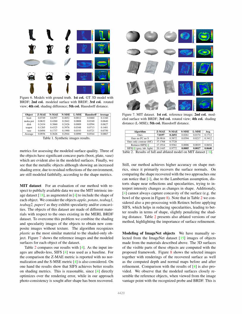
Figure 6. Models with ground truth. 1st col. GT 3D model with

BRDF; 2nd col. modeled surface with BRDF; 3rd col. rotated

view; 4th col. shading difference; 5th col. Hausdorff distance.

Object Z-MAE N-MAE N-MSE L-MSE Hausdorff Average

boot 0.0749 0.6397 0.4052 0.0012 0.0460 0.1160

moka pot 0.0632 0.4260 0.2842 0.0808 0.0340 0.0640

dish 0.2434 0.3060 0.2426 0.0009 0.0594 0.0627

teapot 0.1265 0.4325 0.3976 0.0348 0.0713 0.1401

vase 0.0494 0.1737 0.1990 0.0193 0.0721 0.0750

Average 0.0936 0.3626 0.2944 0.0090 0.0544 0.0867

Table 1. Synthetic images results.

metrics for assessing the modeled surface quality. Three of

the objects have significant concave parts (boot, plate, vase)

which are evident also in the modeled surfaces. Finally, we

see that the metallic objects although showing an increased

shading error, due to residual reflections of the environment,

are still modeled faithfully, according to the shape metrics.

MIT dataset For an evaluation of our method with re-

spect to publicly available data we use the MIT intrinsic im-

age dataset [18], as augmented in [4] to include the shape of

each object. We consider the objects apple, potato, teabag1,

teabag2, paper1 as they exhibit specularity and/or concavi-

ties. The objects of this dataset are made of different mate-

rials with respect to the ones existing in the MERL BRDF

dataset. To overcome this problem we combine the shading

and specularity images of the objects to obtain new com-

posite images without texture. The algorithm recognizes

plastic as the most similar material to the shaded-only ob-

ject. Figure 7 shows the reference images and the modeled

surfaces for each object of the dataset.

Table 2 compares our results with [4]. As the input im-

ages are albedo-less, SIFS [4] was used as a baseline. For

the comparison the Z-MAE metric is reported with no nor-

malization and the S-MSE metric [4] is also considered. On

one hand the results show that SIFS achieves better results

on shading metrics. This is reasonable, since [4] directly

optimizes over the rendering error, while in our approach

photo-consistency is sought after shape has been recovered.

0

0.2

0.4

0.6

0.8

0

0.1

0.2

0.3

0.4

0.5

0.6

0

0.2

0.4

0.6

0.8

0

0.1

0.2

0.3

0.4

0.5

0.6

0.7

0.8

0.9

0

0.2

0.4

0.6

0.8

Figure 7. MIT dataset. 1st col. reference image; 2nd col. mod-

eled surface with BRDF; 3rd col. rotated view; 4th col. shading

distance (L-MSE); 5th col. Hausdorff distance.

Algorithm Z-MAE N-MAE S-MSE L-MSE Avg.

Ours 7.0197 0.2692 0.0261 0.0174 0.1712

Ours no FC no S 26.9816 0.5872 0.0394 0.0217 0.3412

Ours only contour (SfC) 37.1768 0.7728 - - -

Retinex+SIFS[4] 17.1914 0.9361 0.0006 0.0019 0.0654

SIFS[4] (grey, lab. light) 20.1445 0.9772 0.0005 0.0017 0.0640

Table 2. Results of full and ablated model on MIT dataset [18].

Still, our method achieves higher accuracy on shape met-

rics, since it primarily recovers the surface normals. On

comparing the shape recovered with the two approaches one

can notice that [4], due to the Lambertian assumption, dis-

torts shape near reflections and specularities, trying to in-

terpret intensity changes as changes in shape. Additionaly,

[4] cannot always capture concavity of the surface (e.g. the

bowl of the spoon in Figure 8). Note that in Table 2 we con-

sidered also a pre-processing with Retinex before applying

SIFS, which helps in reducing specularities, leading to bet-

ter results in terms of shape, slightly penalizing the shad-

ing distance. Table 2 presents also ablated versions of our

method, highlighting the importance of surface refinement.

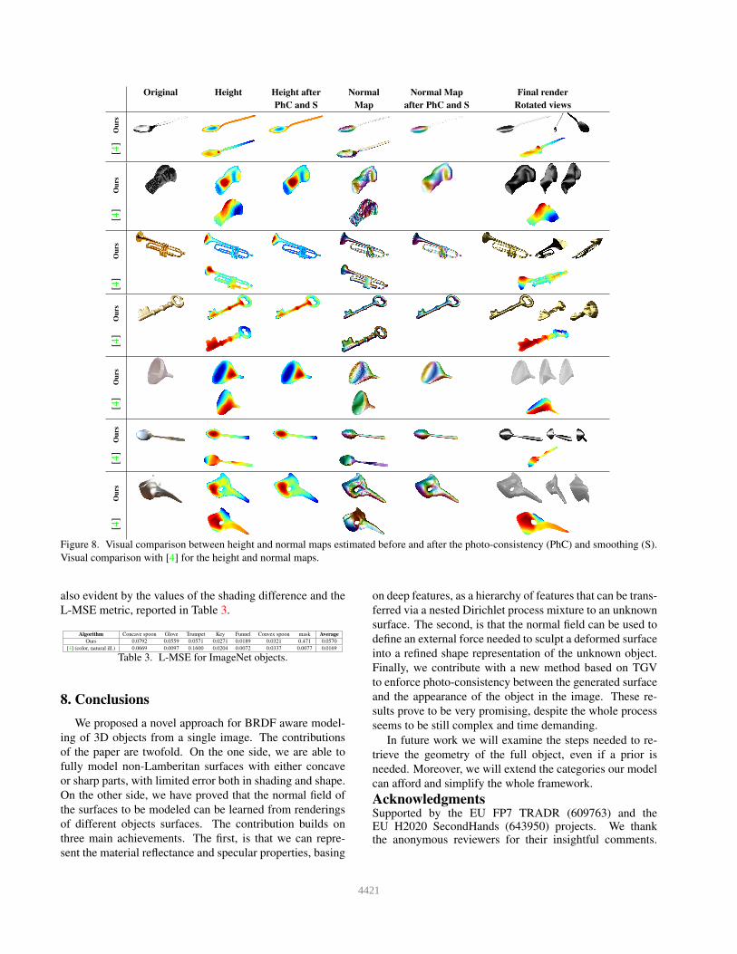
Modeling of ImageNet objects We have manually se-

lected from the ImageNet dataset [15] images of objects

made from the materials described above. The 3D surfaces

of the visible parts of these objects are computed with the

proposed framework. Figure 8 shows the selected images

together with renderings of the recovered surface as well

as the computed depth and normal maps before and after

refinement. Comparison with the results of [4] is also pro-

vided. We observe that the modeled surfaces closely re-

semble the reference objects, when viewed from the image

vantage point with the recognized probe and BRDF. This is

4420

Original Height Height after Normal Normal Map Final render

PhC and S Map after PhC and S Rotated viewsO

urs

[4]

Ou

rs[4

]O

urs

[4]

Ou

rs[4

]O

urs

[4]

Ou

rs[4

]O

urs

[4]

Figure 8. Visual comparison between height and normal maps estimated before and after the photo-consistency (PhC) and smoothing (S).

Visual comparison with [4] for the height and normal maps.

also evident by the values of the shading difference and the

L-MSE metric, reported in Table 3.

Algorithm Concave spoon Glove Trumpet Key Funnel Convex spoon mask Average

Ours 0.0792 0.0559 0.0571 0.0271 0.0189 0.0321 0.471 0.0570

[4] (color, natural ill.) 0.0669 0.0097 0.1600 0.0204 0.0072 0.0337 0.0077 0.0169

Table 3. L-MSE for ImageNet objects.

8. Conclusions

We proposed a novel approach for BRDF aware model-

ing of 3D objects from a single image. The contributions

of the paper are twofold. On the one side, we are able to

fully model non-Lamberitan surfaces with either concave

or sharp parts, with limited error both in shading and shape.

On the other side, we have proved that the normal field of

the surfaces to be modeled can be learned from renderings

of different objects surfaces. The contribution builds on

three main achievements. The first, is that we can repre-

sent the material reflectance and specular properties, basing

on deep features, as a hierarchy of features that can be trans-

ferred via a nested Dirichlet process mixture to an unknown

surface. The second, is that the normal field can be used to

define an external force needed to sculpt a deformed surface

into a refined shape representation of the unknown object.

Finally, we contribute with a new method based on TGV

to enforce photo-consistency between the generated surface

and the appearance of the object in the image. These re-

sults prove to be very promising, despite the whole process

seems to be still complex and time demanding.

In future work we will examine the steps needed to re-

trieve the geometry of the full object, even if a prior is

needed. Moreover, we will extend the categories our model

can afford and simplify the whole framework.

AcknowledgmentsSupported by the EU FP7 TRADR (609763) and theEU H2020 SecondHands (643950) projects. We thankthe anonymous reviewers for their insightful comments.

4421

References

[1] G. Andrew and J. Gao. Scalable training of l1-regularized

log-linear models. In ICML, pages 33–40, 2007. 4

[2] C. E. Antoniak. Mixtures of dirichlet processes with applica-

tions to bayesian nonparametric problems. Ann. Stat., pages

1152–1174, 1974. 4

[3] N. Aspert, D. Santa Cruz, and T. Ebrahimi. Mesh: measur-

ing errors between surfaces using the hausdorff distance. In

ICME (1), pages 705–708, 2002. 6

[4] J. Barron and J. Malik. Shape, illumination, and reflectance

from shading. TPAMI, 2015. 1, 6, 7, 8

[5] H. Barrow and J. Tenenbaum. Recovering intrinsic scene

characteristics from images. Computer Vision Syst., 1978. 2

[6] Y. Bengio, A. Courville, and P. Vincent. Representa-

tion learning: A review and new perspectives. TPAMI,

35(8):1798–1828, 2013. 4

[7] D. M. Blei, T. L. Griffiths, and M. I. Jordan. The nested

chinese restaurant process and bayesian nonparametric in-

ference of topic hierarchies. Journal of the ACM (JACM),

57(2):7, 2010. 1, 3

[8] D. M. Blei and M. I. Jordan. Variational inference for dirich-

let process mixtures. Bayes. Anal., 1(1):121–143, 2006. 4

[9] K. Bredies, K. Kunisch, and T. Pock. Total generalized vari-

ation. SIAM JIS, 3(3):492–526, 2010. 5

[10] M. Burger and S. Osher. A guide to the tv zoo. In Level Set

and PDE Based Reconstruction Methods in Imaging, pages

1–70. Springer, 2013. 5

[11] A. Chambolle and T. Pock. A First-Order Primal-Dual Al-

gorithm for Convex Problems with Applications to Imaging.

JMIV, 40(1):120–145, 2010. 5

[12] M. K. Chandraker, C. F. Kahl, and D. J. Kriegman. Reflec-

tions on the generalized bas-relief ambiguity. In CVPR, vol-

ume 1, pages 788–795, 2005. 2

[13] I. Csiszar. Maxent, mathematics, and information theory. In

Max. entropy and Bayesian methods, pages 35–50. Springer

Science & Business Media, 1996. 4

[14] P. Debevec. Rendering synthetic objects into real scenes:

Bridging traditional and image-based graphics with global

illumination and high dynamic range photography. In ACM

SIGGRAPH, page 32. ACM, 2008. 3

[15] J. Deng, W. Dong, R. Socher, L.-J. Li, K. Li, and L. Fei-Fei.

ImageNet: A Large-Scale Hierarchical Image Database. In

CVPR, 2009. 1, 3, 7

[16] T. S. Ferguson. A bayesian analysis of some nonparametric

problems. Ann. Stat., pages 209–230, 1973. 1, 4

[17] J. Filip and R. Vavra. Template-based sampling of

anisotropic BRDFs. Comp. Graph. Forum, 2014. 2

[18] R. Grosse, M. Johnson, E. H. Adelson, and W. Freeman.

Ground truth dataset and baseline evaluations for intrinsic

image algorithms. In ICCV, pages 2335–2342, 2009. 6, 7

[19] G. E. Hinton and R. R. Salakhutdinov. Reducing the

dimensionality of data with neural networks. Science,

313(5786):504–507, 2006. 4

[20] B. K. Horn. Understanding image intensities. Artificial in-

telligence, 8(2):201–231, 1977. 1

[21] S. Jain and R. M. Neal. A split-merge markov chain monte

carlo procedure for the dirichlet process mixture model.

Journal of Computational and Graphical Statistics, 2012. 4

[22] E. H. Land and J. McCann. Lightness and Retinex theory.

JOSA, 61(1):1–11, 1971. 2, 5

[23] S. Magda, D. J. Kriegman, T. Zickler, and P. N. Belhumeur.

Beyond Lambert: Reconstructing surfaces with arbitrary

BRDFs. In ICCV, pages 391–398, 2001. 1, 2

[24] S. P. Mallick, T. E. Zickler, D. J. Kriegman, and P. N. Bel-

humeur. Beyond Lambert: Reconstructing specular surfaces

using color. In CVPR, pages 619–626, 2005. 1

[25] W. Matusik, H. Pfister, M. Brand, and L. McMillan. A data-

driven reflectance model. In ACM SIGGRAPH, pages 759–

769, 2003. 1, 2, 6

[26] P. Munro and D. Zipser. Image compression by back propa-

gation: an example of extensional programming. Models of

cognition: rev. of cognitive science, 1:208, 1989. 1, 4

[27] T. Narihira, M. Maire, and S. X. Yu. Direct intrinsics: Learn-

ing albedo-shading decomposition by convolutional regres-

sion. In ICCV, 2015. 2

[28] F. Natola, V. Ntouskos, M. Sanzari, and F. Pirri. Bayesian

non-parametric inference for manifold based mocap repre-

sentation. In ICCV, pages 4606–4614, 2015. 4

[29] S. Nayar, K. Ikeuchi, and T. Kanade. Surface reflection:

physical and geometrical perspectives. TPAMI, 13(7):611–

634, 1991. 2

[30] J. Ngiam, A. Coates, A. Lahiri, B. Prochnow, Q. V. Le, and

A. Y. Ng. On optimization methods for deep learning. In

ICML, pages 265–272, 2011. 4

[31] F. E. Nicodemus. Directional reflectance and emissivity of

an opaque surface. Applied optics, 4(7):767–775, 1965. 1, 2

[32] V. Ntouskos, M. Sanzari, B. Cafaro, F. Nardi, F. Natola,

F. Pirri, and M. Ruiz. Component-wise modeling of artic-

ulated objects. In ICCV, pages 2327–2335, 2015. 4

[33] B. A. Olshausen and D. J. Field. Sparse coding with an over-

complete basis set: A strategy employed by v1? Vision re-

search, 37(23):3311–3325, 1997. 1, 4

[34] G. Oxholm and K. Nishino. Shape and reflectance from nat-

ural illumination. In ECCV, pages 528–541. Springer, 2012.

1, 2

[35] J. Paisley, C. Wang, D. M. Blei, and M. I. Jordan. Nested hi-

erarchical dirichlet processes. Pattern Analysis and Machine

Intelligence, IEEE Transactions on, 37(2):256–270, 2015. 3

[36] T. Papadhimitri and P. Favaro. A new perspective on un-

calibrated photometric stereo. In CVPR, pages 1474–1481,

2013. 5

[37] D. Reddy, A. Agrawal, and R. Chellappa. Enforcing integra-

bility by error correction using l1-minimization. In CVPR,

pages 2350–2357, 2009. 5

[38] S. R. Richter and S. Roth. Discriminative shape from shading

in uncalibrated illumination. In CVPR, pages 1128–1136,

2015. 2

[39] A. Rodriguez, D. B. Dunson, and A. E. Gelfand. The nested

dirichlet process. Journal of the American Statistical Asso-

ciation, 2008. 3

[40] F. Romeiro and T. Zickler. Inferring reflectance under real-

world illumination. Tech. report, Cambridge, MA, 2010. 2

4422

[41] A. Saxena, M. Sun, and A. Y. Ng. Make3d: Learning 3d

scene structure from a single still image. TPAMI, 31(5):824–

840, 2009. 2

[42] M. Schmidt, D. Kim, and S. Sra. Projected newton-type

methods in machine learning. Optimization for Machine

Learning, page 305, 2012. 4

[43] G. Strang and G. J. Fix. An analysis of the finite element

method, volume 212. Prentice-Hall, 1973. 1, 4, 5

[44] E. B. Sudderth. Graphical models for visual object recogni-

tion and tracking. PhD thesis, MIT, 2006. 4

[45] D. Terzopoulos, J. Platt, A. Barr, and K. Fleischer. Elastically

deformable models. In ACM SIGGRAPH, pages 205–214,

1987. 2, 4

[46] Y. Vasilyev, Y. Adato, T. Zickler, and O. Ben-Shahar. Dense

specular shape from multiple specular flows. In CVPR, pages

1–8, 2008. 2

[47] L. A. Vese and T. F. Chan. A multiphase level set framework

for image segmentation using the mumford and shah model.

IJCV, 50(3):271–293, 2002. 1, 3

[48] Y. Xiong, A. Chakrabarti, R. Basri, S. J. Gortler, D. W. Ja-

cobs, and T. Zickler. From shading to local shape. TPAMI,

37(1):67–79, 2015. 2

[49] B. Zeisl, C. Zach, and M. Pollefeys. Variational regulariza-

tion and fusion of surface normal maps. In 3DV, volume 1,

pages 601–608, 2014. 5

[50] R. Zhang, P.-S. Tsai, J. Cryer, and M. Shah. Shape-from-

shading: a survey. TPAMI, 21(8):690–706, Aug 1999. 2

4423