single image blind deconvolution with higher-order texture ... · single image blind deconvolution...

Single Image Blind Deconvolution withHigher-Order Texture Statistics ?

Manuel Martinello and Paolo Favaro

Heriot-Watt UniversitySchool of EPS, Edinburgh EH14 4AS, UK

Abstract. We present a novel method for solving blind deconvolution,i.e., the task of recovering a sharp image given a blurry one. We focus onblurry images obtained from a coded aperture camera, where both thecamera and the scene are static, and allow blur to vary across the imagedomain. As most methods for blind deconvolution, we solve the prob-lem in two steps: First, we estimate the coded blur scale at each pixel;second, we deconvolve the blurry image given the estimated blur. Ourapproach is to use linear high-order priors for texture and second-orderpriors for the blur scale map, i.e., constraints involving two pixels at atime. We show that by incorporating the texture priors in a least-squaresenergy minimization we can transform the initial blind deconvolutiontask in a simpler optimization problem. One of the striking features ofthe simplified optimization problem is that the parameters that definethe functional can be learned offline directly from natural images via sin-gular value decomposition. We also show a geometrical interpretation ofimage blurring and explain our method from this viewpoint. In doing sowe devise a novel technique to design optimally coded apertures. Finally,our coded blur identification results in computing convolutions, ratherthan deconvolutions, which are stable operations. We will demonstratein several experiments that this additional stability allows the method todeal with large blur. We also compare our method to existing algorithmsin the literature and show that we achieve state-of-the-art performancewith both synthetic and real data.

Keywords: coded aperture, single image, image deblurring, depth esti-mation.

1 Introduction

Recently there has been enormous progress in image deblurring from a singleimage. Perhaps one of the most remarkable results is to have shown that itis possible to extend the depth of field of a camera by modifying the cameraoptical response [1–7]. Moreover, techniques based on applying a mask at thelens aperture have demonstrated the ability to recover a coarse depth of the

? This research was partly supported by SELEX Galileo grant SELEX/HWU/2010/SOW3.

2 Manuel Martinello, Paolo Favaro

(a) (b)

Fig. 1. Results on an outdoor scene [exposure time 1/200s]. (a) Blurry codedimage captured with mask b (see Fig. 4). (b) Sharp image reconstructed with ourmethod.

scene [4, 5, 8]. Depth has then been used for digital refocusing [9] and advancedimage editing.

In this paper we present a novel method for image deblurring and demon-strate it on blurred images obtained from a coded aperture camera. Our algo-rithm uses as input a single blurred image (see Fig. 1 (a)) and automaticallyreturns the corresponding sharp one (see Fig. 1 (b)). Our main contribution is toprovide a computationally efficient method that achieves state-of-the-art perfor-mance in terms of depth and image reconstruction with coded aperture cameras.We demonstrate experimentally that our algorithm can deal with larger amountsof blur than previous coded aperture methods.

One of the leading approaches in the literature [5] recovers a sharp image bysequentially testing a deconvolution method for several given hypotheses for theblur scale. Then, the blur scale that yields a sharp image that is consistent withboth the model and the texture priors is chosen. In contrast, in our approach weshow that one can identify the blur scale by computing convolutions, rather thandeconvolutions, of the blurry image with a finite set of filters. As a consequence,our method is numerically stable especially when dealing with large blur scales.In the next sections, we present all the steps needed to define our algorithm forimage deblurring. The task is split in two steps: First the blur scale is identifiedand second, the coded image is deblurred with the estimated blur scale. Wepresent an algorithm for blur scale identification in section 3.1. Image deblurringis then solved iteratively in section 3.2. A discussion on mask selection is thenpresented in section 4.1. Comparisons to existing methods are shown in section 5.

1.1 Prior Work

This work relates to several fields ranging from computer vision to image andsignal processing, and from optics to astronomy and computer graphics. Forsimplicity, we group past work based on the technique being employed.

Single Image Blind Deconvolution with Higher-Order Texture Statistics 3

Coded Imaging: Early work in coded imaging appears in the field of as-tronomy. One of the most interesting pattern designs is the Modified UniformlyRedundant Arrays (MURA) [10] for which a simple coding and decoding pro-cedure was devised (see one such pattern in Fig. 4). In our tests the MURApattern seems very well behaved, but too sensitive to noise (see Fig. 5). Codedpatterns have also been used to design lensless systems, but these systems re-quire either long exposures or are sensitive to noise [11]. More recently, codingof the exposure [12] or of the aperture [4] has been used to preserve high spatialfrequencies in blurred images so that deblurring is well-posed. We test the maskproposed in [4] and find that it works well for image deblurring, but not for blurscale identification. A mask that we have tested and has yielded good perfor-mance is the four-holes mask of Hiura and Matsuyama [13]. In [13] however, theauthors used multiple images. A study on good apertures for deblurring multiplecoded images via Wiener filtering has instead led to two novel designs [14, 15].Although the masks were designed to be used together, we have tested each ofthem independently for comparisons purposes. We found, as predicted by theauthors, that the masks are quite robust to noise and quite well designed forimage deblurring. Image deblurring and depth estimation with a coded aper-ture camera has also been demonstrated by Levin et al. [5]. One of their maincontributions is the design of an optimal mask. We indeed find this mask quiteeffective both on synthetic data and real data. However, as already noticed in[16], we have found that the coded aperture technique, if approached as in [5],fails when dealing with large blur amounts. The method we propose in this pa-per, instead, overtakes this limitation, especially when using the four-hole mask.Finally, a design based on annular masks has also been proposed in [17] andhas been exploited for depth estimation in [3]. We also tested this mask in ourexperiments, but, contrary to our expectations, we did not find its performancesuperior to the other masks.

3D Point Spread Functions: While there are several techniques to ex-tract depth from images, we briefly mention some recent work by Greengard etal. [18] because their optical design included and exploited diffraction effects.They investigated 3D point spread functions (PSF) whose transverse cross sec-tions rotate as a result of diffraction, and showed that such PSFs yield an orderof magnitude increase in the sensitivity with respect to depth variations. Themain drawback however, is that the depth range and resolution is limited dueto the angular resolution of the reconstructed PSF.

Depth-Invariant Blur: An alternative approach to coded imaging is wave-front coding. The key idea is to use aspheric lenses to render the lens pointspread function (PSF) depth-invariant. Then, shift-invariant deblurring with afixed known blur can be applied to sharpen the image [19, 20]. However, whilethe results are quite promising, the PSF is not fully depth-invariant and artifactsare still present in the reconstructed image. Other techniques based on depth-invariant PSFs exploit the chromatic aberrations of lenses [7] or use diffusion[21]. However, in the first case, as the focal sweep is across the spectrum, themethod is mostly designed for grayscale imaging. While the results shown in


these recent works are stunning, there are two inherent limitations: 1) Depth islost in the imaging process; 2) In general, as method based on focal sweep arenot exactly depth-invariant, the deblurring performance decays for objects thatare too close or too far away from the camera.

Multiple viewpoint: The extension of the depth of field can also be achievedby using multiple images and/or multiple viewpoints. One technique is to ob-tain multiple viewpoints by capturing multiple coded images [8, 13, 22] or bycapturing a single image by using a plenoptic camera [9, 6, 23, 24]. These meth-ods however, exploit multiple images or require a more costly optical design (e.g.,a calibrated microlens array).

Motion Deblurring and Blind Deconvolution: This work also relatesto work in blind deconvolution, and in particular on motion deblurring. Therehas been a quite steady progress in uniform motion deblurring [25–29] thanksto the modeling and exploitation of texture statistics. Although these methodsdeal with an unknown and general blur pattern, they assume that blur is notchanging across the image domain. More recently, the space-varying case hasbeen studied [30–32] albeit with some restrictions on the type of motion or thescene depth structure.

Blurred face recognition: Work in the recognition of blurred faces [33]is also related to our method. Their approach extracts features from motion-blurred images of faces and then uses the subspace distance to identify the blur.In contrast, our method can be applied to space-varying blur and our analysisprovides a novel method to evaluate (and design) masks.

2 Single Image Blind Deconvolution

Blind deconvolution from a single image is a very challenging problem: We needto recover more unknowns than the available observations. This challenge willbe illustrated in the next section, where we present the image formation modelof a blurred image obtained from a coded aperture camera. To make the prob-lem feasible and well-behaved, one can introduce additional constraints on thesolution. In particular, we constrain the higher-order statistics of sharp texture(sec. 2.2) and impose that the blur scale be piecewise smooth across the imagepixels (sec. 2.3).

2.1 Image Model

In the simplest instance, a blurred image of a plane facing the camera can bedescribed via the convolution of a sharp image with the blur kernel. However, theconvolutional model breaks down with more general surfaces and, in particular,at occlusion boundaries. In this case, one can describe a blurred image with alinear model. For the sake of notational simplicity, we write images as columnvectors, where all pixels are sorted in lexicographical order. Thus, a blurredimage with N pixels is a column vector g ∈ RN . Similarly, a sharp image with


M pixels is a column vector f ∈ RM . Then, g satisfies

g = Hdf , (1)

where the N ×M matrix Hd represents the coded blur. d is a column vectorwith M pixels and collects the blur scale corresponding to each pixel of f . Thei-th column of Hd is an image, rearranged as a vector, of the coded blur withscale di generated by the i-th pixel of f . Notice that this model is indeed ageneralization of the convolutional case. In the convolutional model, Hd reducesto a Toeplitz matrix.

Our task is to recover the unknown sharp image f given the blurred image g.To achieve this goal it is necessary to recover the blur scale at each pixel d. Thetheory of linear algebra tells us that: If N = M and the equations in eq. (1) arenot linearly dependent, and we are given both g and Hd, then we can recoverthe sharp image f . However, in our case we are not given the matrix Hd andthe blurred image g is affected by noise. This introduces two challenges: First,to obtain Hd we need to retrieve the blur scale d; second, because of noise ing and of the ill-conditioning of the linear system in eq. (1), the estimation off might be unstable. The first challenge implies that we do not have a uniquesolution. The second challenge implies that even if the solution were unique, itsestimation would not be reliable. However, not all is lost. It is possible to addmore equations to eq. (1) until a unique reliable solution can be obtained. Thistechnique is based on observing that, typically, one expects the unknown sharpimage and blur scale map to have some regularity. For instance, both sharptextures and blur scale maps are not likely to look like noise. In the next twosections we will present and illustrate our sharp image and blur scale priors.

2.2 Sharp Image Prior

Images of the real world exhibit statistical regularities that have been studiedintensively in the past 20 years and have been linked to the human visual systemand its evolution [34]. For the purpose of image deblurring, the most importantaspect of this study is that natural images form a much smaller subset of allpossible images. In general, the characterization of the statistical properties ofnatural images is done by applying a given transform, typically related to acomponent of human vision. Among the most common statistics used in imageprocessing are the second order statistics, i.e., relations between pairs of pixels.For instance, this category includes the distributions of image gradients [35, 36].

However, a more accurate account of the image structure can be capturedwith high-order statistics, i.e., relations between several pixels. In this work, weconsider this general case, but restrict the relations to linear ones of the form

Σf ' 0 (2)

where Σ is a rectangular matrix. Eq. (2) implies that all sharp images liveapproximately on a subspace. Despite their crude simplicity, these linear con-straints allow for some flexibility. For example, the case of second-order statistics


results in rows of Σ with only two nonzero values. Also, by designing Σ one canselectively apply the constraints only on some of the pixels. Another example isto choose each row of Σ as a Haar feature applied to some pixels. Notice thatin our approach we do not make any of these choices. Rather, we estimate Σdirectly from natural images.

Natural image statistics, such as gradients, typically exhibit a peaked dis-tribution. However, performing inference on such distributions results in mini-mizations of non convex functionals for which we do not have probably optimalalgorithms. Furthermore, we are interested in simplifying the optimization taskas much as possible to gain in computational efficiency. This has led us to enforcethe linear relation above by minimizing the convex cost

‖Σf‖22. (3)

As we do not have an analytical expression for Σ that satisfies eq. (2), we needto learn it directly from the data. We will see later that this step is necessaryonly when performing the deconvolution step given the estimated blur. Instead,when estimating the blur scale our method allows us to use Σ implicitly, i.e.,without ever recovering it.

2.3 Blur Scale Prior

The statistics of range images can be characterized with an approach similarto that for optical images [37]. The study in [37] verified the random collagemodel, i.e., that a scene is a collection of piecewise constant surfaces. This hasbeen observed in the distributions of Haar filter responses on the logarithmof the range data, which showed strong cusps in the isoprobability contours.Unfortunately, a prior following these distributions faithfully would result in nonconvex energy minimization. A practical convex solution to enforce the piecewiseconstant model, is to use total variation [38]. Common choices are the isotropicand anisotropic total variation. In our algorithm we have implemented the latter.We minimize ‖∇d‖1, i.e., the sum of the absolute value of the components ofthe gradient of d.

3 Blur Scale Identification and Image Deblurring

We can combine the image model introduced in sec. 2.1 with the priors in sec. 2.2and 2.3 and formulate the following energy minimization problem:

d, f = argmind,f

‖g −Hdf‖22 + α‖Σf‖22 + β‖∇d‖1, (4)

where the parameters α, β > 0 determine the amount of regularization for tex-ture and blur scale respectively. Notice that the formulation above is commonto many approaches including, in particular, [5]. Our approach, however, in ad-dition to using a more accurate blur matrix Hd, considers different priors anda different depth identification procedure.


Our next step is to notice that, given d, the proposed cost is simply a least-squares problem in the unknown sharp texture f . Hence, it is possible to computef in closed-form and plug it back in the cost functional. The result is a muchsimpler problem to solve. We summarize all the steps in the following Theorem:

Theorem 1. The set of extrema of the minimization (4) coincides with the setof extrema of the minimization

d = argmin

d‖H⊥d g‖22 + β‖∇d‖1

f =(αΣTΣ +HT

dHd

)−1

HTdg

(5)

where H⊥d.= I −Hd

(αΣTΣ +HT

dHd

)−1HT

d , and I is the identity matrix.

Proof. See Appendix.

Notice that the new formulation requires the definition of a square and symmetricmatrix H⊥d . This matrix depends on the parameter α and the prior matrix Σ,both of which are unknown. However, for the purpose of estimating the unknownblur scale map d, it is possible to bypass the estimation of α and Σ by learningdirectly the matrix H⊥d from data.

3.1 Learning Procedure and Blur Scale Identification

We break down the complexity of solving eq. (5) by using local blur uniformity,i.e., by assuming that blur is constant within a small region of pixels. Then,we further simplify the problem by considering only a finite set of L blur sizesd1, . . . , dL. In practice, we find that both assumptions work well. The local bluruniformity holds reasonably well except at occluding boundaries, which form asmall subset of the image domain. At occluding boundaries the solution tends tofavor small blur estimates. We also found experimentally that the discretizationis not a limiting factor in our method. The number of blur sizes L can be setto a value that matches the level of accuracy of the method without reaching aprohibitive computational load.

Now, by combining the assumptions we find that eq. (5) at one pixel x

d(x) = argmind(x)

‖H⊥d (x)g‖22 + β‖∇d(x)‖1 (6)

can be approximated by

d(x) = argmind(x)

‖H⊥d(x)gx‖22 (7)

where gx is a column vector of δ2 pixels extracted from a δ × δ patch centeredat the pixel x of g. Experimentally, we find that the size δ of the patch shouldnot be smaller than the maximum scale of the coded blur in the captured imageg. H⊥d(x) is a δ2 × δ2 matrix that depends on the blur size d(x) ∈ {d1, . . . , dL}.


So we assume that H⊥d (x,y) ' 0 for y such that ‖y − x‖1 > δ/2. Notice thatthe term β‖∇d‖1 drops because of the local blur uniformity assumption.

The next step is to explicitly compute H⊥d(x). Since the blur size d(x) isone of L values, we only need to compute H⊥d1 , . . . ,H

⊥dL

matrices. As each H⊥di

depends on α and the local Σ, we propose to learn each H⊥didirectly from data.

Suppose that we are given a set of T column vectors gx1 , . . . , gxTextracted from

blurry images of a plane parallel to the camera image plane. The column vectorswill all share the same blur scale di. Hence, we can rewrite the cost functionalin eq. (7) for all x as

‖H⊥diGi‖22 (8)

where Gi.= [gx1 · · · gxT

]. By definition of Gi, ‖H⊥diGi‖22 = 0. Hence, we find

thatH⊥dican be computed via the singular value decomposition ofGi = UiSiV

Ti .

If Ui = [Udi Qdi ] where Qdi corresponds to the singular values of Si that arezero (or negligible), then H⊥di

= QdiQTdi

. The procedure is then repeated foreach blur scale di with i = 1, . . . , L.

Next, we can use the estimated matrices H⊥d1 , . . . ,H⊥dL

on a new image gand optimize with respect to d:

d = argmind

∑

x

‖H⊥d(x)gx‖22 + β‖∇d(x)‖1. (9)

The first term represents unitary terms, i.e., terms that are defined on singlepixels; the second term represents binary terms, i.e., terms that are defined onpairs of pixels. The minimization problem (9) can then be solved efficiently viagraph cuts [39].

Notice that the procedure above can be applied to other surfaces as well, sothat instead of a collection of parallel planes, one can consider, for example, acollection of quadratic surfaces. Also, notice that there are no restrictions on thesize of a patch. In particular, the same procedure can be applied to a patch ofthe size of the input image. In our experiments for depth estimation, however,we consider only small patches and parallel planes as local surfaces.

3.2 Image Deblurring

In the previous section we have devised a procedure to compute the blur scaleat each pixel d. In this section we assume that d is given and devise a procedureto compute the image f . In principle, one could use the closed-form solution

f =(αΣTΣ +HT

dHd

)−1

HTdg. (10)

However, notice that computing this equation entails solving a large matrixinversion, which is not practical for moderate image dimensions. A simpler ap-proach is to solve the least squares problem (4) in f via an iterative method.Therefore, we consider solving the problem

f = argminf‖g −Hdf‖22 + α‖Σf‖22 (11)


by using a least-squares conjugate gradient descent algorithm in f [40]. Themain component for the iteration in f is the gradient ∇Ef of the cost (11) withrespect to f

∇Ef =(αΣTΣ +HT

dHd

)f −HT

dg. (12)

The descent algorithm iterates until ∇Ef ' 0. Because of the convexity of thecost functional with respect to f , the solution is also a global minimum.

To compute Σ we use a database of sharp images F = [f1 · · ·fT ] where{fi}i=1,...,T are sharp images rearranged as column vectors, and compute the sin-gular value decomposition F = UFΣFV

TF . Then, we partition UF = [UF,1 UF,2]

such that UF,2 corresponds to the smallest singular values of ΣF . The high-orderprior is defined as Σ .= UF,2U

TF,2, such that we have Σfi ≈ 0. The regularization

parameter α is instead manually tuned. The matrixHd is computed as describedin Section 2.1.

4 A Geometric Viewpoint on Blur Scale Identification

In the previous sections we have seen that the blur scale at each pixel can beobtained by minimizing eq. (9). We search among matrices H⊥d1 , . . . ,H

⊥dL

theone that yields the minimum `2 norm when applied to the vector gx. We showthat this has a geometrical interpretation: Each matrix H⊥di

defines a subspaceand ‖H⊥di

gx‖22 is the distance of each vector gx from that subspace.Recall that H⊥di

= QdiQT

diand that Ui = [Udi

Qdi] is an orthonormal

matrix. Then, we obtain that ‖H⊥digx‖22 = ‖QdiQ

Tdigx‖22 = ‖QT

digx‖22 = ‖gx‖22−

‖UTdigx‖22. If we now divide by the scalar number ‖gx‖22, we obtain exactly the

square of the subspace distance [41]

M(g,Udi) =

√√√√1−K∑

j=1

(UTdi,j

g

‖g‖

)2

(13)

where K is the rank of the subspace Udi, Udi

= [Udi,1 . . . Udi,K ], and Udi,j ,j = 1, · · · ,K are orthonormal vectors.

The geometrical interpretation brings a fresh look to image blurring anddeblurring. Consider the image model (1). Let us take the singular value decom-position of the blur matrix Hd

Hd = UdSdVTd (14)

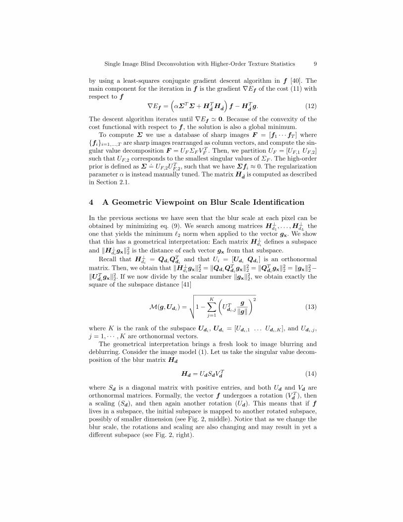
where Sd is a diagonal matrix with positive entries, and both Ud and Vd areorthonormal matrices. Formally, the vector f undergoes a rotation (V Td ), thena scaling (Sd), and then again another rotation (Ud). This means that if flives in a subspace, the initial subspace is mapped to another rotated subspace,possibly of smaller dimension (see Fig. 2, middle). Notice that as we change theblur scale, the rotations and scaling are also changing and may result in yet adifferent subspace (see Fig. 2, right).


f1

f2

f3

(a)

g1

g2g3

Hd1

(b)

g1

g2

g3

Hd2

(c)

Fig. 2. Coded images subspaces. (a) Image patches on a subspace. (b) Subspacecontaining images blurred with Hd1 ; blurring has the effect of rotating and possiblyreducing the dimensionality of the original subspace. (c) Subspace containing imagesblurred with Hd2 .

It is important to understand that rotations of the vector f can result inblurring. To clarify this, consider blurred and sharp images with only 3 pixels(we cannot visualize the case of more than 3 pixels), i.e., g1 = [g1,x g1,y g1,z]T

and f1 = [f1,x f1,y f1,z]T . Then, we can plot the vectors g1 and f1 as 3D points(see Fig. 2). Let ‖g1‖ = 1 and ‖f1‖ = 1. Then, we can rotate f1 about the originand overlap it exactly on g1. In this case rotation corresponded to blurring. Theopposite is also true. We can rotate the vector g1 onto the vector f1 and thusperform deblurring. Furthermore, notice that in this simple example the mostblurred images are vectors with identical entries. Such blurred images lie alongthe diagonal direction [1 1 1]T . In general, blurry images tend to have entrieswith similar values and hence tend to cluster around the diagonal direction.

Our ability to discriminate between different blur scales in a blurry imageboils down to being able to determine the subspaces where the patches of suchblurry image live. If sharp images do not live on a subspace, but uniformly inthe entire space, our only way to distinguish the blur size is that the blurringHd scales some dimensions of f to zero and that the scaling varies with blursize. This case has links to the zero-sheet approach in the Fourier domain [42].However, if the sharp images live on a subspace, the blurring Hd may preserve


Input: A single coded image g and a collection of coded images of L planarscenes.

Output: The blur scale map d of the scene.Preprocessing (offline)Pick an image patch size larger than twice the maximum blur scale;for i = 1, . . . , L do

Compute the singular value decomposition UiSiVTi of a collection of image

patches coded with blur scale di ;Calculate the subspace Udi as the columns of Ui corresponding to nonzerosingular values of Si;

endBlur identification (online)

Solve d = arg mind∈{d1,··· ,dL}P

xM2(gx,Ud) + β

‖gx‖22‖∇d(x)‖1.

Algorithm 1: Blur scale identification from a single coded image via thesubspace distance method.

all the directions and blur scale identification is still possible by determining therotation of the sharp images subspace. This is the principle that we exploit.

Notice that the evaluation of the subspace distance M involves the calcu-lation of the inner product between a patch and a column of Udi

. Hence, thiscalculation can be done exactly as the convolution of a column ofUdi

, rearrangedas an image patch, with the whole image g. We can conclude that the algorithmrequires computing a set of L×K convolutions with the coded image, which isa stable operation of polynomial computational complexity. As we have shownthat minimizing eq. (13) is equivalent to minimizing ‖H⊥di

gx‖22 up to a scalarvalue, we summarize the blur scale identification procedure in Algorithm 1.

4.1 Coded Aperture Selection

In this section we discuss how to obtain an optimal pattern for the purpose ofimage deblurring. As pointed out in [19] we identify two main challenges: Thefirst one is that accurate deblurring requires accurate identification of the blurscale; the second one is that accurate deblurring requires little texture loss dueto blurring. A first step towards addressing these challenges is to define a metricfor blur scale identification and a metric for texture loss. Our metric for blurscale identification can be defined directly from section 4. Indeed, the ability todetermine which subspace a coded image patch belongs to can be measured viathe distance between the subspaces associated to each blur scale

M(Ud1 ,Ud2) =√K −

∑

i,j

(UTd1,i

Ud2,j

)2

. (15)

Clearly, the wider apart all the subspaces are, and the less prone to noise thesubspace association is. We find that a good visual summary of the “spacing”


d

d

(Ud10, Ud20) = !K

(Ud25, Ud25) = 0

8 Manuel Martinello and Paolo Favaro



Compute the singular value decomposition UiSiVT

i of a collection of imagespatches coded with blur scale di ;Calculate the subspace Udi as the columns of Ui corresponding to nonzerosingular values of Si;


for each patch gx centered at a pixel x of g do

Solve d(x) = arg mind∈{d1,··· ,dL} M(gx , Ud).end


the distance between the subspaces associated to each blur scale211 211

M(Ud1 ,Ud2) =�

K −�

i,j

�UT

d1,iUd2,j

�2

. (14)

Clearly, the wider apart all the subspaces are, and the less prone to noise the212 212

subspace association is. We find that a good visual summary of the “spacing”213 213

between all the subspaces is a (symmetric) matrix with distances between any214 214

two subspaces. We compute such matrix for a conventional camera and the215 215

coded apertures in Fig. 4 and show the result in Fig. 3. In each distance matrix,216 216

subspaces associated to blur scales ranging from the smallest to the largest ones217 217

are arranged along the rows from left to right and along the columns from top to218 218

bottom. Along the diagonal the distance is necessarily 0 as we compare identical219 219

subspaces. Notice, also, that by definition the metric cannot exceed√

K, where220 220

K is the maximum rank among the subspaces. The rank K can be used to address221 221

the second challenge, i.e., the definition of a metric for texture loss. So far we have222 222

seen that blurring can be interpreted as a combination of rotations and scaling.223 223

Deblurring can then be interpreted as a combination of rotations and scaling in224 224

the opposite direction. However, when blurring scales some directions to 0, part225 225

of the texture content has been lost. This suggests that a simple measure for226 226

texture loss is the dimension of the coded subspace: The higher the dimension227 227

and the more texture content we can restore. As the (coded images) subspace228 228

dimension is K, we can immediately conclude that the subspace distance matrix229 229

that most closely resembles the ideal distance matrix (see Fig. 2, top-left) is230 230

the one that simultaneously achieves the best depth identification and the least231 231

8 Manuel Martinello and Paolo Favaro



Compute the singular value decomposition UiSiVT

i of a collection of imagespatches coded with blur scale di ;Calculate the subspace Udi as the columns of Ui corresponding to nonzerosingular values of Si;


for each patch gx centered at a pixel x of g do

Solve d(x) = arg mind∈{d1,··· ,dL} M(gx , Ud).end


the distance between the subspaces associated to each blur scale211 211

M(Ud1 ,Ud2) =�

K −�

i,j

�UT

d1,iUd2,j

�2

. (14)

Clearly, the wider apart all the subspaces are, and the less prone to noise the212 212

subspace association is. We find that a good visual summary of the “spacing”213 213

between all the subspaces is a (symmetric) matrix with distances between any214 214

two subspaces. We compute such matrix for a conventional camera and the215 215

coded apertures in Fig. 4 and show the result in Fig. 3. In each distance matrix,216 216

subspaces associated to blur scales ranging from the smallest to the largest ones217 217

are arranged along the rows from left to right and along the columns from top to218 218

bottom. Along the diagonal the distance is necessarily 0 as we compare identical219 219

subspaces. Notice, also, that by definition the metric cannot exceed√

K, where220 220

K is the maximum rank among the subspaces. The rank K can be used to address221 221

the second challenge, i.e., the definition of a metric for texture loss. So far we have222 222

seen that blurring can be interpreted as a combination of rotations and scaling.223 223

Deblurring can then be interpreted as a combination of rotations and scaling in224 224

the opposite direction. However, when blurring scales some directions to 0, part225 225

of the texture content has been lost. This suggests that a simple measure for226 226

texture loss is the dimension of the coded subspace: The higher the dimension227 227

and the more texture content we can restore. As the (coded images) subspace228 228

dimension is K, we can immediately conclude that the subspace distance matrix229 229

that most closely resembles the ideal distance matrix (see Fig. 2, top-left) is230 230

the one that simultaneously achieves the best depth identification and the least231 231

d20 d25

d10

d25

Tuesday, 15 February 2011

(a) Ideal distance matrix

d

d

d20 d25

d10

d25


(b) Circular aperture

Fig. 3. Distance matrix computation. The top-left corner of each matrix is thedistance between subspaces corresponding to small blur scales, and, vice versa, thebottom-right corner is the distance between subspaces corresponding to large blurscales. Notice that large subspace distances are bright and small subspace distances aredark. The maximum distance (

√K) is achievable when two subspaces are orthogonal

to each other.

between all the subspaces is a (symmetric) matrix with distances between anytwo subspaces. We compute such matrix for a conventional camera and show theresults in Fig. 3, together with the ideal distance matrix. In each distance matrix,subspaces associated to blur scales ranging from the smallest to the largest onesare arranged along the rows from left to right and along the columns from top tobottom. Along the diagonal the distance is necessarily 0 as we compare identicalsubspaces. Also, by definition the metric cannot exceed

√K, where K is the

minimum rank among the subspaces. In Fig. 5 we report the distance matricescomputed for each of the apertures we consider in this work (see Fig. 4).

Notice that the subspace distance map for a conventional camera (Fig. 3(b))is overall darker than the matrices for coded aperture cameras (Fig. 5). Thisshows the poor blur scale identifiability of the circular aperture and the im-provement that can be achieved when using a more elaborate pattern.

The rank K can be used to address the second challenge, i.e., the definitionof a metric for texture loss. So far we have seen that blurring can be interpretedas a combination of rotations and scaling. Deblurring can then be interpretedas a combination of rotations and scaling in the opposite direction. However,when blurring scales some directions to 0, part of the texture content has beenlost. This suggests that a simple measure for texture loss is the dimension of thecoded subspace: The higher the dimension and the more texture content we canrestore. As the (coded images) subspace dimension is K, we can immediatelyconclude that the subspace distance matrix that most closely resembles the idealdistance matrix (see Fig. 3(a)) is the one that simultaneously achieves the bestdepth identification and the least texture loss. Finally, we propose to use theaverage L1 fitting of any distance matrix to the ideal distance matrix scaled of√K, i.e., |

√K(11T − I)− M|. The fitting yields the values in Table 1. We can


(a) (b) (c) (d) (e) (f) (g) (h)

Fig. 4. Coded aperture patterns and PSFs. All the aperture patterns we considerin this work (top row) and their calibrated PSFs for two different blur scales (secondand bottom row). (a) and (b) aperture masks used in both [13] and [43]; (c) annularmask used in [17]; (d) pattern proposed by [5]; (e) pattern proposed by [4]; (f) and (g)aperture masks used in [15]; (h) MURA pattern used in [10].

(a) Mask 4(a) (b) Mask 4(b) (c) Mask 4(c) (d) Mask 4(d)

(e) Mask 4(e) (f) Mask 4(f) (g) Mask 4(g) (h) Mask 4(h)

Fig. 5. Subspace distances for the eight masks in Fig. 4. Notice that the sub-space rank K determines the maximum distance achievable, and therefore, coded aper-tures with overall darker subspace distance maps have poor blur scale identifiability(i.e., sensitive to noise).

Masks4(a) 4(b) 4(c) 4(d) 4(e) 4(f) 4(g) 4(h)

L1 fitting 8.24 6.62 8.21 5.63 8.37 16.96 8.17 16.13

Table 1. L1 fitting of any distance matrix to the ideal distance matrix scaled of√K.


also see visually in Fig. 5 that mask 4(b) and mask 4(d) are the coded aperturesthat we can expect to achieve the best results in texture deblurring.

The quest for the optimal mask is, however, still an open problem. Even ifwe look for the optimal mask via brute-force search, a single aperture patternrequires the evaluation of eq. (15) and the computation of all the subspacesassociated to each blur scale. In particular, the latter process requires about 15minutes on a QuadCore 2.8GHz with Matlab 7, which makes the evaluation ofa large number of masks unfeasible. Devising a fast procedure to determine theoptimal mask will be subject of future work.

5 Experiments

In this section we demonstrate the effectiveness of our approach on both syn-thetic and real data. We show that the proposed algorithm performs better thanprevious methods on different coded apertures and different datasets. We alsoshow that the masks proposed in the literature do not always yield the bestperformance.

5.1 Performance Comparison

Before proceeding with tests on real images, we perform extensive simulationsto compare accuracy and robustness of our algorithm with 4 competing methodsincluding the current state-of-the-art approach. The methods are all based on thehypothesis plane deconvolution used by [5] as explained in the Introduction. Themain difference among the competing methods is that the deconvolution step isperformed either using the Lucy-Richardson method [44], or regularized filter-ing (i.e., with image gradient smoothness), or Wiener filtering [45], or Levin’sprocedure [5]. We use the 8 masks shown in Fig. 4. All the patterns have beenproposed and used by other researchers [4, 5, 10, 13, 15, 17]. For each mask and agiven blur scale map d, we simulate a coded image by using eq. (1), where f is animage of 4, 875× 125 pixels with either random texture or a set of patches fromnatural images (examples of these patches are shown in Fig. 6). Then, for eachalgorithm we obtain a blur scale map estimate d and compute its discrepancywith the ground-truth. The ground-truth blur scale map d that we use is shownin pseudo-colors at the top-left of both Fig. 7 and Fig. 8 and it represents astair composed of 39 steps at different distances (and thus different blur scales)from the camera. We assume that the focal plane is set to be between the cam-era and the first object of interest in the scene. With this setting, the bottompart of the blur scale map (small blur sizes) corresponds to points close to thecamera, and the top part (large blur sizes) to points far from the camera. Eachstep of the stair is a square of 125 × 125 pixels, we have squeezed the actualillustration along the vertical axis to fit in the paper. The size of the blur rangesfrom 7 to 30 pixels. Notice that in measuring the errors we consider all pixels,including those at the blur scale discontinuities, given by the difference of blurscale between neighboring steps. In Fig. 7 we show, for each mask in Fig. 4,


image noise level σ= 0

image noise level σ= 0.002

Fig. 6. Real texture. Some of the patches extracted from real images that have beenused in our tests. The same patches are shown with no noise (top part) and when aGaussian noise is added to them (bottom part).

the results of the proposed method (right) together with the results obtained bythe current state-of-the-art algorithm (left) on random texture. The same proce-dure, but with texture from natural images, is reported in Fig. 8. For the threebest performing masks (mask 4(a), mask 4(b), and mask 4(d)), we report theresults with the same graphical layout in Fig. 9, in order to better appreciate theimprovement of our method over previous ones, especially for large blur scales.Every plot shows, for each of the 39 steps we consider, the mean and 3 times thestandard deviation of the estimated blur scale values (ordinate axis) against thetrue blur scale level (abscissa axis). The ideal estimate is the diagonal line whereeach estimated level corresponds to the correct true blur scale level. If there isno bias in the estimation of the blur scale map, the ideal estimate should liebetween 3 times the standard deviation about the mean with probability closeto 1. Our method performs consistently well with all the masks and at differ-ent blur scale levels. In particular, the best performances are observed for mask4b (Fig. 9(b)) and d (Fig. 9(c)), while the performance of competing methodsrapidly degenerates with increasing pattern scales. This demonstrates that ourmethod has potential for restoring objects at a wider range of blur scales andwith higher accuracy than in previous algorithms.

A quantitative comparison among all the methods and masks is given inTable 2 and Table 4 (for random texture) and in Table 3 and Table 5 (for realtexture). In each table, the left half reports the average error of the blur scaleestimate (measured as ||d − d||1, where d and d are the ground-truth and theestimated blur scale map respectively); the right half reports the error on the

reconstructed sharp image f , measured as√||f − f ||22 + ||∇f −∇f ||22, where f

is the ground-truth image. The gradient term is added to improve sensitivity toartifacts in the reconstruction. As one can see from Tables 2 - 5, several levels ofnoise have been considered in the performance comparison: σ = 0 (Table 2 and


Far

Close


(a) Mask 4(a) (b) Mask 4(b) (c) Mask 4(c) (d) Mask 4(d)GT


Fig. 7. Blur scale estimation - random texture. GT: Ground-truth blur scalemap. (a-h) Estimated blur scale maps for all the eight masks we consider in the paper.For each mask, the figure reports the blur scale map estimated with both Levin et al.’smethod (left) and our method (right).

Table 3), σ = 0.001, σ = 0.002, and σ = 0.005 (Table 4 and Table 5). The noiselevel is however adjusted to accommodate the difference in overall incoming lightbetween the masks, i.e., if the mask i has an incoming light of li1, the noise levelfor that mask is given by:

σi =1li∗ σ. (16)

Thus, masks such as 4(f), 4(g) and 4(h) are subject to lower noise levels thanmasks such as 4(a) and 4(b). Our method produces more consistent and accurateblur scale maps than previous methods for both random texture and naturalimages, and across the 8 masks that it has been tested with.

5.2 Results on Real Data

We now apply the proposed blur scale estimation algorithm to coded apertureimages captured by inserting the selected mask into a Canon 50mm f/1.4 lens

1 The value of li represents the quantity of lens aperture that is open: when the lensaperture is totally open, li = 1; instead, when the mask completely blocks the light,li = 0.


Far

Close


(a) Mask 4(a) (b) Mask 4(b) (c) Mask 4(c) (d) Mask 4(d)GT


Fig. 8. Blur scale estimation - real texture. GT: Ground-truth blur scale map.(a-h) Estimated blur scale maps for all the eight masks we consider in the paper. Foreach mask, the figure reports the blur scale map estimated with both Levin et al.’smethod (left) and our method (right).

mounted on a Canon EOS-5D DSLR as described in [5, 15]. Based on the analysisin section 4.1 we choose mask 4(b) and mask 4(b). Each of the 4 holes in thefirst mask is 3.5mm large, which corresponds to the same overall section of aconventional (circular) aperture with diameter 7.9mm (f/6.3 in a 50mm lens).All indoor images have been captured by setting the shutter speed to 30ms (ISO320-500) while outdoors the exposure has been set to 2ms or lower (ISO 100).

Firstly, we need to collect (or synthesize) a sequence of L coded images,where L is the number of blur scale levels we want to distinguish. There are twotechniques to acquire these coded images: (1) If the aim is just to estimate thedepth map (or blur scale map), one can capture real coded images of a planarsurface with sharp natural texture (e.g., a newspaper) at different blur scalelevels. (2) If the goal is to reconstruct both depth map and all-in-focus image,one has to capture the PSF of the camera at each depth level, by projecting agrid of bright dots on a plane and using a long exposure; then, coded imagesare simulated by applying the measured PSFs on sharp natural images collectedfrom the web. In the experiments presented in this paper, we use the latterapproach since we estimate both the blur scale map and the all-in-focus image.The PSFs have been captured on a plane at 40 different depths between 60cmand 140cm from the camera. The focal plane of the camera was set at 150cm.


0 10 20 30 400

5

10

15

20

25

30

35

40

True blur scale

Est

imat

ed b

lur

scal

e

Lucy−RichardsonLevinOur method

0 10 20 30 400

5

10

15

20

25

30

35

40

True blur scale

Est

imat

ed b

lur

scal

e


0 10 20 30 400

5

10

15

20

25

30

35

40

True blur scale

Est

imat

ed b

lur

scal

e


0 10 20 30 400

5

10

15

20

25

30

35

40

True blur scale

Est

imat

ed b

lur

scal

e


(a) Mask 4(a)

0 10 20 30 400

5

10

15

20

25

30

35

40

True blur scale

Est

imat

ed b

lur

scal

e


(b) Mask 4(b)

0 10 20 30 400

5

10

15

20

25

30

35

40

True blur scale

Est

imat

ed b

lur

scal

e


(c) Mask 4(d)

Fig. 9. Comparison of the estimated blur scale levels obtained from the 3best methods using both random (top) and real (bottom) texture. Each graphreports the performance of the algorithms with (a) masks 4(a), (b) masks 4(b), and (c)mask 4(d). Both mean and standard deviation (in the graphs, we show three times thecomputed standard deviation) of the estimated blur scale are shown in an errorbar withthe algorithms performances (solid lines) over the ideal characteristic curve (diagonaldashed line) for 39 blur sizes. Notice how the performance dramatically changes basedon the nature of texture (top row vs bottom row). Moreover, in the case of real imagesthe standard deviation of the estimates obtained with our method are more uniform formask 4(b) than for mask 4(d). In the case of mask 4(d) the performance is reasonablyaccurate only with small blur scales.

In the first experiments, we show the advantage of our approach over Levin etal.’s method on a scene with blur sizes similar to the ones used in the performancetest. The same dataset has been captured by using mask 4(b) (see Fig. 11) andmask 4(d) (see Fig. 12). The size of the blur, especially at the background, isvery large; This can be appreciated in Fig. 10(a), which shows the same scenariocaptured with the same camera setting, but without mask on the lens. For afair comparison, we do not use any regularization or user intervention to theestimated blur scale maps.

As already seen in the Section 5.1 (especially in Fig. 9), Levin et al.’s methodyields an accurate blur scale estimate with mask 4(d) when the size of the blur issmall, but it fails with large amounts of blur. The proposed approach overcomesthis limitation and yields to a deblurred image that in both cases, Fig. 11(e)and Fig. 12(e), is closer to the ground-truth (Fig. 10(b)). Notice also that ourmethod gives an accurate reconstruction of the blur scale, even without usingregularization (β = 0 in eq. (9)). Some artefacts are still present in the recon-structed all-in-focus images. These are mainly due to the very large size of the


Masks - (image noise level σ = 0)Methods Blur scale estimation Image deblurring

a b c d e f g h a b c d e f g hLucy-Richardson 16.8 14.4 17.2 2.9 17.0 18.1 17.8 15.4 0.22 0.22 0.21 0.22 0.22 0.22 0.22 0.21Regularized filtering 18.4 17.2 18.6 6.8 16.7 12.3 18.8 13.4 0.30 0.32 0.27 0.32 0.25 0.42 0.23 0.25Wiener filtering 8.8 13.8 14.4 16.6 16.3 15.3 14.1 15.3 0.23 0.29 0.29 0.33 0.31 0.32 0.27 0.30Levin et al.[5] 16.7 13.7 16.7 1.4 16.6 16.8 17.6 13.3 0.22 0.21 0.22 0.21 0.21 0.22 0.22 0.21Our method 1.2 0.9 3.7 0.9 4.2 10.3 3.8 9.6 0.20 0.20 0.21 0.21 0.21 0.22 0.21 0.22

Table 2. Random texture. Performance (mean error) of 5 algorithms in blur scale estimation andimage deblurring for the apertures in Fig. 4, assuming there is not noise.

Masks - (image noise level σ = 0)Methods Blur scale estimation Image deblurring


Table 3. Real texture. Performance (mean error) of 5 algorithms in blur scale estimation andimage deblurring for the apertures in Fig. 4, assuming there is not noise.

blur and to the raw blur-scale map: When adding regularization to the blur-scalemap (β > 0), the deblurring algorithm yields to better results, as one can see inthe next examples.

In Fig. 13 we have the same indoor scenario, but now the items are slightlycloser to the focal plane of the camera; then the maximum amount of blur is re-duced. Although the background is still very blur in the coded image (Fig. 13(a)),our accurate blur-scale estimation yields to a deblurred image (Fig. 13(b)), wherethe text of the magazine becomes readable. Since the reconstructed blur-scalemap corresponds to the depth map (relative depth) of the scene, we can use ittogether with the all-in-focus image to generate a 3D image2. This image, whenwatched with red-cyan glasses, allows one to perceive the depth informationextracted with our approach.

All the regularized blur-scale maps in this work are estimated from eq. (9)by setting β = 0.5; the raw maps, instead, are obtained without regularizationterm (β = 0).

We have tested our approach on different outdoor scenes: Fig. 15 and Fig. 14.In these scenarios we apply the subspaces we have learned within 150cm from thecamera to a very large range of depths. Several challenges are present in thesescenes, such as occlusions, shadows, and lack of texture. Our method demon-strates robustness to all of them. Notice again that the raw blur-scale mapsshown in Fig. 15(c) and Fig. 14(c) are already very close to the maps that in-clude regularization (Fig. 15(d) and Fig. 14(d) respectively). For each dataset, a

2 In this work, a 3D image corresponds to an image captured with a stereo camera,where one lens has a red filter and the second lens has a cyan filter. When onewatches this type of images with red-cyan glasses, each eye will see only one view:The shift between the two views gives the perception of depth.


Masks - (image noise level σ = 0.001)Methods Blur scale estimation Image deblurring

a b c d e f g h a b c d e f g hLucy-Richardson 18.5 17.1 18.2 11.7 16.6 16.2 18.3 17.3 0.39 0.36 0.27 0.28 0.35 0.29 0.26 0.27Regularized filtering 19.0 17.5 19.0 14.3 16.8 18.3 18.9 15.6 0.88 0.96 0.61 1.03 0.93 0.61 0.61 0.91Wiener filtering 15.7 16.7 16.8 17.5 17.2 17.6 16.8 17.0 0.35 0.37 0.36 0.39 0.38 0.38 0.35 0.38Levin et al. 18.4 16.3 18.1 11.0 16.7 17.3 18.3 17.5 0.32 0.31 0.26 0.28 0.30 0.28 0.25 0.26Our method 9.6 8.7 12.7 10.1 12.5 13.2 12.9 13.9 0.20 0.21 0.22 0.22 0.21 0.23 0.21 0.23

Methods Masks - (image noise level σ = 0.002)Blur scale estimation Image deblurring




Table 4. Random texture. Performance (mean error) of 5 algorithms in blur scale estimation andimage deblurring for the apertures in Fig. 4, under different levels of noise.







Table 5. Real texture. Performance (mean error) of 5 algorithms in blur scale estimation andimage deblurring for the apertures in Fig. 4, under different levels of noise.


(a) Conventional aperture (b) Ground-truth (pinhole camera)

Fig. 10. (a) Picture taken with the conventional camera without placing the mask onthe lens. (b)Image captured by simulating a pinhole camera (f/22.0), which can beused as ground-truth for the image texture.

3D image (Fig. 14(e) and Fig. 15(e)) has been generated by using just the out-put of our method: the deblurred images (b) and the blur-scale maps (d). Theground-truth images have been taken by simulating a pinhole camera (f/22.0).

5.3 Computational Cost

We downsample 4 times the input images from an original resolution of 12,8megapixel (4, 368 × 2, 912) and use sub-pixel accuracy, in order to keep thealgorithm efficient. We have seen from experiments on real data that the rawblur-scale map is already very close to the regularized map. This means that wecan obtain a reasonable blur scale map very efficiently: When β = 0 the value ofthe blur scale at one pixel is independent of the other pixels and the calculationscan be carried out in parallel. Since the algorithm takes about 5ms for processing40 blur scale levels at each pixel, it is suitable for real-time applications. We haverun the algorithm on a QuadCore 2.8GHz with 16GB memory. The code has beenwritten mainly in Matlab 7. The deblurring procedure, instead, takes about 100sto process the whole image for 40 blur scale levels.

6 Conclusions

We have presented a novel method to recover the all-in-focus image from asingle blurred image captured with a coded aperture camera. The method issplit in two steps: A subspace-based blur scale identification approach and animage deblurring algorithm based on conjugate gradient descent. The method issimple, general, and computationally efficient. We have compared our method toexisting algorithms in the literature and showed that we achieve state of the art


(a) Input image (b) Raw blur-scale map (c) Deblurred image

(d) Raw blur-scale map (e) Deblurred image

Fig. 11. Comparison on real data - mask 4(b). (a) Input image captured by usingmask 4(b). (b-c) Blur-scale map and all-in-focus image reconstructed with Levins etal.’s method [5]; (d-e) Results obtained from our method.

(a) Input image (b) Raw blur-scale map (c) Deblurred image

(d) Raw blur-scale map (e) Deblurred image

Fig. 12. Comparison on real data - mask 4(d). (a) Input image captured by usingmask 4(d). (b-c) Blur-scale map and all-in-focus image reconstructed with Levins etal.’s method [5]; (d-e) Results obtained from our method.


(a) Input (b) All-in-focus image

(c) Blur-scale map (d) 3D image

Fig. 13. Close-range indoor scene [exposure time: 1/30s]. (a) coded image cap-tured with mask 4(b); (b) estimated all-in-focus image; (c) estimated blur-scale map;(d) 3D image (to be watched with red-cyan glasses).

performance in blur scale identification and image deblurring with both syntheticand real data while retaining polynomial time complexity.

Appendix

Proof of Theorem 1

To prove the theorem we rewrite the least squares problem in f as

‖Hdf − g‖22 + α‖Σf‖22 =∥∥∥∥[Hd√αΣ

]f −

[g0

]∥∥∥∥2

2

= ‖Hdf − g‖22 (17)


(a) Input image (b) Deblurred image

(c) Raw blur-size map (d) Estimated blur-size map

(e) 3D image (f) Ground-truth image

Fig. 14. Long-range outdoor scene [exposure time: 1/200s]. (a) coded imagecaptured with mask 4(b); (b) estimated all-in-focus image; (c) raw blur-scale map(without regularization); (d) regularized blur-scale map; (e) 3D image (to be watchedwith red-cyan glasses); (f) ground-truth image.


(a) Input image (b) Deblurred image

(c) Raw blur-size map (d) Estimated blur-size map

(e) 3D image (f) Ground-truth image

Fig. 15. Mid-range outdoor scene [exposure time: 1/200s]. (a) coded imagecaptured with mask 4(b); (b) estimated all-in-focus image; (c) raw blur-scale map(without regularization); (d) regularized blur-scale map; (e) 3D image (to be watchedwith red-cyan glasses); (f) ground-truth image.


where we have defined Hd =[HT

d

√αΣT

]T and g =[gT 0T

]T . Then, we candefine the solution in f as f =

(HT

d Hd

)−1HT

d g. By substituting the solutionfor f back in the least squares problem, we obtain

‖Hdf − g‖22 + α‖Σf‖22 = ‖H⊥d g‖22 (18)

where H⊥d = I − Hd

(HT

d Hd

)−1HT

d .We have shown that we can use H⊥d rather than H⊥d and g rather than g

in the minimization problem (5) without affecting the solution. The rest of theproof then assumes that the energy in eq. (5) is based on ‖H⊥d g‖22. The stepabove is necessary to fully exploit the properties of H⊥d . H⊥d is a symmetricmatrix (i.e, (H⊥d )T = H⊥d ) and is also idempotent (i.e, H⊥d = (H⊥d )2). Byapplying the above properties we can write the argument of the first term of thecost in eq. (5) as

gT H⊥d g = gT (H⊥d )T H⊥d g = ||H⊥d g||2 (19)

Moreover, from the definition of H⊥d we know that

H⊥d.= I − Hd(HT

d Hd)−1HTd

= I − HdH†d (20)

Thus, the necessary conditions for an extremum of eq. (5) become

(g − HdH

†dg)T (∇HdH

†d + Hd∇H†d

)g = ∇ · ∇d‖∇d‖1f = H†dg.

(21)

where ∇Hd is the gradient of Hd with respect to d, and the right hand sideof the first equation is the gradient of ‖∇d‖1 with respect to d. Similarly, thenecessary conditions for eq. (4) are

(g − Hdf

)T ∇Hdf = ∇ · ∇d‖∇d‖1HT

d

(g − Hdf

)= 0.

(22)

It is now immediate to apply the same derivation as in [46] and demonstratethat the left hand side of the first equation in both system (22) and system (21)are identical. Since the right hand sides are also identical, this implies that thefirst equations have the same solutions. The second equations in (22) and (21)are instead identical by construction.

References

1. Jones, D., Lamb, D.: Analyzing the visual echo: Passive 3-d imaging with a multipleaperture camera. Technical report, McGill University (1993)

2. Dowski, E.R., Cathey, T.W.: Extended depth of field through wave-front coding.Applied Optics 34 (1995) 1859–1866


3. Farid, H.: Range Estimation by Optical Differentiation. PhD thesis, University ofPennsylvania (1997)

4. Veeraraghavan, A., Raskar, R., Agrawal, A., Mohan, A., Tumblin, J.: Dappled pho-tography: mask enhanced cameras for heterodyned light fields and coded aperturerefocusing. ACM Trans. Graph. 26 (2007) 69

5. Levin, A., Fergus, R., Durand, F., Freeman, W.T.: Image and depth from a con-ventional camera with a coded aperture. ACM Trans. Graph. 26 (2007) 70

6. Bishop, T., Zanetti, S., Favaro, P.: Light field superresolution. ICCP (2009)7. Cossairt, O., Nayar, S.: Spectral focal sweep: Extended depth of field from chro-

matic aberrations. ICCP (2010)8. Liang, C.K., Lin, T.H., Wong, B.Y., Liu, C., Chen, H.: Programmable aperture

photography: Multiplexed light field acquisition. ACM Trans. Graph. 27 (2008)55:1–55:10

9. Ng, R., Levoy, M., Bredif, M., Duval, G., Horowitz, M., Hanrahan, P.: Light fieldphotography with a hand-held plenoptic camera. Technical Report CSTR 2005-02,Stanford University CS (2005)

10. Gottesman, S.R., Fenimore, E.E.: New family of binary arrays for coded apertureimaging. Applied Optics 28 (1989) 4344–4352

11. Zomet, A., Nayar, S.K.: Lensless imaging with a controllable aperture. CVPR 1(2006) 339–346

12. Raskar, R., Agrawal, A.K., Tumblin, J.: Coded exposure photography: Motiondeblurring using fluttered shutter. ACM Trans. Graph. 25 (2006) 795–804

13. Hiura, S., Matsuyama, T.: Depth measurement by the multi-focus camera. CVPR2 (1998) 953–961

14. Zhou, C., Lin, S., Nayar, S.K.: Coded aperture pairs for depth from defocus. ICCV(2009)

15. Zhou, C., Nayar, S.: What are good apertures for defocus deblurring? IEEE ICCP(2009)

16. Levin, A., Hasinoff, S., , Green, P., Durand, F., Freeman., W.T.: 4d frequencyanalysis of computational cameras for depth of field extension. ACM Trans. Graph.28 (2009)

17. McLean, D.: The improvement of images obtained with annular apertures. RoyalSociety of London 263 (1961) 545–551

18. Greengard, A., Schechner, Y.Y., Piestun, R.: Depth from diffracted rotation. Op-tics Letters 31 (2006) 181–183

19. Dowski, E.R., Cathey, T.W.: Single-lens single-image incoherent passive-rangingsystems. Applied Optics 33 (1994) 6762–6773

20. Johnson, G.E., Dowski, E.R., Cathey, W.T.: Passive ranging through wave-frontcoding: Information and application. Applied Optics 39 (2000) 1700–1710

21. Cossairt, O., Zhou, C., Nayar, S.K.: Diffusion coding photography for extendeddepth of field. ACM Trans. Graph. (2010)

22. Dou, Q., Favaro, P.: Off-axis aperture camera: 3d shape reconstruction and imagerestoration. CVPR (2008)

23. Georgiev, T., Zheng, K., Curless, B., Salesin, D., Nayar, S., Intawala, C.: Spatio-angular resolution tradeoffs in integral photography. Eurographics Workshop onRendering (2006) 263–272

24. Levoy, M., Ng, R., Adams, A., Footer, M., Horowitz, M.: Light field microscopy.ACM Trans. Graph. 25 (2006) 924–934

25. Fergus, R., Singh, B., Hertzmann, A., Roweis, S., Freeman., W.: Removing camerashake from a single photograph. ACM Trans. Graph. 25 (2006) 787–794


26. Shan, Q., Jia, J., Agarwala, A.: High-quality motion deblurring from a singleimage. ACM Trans. Graph. (2008)

27. Levin, A., Weiss, Y., Durand, F., Freeman., W.T.: Understanding and evaluatingblind deconvolution algorithms. CVPR (2009) 1964–1971

28. Cho, S., Lee, S.: Fast motion deblurring. Siggraph Asia 28 (2009)29. Xu, L., Jia, J.: Two-phase kernel estimation for robust motion deblurring. ECCV

(2010) 157–17030. Shan, Q., Xiong, W., Jia, J.: Rotational motion deblurring of a rigid object from

a single image. ICCV (2007) 1–831. Whyte, O., J.Sivic, Zisserman, A., Ponce, J.: Non-uniform deblurring for shaken

images. CVPR (2010) 491–49832. Gupta, A., Joshi, N., Zitnick, C., Cohen, M., Curless, B.: Single image deblurring

using motion density functions. ECCV (2010) 171–18433. Nishiyama, M., Hadid, A., Takeshima, H., Shotton, J., Kozakaya, T., Yamaguchi,

O.: Facial deblur inference using subspace analysis for recognition of blurred faces.IEEE T.PAMI 33 (2011) 1–8

34. Pouli, T., Cunningham, D.W., Reinhard, E.: Image statistics and their applicationsin computer graphics. Eurographics, State of the Art Report (2010)

35. Ruderman, D.L.: The statistics of natural images. Network: Computation in NeuralSystems 5 (1994) 517–548

36. Huang, J., Mumford, D.: Statistics of natural images and models. CVPR 1 (1999)1541–1548

37. Huang, J., Lee, A., Mumford, D.: Statistics of range images. CVPR (2000) 324–33138. Rudin, L., Osher, S., Fatemi, E.: Nonlinear total variation based noise removal

algorithms. Physica D 60 (1992) 259–26839. Kolmogorov, V., Zabih, R.: Multi-camera scene reconstruction via graph cuts.

ECCV 3 (2002) 82–9640. Press, W., Flannery, B., Teukolsky, S., Vetterling, W.: Numerical Recipes in C.

Cambridge University Press (1988)41. Sun, X., Cheng, Q.: On subspace distance. Image Analysis and Recognition (2006)

81–8942. Premaratne, P., Ko, C.: Zero sheet separation of blurred images with symmetrical

point spread functions. Signals, Systems, and Computers (1999) 1297–129943. Martinello, M., Bishop, T.E., Favaro, P.: A bayesian approach to shape from coded

aperture. ICIP (2010)44. Snyder, D., Schulz, T., O’Sullivan, J.: Deblurring subject to nonnegativity con-

straints. IEEE Trans. on Signal Processing 40(5) (1992) 1143–115045. Bertero, M., Boccacci, P.: Introduction to inverse problems in imaging. Institute

of Physics Publishing, Bristol and Philadelphia (1998)46. Favaro, P., Soatto, S.: A geometric approach to shape from defocus. TPAMI 27

(2005) 406–417

single image blind deconvolution with higher-order texture ... · single image blind deconvolution...

Documents