simultaneous mining of frequent closed itemsets and their generators: foundation and algorithm

Simultaneous mining of frequent closed itemsets and theirgenerators: Foundation and algorithm

Anh Tran a,n, Tin Truong a, Bac Le b

a Department of Mathematics and Computer Science, University of Dalat, Dalat, Vietnamb Department of Computer Science, University of Science, VNU – Ho Chi Minh, Ho Chi Minh City, Vietnam

a r t i c l e i n f o

Article history:Received 2 December 2013Received in revised form31 May 2014Accepted 7 July 2014

Keywords:Closed itemsetGeneratorAssociation ruleFrequent itemsetData mining

a b s t r a c t

Closed itemsets and their generators play an important role in frequent itemset and association rulemining. They allow a lossless representation of all frequent itemsets and association rules and facilitatemining. Some recent approaches discover frequent closed itemsets and generators separately. The Closealgorithm mines them simultaneously but it needs to scan the database many times. Based on theproperties and relationships of closed itemsets and generators, this study proposes GENCLOSE, anefficient algorithm for mining frequent closed itemsets and generators simultaneously. The level-wisesearch over an ItemsetObject–setGenerator–Tree enumerates the generators by using a necessary andsufficient condition to produce (iþ1)-item generators from i-item generators. This condition, based ontransaction (object) sets that can be efficiently implemented using diffsets, is very convenient andreliably proved. In the search, pre-closed itemsets are gradually extended using three proposedextension operators. It is shown that these itemsets produce the expected closed itemsets. Extensiveexperiments on many benchmark databases confirm the efficiency of the proposed approach.

& 2014 Elsevier Ltd. All rights reserved.

1. Introduction

Association rule mining (Agrawal et al., 1993) from transactiondatabases is a fundamental technique in data mining. The task is todetermine the association rules that satisfy the pre-defined mini-mum support and confidence from a given database. It wasoriginally designed for market basket applications (Agrawalet al., 1993), but has been extended to various domains, such asrisk management, telecommunication networks, and bio-sequences.Association rule mining has two phases (Agrawal and Srikant, 1994):(a) extraction of all frequent itemsets whose occurrences exceed theminimum support, and (b) generation of association rules thatsatisfy the given minimum confidence from the itemsets. If allfrequent itemsets and their supports are known, association rulegeneration is straightforward. Hence, most researchers haveconcentrated on finding efficient methods for mining frequentitemsets.

The basic algorithms for mining frequent itemsets are Apriori,FP-growth, and Eclat. Apriori and its variations (Agrawal et al., 1993;

Agrawal and Srikant, 1994) are based on the Apriori property, whichstates that every subset of a frequent itemset is also frequent, i.e.,the support of an itemset never exceeds the supports of its subsets.Although this anti-monotone property helps significantly reducethe search space, Apriori-based algorithms are not efficient as theygenerate many redundant candidates, which increase the CPU andmemory burden. Further, they have to scan the database multipletimes. To overcome these issues, frequent pattern tree-based algo-rithms were proposed by Han and Pei (2000) and Han et al. (2004).The original database is compressed into a FP-tree or a similar treestructure. Using divide-and-conquer and depth-first searchapproaches, all large itemsets are mined from frequent 1-itemsets1 without having to rescan the database. However, ininteractive or incremental mining systems, where the users oftenchange the minimum support and insert new transactions into theoriginal database, FP-tree-inspired structures are unsuitablebecause the trees need to be rebuilt. Both the Apriori and FP-treebased methods work with a horizontal data format. Zaki proposedEclat (Zaki, 2000) and DEclat (Zaki and Gouda, 2003) for miningwith a vertical data format. These algorithms all show goodperformance for sparse databases with short itemsets, such as

Contents lists available at ScienceDirect

journal homepage: www.elsevier.com/locate/engappai

Engineering Applications of Artificial Intelligence

http://dx.doi.org/10.1016/j.engappai.2014.07.0040952-1976/& 2014 Elsevier Ltd. All rights reserved.

n Corresponding author. Postal address: 01 Phu dong thien vuong Street, DalatCity, Vietnam. Tel.: þ84 983 185 834.

E-mail addresses: [email protected] (A. Tran), [email protected] (T. Truong),[email protected] (B. Le). 1 Briefly, a set of i items is denoted as i-set, e.g., i-itemset, i-generator.

Engineering Applications of Artificial Intelligence 36 (2014) 64–80

www.sciencedirect.com/science/journal/09521976

www.elsevier.com/locate/engappai

http://dx.doi.org/10.1016/j.engappai.2014.07.004



http://crossmark.crossref.org/dialog/?doi=10.1016/j.engappai.2014.07.004&domain=pdf



mailto:[email protected]




market databases. For dense databases, which produce long fre-quent itemsets, such as bio-sequences and telecommunicationnetworks, the frequent itemset class can grow to be unwieldy evenif the minimum support is large (Bayardo, 1998). A frequent itemsetof length n produces 2n�1 frequent non-empty, proper sub-itemsets. Hence, the generation of frequent itemsets not only hasthe large time complexity O(2N) (where N is the number of items)but also produces many duplicates in the huge search space. Miningonly maximal frequent itemsets is one of the solutions for over-coming the drawbacks mentioned above. Many algorithms havebeen proposed for mining such itemsets (Bayardo, 1998; Burdicket al., 2001). An itemset is maximal frequent if none of its propersupersets are frequent. The number of maximal itemsets is muchsmaller than that of all frequent itemsets (Zaki and Hsiao, 2005).Although all sub-itemsets of a maximal itemset are frequent, theiractual supports are unknown. Further, since frequent itemsets cancome from different maximal ones, it takes a lot of time to mine anddelete the duplicates. Therefore, maximal frequent itemsets areunsuitable for frequent itemset and association rule generation.

A more suitable approach to overcome this difficulty is usingthe closures of itemsets, i.e., closed itemsets. The maximal itemsetclass is contained in the closed itemset class, which, in turn, is asubset of the itemset class. An extensive experimental evaluationconducted by Zaki and Hsiao (2005) showed that, for realdatabases, the number of frequent closed itemsets is about 10times greater than that of maximal frequent itemsets, but about100 times smaller than the cardinality of frequent itemsets. Hence,mining frequent closed itemsets has received the attention of manyresearchers (Pasquier et al., 1999; Pei et al., 2000; Wang et al.,2003; Singh et al., 2005). An itemset is closed iff2 it is identical toits closure. This concept is similar to the concept lattice (Birkhoff,1967; Wille, 1982, 1992; Davey and Priestley, 1994; Ganter andWille, 1999) and has been recently applied (Boulicaut et al, 2003;Zaki, 2004; Pasquier et al., 2005). A generator (Pasquier et al., 1999;Szathmary et al., 2009) of an itemset is its minimal subset that hasthe same closure as its own. Generators are also called minimalgenerators (Zaki, 2004; Dong et al., 2005), key patterns (Bastideet al., 2000), and free-sets (Boulicaut et al., 2003). Although thereare many definitions of closed itemsets and generators, they areequivalent (see Section 2.1).

Closed itemsets together with their lattice structure and gen-erators, called ℒGA , play an important role in both itemset andassociation rule mining. First, their cardinality is typically orders ofmagnitude much lower than that of all itemsets. Whenever theuser changes the minimum support, all frequently closed itemsetsand their generators can be quickly derived from ℒGA . Second,two itemsets are equivalent if they have the same closure. In thestudy by Anh et al. (2012b), based on this equivalence relation, allitemsets were partitioned into disjoint equivalence classes. Thisdecreases most duplication in the generation of all itemsets.Further, each class can be explored independently. In each class,a closed itemset is a maximum set, its generators are minimalsubsets, and each remaining itemset has a unique representationthrough its closure and generators. Thus, the duplication in thegeneration of all frequent itemsets is completely removed. Hence,frequent closed itemsets together with their generators producea lossless representation of all frequent itemsets. Third, manystudies have used the generators of closed itemset for miningassociation rules (Balcazar, 2010; Bay et al., 2012; Anh et al., 2012a;Pasquier et al., 1999, 2005; Zaki, 2004; Tin and Anh, 2010a; Tinet al., 2010b). All rules can be obtained based on frequent closeditemsets and their generators. The lattice of frequent closed item-sets and generators with constraints is essential for the discovery

of frequent itemsets and association rules with item constraints,especially when the minimum support and confidence thresholdsand item constraints often change (Anh et al., 2011, 2012b, 2014;Hai et al., 2013, 2014).

The problem of mining frequent closed itemsets and generatorsis stated as follows: given a transaction database and a minimumsupport threshold, the task is to find all frequent closed itemsetstogether with their generators. The algorithms for mining closeditemsets can be divided into three approaches, namely generate-and-test, divide-and-conquer and hybrid. Many algorithms havebeen proposed for mining closed itemsets, including Close(Pasquier et al., 1999) (generate-and-test), Closet (Pei et al.,2000) and Closetþ (Wang et al., 2003) (divide-and-conquer),and Charm (Zaki and Hsiao, 2005) and CloseMiner (Singh et al.,2005) (hybrid). Algorithms for mining generators include Talky-G(Szathmary et al., 2009) and MinimalGenerator (Zaki, 2004).However, most of these algorithms discover frequent closed item-sets and generators separately. The exception is Close, whichmines them simultaneously. However, its execution is computa-tionally expensive. The present study proposes GENCLOSE, whichhas the following key features:

1) Generators and frequent closed itemsets are simultaneouslyfound using breadth-first search over an IOG-tree (Itemset-Object-set3-Generator tree).

2) At each level, the generators are first mined using a necessaryand sufficient condition to determine the class of (iþ1)-gen-erators from the class of i-generators (iZ1) based on theobject-sets (or diffsets in practice).

3) Three extension operators are proposed to extend itemsetstoward their closures when mining generators.

The rest of this paper is organized as follows. Section 2 givesthe background of closed sets, generators, and their definitions.Related work is also discussed in this section. Section 3 proposessome necessary and sufficient conditions for producing generatorsand three operators for extending generators to their closures.Based on these results, the GENCLOSE algorithm is constructed. InSection 4, GENCLOSE is compared to CharmLMG and DTouch, twowell-known algorithms for finding closed itemsets and generators.The conclusion is given in Section 5. For better readability, someproofs and implemented techniques are given in the appendices.

2. Foundation of mining closed itemsets and their generators

Consider two non-empty sets: O containing objects (or trans-actions) and A containing all items (attributes) related to transac-tions oAO. Let ℛ be a binary relation in O�A. A tripleD¼ ðO;A;ℛÞ is called a transaction database or a binary database,or briefly a database. A set of items ADA and a set ODO are calledan itemset and an object-set, respectively. Let 2O and 2A be thepower sets of O and A. Two set functions of λ: 2O-2A and ρ:2A-2O are determined as follows: 8AD A, ODO, Aa∅, Oa∅,λ(O)¼{aAA|(o, a)Aℛ, 8oAO}, ρ(A)¼{oAO|(o, a)Aℛ, 8aAA}, andas convention ρ(∅):¼O, λ(∅):¼A. The closure of an itemset A isdefined by h(A)¼λ(ρ(A)), and that of an object-set O is defined byh0(O)¼ρ(λ(O)). Thus, itemset A is called closed iff it is identical toits closure, i.e., A¼h(A). Similarly, an object-set O is closed iff O¼h0

(O) (for details, refer to the studies of Birkhoff (1967), Wille (1982),Wille (1992), Davey and Priestley (1994), and Ganter and Wille(1999)).

2 For convenience, we write “if and only if” simply as “iff”. 3 Object-set means set of objects.

A. Tran et al. / Engineering Applications of Artificial Intelligence 36 (2014) 64–80 65

The support of itemset A, written as supp(A), is the number ofobjects containing A, i.e., supp(A)¼ |ρ(A)|. For a given minimumsupport, minsuppA[1; |O|], itemset A is frequent if supp(A)Zmin-supp (Agrawal et al., 1993). From now on, we always consider all(non-trivial) itemsets A in A: ρ(A)a∅. Itemset A is called afrequent closed itemset if it is not only frequent but also closed.For every two itemsets G and A such that ∅aGCA, G is called agenerator of A iff h(G)¼h(A) and (h(G0)Ch(G),8G0: ∅aG0CG)(Pasquier et al., 1999). Let G(A) be the class of all generators of A.Since it is finite, its elements can be numbered from 1 to |G(A)| asfollows: G(A)¼{Gi: i¼1, 2, …, |G(A)|}. For convenience, we denotesets by simple concatenation. For example, we write an itemset{a1, a2, …, an} as a1a2…an. We also write object-set {o1, o2, …, on}simply as {1, 2, …, n}, where 1, 2, …, n are the identifiers of theobjects.

Example 1. Let us consider the example database4 consisting of6 objects, O1¼{1, 2, 3, 4, 5, 6} and A1¼abcdefgh, shown in Table 1.We have λ({2, 3})¼adfh and ρ(adfh)¼{2, 3}. Thus, h(adfh)¼λ(ρ(adfh))¼adfh, i.e., adfh is a closed itemset. This implies that{2, 3} is a closed object-set. This is obvious because h0({2, 3})¼ρ(λ({2, 3}))¼{2, 3}. With minsupp¼1,5 adfh is a frequent itemsetsince supp(adfh)¼2. Hence, adfh is a frequent closed itemset. Letus consider two subsets of adfh, namely d and af. Since h(d)¼adfh¼h(adfh), d is a generator of adfh. Obviously, a sub-itemset ofadfh that contains d cannot be a generator of adfh. We also findthat af is a generator of adfh because h(af)¼h(adfh) and h(a)¼ahCh(adfh), h(f)¼ fhCh(adfh). Hence, its proper subsets, a and f,cannot be generators of adfh. The itemsets ah, fh, and h are also notthe generators of adfh since their closures are proper subsets ofadfh. Therefore, we have (adfh)¼{d, af}.

Nineteen frequent closed itemsets are produced from thisdatabase. Those sets make the partition of all 145 frequent item-sets included in 35 generators, as shown in Fig. 1. Each class [C],represented by a frequent closed itemset C, contains frequentitemsets of the same closure C. That means that they share thesame object-set, and as a result, the same support. In the figure,the support and the object-set are written on the left and right ofthe corresponding closure, respectively, in superscript. An arcfrom class [A] to class [B] implies that B is an immediate closedsubset of A.

2.1. Preliminaries

The following proposition shows some properties of the Galoisoperators of ρ, λ, h, and h0. Though they are basic, they are givenhere as a basis for propositions, consequences, and theorems. Mostof them were proven in the studies by Birkhoff (1967), Wille(1992), Davey and Priestley (1994), and Zaki and Hsiao (2005).

Proposition 1. (Some properties of Galois operators). For8A, A1,A2DA and8O, O1, O2DO, we have

1) The anti-monotone property of ρ, λ: A1DA2)ρ(A2)Dρ(A1);O1DO2) λ(O2)Dλ(O1).

2) The absorption law of h, h0: ADh(A), ODh0(O).3) The monotone property of h, h0: A1DA2) h(A1)Dh(A2);

O1DO2) h0(O1)Dh0(O2).4) The idempotence property of h, h0: ρoλoρ¼h0

oρ¼ρoh¼ρ, λoρoλ¼hoλ¼λoh0 ¼λ and hoh¼h, h0oh0 ¼h0. As a consequence,ρ(A) and λ(O) are closed object-sets and itemsets for every ADA,ODO.

5) (a) ρ(A1)¼ρ(A2)3h(A1)¼h(A2); (b) ρ(A1)Cρ(A2) 3 h(A1)*h(A2); (c) ρ(A1)Dρ(A2))h(A1)¼h(A1[A2).

6) The intersection of closed itemsets is closed: ρ([ iA IAi)¼\ iA I

ρ(Ai).7) The union of closed itemsets may not be closed: h(A[B)¼h(h(A)[

h(B)).

In studies concerned with the discovery of closed itemsets andgenerators, some definitions of closed itemsets and generatorshave been presented, such as those in the studies of Pasquier et al.(1999), Bastide et al. (2000), Boulicaut et al. (2003), and Szathmaryet al. (2009). Their equivalence is shown in Consequences 1 and 2.We have first Remark 1.

Remark 1. For two finite sets XDY, we haveðX ¼ Y3 Xj j ¼ Yj jÞandðX � Y3 Xj jo Yj jÞ

Consequence 1. (The equivalence of the definitions of closed item-sets). For ∅aADA:

1) The following three statements are equivalent:(a) A is a closed itemset (based on operator h),(b) [supp(P)osupp(A), 8P: ACPDA] (based on the support

of the proper supersets of A, Szathmary et al. (2009)),(c) [ρ(P)Cρ(A), 8P: ACPDA] (based on operator ρ).

2) (a) The closure of A is the unique set P such that: P+A, h(A)¼h(P) (or ρ(A)¼ρ(P) or supp(A)¼supp(P)) and for every propersuperset Q of P: h(Q)*h(P) (or ρ(Q)Cρ(P) or supp(Q)osupp(P)).(b) h(A) is the maximum in the supersets B of A such that:½suppðAÞ ¼ suppðBÞ ðBoulicaut et al:; 2003Þ or ρðAÞ ¼ ρðBÞ or hðAÞ ¼ hðBÞ�

ð1Þ

3) h(A) is the minimum in the class of closed sets containing A.

Consequence 2. (The equivalence of the definitions of generators).For ∅aGDADA:

1) The following statements are equivalent:(a) GAG(A) (based on operator h),(b) ½ρ(G)¼ρ(A) and (ρ(G0)*ρ(G),8G0: ∅aG0CG)� (based on

operator ρ),(c) [supp(G)¼supp(A) and (supp(G0)4supp(G) (or supp(G0)

asupp(G)),8G0: ∅aG0CG)] (based on the support).2) The fact that G is a generator of h(G) is equivalent to the following

statements:� h(G0)Ch(G),8G0: ∅aG0CG (based on h)� ρ(G0)*ρ(G),8G0: ∅aG0CG (based on ρ)� supp(G0)4supp(G),8G0: ∅aG0CG (based on the support

(Szathmary et al. (2009)) and the concepts of key patterns(Bastide et al., 2000) and free-sets (Boulicaut et al., 2003)).

For non-empty itemset ADA, the class of the subsets ofA, which have the same closure as its own or share the same

Table 1An example database.

Object Identifier Items

o1 1 a b c e g ho2 2 a c d f ho3 3 a d e f g ho4 4 b c e f g ho5 5 b c eo6 6 b c

4 This database is used throughout the paper.5 From now on, we always consider minsupp¼1.

A. Tran et al. / Engineering Applications of Artificial Intelligence 36 (2014) 64–8066

object-set (ρ(A)), is written as ⌊Ac. Formally, ⌊Ac¼{I: ∅a IDA,h(I)¼h(A)}. Following the definition of generators, we have thefollowing proposition.

Proposition 2. (Some features of generators). For every non-empty itemset ADA, we have

1) There exists a generator of A, i.e., G(A)a∅,2) G(A)DG(B), 8BDA such that ADB and h(A)¼h(B),3) G is a generator of A iff it is a minimal element in ⌊Ac.

The Apriori property, which states that the subsets of afrequent itemset are also frequent, has been used in many miningalgorithms. Surprisingly, the generators also have this property. Inother words, every non-empty, proper subset G0 of a generator G isalso a generator of h(G0) (Pasquier et al., 2005). For instance, fromFig. 1, ceh is a generator (of closed itemset bcegh) and thegenerators of ce, eh, hc, c, e, and h (with respect to closed itemsetsbce, egh, hc, c, e, and h) are just its non-empty, proper subsets.

2.2. Related work

2.2.1. Closed itemset miningThe algorithms for mining closed itemsets can be divided into

three approaches, namely generate-and-test, divide-and-conquer,and hybrid.

The first includes Apriori-inspired algorithms. Close, proposedby Pasquier et al. (1999), executes a level-wise process. Each stephas two phases. In the first phase, the candidates (their number isusually big) for generators are generated by joining generators

found in the previous step. If the support of a candidate equalsthat of its subset, the candidate cannot be a generator. In thesecond phase, the closures of generators are computed. The oneswhose occurrences exceed the minimum support are frequentclosed itemsets. Unfortunately, because of the need to performa large number of transaction intersection operations, the algorithmis very computationally expensive.

The divide-and-conquer strategy searches over tree structuressimilar to FP-tree. Closet (Pei et al., 2000) and Closetþ (Wanget al., 2003) are typical examples. Closet, an extension of FP-Growth (Han and Pei, 2000), applies single prefix path compres-sion to dramatically reduce the search space for identifyingfrequent closed itemsets. The database projection approach, basedon partitioning, is also used to improve mining. Closetþ integratesthe advantages of the strategies proposed in Closet with thedepth-first searching paradigm and top-down pseudo tree-projection. However, the maintenance of the global FP-tree forkeeping track of frequent closed itemsets makes the search slow.

The hybrid approach combines the other two approaches. Anexample is Charm (Zaki and Hsiao, 2005). It executes an efficienthybrid search that skips many levels of the IT-tree to reachfrequent closed itemsets, instead of having to enumerate manypossible subsets. A hash-based approach is applied to speed upsubsumption checking. To compute frequency quickly as well as toreduce the size of intermediate tidsets (sets of transaction identi-fiers or object-identifiers), the diffset technique is used. Based onCharm, Singh et al. (2005) proposed CloseMiner, which transformsthe problem of mining closed itemsets into a problem of clusteringthe itemsets with closed tidsets. Experiments conducted by Zakiand Hsiao (2005) showed that, for mining closed itemsets, Charmoutperforms the existing algorithms on many databases.

Fig. 1. Frequent closed (bold) itemsets and generators (underlined, italicized) produced from example database.


2.2.2. Generator miningVery few studies have focused on mining the generators of

frequent closed itemsets. SSMG-Miner, developed by Dong et al.(2005), is based on a depth-first search. While mining non-redundant generators, it does not output the closed itemsets.Further, the database is accessed to generate local generators.Boulicaut et al. (2003) proposed MineEX to generate frequent free-sets (generators). Unfortunately, the algorithm has to scan thedatabase at each step for testing whether a candidate is free.Recently, based on Eclat, Szathmary et al. (2009) proposed Talky-G,an efficient algorithm for mining generators.

2.2.3. Hybrid approaches for mining closed itemsets and theirgenerators

In a post-processing approach, Szathmary et al. (2009) appliedCharm for mining closed itemsets according to generators minedby Talky-G, and then grouped the generators of a given closeditemset. This combination is called the Touch algorithm. Veryrecently, Hashem et al. (2014) used a modification of Charm-L formining cross-level frequent closed itemsets. During the mining,MG-Charm (proposed by Vo and Le (2009)) is applied to identifygenerators. A different approach, called CharmLMG, includes twophases. In the first phase, the closed itemset lattice is determinedusing Charm-L (Zaki and Hsiao, 2005), whose execution time isgreater than that of Charm but only by a negligible amount. In thesecond phase, MinimalGenerator (proposed by Zaki (2004)) isused for generating all generators of each frequent closed itemsetbased on only its immediate sub-itemsets. A previous version ofthis paper with the simultaneous mining of both frequent closeditemsets and their generators was also published (Anh et al., 2013).

3. GENCLOSE: background and algorithm

Based on the foundation of mining closed itemsets and theirgenerators given in Section 2, we propose GENCLOSE, whichexecutes a breadth-first search over an IOG-tree to find generators.Simultaneously, the closed itemsets (their closures) are graduallyexplored. In each step, the algorithm tests an efficient necessaryand sufficient condition in order to produce new generators fromthe generators mined in the previous step. Unlike Close, whichneeds to scan the database to compute the closed itemsets, threeextension operators are proposed to discover the closures duringgenerator mining.

Itemset-Object-set-Generator tree. An IOG-tree node includesfour fields. The first, called generator set (GS), contains generators.The second, called pre-closed itemset (or briefly H), is the itemsetthat shares the same object-set with the generators. In theexecution of GENCLOSE, H is gradually enlarged to its closure,h(H). The third, called O, contains the objects (in the implementa-tion, their differences are stored). It is easy to see that HDλ(O)¼h(G) and ρ(H)¼O¼ρ(G), 8GAGS. The last, called Supp, stores thecardinality of O, i.e., supp(H). Starting from the root, the IOG-tree isextended level by level: L[1], L[2], etc. The first level, L[1],initialized from the database, contains the nodes of 1-generators.The ith level L[i], with i41, contains the nodes of i-generatorsobtained from the previous level, L[i�1].

Main steps. For a given transaction database D and minsupp, thetask of GENCLOSE is to determineℒCG, the list of all frequent closeditemsets together with their generators and supports 〈h(P)〉¼(supp(P), hP� h(P), GS� G(h(P))) or (supp(P)hP� h(P), GS� G(h(P))).We start by eliminating non-frequent items from A and using theremaining ones to initialize L[1]. More concretely, L[1] includesthe nodes with respect to frequent 1-generators in the form:(x)¼〈|ρ(x)|, hx:¼x, {x}, ρ(x)〉 or 〈|ρ(x)|{x}ρ(x), hx〉. In the first step,we extend each hx to its closure h(x) for each (x) and initialize ℒCG

by 1-generators together with their closures and supports. Startingwith i¼2, the ith step of the algorithm, which includes producingnew generators and extending pre-closed itemsets, is broken intothree phases as follows:

� At first, the (i–1)-generators in the nodes at L[i–1] are joined toproduce i-generators. The pre-closed itemsets with respect to newi-generators are initialized and extended.

� The second phase extends the pre-closed itemsets of the nodes at L[i] and merges those from the same object-set.

� The last phase checks to see if the pre-closed itemsets with respectto i-generators can be extended to old closed itemsets, i.e., if theyare in ℒCG. If yes, we update their generator lists as well as thepre-closed itemsets of the nodes containing those generators. If no,i.e., they are new closed itemsets, then we insert them togetherwith the corresponding generators into ℒCG.

To produce new generators, GENCLOSE uses the necessary andsufficient condition (5) whose correctness and efficiency is shownin Section 3.1. Three extension operators, proposed in Section 3.2,are used to implement the task of extending pre-closed itemsetstoward their closures. Theorem 2 proves that using these opera-tors produces the closed itemsets.

3.1. Necessary and sufficient conditions to produce generators

The special case of the Apriori property of generators impliesthat a generator can be created from its sub-generators. Thus,i-generators can be generated by joining (i–1)-generators. Forexample, we can join two generators, ce and ch, to obtain thegenerator ceh (appears in the works of Vo and Le (2009) andHashem et al. (2014)). However, the union of two generators maynot be a generator. For instance, although G1¼eb and G2¼eh aretwo generators (of bce and egh, respectively), G¼G1[G2¼ebh isnot a generator. The reason is that there exists a proper subset bhof ebh with the same closure eghbc (see classes [bce], [egh], and[eghbc], represented by dashed squares in Fig. 1). Hence, it isnecessary to execute a check to determine whether two-generatorunion G is a generator.

In the execution of Talky-G (Szathmary et al., 2009), the unionG of two generators G1 andG2 needs to pass a necessary test, whichstates that ρ(G)aρ(G1) and ρ(G)aρ(G2), to be a generator. Thiscondition is satisfied for both ceh and ebh: ρ(ce)¼{1, 4, 5}aρ(ceh)¼{1, 4}aρ(ch)¼{1, 2, 4}, ρ(eh)¼{1, 3, 4}aρ(ebh)¼{1, 4}aρ(eb)¼{1, 4, 5}. However, as we known, ceh is a generator but behis not. To ensure that G is a generator, Talky-G checks if it hasa proper subset G0 with the same support. This is a sufficientcondition, which follows directly from Consequence 2.2. As allproper subsets of G were discovered using reverse pre-order(from right-to-left) depth-first traversal, the check can be exe-cuted. However, it can be a very computationally expensiveoperation since, in the worst case, all proper subsets of Gneed to be visited. For illustration, beh is not a generator as supp(bh)¼ |ρ(bh)|¼ |{1, 4}|¼2¼supp(ebh). It would be a waste of timeto access the supports of the remaining subsets of ebh: b, e, h, eb,and eh.

For doing this check, Close (proposed by Pasquier et al. (1999))computes the closures of (i–1)-subsets of G. Based on the neces-sary condition for generators shown in Corollary 2 (of that paper),a test on those closures is required to decide whether G isa generator. More concretely, if there exists a (i–1)-subset G0 of Gsuch that GDh(G0), then G is not a generator (see Remark 2below). For example, beh is not a generator since behCh(bh)¼eghbc. It is important to note that using this corollary requires a lotof computation time. The computation of the closures requires atleast a database pass, and the set inclusion operators used in the


test are computationally expensive. More efficient necessary andsufficient conditions based on the supports of G and G0 only ð8G0 :∅� G0 � G and jG0j ¼ jGj�1Þ are given in Theorem 1.

Every 1-itemset aAA is a 1-generator. For any iZ2, fromtwo (i–1)-generators (in L[i–1]) of G1 and G2 with i–2 commonitems: |G1\G2|¼ i–2, by joining them G1[G2, we obtain anew candidate i-generator G¼G1[G2. When is G a generator?Theorem 1 gives the necessary and sufficient conditions torecognize if any itemset is a generator. Condition (5) only usessimple checks on the supports of immediate. Itemset G in thisgeneral theorem can be the result of joining two generators thatsatisfy the normal properties as well as the union of two differentarbitrary generators.

Theorem 1. (Necessary and sufficient conditions to recognize gen-erators). For ∅aGDA: |G|Z2, Gg:¼G\{g}, gAG. The followingconditions are equivalent:

:G is a generator of hðGÞ ð2Þ

:ρðGÞ=2 [gAGρðGgÞ ð3Þ

:notðρðGgÞDρðfggÞÞ; 8gAG ð4Þ

:jρðGÞjo jρðGgÞj ði:e:; suppðGÞo suppðGgÞÞ; 8gAG ð5Þ

:hðGgÞ � hðGÞ; 8gAG ð6Þ

:jhðGgÞjo jhðGÞj; 8gAG ð7Þ

:notðGDhðGgÞÞ; 8gAG ð8Þ

:g=2hðGgÞ; 8gAG ð9Þ

Proof. þ(2)3(3): “) ”: if G is a generator of h(G), then for every∅aG0CG, ρ(G0)*ρ(G). This implies that ρ(G)Cρ(Gg) 8gAG.Hence, ρ(G)aρ(Gg), 8gAG.

“( ”: on the contrary, suppose that G is not a generator of h(G).Then:(G0CG: ρ(G0)¼ρ(G), G0a∅. Based on the anti-monotoneproperty of ρ, we can assume that |G\G0 |¼1 and G0 ¼Gg, with gAG.Thus, ρ(Gg)¼ρ(G). This contradicts (3).

þ(3)3(4): the fact we need to prove is equivalent to [ρ(G)A[gAG ρ(Gg)3 (gAG: ρ(Gg)Dρ({g})]� [(gAG: ρ(G)¼ρ(Gg)3(gAG: ρ(Gg)Dρ({g})]. This is obvious from property 6 ofProposition 1:

ρðGÞ ¼ ρðGgÞ \ ρðfggÞ ¼ ρðGgÞ3ρðGgÞDρðfggÞ:

þ(3)3(5)3(7): based on Proposition 1.1, we have ρ(G)Dρ(Gg)3h(G)+h(Gg), |ρ(G)|r |ρ(Gg)|, |h(G)|Z |h(Gg)|, 8gAG. Thenρ(G)¼ρ(Gg)3 |ρ(G)|¼ |ρ(Gg)|3 |h(G)|¼ |h(Gg)|, i.e., not(3)3not(5)3not(7).

þ(3)3(6)3(8)3(9): indeed,

not(3)3h(G)A [gAGhðGgÞ (Proposition 1.5)3 (gAG: h(G)¼h(Gg) (not(6))

3 (gAG : GDhðGgÞðnotð8ÞÞ3 (gAG : gAhðGgÞðnotð9ÞÞ ð10Þ

The part “) ” of (10) holds since gAGDh(Gg). Conversely, ifgAh(Gg), then by Proposition 1.2, G¼Gg[{g}Dh(Gg). Thus, (3)3(6)3(8)3(9). □

Remark 2. Let us review Corollary 2 in Pasquier et al. (1999). Wefind that the conclusion h(I)¼h(sa) is not true because of theassumption that I is an i-generator and ∅asaC I. It is thuscorrected as follows:

Let I be an i-itemset and S¼{s1, s2, …, sj} a set of (i�1)-subsetsof I where [ sA Ss¼ I.

If(saAS such that IDh(sa), i.e., h(I)¼h(sa), then I is not agenerator.

The contrapositive statement of Corollary 2 is a necessarycondition to determine whether I is a generator. Using the sameidea but more general, (6) is a necessary and sufficient condition.The conditions (6)–(9) are based on closed itemsets. However, atthe time of discovering the generators, those closed itemsets havenot been determined yet. It is not easy to compute them becauseaccessing the database to take the intersection of transactions istime-consuming. Hence, it is suitable to use object-sets, which canbe efficiently saved and computed using the diffset technique (Zakiand Gouda, 2003; Zaki and Hsiao, 2005). Among the remainingconditions, (5) seems to be the best choice because the task ofchecking the inclusions in (3) and (4) requires a lot of timecompared to the cardinality computation (especially for databasesin which object-sets can considerably grow).

Example 2. We find from Fig. 1 that G¼agc with ρ(G)¼{1} is agenerator. Since ρ(Gc)¼ρ(ag)¼{1, 3}, ρ(c)¼{1, 2, 4, 5, 6}, ρ(Gg)¼ρ(ac)¼{1, 2}, ρ(g)¼{1, 3, 4}, ρ(Ga)¼ρ(gc)¼{1, 4}, and ρ(a)¼{1, 2,3}, all of (3)–(5) are satisfied. The conditions from (6)–(9) are alsosatisfied as h(agc)¼abcegh, h(ag)¼aegh, h(ac)¼ach, and h(gc)¼bcegh. In all those tests, it is clear that the one for (5) is the mostsimple: supp(G)osupp(Gg), 8gAG. Let us consider I¼beh.Although supp(I)osupp(be) and supp(I)osupp(eh), I is still nota generator since (eA I, Ie¼bh: supp(Ie)¼supp(I)¼2 (see Fig. 2 foran illustration).

Condition (5) is applied in GENCLOSE to mine generators in abreadth first manner as follows. First, we get from the databasefrequent 1-generators together with the corresponding object-sets. Then, in the ith step (iZ2), we join (denoted by □) each(i–1)-generator G1 with G2 in the same level L[i–1] to generate newi-generator candidate G¼G1□G2. The corresponding object-setρ(G) is computed as follows: ρ(G)¼ρ(G1)\ρ(G2). The candidatesthat pass the frequency check are tested using condition (5). Fig. 3shows an important part of the IOG-tree (which contains all 35generators) used by GENCLOSE for mining generators, wheregenerators are in enclosed regions. For convenience, pre-closeditemsets are omitted.

Fig. 2. Illustration of using condition (5).


3.2. Three operators for extending pre-closed itemsets toward theirclosures

As mentioned in the beginning of this section, we attach pre-closed itemsets to generators for finding their closures during thegenerator mining process. Recall that pre-closed itemset hG ofgenerator G shares the same object-set with that generator, i.e.,GDhGDh(G). During the process of finding generators G, we needto gradually extend hG by subitemsets to discover the correspond-ing closure h(G). The following two remarks are made:

First, for G, G�DA:

if ρðGÞDρðG � Þ; then hðGÞ+hðG � Þ ð11Þ

That is, we can add hG � to hG. Assume that the process of theextension, which uses (11), is currently at G. Thus, we need toconsider the combinations of G with itemsets G � 1 and G � 2 sothat jG � 1jr jGjo jG � 2j. Without loss of generality, we only takecare of itemsets G � 1 as the combination of G with G � 2 isconsidered when the process is at G � 2. Recursively applying thisremark on the two generators of G and G � which are in one ortwo adjoining levels (i–1r |G|, |G � |r i), we have the followingextension operators, EOA and EOB, for hG:

� Operator EOA is used to extend pre-closed itemsets hG (at level i)based on (i–1)-generators Gg¼G\{g}, 8gAG (used when joiningtwo adjoining levels):

hG’hG[ð[gAGhGg Þ

� Operator EOB is used to extend pre-closed itemsets hG based oni-generators G� of the same level i:

hG’hG[ð[G � AGðhG � Þ: jG � j ¼ jGj; OG DOG � hG � ÞAt level 1, L[1] contains 1-generators aAA. To identify thecorresponding closed itemsets h(a) from pre-closed itemsetsha, we first assign ha’{a} and then extend ha by hb: ha’ha[hbfor 8bAA such that ρ(b)+ρ(a). Using extension operator EOB,we have ha� h(a). In Fig. 4, at L[1], after assigning: ha’{a} withaAA, we have closed itemsets: e, h, and c (italicized). Then,EOB is applied to extend pre-closed itemsets d, a, f, g, and b.Thus, we have closed itemsets dafh, ah, fh, geh, and bc. Forexample, because ρ(c)¼{1, 2, 4, 5, 6}*ρ(b)¼{1, 4, 5, 6}, wereach closed itemset hb¼bc¼h(b) after the extension hb’hb[hc.

At level i (iZ2), L[i] contains i-generators G, produced from thejoining of (i–1)-generators Gg. First, we need to use EOA for extendinghG. For instance, with two nodes ðG1Þ ¼〈2fdgf2;3g; daf h〉,

ðG �2 Þ ¼〈3fggf1;3;4g; ghe〉, we have ðG � Þ ¼ ðG1□G �

2 Þ ¼ 〈1fdggf3g,dgafhe〉 where dgafhe¼h(G � ) is closed. However, the output ofthis operator can be still a non-closed itemset. In other words,its extension is still not enough; we need the different extensionoperators. With (G1)¼〈2{d}{2,3}, dafh〉, (G2)¼〈4{e}{1,3,4,5}, e〉, we have(G)¼(G1□G2)¼〈1{de}{3}, deafh〉 where hG¼deafh (Ch(G)¼deafhg)is not enough to be a closed itemset. Additionally using extensionoperator EOB, we can reach the closed itemset h(G) from hG. Let us

Fig. 3. Illustration of mining generators by GENCLOSE.

Fig. 4. Workflow of extension operators.


consider the following case. Since ρ(G)¼ρ(G � ), we get closeditemset deafhg from the extension hG ’hG [ hG � . Further, wemerge node G to node G � (of the same closure) and add generatorG to the current generator list of G � . Thus, (G � )¼〈1{dg, de}{3},dgafhe〉.

Second, the extension of hG using both EOA and EOB may not beenough (i.e. after extension, hG is still not equal to h(G)). In fact, for(G3)¼〈3{a}{1,2,3}, ah〉, (G5)¼〈3{f}{2,3,4}, fh〉, using EOA, pre-closeditemset afh of (G3□G5)¼〈2{af}{2,3}, afh〉 is not closed. With thisnode, there is no 2-generator G � at the same level L[2] thatsatisfies the condition of applying EOB. Note that J¼afhd has twogenerators of two different lengths: G(J)¼{af, d}. To extend thepre-closed itemset, we notice that closed itemset h(d)¼dafh of 1-generator d is in lattice ℒCG. Hence, we need to check if thecurrent ℒCG (which includes the nodes made by generators withsizes of 1, 2, …, i–1) contains closed node ⟨P⟩ with P¼h(P) suchthat h(P)+hG and supp(P)¼supp(hG). If not, hG will be a newclosed itemset of ℒCG. Otherwise, h(G)¼h(P). Thus, operator EOCis used in three steps: hG’h(P), merge node ⟨h(G)⟩ to node ⟨P⟩, andadd generator G to the generator list of P: G(P) ’G(P)[{G}. For thecurrent example, since ⟨P⟩¼⟨h(d)⟩: h(d)¼dafh*afh¼hG and supp(d)¼supp(af)¼2, we assign hG’h(d)¼afhd and G(dafh)¼{d, af}.Thus, ⟨P⟩¼(2, dafh, {d, af}).

Based on the above discussions, we propose three operators,EOA, EOB, and EOC, for gradually extending the pre-closed item-sets toward their closures (their workflow is shown in Fig. 4). Let Gbe an i-generator created by joining two nodes at L[i–1] and ℒCG bethe set of all closed nodes ⟨P⟩¼(supp(P), h(P), G(P)), where P¼h(P)and |G0 |r i�1, 8G0A G(P):

EOA. 8 iZ2, hG is formed by (i�1)-generators: Gg¼G\{g},8gAG: hG’hG[ð[gAGhGg Þ.EOB. 8 iZ1, hG is extended by:hG’hG[ð[G � AGðhG � Þ: jG � j ¼ i; OG DOG � hG � Þ.

EOC. 8 iZ1, for new entry 〈h(G)〉¼(supp(G), hG, G(h(G))), wecheck to see if there exists a closed node 〈P〉 in ℒCGsuch that:

supp(P)¼supp(hG) and P+hG.

1) If yes, hG is not a new closed itemset. Thus, we update oldnode 〈P〉 by adding i-generators in G(h(G)) to G(P) of 〈P〉:G(P)’G(P)[G(h(G)).

2) Otherwise, we insert new closed itemset hG together with itsi-generators and support into ℒCG.Note that for i¼1, we only apply EOB and EOC.

Some cases of using three operators EOA, EOB, and EOC forfinding closed itemsets were shown above. Fig. 5 illustrates allremaining cases, where dashed arrows, dashed dot arrows, anddashed doubledot arrows show the extensions obtained usingEOB, EOA, and EOC, respectively. After we join (G3) with (G4) andapply operator EOA, we have (G0) with hG0 ¼ahbc is not closed. Weneed to additionally use EOB to extend hG0 by hG � � ¼ge con-tained in (G��) (the result of merging the nodes (G3□G �

2 ) and(G3□G2)). Thus, we get closed itemset h(G0)¼ahbcge (as ρ(G��)+ρ(G0)). When joining (G��)¼〈2{ag, ae}{1,3}, ahge〉 with(G0 0 0)¼〈2ac{1,2}, ahc〉, we get new generator agc and correspond-ing pre-closed itemset ahgec. Since gc¼agc\a is a generator in nodeG″¼〈2{gb, gc, bh}{1,4}, gehbc〉, operator EOA extends ahgec by b. Theoutput is just closed itemset h(agc)¼ahgecb. In addition, we show anexample which illustrates the case where we meet closed node [P]such that: P¼hG (and supp(P)¼supp(hG)). For instance, afterjoining (G0

1)¼〈2{af, d}{2,3}, afhd〉 with (G��)¼〈2{ag, ae}{1,3},ageh〉 and using EOA, we have (G��)¼(G1

0□G��)¼〈1{afg,afe}{3}, afgehd〉 where hG

��¼afgehd¼h(G��) is closed. Thisclosed itemset is identical to the old one in node 〈P〉¼〈h(dg)〉¼(1, edgfah, {dg, de}) of the current lattice ℒCG (containing

Fig. 5. Illustration of using extension operators EOA, EOB, and EOC in GENCLOSE.


the nodes with generators of sizes 1 and 2): h(dg)¼edafgh¼hG (andsupp(P)¼supp(hG��)¼1). Thus, after updating the node, we have:〈P〉¼(1, edgfah, {dg, de, afg, afe}).

As above, we need the operators EOA, EOB, and EOC to extendpre-closed itemsets. However, it may be asked whether otheroperators are necessary. The answer is given in Theorem 2, whichproves that the three operators produce the desired closeditemsets.

Theorem 2. (Correctness of extension operators). After we use theoperators on every node at level i containing i-generators, hG isclosed.

Proof. Case i¼1: First, 8bAA, assign hb¼b. Then, h(b)¼{aAA:aAh(b)}¼{aAA: h(a)Dh(b)}¼{aAA: Oa� ρ(a)+Ob� ρ(b)}¼hb,using EOB. Hence, h(b)¼hb.

Case i41: Suppose that the conclusion is true for 1, 2, …, i–1.After EOA and EOB are used, we have

hG ¼ ð[gAGhGg Þ[ ð[G � AGðhG � Þ: jG � j ¼ i; OG DOG � hG � Þ

If hG is closed and identical to a closed itemset P¼h(P) of node ⟨P⟩on ℒCG (i.e., hG¼P), we just add i-generators in GS to G(P) of ⟨P⟩. IfhG is a new closed itemset, we insert it together with its i-generators and support into ℒCG. Let us assume that hG is notyet closed, i.e., hGCh(G). Consider any:

aAhðGÞ n hG ð12Þ

First, we prove that aGg is not an i-generator of h(aGg). Indeed,assume that the contrary happens. As aAh(G), h(G)¼h(aG) andρ(G)¼ρ(aG)Dρ(aGg). Using operator EOA for haGg and operatorEOB for the generators G and aGg, we have a AhaD haGg DhG. Thisimplies that aAhG, which contradicts (12).

Since aGg is not an i-generator of h(aGg), there exists agenerator G0: ∅CG0CaGg: h(G0)¼h(aGg).

(Case α). If aeG0, then G0 DGg ;hðGgÞ ¼ hGg DhG (because of theinductive assumption with |Gg|¼ i–1 and applying EOA for G).Hence, h(aGg)¼h(G0)Dh(Gg)Dh(aGg). It follows that aAhðaGgÞ ¼hðGgÞ ¼ hGg DhG, which contradicts the fact that aehG.

(Case β). Therefore, aAG0 and there exists G0 � aGgB: h(G0)¼h(aGg), where ∅aBDGg, GgB¼Gg\B¼G\(gB). Since 0r |GgB|r i�2,1r |G0|r i�1. In other words, generator G0 of h(aGg) has at mosti–1 items.

What is left to show is that (gAG: h(aGg)¼h(G). Assume thatthe conversion becomes: 8gAG:

hðaGgÞ � hðGÞ3ρðGÞ � ρðaGgÞ ð13Þand using case β above, there exists G0 ¼aGgB that is a generator ofh(aGg)¼h(aGgB), where ∅aBDGg and aeB. Take any g0AB.Clearly, gag0eG0. Then, Gg0 [Gg¼G, aGgBDaGg0, and ρ(aGg0)Dρ(aGgB). However, we also have ρ(aGg0)Dρ(Gg0), ρ(aGgB)¼ρ(aGg)Dρ(Gg). Taking the intersection of two sides yields ρ(aGg0)¼ρ(aGg0)\ρ(aGgB)Dρ(Gg0)\ρ(Gg)¼ρ(Gg0 [Gg)¼ρ(G)Cρ(aGg0) (by (13)). Thisis a contradiction.

Finally, there exist gAG, ∅aBDGg, generator G0 � aGgB: |G0 |r i–1 and closure of G: P� h(G0)¼h(aGg)¼h(G)*hG+G, i.e., wewill discover the node ⟨P⟩ in ℒCG. Thus, ρ(P)¼ρ(G) and supp(P)¼supp(G)¼supp(hG). □

3.3. GENCLOSE algorithm

We now describe GENCLOSE for simultaneously mining gen-erators and their closures. Its pseudo-code is shown in Fig. 6. Afternon-frequent items have been eliminated from the database, theremaining items are sorted in ascending order first according totheir supports and then according to their weights where theweight of a frequent item a is the sum of the supports of frequent2-itemsets containing a (see Zaki and Hsiao (2005) for details). Thesorted frequent items construct L[1] on Line 3. The main loop ofGENCLOSE is on Line 4. For i¼1, L[1] contains the 1-generators

Fig. 6. GENCLOSE algorithm.


together with their pre-closed itemsets. For i41, L[i] contains thenodes whose i-generators are obtained from (i–1)-generators in L[i–1] and the corresponding pre-closed itemsets are initialized andextended by operator EOA. For each L[i] with iZ1, three phases areexecuted.

First phase. The ExtendMerge procedure (Line 5) is called toextend pre-closed itemsets at L[i] by EOB. Let X and Y be two nodesat L[i], where X comes before Y. It is determined which of the threefollowing cases is satisfied. In the case that X.OCY.O, we extend X.H by Y.H: X.H¼X.H[Y.H. If X.O*Y.O, we add X.H to Y.H. In theremaining case, this procedure merges Y to X. It pushes allgenerators in Y.GS to X.GS, adds Y.H to X.H, and discards Y. Recallthat we join only i-generators of G1 and G2 (in the nodes at L[i])with common i�1 first items, called the common prefix. To avoidconsidering the node pairs that do not contain the generators withthe same prefix, we split each level into folders such that thenodes in each folder share at least one common prefix. In theexecution of the second phase, we only join the nodes of the samefolder. Hence, if Y is not in the same folder with X, we move allnodes that are in the folder containing Y to the folder containing X.Thus, X also has the prefixes of Y.

Second phase. If i¼1, after the execution of EOB, all pre-closeditemsets in L[1] are closed. Then, GENCLOSE inserts the 1-generators together with their closures and supports to ℒCG.Otherwise, pre-closed itemsets in L[i] (i41), initialized andextended by EOA and EOB, are extended to be completed by EOCin InsertLevel (Line 6). For a given node X, it is checked whether X.H is closed. If there exists itemset P in ℒCG such that supp(P)¼X.Supp and P+X.H, P is the closure that X.H wants to reach. Thus,the new generators in X.GS are pushed into the generator list of Pand X.H becomes P. In contrast, since X.H is a new closed itemset,X.H together with its generators and support are inserted intoℒCG.

Third phase. This phase produces the nodes at L[iþ1] (initi-alized as empty on Line 7) by considering each node Left with the

other nodes that come after it in the same folder. Let (Left, Right)be such a pair (Lines 8, 9). Obviously, NewO, computed on Line 10,is a closed object-set. If its cardinality is identical to that of eitherLeft.O or Right.O, or less than minsupp, we jump to the next pair.Otherwise, GENCLOSE initializes the corresponding pre-closeditemset by the union of Left.H with Right.H (using EOA) and callsJoinGenerators to mine the generators of NewH from i-generatorscontaining in Left and Right as well as to extend NewH (using EOA)if required. The procedure only considers the pairs (Gl, Gr) ofi-generators sharing i–1 common items (Line 17). Further, theinequality in (5) is checked only for gAG0 because for g¼gi andg¼giþ1 it is always satisfied (Line 19). For i¼1, we have immedi-ately 2-generators since G0 is empty. For i41, if there exists avalue of gAG0 such that Gg¼G\{g} is not an i-generator or supp(Gg)is equal to supp(G), it can immediately be concluded that G is notan (iþ1)-generator of NewH (Line 24). Otherwise, G can be agenerator. Thus, NewH is extended by Nodeg.H (applying EOA onLine 26). Once G_is_Generator is true, GENCLOSE discovers newgenerator G. The joining of (Left, Right) creates a new node at L[iþ1] only when there exists at least a new respective (iþ1)-generator (Line 29). The procedure ends and the algorithm returnsto Lines 8 and 9 for considering the remaining node pairs.

Example 3. The execution of GENCLOSE on the example databasewith minsupp¼1 is described graphically in Fig. 7. At the initi-alization, we have L[1]¼{D¼〈2{d}{2,3}, d〉, A¼〈3{a}{1,2,3}, a〉, F¼〈3{f}{2,3,4}, f〉, G¼〈3{g}{1,3,4}, g〉, B¼〈4{b}{1,4,5,6}, b〉,E¼〈4{e}{1,3,4,5}, e〉, H¼〈4{h}{1,2,3,4}, h〉, and C¼〈5{c}{1,2,4,5,6}, c〉}.

For i¼1:� We call ExtendMerge(L[1]), which applies EOB. Since D.O is

contained in A.O, F.O and H.O, D.H becomes dafh. Similarly, thepre-closed itemsets in A, F, G and B are also extended. After theprocedure ends, we have L[1] such that all the pre-closeditemsets are closed.

Fig. 7. IOG-tree used in GENCLOSE.


� In the second phase, InsertLevel inserts 1-generators togetherwith their closures and supports into ℒCG: ℒCG¼{(2adfh, {d}),(3ah, {a}), (3fh, {f}), (3egh, {g}), (4bc, {b}), (4e, {e}), (4h, {h}), (5c,{c})}.

� In the last phase, we skip the pairs (D, A), (D, F), (D, H), (A, H),(F, H), (G, E), (G, H) and (B, C) without executing JoinGeneratorsas they do not pass the check on Line 11. For Left¼D, weconsider (D, G). Because NewO¼{3} and NewSupp¼1, Line 12outputs NewH¼D.H[G.H¼adfheg. In JoinGenerators, new 2-generator dg is discovered. Hence, we get a new node 〈1{dg}{3},adfheg〉, called DG, at L[2]. Looking at the pairs (D, E) and(D, C), we discover DE:¼〈1{de}{3}, adfhe〉 and DC. Thesethree nodes are in folder D. After finishing, this phase outputsDG, DE, DC (contained in folder D); AF:¼〈2{af}{2,3}, ahf〉,AG:¼〈2{ag}{1,3}, aheg〉, AB, AE:¼〈2{ae}{1,3}, ahe〉, AC (folder A);FG:¼〈2{fg}{3,4}, fheg〉, FB, FE:¼〈2{fe}{3,4}, fhe〉, FC (folder F);GB:¼〈2{gb}{1,4}, eghbc〉, GC:¼〈2{gc}{1,4}, eghc〉 (folder G);BE:¼〈3{be}{1,4,5}, bce〉, BH:¼〈2{bh}{1,4}, bch〉 (folder B);EH:¼〈3{eh}{1,3,4}, eh〉, EC:¼〈3{ec}{1,4,5}, ec〉; and HC (con-tained in folders E and H, respectively).For i¼2:

� Applying ExtendMerge on L[2], we merge DE to DG, AE to AG,and FE to FG. The pre-closed itemsets of AG and FG enlarge theones of AB and FB (illustrated by “þeg” and dashed arrow).Then, GC and BH are merged to GB, and CE is merged to BE.Thus, we also unite the folders G, B and E. Using similarcomputations, we get the new value of L[2].

� Then, GENCLOSE executes InsertLevel to insert L[2] into ℒCG.Let us consider AF. Since AF.H¼ahfCadfh and supp(ahf)¼sup(adfh)¼2, using EOC.1, we conclude that af is a 2-generator ofadfh. Similarly, we also discover generator eh of mined closeditemset egh. Hence, we update the two generator lists of thetwo nodes (adfh) and (egh) in ℒCG (shown in bold and dasheddoubledot arrow). Thus, the nodes AF and EH become 〈2{d,af}{2,3}, ahfd〉 and 〈3{g, eh}{1,3,4}, ehg〉, respectively. Then, wepush new closed itemsets together with their generators toℒCG (using EOC.2). Now, ℒCG¼{(2adfh, {d, af}), (3ah, {a}), (3fh,{f}), (3egh, {g, eh}), (4bc, {b}), (4e, {e}), (4h, {h}), (5c, {c}), (1adfheg,{dg, de}), (1adfhc, {dc}), (1aheg, {ag, ae}), (1ahbceg, {ab}), (2ahc,{ac}), (2fheg, {fg, fe}), (1fhbceg, {fb}), (2fhc, {fc}), (2eghbc, {gb, gc,bh}), (3bce, {be, ce}), (3hc, {hc})}.

� Initializing L[3] as empty, GENCLOSE considers the joining ofthe nodes at L[2] for each folder. At folder A, considering (AG,AC), we have: NewO¼{1}, NewSupp¼1 and NewH¼ahegc. InJoinGenerators, for generator pair (Gl¼ag, Gr¼ac): G¼agc,G0¼a. We search and find that GB is the node containingGg¼gc as a generator. Since GB.Supp4NewSupp, agc is a newgenerator. The operator EOA extends NewH by GB.H. Next, weconsider the generator pair (ae, ac) and discover new generatoraec of NewH. Thus, AGC:¼〈1{agc, aec}{1}, aghecb〉 is a newnode at L[3]. Similarly, we get AFG:¼〈1{afg, afe}{3}, ahefgd〉,AFC and FGC:¼〈1{fgc, fec}{4}, fghecb〉 (see dashed arrow forthe extension of fgehc to fgehcb by EOA) when considering thenode pairs (AF, AG), (AF, AC) and (FG, FC), respectively. Now, BEis combined with EH. For generator pair (be, eh): G¼beh, G0¼e.Since Gg¼bh is contained in Nodeg¼GB and GB.Supp¼NewSupp, beh is not a generator. For generator pair (ce,eh), we discover new generator ceh of bceh and create nodeBEH:¼〈2{ceh}{1.4}, bcehg〉.For i¼3:

� First, we extend AGC.H and FGC.H by BEH.H.� Then, GENCLOSE adds the generators afg, afe, afc, agc, aec, fgc,

fec and ceh to ℒCG: ℒCG¼{(2adfh, {d, af}), (3ah, {a}), (3fh, {f}),(3egh, {g, eh}), (4bc, {b}), (4e, {e}), (4h, {h}), (5c, {c}), (1adfheg, {dg,de, afg, afe}), (1adfhc, {dc}), (1aheg, {ag, ae}), (1ahbceg, {ab, agc,aec}), (2ahc, {ac}), (2fheg, {fg, fe}), (1fhbceg, {fb, fgc, fec}), (2fhc,

{fc}), (2eghbc, {gb, gc, bh, ceh}), (3bce, {be, ce}), (3hc, {hc}),(1ahfcd, {afc})}.

� There is no joining at L[3] and the algorithm ends.

Correctness and completeness. GENCLOSE enumerates allfrequent closed itemsets together with their generators. First, itcorrectly lists all and only the generators. Its search is based on acomplete bottom-up joining process. From the database, we get allfrequent 1-generators. Then, at level i of the search, i-generatorcandidates are completely determined from mined (i–1)-genera-tors. Necessary and sufficient condition (5), whose correctness wasproven to be reliable in Theorem 1, is used to keep only thegenerators. The search branches with respect to the candidatesthat are not generators are pruned. That implies that the process ofmining generators is complete and correct. Second, since wecompletely have all generators and their pre-closed itemsets willhave been extended to their closures exactly (from Theorem 2),GENCLOSE completely discovers all frequent closed itemsets.

Implemented techniques. For fast implementation, we applythe diffset technique and a double-hash table, which are describedin Appendix B.

4. Experimental study

Experiments were carried out on a personal computer with anIntel i5-2400 3-GHz CPU and 3.16 GB of RAM running under Linuxand Cygwin. To test the correctness and performance of GEN-CLOSE, we compared it to CharmLMG and DTouch, two well-known algorithms for finding closed itemsets and generators. Thesource code of CharmLMG (includes Charm-L and MinimalGen-erator) in Cþ þ is publicly available from the website of the authorhimself (http://www.cs.rpi.edu/�zaki). DTouch is a fast imple-mentation of Touch based on diffset (given at http://coron.wikidot.com/). Eight benchmark databases, namely C20d10k, C73d10k,Connect, Pumsb, Pumsbstar, Accidents, T25i4d10k, andT20i6d10k were used in the experiments. C20d10k, C73d10k,Pumsb, and Pumsbstar are census databases from the PUMSsample file. Connect was generated from game steps and Accident

Table 3Minimum support thresholds.

DB Minimum support thresholds (%)

1 2 3 4 5 6 7 8 9 10

Pum 95 92 89 87 85 82 80 79 75 70Pumn 55 45 40 37 35 32 30 27 25 20Acc 80 70 55 50 45 40 35 30 25 20C73 80 75 70 68 65 62 60 57 55 52Con 90 80 70 60 55 50 40 35 30 20C20 10 5 1 0.5 0.4 0.3 0.2 0.1 0.08 0.06T25 0.5 0.4 0.3 0.26 0.23 0.2 0.18 0.16 0.13 0.1T20 0.2 0.18 0.16 0.14 0.12 0.1 0.09 0.08 0.07 0.06

Table 2Database characteristics.

Database (DB) Size (bytes) # Transactions # Items Average length

Pumsb (Pum) 16,691,152 49,046 7117 74.0Pumsbstar (Pumn) 11,293,562 49,046 7117 50.5Accidents (Acc) 35,509,823 340,183 468 33.8C73d10k (C73) 3,205,868 100,000 2177 73.0Connect (Con) 9,255,309 67,557 129 43.0C20d10k (C20) 800,000 100,000 385 20.0T25i4d10k (T25) 970,890 10,000 1000 24.7T20i6d10k (T20) 650,155 10,000 1000 16.0


http://www.cs.rpi.edu/

http://www.cs.rpi.edu/

http://coron.wikidot.com/

http://coron.wikidot.com/

Fig. 8. Numbers of frequent closed itemsets and generators.


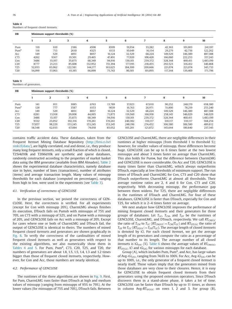
contains traffic accident data. These databases, taken from theFrequent Itemset Mining Database Repository (http://fimi.cs.helsinki.fi/data/), are highly correlated, real and dense, i.e., they producemany long frequent itemsets, only a small fraction of which is closed.T25i4d10k and T20i6d10k are synthetic and sparse databases,randomly constructed according to the properties of market basketdata using the IBM generator (available from IBM Almaden). Table 2shows the experimental database characteristics, namely databasesize in bytes, number of lines (transactions), number of attributes(items) and average transaction length. Many values of minsuppthresholds for each database (computed on percentages), rangingfrom high to low, were used in the experiments (see Table 3).

4.1. Verification of correctness of GENCLOSE

In the previous section, we proved the correctness of GEN-CLOSE. Here, the correctness is verified. For all experiments(except for Con with minsupp 20%), CharmLMG always finishesits execution, DTouch fails on Pumsb with minsupps of 75% and70%, on C73 with a minsupp of 52%, and on Pumn with a minsuppof 20%, and GENCLOSE fails on Acc with a minsupp of 20%. Exceptfor cases where one or both of CharmLMG and DTouch fail, theoutput of GENCLOSE is identical to theirs. The numbers of minedfrequent closed itemsets and generators are shown graphically inFig. 8. To verify the correctness of the cardinalities of minedfrequent closed itemsets as well as generators with respect tothe existing algorithms, we also numerically show them inTables 4 and 5. For Pum, Pumn, C73, C20, T25, and T20, thenumbers of generators are about 1.8, 1.5, 1.5, 1.4, 1.3 and 1.2 timesbigger than those of frequent closed itemsets, respectively. How-ever, for Con and Acc, those numbers are nearly identical.

4.2. Performance of GENCLOSE

The runtimes of the three algorithms are shown in Fig. 9. First,for Pum, CharmLMG runs faster than DTouch at high and mediumvalues of minsupp (ranging from minsupps of 95% to 79%). At thelower values (for minsupps of 75% and 70%), DTouch fails. Between

GENCLOSE and CharmLMG, there are negligible differences in theirruntimes at higher minsupps (from threshold 1 to threshold 5);however, for smaller values of minsupp, those differences becomehuge. GENCLOSE can be up to 6 times faster at the two lowestminsupps and about 3 times faster on average than CharmLMG.This also holds for Pumn, but the difference between CharmLMGand GENCLOSE is more considerable. On Acc and T20, GENCLOSE ismany times faster than CharmLMG, which always outperformsDTouch, especially at low thresholds of minimum support. The runtimes of DTouch and CharmLMG for Con, C73 and C20 show thatDTouch outperforms CharmLMG at almost all thresholds. Theiraverage runtime ratios are 2, 4 and 6 for Con, C73 and C20,respectively. With decreasing minsupp, the performance gapbetween them widens. For T25, there are negligible differencesin the runtimes of DTouch and CharmLMG. For four of thesedatabases, GENCLOSE is faster than DTouch, especially for Con andT25, for which it is 2–4 times faster on average.

We next analyze how GENCLOSE improves the performance ofmining frequent closed itemsets and their generators for threegroups of databases. Let TGC, TCM, and TDT be the runtimes ofGENCLOSE, CharmLMG, and DTouch, respectively. We call RTCM/GC

the ratio of TCM to TGC (RTCM/GC:¼TCM/TGC) and RTDT/GC the ratio ofTDT to TGC (RTDT/GC:¼TDT/TGC). The average length of closed itemsetsis denoted by |C|. For each closed itemset, we get the averagelength of its generators and compute the ratio as a percentage ofthat number to its length. The average number of all closeditemsets is |G|||/|C| (%). Table 6 shows the average values of RTCM/GC,RTDT/GC, |C| and |G|||/|C| for various minsupps for each database.

Group (A), which includes Pum, Pumn, and Acc, has large valuesof Avg-|G|||/|C|, ranging from 74.6% to 100%. For Acc, Avg-|G|||/|C| can beup to 100%, i.e., the only generator of a frequent closed itemset isnearly itself. Those values imply that the generators mined fromthose databases are very close to their closures. Hence, it is easyfor GENCLOSE to obtain frequent closed itemsets from theirgenerators using the proposed extension operators. Since DTouchdiscovers them in a stand-alone phase, it takes a lot of time.GENCLOSE can be faster than DTouch by up to 11 times, as shownin column Avg-RTDT/GC on rows 1, 2 and 3. For group (B),

Table 4Numbers of frequent closed itemsets.


1 2 3 4 5 6 7 8 9 10

Pum 110 610 2186 4508 8509 19,934 33,282 42,363 101,003 241,197Pumn 116 713 2610 4325 6133 10,649 16,154 29,279 42,756 122,262Acc 149 529 4051 8057 16,124 32,529 68,224 149,529 346,389 887,388C73 4262 9367 19,501 29,465 47,491 77,920 108,428 166,060 222,253 357,243Con 3486 15,107 35,875 68,349 94,916 130,101 239,372 328,344 460,411 1,483,199C20 8777 21,213 85,608 132,952 151,394 177,195 218,455 292,523 316,412 340,468T25 52,033 83,062 122,581 144,177 163,625 184,300 200,666 221,074 221,074 343,733T20 54,099 57,063 61,185 66,899 75,743 90,501 101,895 117,344 139,469 171,796

Table 5Numbers of generators.


1 2 3 4 5 6 7 8 9 10

Pum 141 811 3085 6763 13,789 37,023 67,810 90,252 248,170 658,380Pumn 128 777 3587 6153 9039 16,763 26,971 51,800 78,219 253,240Acc 149 529 4051 8057 16,124 32,529 68,224 149,529 346,389 887,388C73 6281 13,918 29,008 44,065 71,875 119,560 166,918 258,145 346,029 346,029Con 3486 15,107 35,875 68,349 94,916 130,101 239,372 328,344 460,411 1,483,199C20 9332 23,052 102,316 170,261 170,261 240,382 310,117 310,117 310,117 568,254T25 57,857 98,229 153,245 153,245 153,245 248,196 274,452 306,580 306,580 489,812T20 58,548 62,035 67,084 74,018 85,052 105,281 121,872 145,644 180,840 237,345


http://fimi.cs.helsinki.fi/data/

http://fimi.cs.helsinki.fi/data/

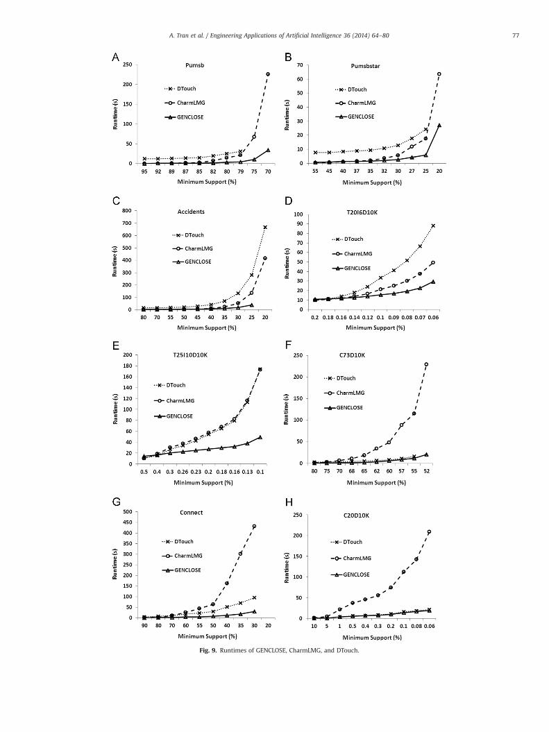
Fig. 9. Runtimes of GENCLOSE, CharmLMG, and DTouch.


GENCLOSE has difficulty when trying to reach long frequent closeditemsets that are much longer than their generators. However, it isstill about 3 or 4 times faster than DTouch (except on C20, wheretheir performance difference is only 1.2 times).

Now, let us compare GENCLOSE to CharmLMG. For group (A),which produces short frequent closed itemsets, the mining ofgenerators with short lengths by MinimalGenerator is fast. Hence,the total runtimes of CharmLMG are similar to those of GENCLOSE(see first three rows in column Avg-RTCM/GC). For group (B), thetime for checking the sufficient condition for generators based onlong frequent closed itemsets is longer. CharmLMG is up to7.8 times (on average) slower than GENCLOSE.

The synthetic databases T25i4d10k and T20i6d10k are sparseand thus produce very short frequent closed itemsets (withaverage lengths of 5.0 and 4.1, respectively, as shown in Table 6).For this group, the performances of three algorithms are similar.However, GENCLOSE is still about 2 times faster.

5. Conclusions and future works

This study described the properties of closed sets and gen-erators as well as their relations. The necessary and sufficientconditions to produce generators and operators to determineclosed itemsets were derived. The GENCLOSE algorithm wasproposed for simultaneously mining frequent closed itemsetsand their generators. Using the IOG-tree framework, it uses theitemset object-set and generator space, which allow not only quickidentification of new generators without accessing the database ortesting mined generators, but also extension of pre-closed item-sets toward their closures. Experiments on real and syntheticbenchmark datasets confirm that GENCLOSE significantly outper-forms existing methods in mining frequent closed itemsets andgenerators.

For mining either closed itemsets or generators separately,depth-first algorithms usually outperform level-wise ones. Aninteresting extension is to develop a depth-first miner based onour approach. Further, to deal with large databases, it is necessaryto convert GENCLOSE for parallel and distributed environments aswell as to execute different mining tasks, such as sequence mining.

Acknowledgment

This work was funded by the National Foundation for Scienceand Technology Development (NAFOSTED) under Grant no.102.05-2013.20.

Appendix A. Proofs

Proposition 1. Proof. Here, we only prove property 5.(b).

“) ” Since ρ(A1)Cρ(A2), h(A1)¼λ(ρ(A1))+λ(ρ(A2))¼h(A2). Ifh(A1)¼h(A2), using 5.(a), ρ(A1)¼ρ(A2). This is a contradiction.Hence, h(A1)*h(A2).“( ” Since h(A1)*h(A2), using the anti-monotone law of ρ, ρ(h(A1))¼ρ(A1)Dρ(h(A2))¼ρ(A2). If ρ(A2)¼ρ(A1), then h(A1)¼h(A2) (from 5.(a)). This implies that ρ(A2)*ρ(A1). □

Consequence 1. Proof.

1) (a) “) ” (b): For every P*A¼h(A), we always have ρ(A)+ρ(P)and supp(A)Z supp(P). Now, let us assume that supp(A)¼supp(P). Thus, ρ(A)¼ρ(P) and P*A¼h(A)¼h(P)+P. This implies acontradiction. Hence, supp(A)4supp(P).(b) “) ” (c): For every P*A, ρ(A)+ρ(P). If ρ(A)¼ρ(P), thensupp(A)¼supp(P). It is a contradiction. Thus, ρ(A)*ρ(P).(a) “( ” (c): We have ADh(A) and ρ(A)¼ρ(h(A)). If ACh(A),then we take P� h(A), ρ(A)*ρ(P)¼ρ(h(A)): a contradiction.Hence, A¼h(A).

2) For closed itemset h(A), we have h(A)+A, ρ(A)¼ρ(h(A)), supp(A)¼supp(h(A)), h(A)¼h(h(A)).(a) As follows from property 5 of Proposition 1 and Remark 1,we have for every Q*P: h(Q)*h(P) 3 ρ(Q)Cρ(P) 3 supp(Q)osupp(P) and if P+A, then h(A)¼h(P) 3 ρ(A)¼ρ(P) 3 supp(A)¼supp(P). What is left is to prove that the closure of A is theunique set P such that

P+A;hðPÞ ¼ hðAÞ and ðhðQ Þ*hðPÞ; 8Q*PÞ ð14Þ

þ Clearly, h(A) satisfies (14): h(A)¼h(h(A))+A and (8 Q*h(A),h(Q)+h(A)). If h(A)¼h(Q), Q*h(A)¼h(Q)+Q. This is a contra-diction. Therefore, h(Q)*h(A)¼h(h(A)).þ Wewill show the fact that for P satisfying (14), P¼h(A). Sinceh(A)¼h(P)+P+A, if ADPCh(A), we take Q¼h(A)*P+A.Thus,

hðAÞ ¼ hðQ Þ*hðPÞ ð15Þ

Otherwise, h(A)¼h(h(A))+h(P)+h(A) implies that h(A)¼h(P).This contradicts (15). Hence, P¼h(A) is unique.(b) Obviously, the closure h(A) is the superset of A whichsatisfies (1). For every B+A, from properties of 2 and 5 ofProposition 1 and Remark 1, the conditions in (1) are equiva-lent, i.e., supp(A)¼supp(B) 3 ρ(A)¼ρ(B)3h(A)¼h(B). Then,we only need to prove that h(A) is the maximum superset of Asuch that h(A)¼h(B). Conversely, assume that there exists B*h(A)such that B is a superset of Awith h(A)¼h(B). Thus, B*h(A)¼h(B)+B. This is a contradiction. Thus, the closed set h(A) is themaximum superset of A satisfying (1).

3) It is easy to see that h(A) is a closed itemset containing A. Let Bbe a closed itemset containing A, i.e., B¼h(B)+A. By themonotone and idempotence properties, we have B¼h(B)¼h(h(B))+h(A). Therefore, h(A) is a minimum closed itemsetcontaining A with the set containment order “D”. □

Consequence 2. Proof.The equivalence (a)3(b) comes naturally from property 5 of

Proposition 1. Based on Remark 1 and the fact that [GDA)ρ(G)+ρ(A)], we have (a)3(c).

This proof is deduced from the above statement since h(G)¼h(h(G)), ρ(G)¼ρ(h(G)) and supp(G)¼supp(h(G)). □

Proposition 2. Proof.Assuming that A

��¼m. Let us finitely consider the subsets of A,

each of which is created by deleting an item of A: Ai1 ¼ Anfai1 g; ai1 AA; 8 i1 ¼ 1…m:

Table 6Performance of GENCLOSE compared to CharmLMG and DTouch.

Group DB Avg-|C| Avg-|G|||/|C| (%) Avg-RTCM/GC Avg-RTDT/GC

(A) Pum 6.0 90.0 3.2 11.7Pumn 6.7 74.6 1.6 6.5Acc 5.3 100.0 1.6 6.2

(B) C73 10.7 59.9 7.9 2.9Con 12.1 47.3 8.3 4.3C20 10.4 49.6 7.2 1.2

(C) T25 5.0 85.8 2.0 1.9T20 4.1 92.8 1.3 1.9


Case 1: If ρ(Ai1 )*ρ(A), 8 i1 ¼ 1…m, then A is a generator of A.Case 2: Otherwise, there exists i1 ¼ 1…m: ρ(Ai1 )¼ρ(A). Theabove steps are repeated for Aij (j¼ 1…m�1) until:case 1 happens thus, we get the generator Aij� 1

of A; orcase 2 happens when jAim� 1

j ¼ 1; i:e:; rðAi1 Þ ¼ rð Ai2 Þ ¼⋯¼ρð Aim� 1

Þ ¼ ρðAÞ. Hence, Aim� 1is a generator of A. Since A is finite,

we always discover a generator of A.

GAG(A) 3 [GDA, h(G)¼h(A) and (h(G0)Ch(G),8G0:∅aG0CG)]. Furthermore, for every B+A such that h(A)¼h(B).Then, GAG(A) implies that [GDB, h(G)¼h(B) and (h(G0)Ch(G),8G0: ∅aG0CG)], i.e., GAG(B). Thus, G(A)DG(B).

“) ”: If GA⌊Ac is a generator of A but not minimal in ⌊Ac, thereexists G0A⌊Ac such that ∅aG0CG. Hence, h(G0)¼h(A). This con-tradicts the fact that G is a generator.

“( ”: Let us consider a minimal element G of ⌊Ac. We have∅aGDA, h(G)¼h(A). Further, for every proper subset G0 of G, wehave: h(G0)Ch(G), 8G0: ∅aG0CG. Since G0CG, then h(G0)Dh(G).If h(G0)¼h(G), i.e., G0 is in ⌊Ac. Therefore, G is not minimal. This is acontradiction. Hence, G is a generator of A. □

Appendix B. Implemented techniques

Fast implementation based on diffsets. In order to reducememory, the diffset technique is used in many algorithms, such asCharm, Eclat, and Touch. It is thus applied in GENCLOSE. Instead ofstoring whole object-sets, we only store the corresponding diff-sets. A diffset at each node keeps track of its object-set from thediffsets of its left-most ancestors. The diffset of node Nk at L[k](with kZ1) is defined as the difference between its object-set andthe object-set of its left-parent Left at L[k�1], i.e.:

dðNk; Lef tÞ : ¼ ρðLef t:HÞ n ρðNk:HÞSince this difference is insignificant in comparison with the

object-set size, the memory required is considerably reduced. As

convention, the unique left-parent of all nodes in L[1] is Root withρ(Root)¼{a AA: sup({a})Z minsupp}. For example, the differ-ences for nodes G, B, E, H, and C are {2, 5, 6}, {2, 3}, {2, 6}, {5, 6},and {3}, respectively (see Fig. 11). For k41, let (Left, Right) be thepair that produces Nk and LP be their common left-parent. It iseasy to find that (see Fig. 10):

dðNk; Lef tÞ ¼ dðRight; LPÞ n dðLef t; LPÞ ð16Þ

Nk:Supp¼ Lef t:Supp–jdðNk; Lef tÞj ð17ÞObserving folder G in Fig. 7, we notice that GB comes from not

only left-parent G but also from B (since we merged BH to GB).Hence, GB contains two diffsets, {3} and {5, 6}. In general, a node Nwith a diffset is obtained in the form (SuppH, {[Left-parentj, d(N,Left-parentj), GSj]}), where GSj is the set of generators generatedfrom Left-parentj (jth left-parent), j¼1, 2, … For instance, GB¼(2eghbc, {[G, {3}, {gb, gc}], [B, {5,6}, {bh}]}) (see Fig. 11).

Let us consider the execution of ExtendMerge with diffsets. Iftwo nodes Left and Right have the same left-parent LP, the relationof the two respective diffsets implies that of two object-sets:

dðLef t; LPÞDdðRight; LPÞ3ρðLef t:HÞ+ρðRight:HÞOtherwise, their pre-closed itemsets share the same object-set

only for:

ðLef t:HDRight:H or Right:HDLef t:HÞ and Lef t:Supp¼ Right:Supp

For example, we merge GC to GB since d(GC, G)¼d(GB, G), but,BH to GB since (BH.HCGB.H and BH.Supp¼GB.Supp). In the secondphase, for the combination of the two nodes Left and Right, weneed to locate their shared left-parent. If it does not exist, thesenodes cannot be joined together. Otherwise, let LP be that left-parent. We compute NewDiff (instead of NewO) based on the twocorresponding diffsets and then NewSupp using (16) and (17). InJoinForGenerators, we consider only the generator pairs (Gl, Gr)such that Gl and Gr have the same left-parent. For instance, for (GB,BE): LP¼B, NewDiff¼∅. Thus, NewSupp¼2 does not pass the teston Line 11. For (BE, EH), we consider the generator pair of ce and eh

Fig. 10. Diffset computation.

Fig. 11. Execution of GENCLOSE with diffsets.


since their common left-parent is E. Since there exists G¼ceh, itpasses the tests on Lines 27 and 28 and new node BEH is created.See Fig. 11 for the execution of GENCLOSE with diffsets.

Fast searching onℒCG using a doublehash. In order to reach theclosures using operator EOC, we need to quickly search ℒCG forclosure P of itemset hG. Obviously, a search based only on thesupport (supp(hG)) or/and the itemset (hG) is not efficient. As theobject-set shared an itemset is identical to the one shared itsclosure, using the information about the known object-set (OG) todetermine the closure of an itemset helps reduce the search timeconsiderably. We first apply the hash technique based on the sumof object-sets (proposed by Zaki and Hsiao (2005)). Since we storeonly diffsets and not object-sets, the sum should be computedthrough diffsets. More formally, let Nk be a new node with left-parent Left. Its object-set sum, called Nk.SumO, is computed by

Nk:SumO¼ Lef t:SumO� ∑mAdðNk ;LPÞ

m

Since many closures can have the same hash value (based onthe sum of objects), we hash them later by the support. Once anitemset hG passes the tests on the hash values based on the object-set sum and support, we check the support and set containmentrelation to locate its closure.

References

Agrawal, R., Imielinski, T., Swami, N., 1993. Mining association rules between sets ofitems in large databases. In: Proceedings of the ACM SIGMOID 1993, pp. 207–216.

Agrawal, R., Srikant, R., 1994. Fast algorithms for mining association rules. In:Proceedings of the 20th International Conference on Very Large Data Bases,pp. 478–499.

Anh, T., Hai, D., Tin, T., Bac, L., 2011. Efficient algorithms for mining frequentitemsets with constraint. In: Proceedings of the 3rd International Conferenceon Knowledge and System Engineering KSE 2011, pp. 19–25.

Anh, T., Tin, T., Bac, L., 2012a. Structures of association rule set. In: Proceedings ofACIIDS 2012, LNAI 7197, Part II. Springer-Verlag, pp. 361–370.

Anh, T., Hai, D., Tin, T., Bac, L., 2012b. Mining frequent itemsets with dualisticconstraints. In: Proceedings of PRICAI 2012, LNAI 7458. Springer-Verlag,pp. 807–813.

Anh, T., Tin, T., Bac, L., 2013. An approach for mining concurrently closed itemsetsand generators. Adv. Comput. Methods Knowl. Eng. SCI 479, 355–366.

Anh, T., Tin, T., Bac, L., 2014. An approach for mining association rules intersectedwith constraint itemsets. Adv. Intell. Syst. Comput. 245, 351–363.

Balcazar, J.L., 2010. Redundancy, deduction schemes, and minimum-size base forassociation rules. Log. Methods Comput. Sci. 6 (2:3), 1–33.

Bastide, Y., Taouil, R., Pasquier, N., Stumme, G., Lakhal, L., 2000. Mining frequentpatterns with counting inference. SIGKDD Explor. 2 (2), 66–75.

Bay, V., Hong, T.P., Bac, L., 2012. Mining most generalization association rules basedon frequent closed itemset. Int. J. Innov. Comput., Inform. Control 8 (10), 1–17.

Bayardo, R.J., 1998. Efficiently mining long patterns from databases. In: Proceedingsof the SIGMOD Conference 1998, pp. 85–93.

Birkhoff, G., 1967. Lattice Theory, 3rd edition American Mathematical Society,Providence, RI.

Boulicaut, J., Bykowski, A., Rigotti, C., 2003. Free-Sets: a condensed representationof boolean data for the approximation of frequency queries. Data Min. Knowl.Discov. 7, 5–22.

Burdick, D., Calimlim, M., Gehrke, J., 2001. MAFIA: a maximal frequent itemsetalgorithm for transactional databases. In: Proceedings of ICDE’01, pp. 443–452.

Davey, B.A., Priestley, H.A., 1994. Introduction to Lattices and Order, fourth editionCambridge University Press, Cambridge.

Dong, G., Jiang, C., Pei, J., Li, J., Wong, L., 2005. Mining succinct systems of minimalgenerators of formal concepts. In: Proceedings of DASFAA 2005, LNCS 3453,pp. 175–187.

Ganter, B., Wille, R., 1999. Formal Concept Analysis: mathematical foundations.Springer-Verlag.

Hai, D., Tin, T., Bac, L., 2013. An efficient algorithm for mining frequent itemsetswith single constraint. Adv. Comput. Methods Knowl. Eng. SCI 479, 367–378.

Hai, D., Tin, T., Bac, L., 2014. An efficient method for mining frequent itemsets withdouble constraints. J. Eng. Appl. Artif. Intell. 27, 148–154.

Han, J., Pei, J., 2000. Mining frequent patterns by pattern-growth: methodology andimplications. ACM SIGKDD Explor. 2 (2), 14–20.

Han, J., Pei, J., Yin, J., Mao, R., 2004. Mining frequent patterns without candidategeneration: a frequent-pattern tree approach. Data Min. Knowl. Discov. 8 (1),53–87.

Hashem, T., Ahmed, C.F., Samiullah, M., Akther, S., Jeong, B.-S., Jeon, S., 2014. Anefficient approach for mining cross-level closed itemsets and minimal associa-tion rules using closed itemset lattices. Expert Syst. Appl. 41 (6), 2914–2938.

Pasquier, N., Bastide, Y., Taouil, R., Lakhal, L., 1999. Efficient mining of associationrules using closed item set lattices. Inf. Syst. 24 (1), 25–46.

Pasquier, N., Taouil, R., Bastide, Y., Stumme, G., Lakhal, L., 2005. Generating acondensed representation for association rules. J. Intell.t Inf. Syst. 24 (1), 29–60.

Pei, J., Han, J., Mao, R., 2000. CLOSET: an efficient algorithm for mining frequentclosed itemsets. In: Proceedings of the DMKDWorkshop on Research Issues inData Mining and Knowledge Discovery 2000, pp. 21–30.

Singh, N.G., Singh, S.R., Mahanta, A.K., 2005. CloseMiner: discovering frequentclosed itemsets using frequent closed tidsets. In: Proceedings. of the 5th ICDM,Washington DC, USA, pp. 633–636.

Szathmary, L., Valtchev, P., Napoli, A., 2009. Efficient vertical mining of frequentclosed itemsets and generators. In: Proceedings of IDA 2009, pp. 393–404.

Tin, T., Anh, T., 2010a. Structure of set of association rules based on concept lattice.In: Proceedings of ACIIDS 2010, Advanced in Intelligent Information andDatabase Systems, SCI 283, Springer, pp. 217–227.

Tin, T., Anh, T., Thong, T., 2010b. Structure of association rule set based on min-minbasic rules. In: Proceedings of the International Conference on Computing andCommunication Technologies RIVF 2010, pp. 83–88.

Zaki, M.J., 2000. Scalable algorithms for association mining. IEEE Trans. Knowl. DataEng. 12 (3), 372–390.

Zaki, M.J., Gouda, K., 2003. Fast vertical mining using diffsets. In: Proceedings of the9th ACM SIGKDD.

Zaki, M.J., 2004. Mining non-redundant association rules. Data Min. Knowl. Discov.9, 223–248.

Zaki, M.J., Hsiao, C.J., 2005. Efficient algorithms for mining closed itemsets and theirlattice structure. IEEE Trans. Knowl. Data Eng. 17 (4), 462–478.

Vo, B., Le, B., 2009. Fast algorithm for mining minimal generators of frequent closeditemsets and their applications. In: Proceedings of 39th International Con-ference on Computers and Industrial Engineering, pp. 1407–1411.

Wang, J., Han, J., Pei, J., 2003. Closetþ: searching for the best strategies for miningfrequent closed itemsets. In: Proceedings of ACM SIGKDD’03.

Wille, R., 1982. Restructuring lattices theory: an approach based on hierarchies ofconcepts. In Ordered Sets, pp. 445–470.

Wille, R., 1992. Concept lattices and conceptual knowledge systems. Comput. Math.Appl. 23, 493–515.


http://refhub.elsevier.com/S0952-1976(14)00171-7/sbref1











































simultaneous mining of frequent closed itemsets and their generators: foundation and algorithm

Documents