simultaneous conversions with the residue number system ...lebreton/fichiers/doliskani, giorgi,...

1

Simultaneous Conversions with the Residue Number System usingLinear Algebra

JAVAD DOLISKANI, Institute for antum Computing, University of Waterloo

PASCAL GIORGI, LIRMM CNRS - University of Montpellier

ROMAIN LEBRETON, LIRMM CNRS - University of Montpellier

ERIC SCHOST, University of Waterloo

We present an algorithm for simultaneous conversions between a given set of integers and their Residue

Number System representations based on linear algebra. We provide a highly optimized implementation of

the algorithm that exploits the computational features of modern processors. e main application of our

algorithm is matrix multiplication over integers. Our speed-up of the conversions to and from the Residue

Number System signicantly improves the overall running time of matrix multiplication.

CCS Concepts: •Mathematics of computing →Mathematical soware performance; Computationsin nite elds; Computations on matrices; •eory of computation →Design and analysis of algo-rithms;

ACM Reference format:Javad Doliskani, Pascal Giorgi, Romain Lebreton, and Eric Schost. 2016. Simultaneous Conversions with

the Residue Number System using Linear Algebra. ACM Trans. Math. Sow. 1, 1, Article 1 (January 2016),

21 pages.

DOI: 10.1145/nnnnnnn.nnnnnnn

1 INTRODUCTIONere currently exist a variety of high-performance libraries for linear algebra or polynomial

transforms which use oating-point arithmetic (Frigo and Johnson 2005; Goto and van de Geijn

2008; Puschel et al. 2005; Whaley et al. 2001), or computations over integers or nite elds (Bosma

et al. 1997; Dumas et al. 2008; Hart 2010; Shoup 1995).

In this paper, we are interested in the laer kind of computation, specically in the context

of multi-precision arithmetic. Suppose for instance we deal with matrices or polynomials with

coecients that are multi-precision integers, or lie in a nite ring Z/NZ for some large N , and

consider a basic operation such as the multiplication of these matrices or polynomials (there exist

multiple applications for this fundamental operation; some of them are illustrated in Section 4.3).

To perform a matrix or polynomial multiplication in such a context, several possibilities exist.

A rst approach consists in applying known algorithms, such as Strassen, Karatsuba, . . . directly

over our coecient ring, relying in ne on fast algorithms for multiplication of multi-precision

integers. Another large class of algorithms relies on modular techniques, or Residue Number Systems,computing the required result modulo many small primes before recovering the output by Chinese

Remaindering. Neither of these approaches is superior in all circumstances. For instance, in extreme

cases such as the product of matrices of small size and large integer entries, the modular approach

Permission to make digital or hard copies of all or part of this work for personal or classroom use is granted without fee

provided that copies are not made or distributed for prot or commercial advantage and that copies bear this notice and

the full citation on the rst page. Copyrights for components of this work owned by others than ACM must be honored.

Abstracting with credit is permied. To copy otherwise, or republish, to post on servers or to redistribute to lists, requires

prior specic permission and/or a fee. Request permissions from [email protected].

© 2016 ACM. 0098-3500/2016/1-ART1 $15.00

DOI: 10.1145/nnnnnnn.nnnnnnn

ACM Transactions on Mathematical Soware, Vol. 1, No. 1, Article 1. Publication date: January 2016.

1:2 Javad Doliskani, Pascal Giorgi, Romain Lebreton, and Eric Schost

highlighted above is most likely not competitive with a direct implementation (see (Harvey and

Hoeven 2014) for a review of best current complexities for integer matrix multiplication). On the

other hand, for the product of larger matrices (or polynomials), Residue Number Systems oen

perform beer than direct implementations (see Section 4.2), and as such, they are used in libraries

or systems such as NTL, FFLAS-FFPACK, Magma, . . .

In many cases, the bolenecks in such an approach are the reduction of the inputs modulo many

small primes, and the reconstruction of the output from its modular images by means of Chinese

Remaindering; by contrast, operations modulo the small primes are oen quite ecient. Algo-

rithms of quasi-linear complexity have been long known both for modular reduction and Chinese

Remaindering (Borodin and Moenck 1974), based on so-called subproduct tree techniques; however,

their practical performance remains somewhat slow. In this paper, we propose an alternative to

these algorithms, appropriate for those cases where we have several coecients to convert; it

relies on matrix multiplication to perform these tasks, with matrices that are integer analogues of

Vandermonde matrices and their inverses. As a result, while their asymptotic complexity is inferior

to that of asymptotically fast methods, our algorithms behave extremely well in practice, as they

allow us to rely on high-performance libraries for matrix multiplication.

Finally we give a glimpse of performance implications our improved matrix multiplication algo-

rithm can yield to many algorithms. We will focus on the problems of modular composition, power

projection, minimal polynomial and factorization. By plugging our multi-precision integer matrix

multiplication algorithm into NTL existing implementations, we are able to show a substantial gain

in performance.

Organization of the paper. We rst give an overview of the Residue Number System and its

classical algorithms in Section 2. In Section 3, we discuss algorithms for converting simultaneously

a given set of integers to their Residue Number System representation, and vice versa. We contribute

by giving a new algorithm based on linear algebra in Sections 3.1 and 3.2, and we report on our

implementation inside FFLAS-FFPACK in Section 3.3. We then use these results to implement an

ecient integer matrix multiplication algorithm in Section 4 and report on direct performance

improvement of sample applications in Section 4.3. Finally, we extend our algorithms to larger

moduli in Section 5 and we report on our implementation in Section 5.5.

2 PRELIMINARIES2.1 Basic resultsOur computation model is that of (Gathen and Gerhard 2013, Chapter 2) or (Brent and Zimmermann

2010, Chapter 1.1): we x a base β , that can typically be a power of two such as 2, 216or 2

32, and

we assume that all non-zero integers are wrien in this basis: such an integer a is represented by

coecients (a0, . . . ,as−1), with each ai in 0, . . . , β − 1 and as−1 non-zero, together with a sign bit,

such that a = ±(a0 + a1β + · · · + as−1βs−1). e coecients ai are referred to as words; the integer s

is called the length of a, and denoted by λ(a).Our complexity statements are given in terms of the number of operations on words, counting

each operation at unit cost (for the details of which operations are used, see (Gathen and Gerhard

2013, Chapter 2)). For simplicity, we assume that all words can also be read or wrien in O(1) such

that our complexity estimates t the standard word RAM model (Hagerup 1998). We let I : N→ Nbe such that two integers a,b of length at mostn can be multiplied in I(n)word operations, assuming

the base-β expansions of a andb are given; we assume that I satises the super-linearity assumptions

of (Gathen and Gerhard 2013, Chapter 8). One can take I(n) in n log(n)2O(log∗(n))

using Fast Fourier

Transform techniques (Furer 2007; Harvey et al. 2016).


Simultaneous Conversions with the Residue Number System using Linear Algebra 1:3

We will oen use the fact that given integers a,b of lengths respectively n and t , with t 6 n, one

can compute the product ab using O(n I(t)/t) word operations: without loss of generality, assume

that a and b are positive and write a in base β t as a = a0 + a1βt + · · · + a`β`t , with ` ∈ Θ(n/t), so

that ab = (a0b) + (a1b)β t + · · · + (a`b)β`t . Writing a as above requires no arithmetic operation;

the coecients ai are themselves wrien in base β . All coecients aib can be computed in time

O(` I(t)) = O(n I(t)/t). Since aib < β2t

holds for all i , going from the above expansion to the base-βexpansion of ab takes time O(n), which is O(n I(t)/t).

For m ∈ N>0, we write Z/mZ for the ring of integers modulo m. We denote by respectively

(a rem m) and (a quo m) the remainder and quotient of the Euclidean division of a ∈ Z bym ∈ N>0,

with 0 6 (a rem m) < m; we extend the notation (a rem m) to any rational a = n/d ∈ Q such that

gcd(d,m) = 1 to be the unique b in 0, . . . ,m − 1 such that bd ≡ n (mod m).Let a ∈ Z and m ∈ N>0 be of respective lengths at most n and t , with t 6 n. en, one can

compute the quotient (a quo m) and the remainder (a rem m) using O(I(n)) word operations;

the algorithm goes back to (Cook 1966), see also (Aho et al. 1974, Section 8.2) and (Brent and

Zimmermann 2010, Section 2.4.1). In particular, arithmetic operations (+,−,×) in Z/mZ can all

be done using O(I(t)) word operations; inversion modulom can be done using O(I(t) log(t)) word

operations.

More rened estimates for Euclidean division are available in some cases:

• Consider rst the case where n t . Given a and m as above, we can compute both

(a quo m) and (a rem m) using

O(I(t)tn

)(1)

word operations. To do so, write a in base β t as a = a0+a1βt + · · ·+a`β`t , with ` ∈ Θ(n/t);

this does not involve any operations, since a is given by its base-β expansion. Dene

q`+1 = r`+1 = 0, and, for i = `, . . . , 0, ri = (β tri+1+ai ) rem m and qi = (β tri+1+ai ) quo m.

is computes r0 = (a rem m), and we get q = (a quo m) as q = q0 + q1βt + · · · + q`β`t

(which produces its base-β expansion without any further work). e total time of this

calculation is as in (1).

• Finally, if we suppose more precisely that β t−1 6 m < β t , in cases where n − t 6 t , the

remainder (a rem m) can be computed in time

O(I(n − t)n − t t

). (2)

Indeed, in this case, the quotient q = (a quo m) can actually be computed in O(I(n − t))word operations, since λ(q) is in O(n − t) (see (Giorgi et al. 2013, Algorithm 2)). Once qis known, one can compute qm in time O(t I(n − t)/(n − t)), as explained above; deducing

(a rem m) takes another O(t) word operations, hence the cost claimed above.

We also let MM : N3 → N be such that one can do integer matrix multiplication for matrices of

size (a,b) × (b, c) using MM(a,b, c) operations (+,−,×) in Z, with an algorithm that uses constants

bounded independently of a,b, c . e laer requirement implies that for any m > 0, with m of

length t , one can do matrix multiplication in size (a,b) × (b, c) over Z/mZ using O(MM(a,b, c) I(t))word operations. is also implies that given integer matrices of respective sizes (a,b) and (b, c),if the entries of the product are bounded by β t in absolute value, one can compute their product

using O(MM(a,b, c) I(t)) word operations, by computing it modulo an integer of length Θ(t).Let ω be such that we can multiply b × b integer matrices using O(bω ) operations in Z, under

the same assumption on the constants used in the algorithm as above; the best known bound on ω



is ω < 2.3729 (Coppersmith and Winograd 1990; Le Gall 2014; Stothers 2010; Vassilevska Williams

2012). So MM(b,b,b) = O(bω ) and MM(a,a,b) = O(aω−1b)when a 6 b by partitioning into square

blocks of size a.

2.2 The Residue Number Systeme Residue Number System (RNS) is a non-positional number system that allows one to represent

nite sets of integers. Letm1,m2, . . . ,ms ∈ N be pairwise distinct primes, and let

M =m1m2 · · ·ms .

en any integer a ∈ 0, . . . ,M − 1 is uniquely determined by its residues ([a]1, [a]2, . . . , [a]s ),with [a]i = (a rem mi ); this residual representation is called a Residue Number System.

Operations such as addition and multiplication are straightforward in the residual representation;

however, conversions between the binary representation of a and its residual one are potentially

costly. For the following discussion, we assume that allmi ’s have length at most t ; in particular,

any a in 0, . . . ,M − 1 has length at most st .e conversion to the RNS representation amounts to taking a as above and computing all

remainders (a rem mi ). Using (1), we can compute each of them in O(s I(t)) word operations,

for a total time in O(s2I(t)). A divide-and-conquer approach (Borodin and Moenck 1974) leads

to an improved estimate of O(I(st) log(s)) word operations (see also (Gathen and Gerhard 2013,

eorem 10.24)). Note that (Bernstein 2004) gives a constant improvement of this algorithm.

e inverse operation is Chinese Remaindering. Let a be an integer in 0, . . . ,M − 1 given by

its RNS representation ([a]1, . . . , [a]s ); then, a is equal to[s∑i=1

([a]iui rem mi )Mi

]rem M, (3)

where we write Mi = M/mi and ui = (1/Mi rem mi ) for all i .From this expression, one can readily deduce an algorithm of cost O(s2 I(t) + s I(t) log(t)) to

compute a. One rst computes M in the direct manner, by multiplying 1 by successivelym1, . . . ,ms ;

the total time isO(s2 I(t))word operations. From this, allMi ’s can be deduced in the same asymptotic

time, since we saw in the previous section that one can compute (M quo mi ) in time O(s I(t)) for all

i . One can further compute all remainders (Mi rem mi ) in time O(s2 I(t)) by the same mechanism.

Deducing all ui ’s takes O(s I(t) log(t)) word operations, since we do s modular inversions with

inputs of length at most t . One can then deduce a by simply computing all summands in (3)

and adding them (subtracting M whenever a sum exceeds this value), for another O(s2 I(t)) word

operations. e total time is thus O(s2 I(t) + s I(t) log(t)) word operations.

To do beer, consider the mapping

φ : (v1, . . . ,vs ) 7→s∑i=1

viMi rem M,

withvi in 0, . . . ,mi−1 for all i . Using the divide-and-conquer approach from (Borodin and Moenck

1974) (see also (Gathen and Gerhard 2013, Algorithm 10.20)), φ(v1, . . . ,vs ) can be computed in

O(I(st) log(s)) word operations (taking care to reduce all results, whenever required). In particular,

(Mi rem mi ) can be computed as (φ(1, . . . , 1) rem mi ), so all of them can be deduced in time

O(I(st) log(s)); as above, we deduce all ui ’s using an extra O(s I(t) log(t)) operations. Once they

are known, the computation of a = φ(a1u1, . . . ,asus ) from its residuals is reduced to s modular

multiplications of length t , and an application ofφ; the overall cost is thusO(I(st) log(s)+s I(t) log(t)).



Finally, for the sake of completeness, we point to a recent variant that improves complexity by a

factor log log s based on FFT-trading (Hoeven 2016).

Note that in terms of implementation, simultaneous reductions using the naive algorithms can

benet from vectorized (SIMD) instructions to save constant factors, and can be easily parallelized.

On the other hand, simultaneous reductions using the quasi-linear approach do not benet from

SIMD instructions in a straightforward manner.

3 ALGORITHMS FOR SIMULTANEOUS CONVERSIONSIn this section, we present new algorithms for conversions to and from a Residue Number System,

with a focus on the case where the moduli (m1, . . . ,ms ) are xed and several conversions are

needed. In this section, we suppose that all mi ’s have length at most t ≥ 1, which implies that

s < β t since allmi ’s are distinct primes. As above, we also let M =m1m2 · · ·ms ; in particular, any

integer a in 0, . . . ,M − 1 has length at most st .Using the divide-and-conquer algorithms mentioned in the previous section, converting a vector

(a1, . . . ,ar ) ∈ 0, . . . ,M − 1r to its RNS representation can be done in O(r I(st) log(s)) word

operations. For the converse operation, Chinese Remaindering, the costO(s I(t) log(t)) of computing

all modular inverses ui needs only be incurred once, so that the cost of Chinese Remaindering for rinputs is O(r I(st) log(s) + s I(t) log(t)). Up to logarithmic factors, both results are quasi-linear in

the size rst of the input and output.

e algorithms in this section are not as ecient in terms of asymptotic complexity, but we

will see in further sections that they behave very well in practice. ey are inspired by analogous

computations for polynomials: in the polynomial case, multi-point evaluation and interpolation

are linear maps, which can be performed by plain matrix-vector products. In our context, we will

thus use matrices that mimic Vandermonde matrices and their inverses, which essentially reduce

conversions to matrix-vector products. Simultaneous conversions reduce to matrix-matrix products,

which brings an asymptotic complexity improvement with respect to many matrix-vector products.

We will therefore gain a factor s3−ωcompared to the naive algorithm assuming that s 6 r . In

practice, the gain is already clear when r and s are large since our linear algebra implementation uses

a sub-cubic algorithm. But even for moderate r and s , reducing to linear algebra brings signicant

constant speed-up due to state-of-the-art optimizations (SIMD, cache) of matrix multiplication

implementations (Dumas et al. 2008).

To describe the algorithms, we need a further parameter, wrien t ′: for conversions to and from

the RNS, we will write the multi-precision inputs and outputs in base β t′. We will always assume

that t ′ 6 t holds, and we accordingly let s ′ = dst/t ′e > s be an upper bound on the length of any

element of 0, . . . ,M −1 wrien in base β t′. We will see that choosing t ′ ' t allows us to minimize

the cost of the algorithms, at least in theory; for practical purposes, we will see in Section 4.2 that

we actually choose t ′ < t .

3.1 Conversion to RNSLet a = (a1, . . . ,ar ) be a vector of r integers, all in 0, . . . ,M − 1. e conversion to its residual

representation is split up into three phases:

(1) First, we compute all [β it ′]j = (β it′

rem mj ) for 1 6 i < s ′, 1 6 j 6 s and gather them into

the matrix

B =

1 [β t ′]1 [β2t ′]1 . . . [β (s ′−1)t ′]1...

......

...

1 [β t ′]s [β2t ′]s . . . [β (s ′−1)t ′]s

∈ Ms×s ′(Z).



Because t ′ 6 t and allmi have length at most t , computing each row of B takes O(s ′ I(t))word operations, by successive multiplications, for a total of O(ss ′ I(t)) for the whole matrix.

Note that this computation is independent of the numbers ai and so can be precomputed.

(2) en, we use this matrix to compute a pseudo-reduction of (a1, . . . ,ar ) modulo the mi ’s.

For this purpose, we write the expansion of each ai in base β t′

as

ai =s ′−1∑j=0

ai, jβjt ′

for 1 6 i 6 r .

We then gather these coecients into the matrix

C =

a1,0 a2,0 a3,0 . . . ar,0...

......

. . ....

a1,s ′−1 a2,s ′−1 a3,s ′−1 . . . ar,s ′−1

∈ Ms ′×r (Z).

From the denition of matrices B and C we have

(BC)i, j ≡ aj (mod mi ) (4)

and since s ′ 6 st < β t · β t

0 6 (BC)i, j < s ′miβt ′ < β4t . (5)

Computing the entries of C is done by rewriting ai from its β-expansion to β t′-expansion,

which takes no arithmetic operation. e bound above on the entries of the product BCshows that computing it takes O(MM(s, s ′, r ) I(t)) word operations (see Section 2.1).

(3) e last step consists in reducing the i-th row of the matrix product BC modulo mi , for

1 6 i 6 r . Since all entries of BC have length at most 4t , this costs O(rs I(t)) word

operations.

e overall cost is thus O(MM(s, s ′, r ) I(t)) word operations. As announced above, choosing

t ′ = t , or equivalently s ′ = s , minimizes this cost, making it O(MM(s, s, r ) I(t)). is amounts to

O(rsω−1I(t)) when r > s , which is a s3−ωspeed-up compared to the naive algorithm.

3.2 Conversion from RNSGiven residues (a1,1, . . . ,a1,s ), . . . , (ar,1, . . . ,ar,s ), we now want to reconstruct (a1, . . . ,ar ) in

0, . . . ,M − 1r such that ai, j = (ai rem mj ) holds for 1 6 i 6 r and 1 6 j 6 s . As in Sub-

section 2.2, we write Mj = M/mj and uj = (1/Mj rem mj ) for 1 6 j 6 s .We rst compute pseudo-reconstructions

ì :=

s∑j=1

γi, jMj , with γi, j = (ai, juj ) rem mj ,

for 1 6 i 6 r , so that ai = (ì rem M) holds for all i , and ì < sM < sβst . In a second stage, we

reduce them modulo M . We can decompose our algorithm in 5 steps:

(1) We saw in Subsection 2.2 that M1, . . . ,Ms and u1, . . . ,us can be computed using O(s2 I(t)+s I(t) log(t)) word operations (which is quasi-linear in the size s2t of M1, . . . ,Ms ). is is

independent of the ai ’s.

(2) Computing all γi, j , for 1 6 i 6 r and 1 6 j 6 s takes another O(rs I(t)) operations.



(3) For 1 6 j 6 s , write Mj in base β t′

as

Mj =

s ′−1∑k=0

µ j,kβkt ′,

so that we can write ì as

ì =

s∑j=1

γi, jMj =

s∑j=1

γi, j

s ′−1∑k=0

µ j,kβkt ′ =

s ′−1∑k=0

di,kβkt ′,

with

di,k =s∑j=1

γi, j µ j,k .

ese laer coecients can be computed through the following matrix multiplication

d1,0 d1,1 · · · d1,s ′−1

d2,0 d2,1 · · · d2,s ′−1

......

...

dr,0 dr,1 · · · dr,s ′−1

=

γ1,1 γ1,2 · · · γ1,s

γ2,1 γ2,2 · · · γ2,s...

......

γr,1 γr,2 · · · γr,s

µ1,0 µ1,1 · · · µ1,s ′−1

µ2,0 µ2,1 · · · µ2,s ′−1

......

...

µs,0 µs,1 · · · µs,s ′−1

, (6)

using O(MM(r , s, s ′) I(t)) word operations.

(4) From the matrix (di, j ), we get all ì =∑s ′−1

k=0di,kβ

kt ′. Note that (di, j )06k6s ′−1 are not the

exact coecients of the expansion of ì in base β t′; however, since they are all at most

sβ t β t′6 β3t

, we can still recover the base-β t′

expansion of all ì ’s in linear time O(rs ′t).From this, their expansion in base β follows without any further work.

(5) e nal step of the reconstruction consists in reducing all ì ’s modulo M . is step is

relatively cheap, since the ì ’s are “almost” reduced. Indeed, since all ì ’s are at most

sM , Equation (2) shows that this last step costs O(logβ (M) I(logβ (s))/logβ (s)) per ì . By

assumption x 7→ I(x)/x is non-decreasing, and since we have s < β t and logβ (M) 6 st , the

laer cost is O(s I(t)) per ì , for a total cost of O(rs I(t)) word operations.

Altogether, the cost of this algorithm is O(MM(r , s, s ′) I(t)+ s I(t) log(t)) word operations, where

the second term accounts for inversions modulo respectivelym1, . . . ,ms . As for the rst conversion,

choosing t ′ = t , and thus s ′ = s , gives us the minimal value, O(MM(r , s, s) I(t) + s I(t) log(t)). As

before, when r > s , this amounts to O(rsω−1I(t) + s I(t) log(t)), which is still a s3−ωspeed-up

compared to the naive algorithm once the modular inverses are computed.

3.3 ImplementationWe have implemented our algorithm in C++ as a part of the FFLAS-FFPACK library (FFLAS-

FFPACK-Team 2016), which is a member of the LinBox project (Dumas et al. 2002; LinBox-Team

2016).

Our main purpose in designing our algorithm was to improve the performance for multi-precision

integer matrix multiplication for a wide range of dimensions and bitsizes. For general dimensions

and bitsizes, it is worthwhile to reduce one matrix multiplication with large entries to many matrix

multiplications with machine-word entries using multi-modular reductions.

Indeed, it is well known that matrix multiplication with oating-point entries can almost

reach the peak performance of current processors (experiments show a factor of 80% or above).



Many optimized implementations such as ATLAS (Whaley et al. 2001), MKL (Intel 2007) or Goto-

Blas/OpenBlas (Goto and van de Geijn 2008) achieve this in practice. It was shown in (Dumas et al.

2008) that one can get similar performance with matrix multiplication modulo mi whenever m2

iholds in a machine word. Indeed, if the modulimi satises the inequality b(mi − 1)2 < 2

53, with b

the inner dimension of the matrix multiplication, then one can get the result by rst computing the

matrix product over the oating-point number1

and then reducing the result modulomi .

Furthermore, using Strassen’s subcubic algorithm (Strassen 1969) and a stronger bound onmi one

can reach even beer performance (Dumas et al. 2008; FFLAS-FFPACK-Team 2016). is approach

provides the best performance per bit for modular matrix multiplication (Pernet 2015) and thus we

rely on it to build our RNS conversion algorithms from Section 3.

In particular, we set the base β = 2 and t 6 26 to ensure that all the modulimi satisfy (mi − 1)2 <2

53, which is the case wheneverm2

i 6 253

. Our simultaneous RNS conversion algorithms also rely

on machine-word matrix multiplication, see Equations (4) and (6); in order to guarantee that the

results of these products t into 53 bits, we must ensure that the inequality s ′mi2t ′ 6 2

53holds for

all i , where t ′ is the parameter introduced in Section 3 which satises 1 6 t ′ 6 t 6 26 .

is parameter governs how we cut multi-precision integers; indeed we use the β t′-expansion

of integers a1, . . . ,ar during reduction and of M1, . . . ,Ms during reconstruction. e GMP library

(GMP-Team 2015) is used to handle all these multi-precision integers. We choose t ′ = 16 because

the integer data structure of GMP is such that conversions to the β t′-adic representation are done

for free by simply casting mp_limb_t* pointers to uint16_t* pointers. Of course, depending on

the endianness of the machine, we need to be careful with the coecient’s access of this β t′-adic

representation since the coecients may not longer be ordered properly. is is the case with big

endian storage, while it is not with the lile endian one.

en we choose the maximum value of t satisfying 16 6 t 6 26 such that s ′2t+t′6 2

53. Note that

in the case of integer matrix multiplication, we may have to pick t even lower because the inner

dimension of the modular matrix multiplication may be bigger than s ′. erefore in our seing, we

get an upper bound on the integer bitsizes of about 189 KBytes (st ' 220.5

bits) for RNS conversions

on a 64-bit machine, which is obtained for values t = 20, s = 216.2, t ′ = 16, s ′ = 2

16.5. Note that for

these very large integers, our method might not be competitive with the fast divide-and-conquer

approach of (Borodin and Moenck 1974).

We nish with a few implementation details. When we turn pseudo-reductions into reductions,

we are dealing with integers that t inside one machine-word. erefore we have optimized our

implementation by coding an SIMD version of the Barre reduction (Barre 1986) as explained in

(Hoeven et al. 2016). Finally, to minimize cache misses we store modular matrices contiguously as

((A rem m1), (A rem m2), . . . ).

3.4 TimingsWe compared our new RNS conversion algorithms with the libraries FLINT (Hart 2010) and Math-

emagix (Hoeven et al. 2012), both of which implement simultaneous RNS conversion. However,

these implementations do not all come with the same restrictions on the moduli size. e Math-

emagix library uses 32-bit integers and limits the moduli to 31 bits, the FLINT library uses 64-bit

integers and limits the moduli to 59 bits and our code represents integers using 64-bit oating-point

numbers and limits the moduli to 26 bits. Each library uses dierent RNS bases, but all of them

allow for the same number of bits (i.e. the length of M is almost constant) in order to provide a

fair comparison. Our benchmark mimics the use of RNS conversions within multi-modular matrix

multiplication. In this seing, the bitsize of M is at least twice as large as the bitsize of the input

1e bound 2

53arises from by the maximal precision reached by double-precision oating-point numbers.



Table 1. Simultaneous conversions to RNS (time per integer in µs)

RNS bitsize FLINT MMX (naive) MMX (fast) FFLAS [speedup]

28

0.17 0.34 1.49 0.06 [x 2.8]

29

0.35 0.75 3.07 0.13 [x 2.7]

210

0.84 1.77 6.73 0.27 [x 3.1]

211

2.73 4.26 14.32 0.75 [x 3.6]

212

7.03 11.01 30.98 1.92 [x 3.7]

213

17.75 29.86 72.42 5.94 [x 3.0]

214

50.90 88.95 183.46 21.09 [x 2.4]

215

165.80 301.69 435.05 80.82 [x 2.0]

216

506.91 1055.84 1037.79 298.86 [x 1.7]

217

1530.05 3973.46 2733.15 1107.23 [x 1.4]

218

4820.63 15376.40 8049.31 4114.98 [x 1.2]

219

13326.13 59693.64 20405.06 15491.90 [none]

220

37639.48 241953.39 54298.62 55370.16 [none]

matrices since it must hold the matrix product. In particular, we have log2M > 2 log | |A| |∞ + logn,

where A is the input matrix of dimension n × n.

Our benchmarks are done on an Intel Xeon E5-2697 2.6 GHz machine and multi-threading is

not used. We chose the number of elements to convert from/to RNS to be 1282

as conversion

time per element is constant above 1000 elements. Indeed, with fewer element to convert, the

precomputation time becomes signicant. In Tables 1 and 2 we report the RNS conversion time

per element from an average of several runs (adding up to a total time of a few seconds). e

MMX columns correspond to Mathemagix library where two implementations are available: the

asymptotically fast divide-and-conquer approach and the naive one. e FLINT column corresponds

to fast divide-and-conquer implementation available in FLINT version 2.5 while FFLAS corresponds

to the implementation of our new algorithms with parameters t ′ = 16 and an adaptative value of

t < 27 that is maximal for the given RNS bitsize. For both tables, we add in the FFLAS column the

speedup of our code against the fastest code among FLINT and Mathemagix.

One can see from Tables 1 and 2 that up to RNS bases with 200 000-bits, our new method

outperforms existing implementations, even when asymptotically faster methods are used. For

an RNS basis with at most 215

bits = 4 KBytes our implementation is at least twice as fast. If we

just compare our code with the naive implementation in Mathemagix, which basically has the

same theoretical complexity, we always get a speedup between 3 and 6. Recall however that our

approaches of Section 3 cannot handle bitsizes larger than 220

bits (this is why our benchmarks do

not consider larger bitsizes); in practice, asymptotically fast methods perform beer before this

bitsize limit is reached.

Table 3 provides time estimates of the precomputation phase for each implementation. As

expected, one can see that our method relies on a long phase of precomputation that makes saving

time during the conversions possible. Despite this long precomputation, our method is really

competitive when the number of elements to convert is suciently large. For example, if we use

an RNS basis of 215

bits, our precomputation phase needs 250ms while FLINT’s code needs 2ms .However, for such basis bitsize, our conversion to RNS (resp. from) needs 80µs and 161µs per

element while FLINT’s one needs 165µs and 316µs . Assuming one needs to convert back and forth

with such an RNS basis, our implementation will be faster when more than 1000 integers need to



Table 2. Simultaneous conversions from RNS (time per integer in µs)

RNS bitsize FLINT MMX (naive) MMX (fast) FFLAS [speedup]

28

0.63 0.74 3.80 0.34 [x 1.8]

29

1.34 1.04 7.40 0.39 [x 3.4]

210

3.12 1.86 15.53 0.72 [x 4.3]

211

6.92 4.29 30.91 1.57 [x 4.4]

212

16.79 12.18 63.53 3.94 [x 4.3]

213

40.73 43.89 139.16 12.77 [x 3.2]

214

113.19 144.57 309.88 43.13 [x 2.6]

215

316.61 502.18 687.45 161.44 [x 2.0]

216

855.48 2187.65 1502.16 609.22 [x 1.4]

217

2337.96 10356.08 3519.61 2259.84 [x 1.1]

218

7295.26 39965.23 9883.07 8283.64 [none]

219

18529.38 156155.06 22564.36 31382.81 [none]

220

48413.81 685329.45 59809.07 111899.47 [none]

Table 3. Precomputation for RNS conversions from/to together (total time in µs)

RNS bitsize FLINT MMX (naive) MMX (fast) FFLAS2

818.58 0.34 1.49 670.30

29

19.60 0.75 3.07 708.40

210

35.80 1.77 6.73 933.30

211

68.30 4.26 14.32 1958.60

212

148.10 11.01 30.98 5318.30

213

338.90 29.86 72.42 17568.60

214

765.10 88.95 183.46 65323.40

215

2013.70 301.69 435.05 250234.90

216

5392.80 1055.84 1037.79 987044.30

217

13984.80 3973.46 2733.15 4066830.50

218

35307.50 15376.40 8049.31 17133438.90

219

89413.10 59693.64 20405.06 69320436.10

220

243933.90 837116.30 805324.30 244552123.40

be converted. Note also that the code of our precomputation phase has not been fully optimized

and we should be able to lower this threshold.

4 APPLICATION TO INTEGER MATRIX MULTIPLICATIONAn obvious application for our algorithms is integer matrix multiplication, and by extension matrix

multiplication over rings of the form Z/NZ for large values of N . Several computer algebra systems

or libraries already rely on Residue Number Systems for this kind of matrix multiplication, such

as Magma (Bosma et al. 1997), FFLAS-FFPACK (FFLAS-FFPACK-Team 2016) or Flint (Hart 2010);

in these systems, conversions to and from the RNS are typically done using divide-and-conquer

techniques. In this section, aer reviewing such algorithms, we give details on our implementation

in FFLAS-FFPACK, and compare its performance to other soware; we conclude the section with a



practical illustration of how computations with polynomials over nite elds can benet from our

results.

4.1 Overview of the algorithmLet A,B be matrices in respectivelyMa×b (Z) andMb×c (Z), such that all entries in the product ABhave β-expansion of length at most k , for some positive integer k . Computing the product AB in a

direct manner takes O(MM(a,b, c) I(k)) bit operations as seen in Section 2.1.

Using multi-modular techniques, we proceed as follows. We rst generate primesm1,m2, . . . ,msin an interval β t−1, . . . , β t − 1, for some integer t 6 k to be discussed below; these primes are

chosen so that we have βk+1 < M , with M =m1m2 · · ·ms , as well as M < βk+1β t . ese constraints

on themi ’s imply that st = Θ(k).We then compute Ai = (A rem mi ) and Bi = (B rem mi ) for all 1 6 i 6 s , using the algorithm

of Section 3.1. e matrices Ai ,Bi have entries less than β t , so the products (AiBi rem mi ) can

be computed eciently (typically using xed precision arithmetic). We can then reconstruct

(AB rem M) from all (AiBi rem mi ), using the algorithm of Section 3.2; knowing (AB rem M), we

can recover AB itself by subtracting M to all entries greater than M/2. Choosing the parameter

t ′ ∈ 1, . . . , t as in the previous section, the total cost of this procedure is

O(MM(a,b, c)s I(t) +

(MM(s, s ′,ab) +MM(s, s ′,bc) +MM(ac, s, s ′)

)I(t) + s I(t) log(t)

)(7)

word operations, with s ′ = dst/t ′e; here, the rst term describes the cost of computing all products

(AiBi rem mi ), and the second one the cost of the conversions to and from the RNS by means of

our new algorithms.

Let us briey discuss the choice of parameters s , t and t ′. We mentioned previously that to lower

the cost estimate, one should simply take t ′ = t , so that s ′ = s; let us assume that this is the case

in the rest of this paragraph. Since we saw that st = Θ(k), the middle summand, which is Ω(s2t),is minimal for small values of s . For s = 1 and t = Θ(k), this is the same as the direct approach

and we get the same cost estimate O(MM(a,b, c) I(k)). On the other hand, minimizing the rst

and third term in the runtime expression then amounts to choosing the smallest possible value

of t . e largest possible value of s for a given t is s = Θ(β t/t), by the prime number theorem

since β is a constant; since st = Θ(k), this a priori analysis leads us to choose t = Θ(log(k)) and

s = Θ(k/log(k)). However, as we will see below, in practice the choice of moduli is also in large

part dictated by implementation considerations.

4.2 Implementation and timingsAs mentioned in Section 3.3, our code has been integrated in the FFLAS-FFPACK library. In

order to re-use the fast modular matrix multiplication code (Dumas et al. 2008) together with our

simultaneous RNS conversion, we use the following choice of parameters. We set β = 2, t ′ = 16 and

choose the maximum value of t such that b 22t 6 2

53(modular matrix multiplication constraint)

and s ′2t+t′6 2

53(RNS constraint). As an example, with t = 20 our code is able to handle matrices

up to dimension 8192 with entries up to 189 KBytes (' 220.5

bits).

Let k denote a bound on the bitsize in our input matrices. From Equation 7, one can easily derive

a crossover point where RNS conversions become dominant over the modular matrix multiplication.

Assuming matrix multiplication of dimensionn costs 2n3operations then RNS conversions dominate

as soon as k > 16n/3. Indeed, modular matrix multiplications cost 2n3k/t while the three RNS

conversions (2 conversions to RNS and 1 conversion from RNS) cost 6k2n2/16t since t ′ = 16. Due

to the matrix dimensions that will be used in our benchmark, our code will always be dominated

by the RNS conversions and its impact will be visible.



0.00

0.02

0.06

0.25

1.00

4.00

16.00

64.00

210

211

212

213

214

215

216

217

Tim

e in s

econds

Entry bitsize

(matrix dimension = 32)

MMX (multi−modular)MMX (kronecker−fft)FLINT (multi−modular)FLINT (classic)FFLAS

0.02

0.06

0.25

1.00

4.00

16.00

64.00

256.00

210

211

212

213

214

215

216

217

Tim

e in s

econds

Entry bitsize


MMX (kronecker−fft)MMX (multi−modular)FLINT (classic)FLINT (multi−modular)FFLAS

0.25

1.00

4.00

16.00

64.00

256.00

1024.00

4096.00

16384.00

210

211

212

213

214

215

216

217

Tim

e in s

econds

Entry bitsize


MMX (kronecker−fft)FLINT (classic)MMX (multi−modular)FLINT (multi−modular)FFLAS

1.00

4.00

16.00

64.00

256.00

1024.00

4096.00

16384.00

210

211

212

213

214

215

216

217

Tim

e in s

econds

Entry bitsize


MMX (kronecker−fft)FLINT (classic)MMX (multi−modular)FLINT (multi−modular)FFLAS

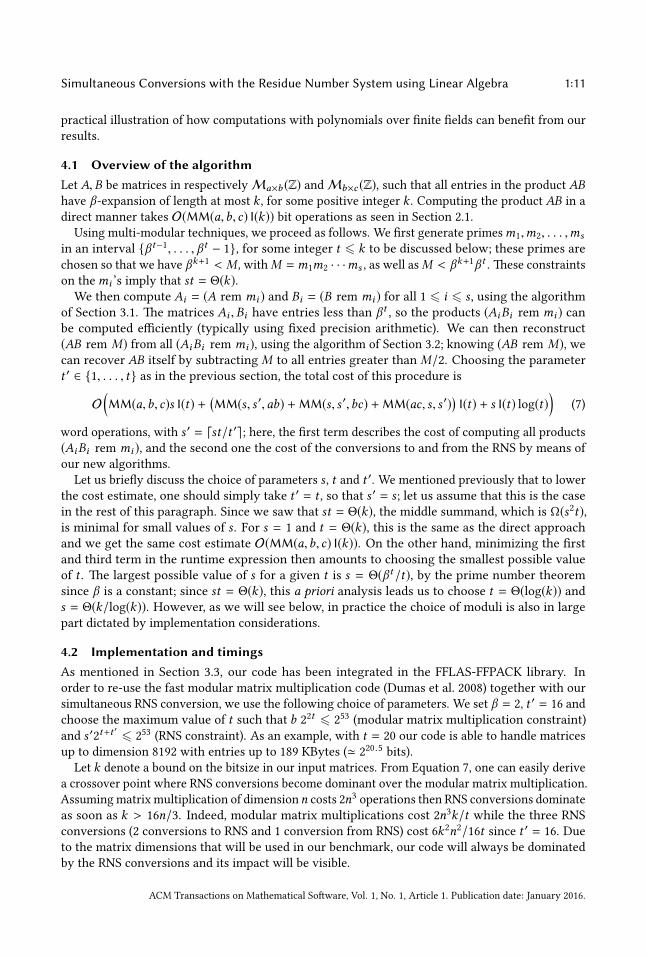
Fig. 1. Multi-precision integer matrix multiplication (time comparisons)

Our benchmarks are done on an Intel Xeon E5-2697 2.6 GHz machine and multi-threading is

not used. Figure 1 reports time of integer matrix multiplication for dierent matrix entries bitsize

(abscissa of plots) and dierent matrix dimensions (4 dierent plots). We compared our integer

matrix multiplication code in FFLAS-FFPACK with that of in FLINT (Hart 2010), and Mathemagix

(Hoeven et al. 2012) :

• FLINT provides two implementations: the direct algorithm FLINT (classic) with some

hand-tuned inline integer arithmetic, and the multi-modular algorithm FLINT (multi-modular)which uses divide-and-conquer techniques for conversions to and from the RNS. e

fmpz_mat_mul method in FLINT automatically switches between these two algorithms

based on a heuristic crossover point.

• e Algebramix package of the Mathemagix library provides three implementations: the

direct algorithm, the multi-modular one and the Kronecker+FFT algorithm. e MMX(kronecker-fft) reduces multi-precision integers to polynomials over single-precision

integers via Kronecker substitution, and then performs FFT on those polynomials (Hoeven

et al. 2016, Section 5.3). e MMX (multi-modular) plot corresponds to a hybrid multi-

modular approach that either uses quadratic or fast divide-and-conquer algorithms for

RNS conversions. e generic integer matrix multiplication code in Mathemagix switches

between these two strategies according to hardcoded thresholds.

• e FFLAS entry corresponds to our multi-modular implementations from Section 3.



For the sake of clarity, we decided to call directly the specic underlying implementations from

FLINT and Mathemagix instead of the generic code so that each plot would correspond to only one

algorithm.

From Figure 1, one can see that our method improves performance in every case for some initial

bitsize range (as our method has a super-linear complexity with respect to the bitsize, it cannot be

competitive with fast methods for large bitsize); however, when the matrix dimension increases,

the benets of our method also tend to increase. One should note that the Kronecker method with

FFT has the best asymptotic complexity in terms of integer bitsize. However, it turns out not to be

the best one when matrix dimension increases. is is conrmed in Figure 1 where for a given

bitsize value (e.g. k = 212

), MMX (kronecker-fft) implementation is the fastest code for small

matrix dimensions (e.g. n = 32) while it becomes the worst for larger ones (e.g. n = 512). Note

that the plot for matrix dimension 512 is missing a few points because some runtimes exceeded a

certain threshold.

4.3 ApplicationsWe conclude this section with an illustration of how improving matrix multiplication can impact

further, seemingly unrelated operations. Explicitly, we recall how matrix multiplication comes

into play when one deals with nite elds and how our linear algebra implementations of these

operations result in signicant speed-ups over conventional implementations for some important

operations.

Modular composition. Given a eld Fp and polynomials f ,д,h of degrees less thann over Fp , modu-

lar composition is the problem of computing f (д) mod h. No quasi-linear algorithm is known for this

task, at least in a model where one counts operations in Fp at unit cost. e best known algorithm

to date is due to Brent and Kung (Brent and Kung 1978), and is implemented in several computer

algebra systems; it allows one to perform this operations using C(n) = O(√nM(n)+MM(

√n,√n,n))

operations in Fp , where M : N→ N is such that one can multiply polynomials of degree n over Fpin M(n) operations. One should point out that there exists an almost linear algorithm in a Boolean

model due to (Kedlaya and Umans 2011), but to our knowledge no implementation of it has been

showed to be competitive with the Brent and Kung approach. Note that since the submission of

this paper, (Hoeven and Lecerf 2017) has proposed an improvement in some specic cases.

As showed in the run-time estimate, the boleneck of this algorithm is a matrix multiplication

in sizes (√n,√n) and (

√n,n), which can benet from our work. Remark that the goal is here to

multiply matrices with coecients dened modulo a potentially large p; this is done by seeing

these matrices over Z and multiplying them as such, before reducing the result modulo p.

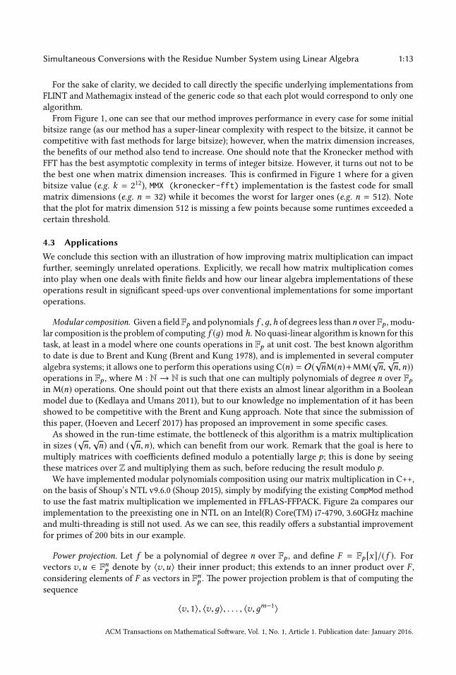
We have implemented modular polynomials composition using our matrix multiplication in C++,

on the basis of Shoup’s NTL v9.6.0 (Shoup 2015), simply by modifying the existing CompMod method

to use the fast matrix multiplication we implemented in FFLAS-FFPACK. Figure 2a compares our

implementation to the preexisting one in NTL on an Intel(R) Core(TM) i7-4790, 3.60GHz machine

and multi-threading is still not used. As we can see, this readily oers a substantial improvement

for primes of 200 bits in our example.

Power projection. Let f be a polynomial of degree n over Fp , and dene F = Fp [x]/(f ). For

vectors v,u ∈ Fnp denote by 〈v,u〉 their inner product; this extends to an inner product over F ,

considering elements of F as vectors in Fnp . e power projection problem is that of computing the

sequence

〈v, 1〉, 〈v,д〉, . . . , 〈v,дm−1〉



for a given integerm > 0, v ∈ Fnp and д in F . e best known algorithm for power projection is due

to Shoup (Shoup 1994, 1999), with a runtime that matches that of the Brent and Kung algorithm.

e dominant part of the algorithm can be formulated as a matrix multiplication similar to the one

for modular composition, this time in sizes (√n,n) and (n,

√n).

As with modular composition, we modied NTL’s ProjectPowers routine to use our matrix

multiplication implementation. Figure 2b compares our implementation to the built-in method,

and shows improvements that are very similar to the ones seen for modular composition.

0

5

10

15

20

25

30

35

40

45

10000 15000 20000 25000 30000

Tim

e in

sec

onds

Polynomial degree

NTLFFLAS

(a) Modular composition

0

5

10

15

20

25

30

35

40

45

10000 15000 20000 25000 30000

Tim

e in

sec

onds

Polynomial degree

NTLFFLAS

(b) Power projection

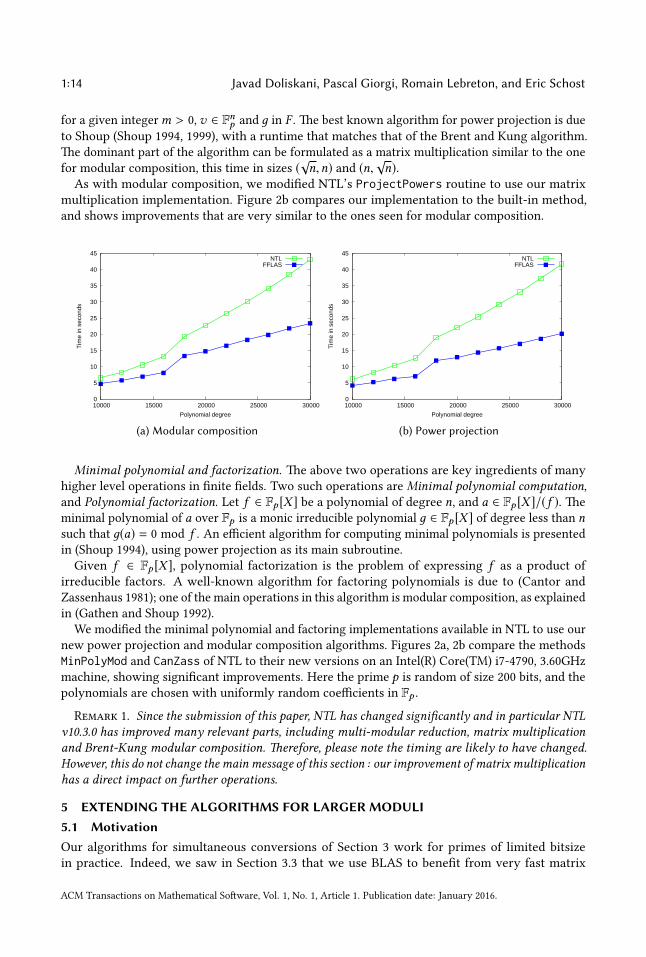
Minimal polynomial and factorization. e above two operations are key ingredients of many

higher level operations in nite elds. Two such operations are Minimal polynomial computation,

and Polynomial factorization. Let f ∈ Fp [X ] be a polynomial of degree n, and a ∈ Fp [X ]/(f ). e

minimal polynomial of a over Fp is a monic irreducible polynomial д ∈ Fp [X ] of degree less than nsuch that д(a) = 0 mod f . An ecient algorithm for computing minimal polynomials is presented

in (Shoup 1994), using power projection as its main subroutine.

Given f ∈ Fp [X ], polynomial factorization is the problem of expressing f as a product of

irreducible factors. A well-known algorithm for factoring polynomials is due to (Cantor and

Zassenhaus 1981); one of the main operations in this algorithm is modular composition, as explained

in (Gathen and Shoup 1992).

We modied the minimal polynomial and factoring implementations available in NTL to use our

new power projection and modular composition algorithms. Figures 2a, 2b compare the methods

MinPolyMod and CanZass of NTL to their new versions on an Intel(R) Core(TM) i7-4790, 3.60GHz

machine, showing signicant improvements. Here the prime p is random of size 200 bits, and the

polynomials are chosen with uniformly random coecients in Fp .

Remark 1. Since the submission of this paper, NTL has changed signicantly and in particular NTLv10.3.0 has improved many relevant parts, including multi-modular reduction, matrix multiplicationand Brent-Kung modular composition. erefore, please note the timing are likely to have changed.However, this do not change the main message of this section : our improvement of matrix multiplicationhas a direct impact on further operations.

5 EXTENDING THE ALGORITHMS FOR LARGER MODULI5.1 MotivationOur algorithms for simultaneous conversions of Section 3 work for primes of limited bitsize

in practice. Indeed, we saw in Section 3.3 that we use BLAS to benet from very fast matrix



0

10

20

30

40

50

60

70

80

10000 15000 20000 25000 30000

Tim

e in

sec

onds

Polynomial degree

NTLFFLAS

(a) Minimal polynomial computation

0

1000

2000

3000

4000

5000

6000

7000

8000

9000

10000

10000 15000 20000 25000 30000

Tim

e in

sec

onds

Polynomial degree

NTLFFLAS

(b) Polynomial factorization

multiplication and that since BLAS works on double precision oating-point numbers, it limits our

prime size to about 26 bits. ere are enough of those primes for most application of multi-modular

techniques. However, there is still an application where such a limit can be too restrictive : the

multiplication of polynomials with large integer coecients.

e multi-modular strategy is classically used to multiply such polynomials, but we need to use

particular primes. e most advantageous situation for multiplying large modular polynomials is

when one uses DFT algorithms over a ring Z/pZ which has 2d

-roots of unity, for 2d

larger than

the degree of the product. e existence of 2d

-roots of unity in Z/pZ happens if and only if 2d

divides p − 1. We call FFT primes such primes p. Historically, (Cooley and Tukey 1965) gave the

rst fast complex Fourier transform, (Gentleman and Sande 1966) used it for complex polynomial

multiplication and (Pollard 1971) adapted it for polynomial multiplication over nite elds (see

also (Gathen and Gerhard 2013, Chapter 8)).

However, the number of FFT primes is much smaller than the number of primes. Since FFT

primes are exactly primes that appear in the arithmetic progression (1 + 2dk)k ∈N, number theory

tells us that the number of FFT primes less than x is asymptotically equivalent to the numbers of

primes less than x divided by φ(2d ) = 2d−1

(where φ is Euler’s totient function).

In practice, assuming e.g. that we multiply polynomials of degree 214

and we use the bitsize limit

for the primes of Section 3 (mi < 226

), we have enough FFT primes to handle input of approximately

212.5

bits (724 Bytes), which is not sucient for some applications (for instance, in many forms of

Hensel liing algorithms, one is led to compute modulo large powers of primes).

To handle larger integer coecients with multi-modular techniques, there are at least two

directions one could take. A rst direction is to li the prime size limit of our simultaneous

RNS conversion; this requires us to provide ecient (comparable to BLAS) xed precision matrix

multiplication above 26-bits entries. e second direction is to use 3-primes FFT (Pollard 1971) (see

also (Gathen and Gerhard 2013, Chapter 8)) when we have exhausted all the possible FFT primes.

is option at least triples the asymptotic runtime per bit of the input. For the sake of completeness,

we also have to consider the direct approach, e.g. Schonhage-Strassen algorithm (Schonhage and

Strassen 1971).

In this section, we investigate the rst direction and we present a variant of our algorithm that

handles larger moduli. Note that already a slightly larger moduli will allow one to substantially

increase the possible bitsize of coecients: with our forthcoming technique, we will be able to

multiply polynomials up to degree 222

and of coecient bitsize 220

using primes of 42 bits. Note



that this is particularly interesting since FFT performances are almost not penalized when one uses

primes up to 53 bits instead of primes of 32 bits as demonstrated in (Hoeven et al. 2016).

5.2 Enlarging moduli size in practiceSince we want moduli above the BLAS limit (26-bits) but still want to perform matrix operations

using BLAS, we will cut our moduli of bitsize t into κ chunks of bitsize δ . e new parameter δrepresents the precision for which numerical matrix multiplications are feasible, i.e. s ′βδ+t

′6 2

53.

In Section 3, we considered the case where κ = 1 and δ = t . We will assume that t ′ 6 δ just as we

assumed t ′ 6 t before. Finally, we will assume that s ′ < β2δin the following sections. Indeed, this

hypothesis is veried in practice since t ′ = 16 and β = 2 implies s ′β2t ′ 6 s ′βδ+t′6 2

53 < β4t ′and

so s ′ < β2t ′ 6 β2δ.

5.3 Conversion to RNSWe start by giving the algorithm, followed by its complexity analysis. As in Section 3.1, we rst

compute all [β it ′]j = (β it′

rem mj ) for 1 6 i < s ′, 1 6 j 6 s and gather them into the matrix

B =

1 [β t ′]1 [β2t ′]1 . . . [β (s ′−1)t ′]1...

......

...

1 [β t ′]s [β2t ′]s . . . [β (s ′−1)t ′]s

∈ Ms×s ′(Z).

en we write the βδ -expansion of the matrix B as B = B0 + B1βδ + · · · + Bκ−1β

δ (κ−1)and also

compute the matrix C which gathers the β t′-expansions of the aj ’s. We rewrite Equation (4) as

(B0C)i, j + · · · + β (κ−1)δ (Bκ−1C)i, j ≡ aj (mod mi ). (8)

So, we compute the le-hand side of Equation (8) and reduce it to get aj mod mi .

Complexity estimates. e computation of [β (i+1)t ′]j from [β it ′]j is a multiplication of integers of

length 1 and κ in base βδ , which costs O(κI(δ )), just as the reduction modulomj using Equation (2).

So computing B reduces to O(ss ′κI(δ )) arithmetic operations. As before, matrices Bk and C do not

involve any arithmetic operations.

Now turning to matrix products, we get 0 6 (B`C)i, j < s ′βδ β t′< β4δ

for all `. is bound is for

theoretic purposes ; in practice all these matrix products do not exceed the BLAS limit and can

be performed eciently. In Equation (8) all the products (B`C) can be computed in one matrix

multiplication of cost O(MM(κs, s ′, r )I(δ )) by stacking vertically the B` in a matrix B ∈ Mκs×s ′(Z)and computing BC . en the sum of the (B`C) costs O(κrsδ ) and its reduction O(rsκI(δ )) using

Equation (2).

Altogether, the cost is dominated by matrix multiplication O(MM(κs, s ′, r )I(δ )), which matches

the cost in Section 3 when κ = 1. To compare with other values of κ, notice that our cost is

O(MM(s, s ′, r )I(t)) using MM(κs, s ′, r ) = O(κMM(s, s ′, r )) and the super-linearity assumption

κI(δ ) 6 I(t). So our new approach maintains the asymptotic complexity bound while liing the

restriction on the moduli size.

5.4 Conversion from RNSSimilarly, we adapt the method from Section 3.2 to our seingmi < β

t 6 βκδ . Recall that we rst

compute the pseudo-reconstructions

`i :=

s∑j=1

γi, jMj , with γi, j = (ai, juj rem mj ),uj = 1/Mj mod mj



for 1 6 j 6 s and 1 6 i 6 r , followed by a cheap reduction step ai = (ì rem M) with ì < sM .

Following the notations of Section 3.2, let G = [γi, j ] ∈ Mr×s (Z) and write U = [µ j,k ] ∈ Ms×s ′(Z)the matrix of the β t

′-expansions of all Mj . en D = [di,k ] = GU ∈ Mr×s ′(Z) satises ì =∑s ′−1

k=0di,kβ

kt ′. In our seing, the entries of G and U are respectively bounded by γi, j < mj < β

κδ,

and µ j,k < βt ′

. erefore, the entries of D are bounded by s ′βκδ+t′

which should exceed the BLAS

limit; if so we won’t be able to use BLAS to perform this product. As before, we need to expand

G = G0 +G1βδ + · · · + β (κ−1)δGκ−1 in base βδ to be able to compute D as

D = G0U + βδG1U + · · · + β (κ−1)δGκ−1U . (9)

It remains to recover ì using ì =∑s ′−1

k=0di,kβ

kt ′and reduce them modulo M .

Complexity estimates. As in Section 3.2, computingMi ,ui ,γi, j and the nal reductions (ì rem M)costs O((r + s + log(t))sI(t)). Now focusing on the linear algebra part, the products GiU have

coecients less than sβδ+t′6 s ′βδ+t

′< β4δ

; as in Section 5.3 all these products can be computed

at cost O(MM(κr , s, s ′)I(δ )) by stacking vertically the Gi . en we shi and sum these products to

recover D at cost rs ′κδ and recover the ì in the same cost.

So we get a total cost ofO(MM(κr , s, s ′)I(δ )+(r+s+log(t))sI(t))which boils down toO(MM(r , s, s ′)I(t)+sI(t) log(t)) because MM(κr , s, s ′) = O(κMM(r , s, s ′)) and κI(δ ) 6 I(t). is corresponds to the

complexity of Section 3.2. Here again, our modication for RNS conversion with larger moduli

does not change the asymptotic complexity bound while still allowing the use of BLAS.

5.5 Implementation and timingsOur modied RNS conversions have been implemented in the FFLAS-FFPACK package.

We restrict our implementation to κ = 2 as it oers a sucient range of values for integer

polynomial multiplication as mentioned in Section 5.1. As in Section 3.3, we chose β = 2 and

t ′ = 16 to simplify Kronecker substitution. e value of δ is dynamically chosen to ensure

s ′βδ+16 6 253

. Since we chose κ = 2, this means our primes must not exceed 22δ

. For small RNS

basis of bitsize less than 215

(' 4 KBytes), we can chose the maximum value δ = 26. For larger RNS

basis, we need to reduce the value of δ , e.g. with δ = 21 one can use 42-bit primes and reach an

RNS basis of 220

bits (' 131 KBytes).

Our implementation is similar to the one in Section 3.3, and we use the same tricks to improve

performance. In order to speed-up our conversions with larger primes, we always stack the matrices

to compute the κ matrix product using one larger multiplication. We have seen that the complexity

estimates of stacking are always beer because of fast matrix multiplication algorithms. And in

practice, it is oen best to have larger matrices to multiply because peak performance of BLAS is

aained starting from a certain matrix dimension. Furthermore, doubling a matrix dimension may

oer an extra level of sub-cubic matrix multiplication in FFLAS-FFPACK.

We perform our benchmark on an Intel Xeon E5-2697 2.6GHz and multi-threading is not used.

As in section 4.2, we choose the number of elements to convert from/to RNS to be 1282, and the

bitsize of integer inputs are almost twice as small as the RNS basis bitsize. In table 4, we report

the conversion time per element for a given RNS bitsize. As maer of comparison, we report the

time of our RNS conversions when κ = 1, corresponding to the ”small” prime of Section 3. We

also compare ourself to the code from FLINT library which is the fastest available contestant (see

Section 3.4) oering similar prime bitsize when κ = 2 (e.g. 59-bits).

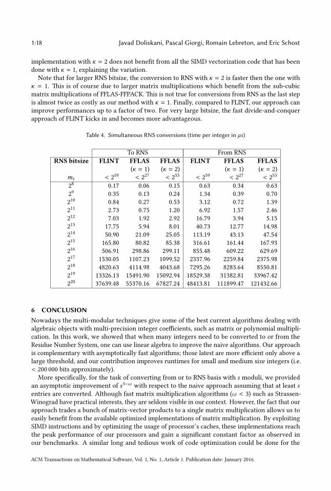
e values reported in Table 4 conrm our conclusion that the asymptotic performance numbers

should not change for dierent values of κ. However, for small RNS bitsize, one may remark slight

dierences between κ = 1 and κ = 2. For this size, the matrix multiplication is not dominant in the

complexity and the constant behind second order terms roughly double the cost. Furthermore, our



implementation with κ = 2 does not benet from all the SIMD vectorization code that has been

done with κ = 1, explaining the variation.

Note that for larger RNS bitsize, the conversion to RNS with κ = 2 is faster then the one with

κ = 1. is is of course due to larger matrix multiplications which benet from the sub-cubic

matrix multiplications of FFLAS-FFPACK. is is not true for conversions from RNS as the last step

is almost twice as costly as our method with κ = 1. Finally, compared to FLINT, our approach can

improve performances up to a factor of two. For very large bitsize, the fast divide-and-conquer

approach of FLINT kicks in and becomes more advantageous.

Table 4. Simultaneous RNS conversions (time per integer in µs)

To RNS From RNS

RNS bitsize FLINT FFLAS FFLAS FLINT FFLAS FFLAS(κ = 1) (κ = 2) (κ = 1) (κ = 2)

mi < 259 < 2

27 < 253 < 2

59 < 227 < 2

53

28

0.17 0.06 0.15 0.63 0.34 0.63

29

0.35 0.13 0.24 1.34 0.39 0.70

210

0.84 0.27 0.53 3.12 0.72 1.39

211

2.73 0.75 1.20 6.92 1.57 2.46

212

7.03 1.92 2.92 16.79 3.94 5.15

213

17.75 5.94 8.01 40.73 12.77 14.98

214

50.90 21.09 25.05 113.19 43.13 47.54

215

165.80 80.82 85.38 316.61 161.44 167.93

216

506.91 298.86 299.11 855.48 609.22 629.69

217

1530.05 1107.23 1099.52 2337.96 2259.84 2375.98

218

4820.63 4114.98 4043.68 7295.26 8283.64 8550.81

219

13326.13 15491.90 15092.94 18529.38 31382.81 33967.42

220

37639.48 55370.16 67827.24 48413.81 111899.47 121432.66

6 CONCLUSIONNowadays the multi-modular techniques give some of the best current algorithms dealing with

algebraic objects with multi-precision integer coecients, such as matrix or polynomial multipli-

cation. In this work, we showed that when many integers need to be converted to or from the

Residue Number System, one can use linear algebra to improve the naive algorithms. Our approach

is complementary with asymptotically fast algorithms; those latest are more ecient only above a

large threshold, and our contribution improves runtimes for small and medium size integers (i.e.

< 200 000 bits approximately).

More specically, for the task of converting from or to RNS basis with s moduli, we provided

an asymptotic improvement of s3−ωwith respect to the naive approach assuming that at least s

entries are converted. Although fast matrix multiplication algorithms (ω < 3) such as Strassen-

Winograd have practical interests, they are seldom visible in our context. However, the fact that our

approach trades a bunch of matrix-vector products to a single matrix multiplication allows us to

easily benet from the available optimized implementations of matrix multiplication. By exploiting

SIMD instructions and by optimizing the usage of processor’s caches, these implementations reach

the peak performance of our processors and gain a signicant constant factor as observed in

our benchmarks. A similar long and tedious work of code optimization could be done for the



naive algorithms, but we can reasonably doubt that we would reach the same peak performance,

in particular because of the sequential nature of this approach. Finally, even if our gain is only

constant, its impact is substantial because it applies to many important issues, e.g. integer matrix

multiplication, polynomial factorization or minimal polynomial computation.

In some specic cases, the prime bitsize limitation of the implementation of Section 3 is a problem

because we lack primes when handling larger integer, all the moreso if we need specic primes

(e.g. Fourier primes). In these laer cases, we showed by spliing the moduli into several parts that

we are still able to reduce the computation to matrix multiplication with small entries and obtain

the same complexity and performances as for small moduli.

Our perspectives are to further improve our approach and future work should investigate at

least two directions. First, when integer entries are very large, one can use a combination of the

divide-and-conquer strategy to reduce entries below a certain bound and of our approach to nalize

the conversions. is hybrid technique must ensure beer performances in practice for a wider

range of integer bitsizes. Second, when dealing with moduli exceeding the limit of Section 3.3,

one could want to enlarge the value of t ′ (the size of the digits in the Kronecker substitution) to

be as large as t (the size of the moduli). Indeed, t = t ′ was the best choice of parameters for the

complexity analyses of Section 3 and Section 5 could not allow this. ere, we are given to perform

a matrix multiplication of entries of size κδ . Such integer matrices can be viewed as polynomial

matrices over Z[X ] of degree κ with coecients of size δ (i.e. βδ is replaced by the indeterminate

X ). Hence, one can use any subquadratic polynomial multiplication schemes to perform such

multiplication over Z[X ] and evaluate the result at X = βδ . Of course, one need to be careful in the

denition of the value of δ to guarantee that no overow occurs, but we are condent that this

laer approach should provide further improvement.

ACKNOWLEDGMENTSWe are grateful to the anonymous referees for their thorough reading and helpful comments. is

work has been supported by the French ANR under the grants HPAC (ANR-11-BS02-013), CATREL

(ANR-12-BS02-001), NSERC and the Canada Research Chairs program.

REFERENCESA. V. Aho, J. E. Hopcro, and J. D. Ullman. 1974. e Design and Analysis of Computer Algorithms. Addison-Wesley.

P. Barre. 1986. Implementing the Rivest Shamir and Adleman public key encryption algorithm on a standard digital signal

processor. In Advances in Cryptology, CRYPTO’86 (LNCS), Vol. 263. Springer, 311–326.

D. J. Bernstein. 2004. Scaled remainder trees. hps:// cr.yp.to/arith/ scaledmod-20040820.pdf 18 (2004).

A. Borodin and R. Moenck. 1974. Fast modular transforms. J. Comput. System Sci. 8, 3 (1974), 366–386.

W. Bosma, J. Cannon, and C. Playoust. 1997. e Magma algebra system. I. The user language. J. Symbolic Comput. 24, 3-4

(1997), 235–265. hps://doi.org/10.1006/jsco.1996.0125 Computational algebra and number theory (London, 1993).

R. P. Brent and H. T. Kung. 1978. Fast algorithms for manipulating formal power series. Journal of the Association forComputing Machinery 25, 4 (1978), 581–595.

R. P. Brent and P. Zimmermann. 2010. Modern Computer Arithmetic. Cambridge University Press, New York, NY, USA.

D. G. Cantor and H. Zassenhaus. 1981. A new algorithm for factoring polynomials over nite elds. Math. Comp. (1981),

587–592.

S. Cook. 1966. On the minimum computation time of functions. Ph.D. Dissertation. Harvard University.

J. W. Cooley and J. W. Tukey. 1965. An Algorithm for the Machine Calculation of Complex Fourier Series. Math. Comp. 19,

90 (1965), 297–301. hps://doi.org/10.2307/2003354

D. Coppersmith and S. Winograd. 1990. Matrix multiplication via arithmetic progressions. J. Symb. Comp 9, 3 (1990),

251–280.

J.-G. Dumas, T. Gautier, M. Giesbrecht, P. Giorgi, B. Hovinen, E. Kaltofen, B. D. Saunders, W. J. Turner, G. Villard, et al.

2002. LinBox: A generic library for exact linear algebra. In Proceedings of the 2002 International Congress of MathematicalSoware, Beijing, China. World Scientic Pub, 40–50.


https://cr.yp.to/arith/scaledmod-20040820.pdf

https://doi.org/10.1006/jsco.1996.0125

https://doi.org/10.2307/2003354


J.-G. Dumas, P. Giorgi, and C. Pernet. 2008. Dense Linear Algebra over Word-Size Prime Fields: the FFLAS and FFPACK

Packages. ACM Trans. on Mathematical Soware (TOMS) 35, 3 (2008), 1–42. hps://doi.org/10.1145/1391989.1391992

FFLAS-FFPACK-Team. 2016. FFLAS-FFPACK: Finite Field Linear Algebra Subroutines / Package (v2.2.2 ed.). hp://github.com/

linbox-team/as-pack.

M. Frigo and S. G. Johnson. 2005. e design and implementation of FFTW3. Proc. IEEE 93, 2 (2005), 216–231. Special issue

on “Program Generation, Optimization, and Platform Adaptation”.

M. Furer. 2007. Faster integer multiplication. In STOC’07. ACM, 57–66.

J. von zur Gathen and J. Gerhard. 2013. Modern Computer Algebra (3 ed.). Cambridge University Press, New York, NY, USA.

J. von zur Gathen and V. Shoup. 1992. Computing Frobenius maps and factoring polynomials. Computational complexity 2,

3 (1992), 187–224.

W. M. Gentleman and G. Sande. 1966. Fast Fourier Transforms: For Fun and Prot. In Proceedings of the November 7-10, 1966,Fall Joint Computer Conference (AFIPS ’66 (Fall)). ACM, New York, NY, USA, 563–578. hps://doi.org/10.1145/1464291.

1464352

P. Giorgi, L. Imbert, and T. Izard. 2013. Parallel modular multiplication on multi-core processors. In 21st IEEE Symposium onComputer Arithmetic (ARITH). 135–142. hps://doi.org/10.1109/ARITH.2013.20

GMP-Team. 2015. Multiple precision arithmetic library. (2015). hps://gmplib.org/.

K. Goto and R. van de Geijn. 2008. High-performance implementation of the level-3 BLAS. ACM Trans. Math. Soware 35, 1

(2008), 4.

T. Hagerup. 1998. Sorting and Searching on the Word RAM. In Proceedings of the 15th Annual Symposium on eoreticalAspects of Computer Science (STACS ’98). Springer-Verlag, 366–398. hp://dl.acm.org/citation.cfm?id=646513.695510

W. B. Hart. 2010. Fast library for number theory: an introduction. In Mathematical Soware–ICMS 2010. Springer, 88–91.

hp://www.intlib.org/.

D. Harvey and J. van der Hoeven. 2014. On the complexity of integer matrix multiplication. Technical Report. HAL.

hp://hal.archives-ouvertes.fr/hal-01071191.

D. Harvey, J. van der Hoeven, and G. Lecerf. 2016. Even faster integer multiplication. Journal of Complexity 36 (2016), 1 –

30. hps://doi.org/10.1016/j.jco.2016.03.001

J. van der Hoeven. 2016. Faster Chinese remaindering. Technical Report. HAL. hp://hal.archives-ouvertes.fr/hal-01403810.

J. van der Hoeven and G. Lecerf. 2017. Modular composition via factorization. Technical Report. HAL. hp://hal.

archives-ouvertes.fr/hal-01457074.

J. van der Hoeven, G. Lecerf, B. Mourrain, P. Trebuchet, J. Berthomieu, D. N. Diaa, and A. Mantzaaris. 2012. Mathemagix:

the quest of modularity and eciency for symbolic and certied numeric computation? ACM Communications inComputer Algebra 45, 3/4 (2012), 186–188. hp://www.mathemagix.org/.

J. van der Hoeven, G. Lecerf, and G. intin. 2016. Modular SIMD Arithmetic in Mathemagix. ACM Trans. Math. Sow. 43,

1 (Aug. 2016), 5:1–5:37. hps://doi.org/10.1145/2876503

MKL Intel. 2007. Intel math kernel library. (2007).

K. S. Kedlaya and C. Umans. 2011. Fast Polynomial Factorization and Modular Composition. SIAM J. Computing 40, 6 (2011),

1767–1802.

F. Le Gall. 2014. Powers of Tensors and Fast Matrix Multiplication. In Proceedings of the 39th International Symposium onSymbolic and Algebraic Computation (ISSAC ’14). ACM, New York, NY, USA, 296–303. hps://doi.org/10.1145/2608628.

2608664

LinBox-Team. 2016. LinBox: C++ library for exact, high-performance linear algebra (v1.4.2 ed.). hp://github.com/linbox-team/

linbox.

C. Pernet. 2015. Exact Linear Algebra Algorithmic: eory and Practice. In Proceedings of the 2015 ACM on InternationalSymposium on Symbolic and Algebraic Computation (ISSAC ’15). ACM, New York, NY, USA, 17–18. hps://doi.org/10.

1145/2755996.2756684

J. M. Pollard. 1971. e fast Fourier transform in a nite eld. Math. Comp. 25, 114 (1971), 365–374. hps://doi.org/10.1090/

S0025-5718-1971-0301966-0

M. Puschel, J. M. F. Moura, J. Johnson, D. Padua, M. Veloso, B. Singer, J. Xiong, F. Franchei, A. Gacic, Y. Voronenko, K.

Chen, R. W. Johnson, and N. Rizzolo. 2005. SPIRAL: code generation for DSP transforms. Proceedings of the IEEE, specialissue on “Program Generation, Optimization, and Adaptation” 93, 2 (2005), 232– 275.

A. Schonhage and V. Strassen. 1971. Schnelle Multiplikation großer Zahlen. Computing 7 (1971), 281–292.

V. Shoup. 1994. Fast construction of irreducible polynomials over nite elds. Journal of Symbolic Computation 17, 5 (1994),

371–391.

V. Shoup. 1995. A new polynomial factorization algorithm and its implementation. Journal of Symbolic Computation 20, 4

(1995), 363–397.

V. Shoup. 1999. Ecient computation of minimal polynomials in algebraic extensions of nite elds. In ISSAC’99. ACM,

53–58.


https://doi.org/10.1145/1391989.1391992

http://github.com/linbox-team/fflas-ffpack

http://github.com/linbox-team/fflas-ffpack

https://doi.org/10.1145/1464291.1464352

https://doi.org/10.1145/1464291.1464352

https://doi.org/10.1109/ARITH.2013.20

https://gmplib.org/

http://dl.acm.org/citation.cfm?id=646513.695510

http://www.flintlib.org/

http://hal.archives-ouvertes.fr/hal-01071191

https://doi.org/10.1016/j.jco.2016.03.001




http://www.mathemagix.org/

https://doi.org/10.1145/2876503

https://doi.org/10.1145/2608628.2608664

https://doi.org/10.1145/2608628.2608664

http://github.com/linbox-team/linbox

http://github.com/linbox-team/linbox

https://doi.org/10.1145/2755996.2756684

https://doi.org/10.1145/2755996.2756684

https://doi.org/10.1090/S0025-5718-1971-0301966-0

https://doi.org/10.1090/S0025-5718-1971-0301966-0


V. Shoup. 2015. NTL: A library for doing number theory. (2015). Version 9.6.0, hp://www.shoup.net/ntl/.

A. Stothers. 2010. On the Complexity of Matrix Multiplication. Ph.D. Dissertation. University of Edinburgh.

V. Strassen. 1969. Gaussian elimination is not optimal. Numer. Math. 13, 4 (1969), 354–356. hps://doi.org/10.1007/BF02165411

V. Vassilevska Williams. 2012. Multiplying Matrices Faster an Coppersmith-winograd. In Proceedings of the Forty-fourthAnnual ACM Symposium on eory of Computing (STOC ’12). ACM, New York, NY, USA, 887–898. hps://doi.org/10.

1145/2213977.2214056

R. C. Whaley, A. Petitet, and J. J. Dongarra. 2001. Automated empirical optimizations of soware and the ATLAS project.

Parallel Comput. 27, 1 (2001), 3–35.


http://www.shoup.net/ntl/

https://doi.org/10.1007/BF02165411

https://doi.org/10.1145/2213977.2214056

https://doi.org/10.1145/2213977.2214056

simultaneous conversions with the residue number system ...lebreton/fichiers/doliskani, giorgi,...

Documents