simulink simulation of proportional navigation and · pdf filenaval postgraduate school...
TRANSCRIPT
Calhoun: The NPS Institutional Archive
Theses and Dissertations Thesis Collection
1995-03
Simulink simulation of proportional navigation and
command to line of sight missile guidance
Costello, Patrick.
Monterey, California. Naval Postgraduate School
http://hdl.handle.net/10945/31532

NAVAL POSTGRADUATE SCHOOL MONTEREY, CALIFORNIA
I t- I
THESIS
SIMULINK SIMULATION OF PROPORTIONAL I NAVIGATION AND COMMAND TO LINE OF SIGHT MISSILE GUIDANCE
bY
Patrick Costello
March, 1995
I ThesisAdvisor: Harold A. Titus
Approved for public release; distribution is unlimited.
19950125 092
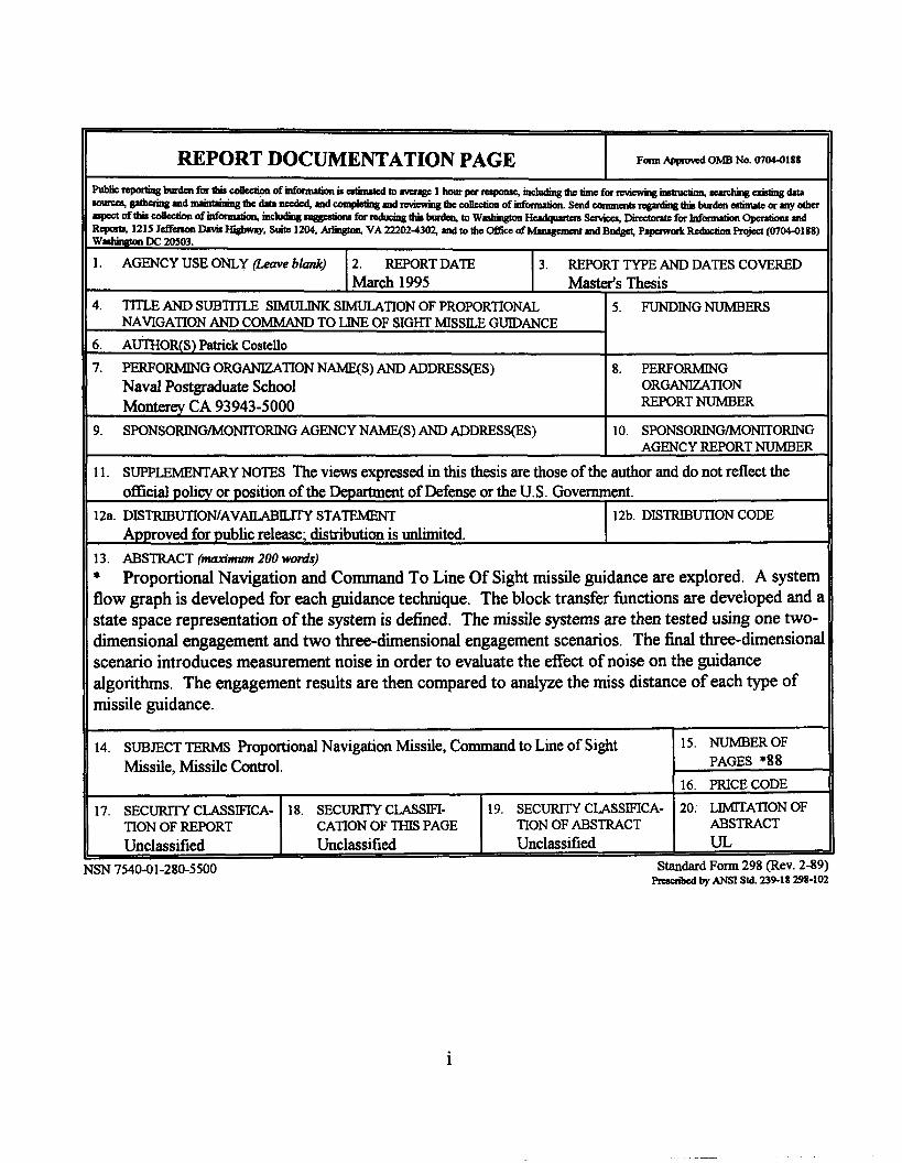
REPORT DOCUMENTATION PAGE
15. NUMBEROF 14. SUBJECT TERMS Proportional Navigation Missile, Command to Line of Sight Missile, Missile Control. PAGES *88
16. PRICECODE
17. S E C W CLASSIFICA- 18. SECURITY CLASSIFI- 19. SECURITY CLASSIFICA- 20. LIMlTATION OF TION OF REPORT CATION OF THIS PAGE TION OF ABSTRACT ABSTRACT Unclassified Unclassified Unclassified UL
J
It Form Approved OMB No. 0704-0188 I
1

ii

Approved for public release; distribution is unlimited.
---&I
Accesioii Fdr NTIS C K A t l u U I I 4 I 1 o :I i 1 ce d -1
J i i s L i f I ca ? i o ri
orlc TAB 0 - ......__. .....................
_I---
BY . ........ *.-_ --.--'
Dish ibtltion I ----
Availabil ity Codes .---.-
SIMULINK SIMULATION OF PROPORTIONAL NAVIGATION AND COMMAND TO LINE OF SIGHT MISSILE GUIDANCE
Patrick Costello Lieutenant, United States Navy
B.S.E.E, Marquette University, 1987
Submitted in partial fulfillment of the requirements for the degree of
MASTER OF SCIENCE ELECTRICAL ENGINEERING
from the
NAVAL POSTGRADUATE SCHOOL March 1995
Author:
Approved by:
R. G. Hutkfhns, Second Reader
Y -fsv Michael A. Morgan, Chairman Department of Electrical and Computer Engineering
iii
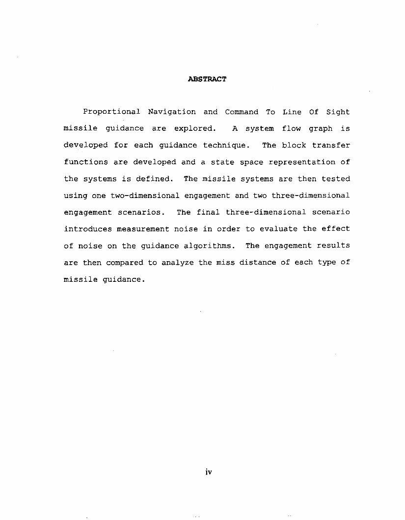
ABSTRACT
Proportional Navigation and Command To Line Of Sight
missile guidance are explored. A system flow graph is
developed for each guidance technique. The block transfer
functions are developed and a state space representation of
the systems is defined. The missile systems are then tested
using one two-dimensional engagement and two three-dimensional
engagement scenarios. The final three-dimensional scenario
introduces measurement noise in order to evaluate the effect
of noise on the guidance algorithms. The engagement results
are then compared to analyze the miss distance of each type of
missile guidance.
iV
TABLE OF CONTENTS
I . INTRODUCTION . . . . . . . . . . . . . . . . . . . . 1
I1 . MISSILE GUIDANCE LAWS . . . . . . . . . . . . . . . 3
A . GENERAL . . . . . . . . . . . . . . . . . . . . 3
B . PROPORTIONAL NAVIGATION . . . . . . . . . . . . 4 C . COMMAND GUIDANCE . . . . . . . . . . . . . . . . 6
I11 . SYSTEM DEVELOPMENT . . . . . . . A . OVERVIEW . . . . . . . . . . . B . RADAR DEVELOPMENT . . . . . .
1 . Proportional Navigation . 2 . Command Guidance . . . .
C . SEEKER DEVELOPMENT . . . . . . 1 . Proportional Navigation . 2 . Command Guidance . . . .
D . GUIDANCE DEVELOPMENT . . . . . 1 . Proportional Navigation . 2 . Command Guidance . . . .
E . AUTOPILOT DEVELOPMENT . . . . 1 . Proportional Navigation . 2 . Command Guidance . . . .
F . MISSILE AND TARGET KINEMATICS G . KALMAN FILTER DEVELOPMENT . .
. . . . . . . . . 7
. . . . . . . . . 7
. . . . . . . . . 7
. . . . . . . . . 7
. . . . . . . . . 9
. . . . . . . . . 10
. . . . . . . . . 13
. . . . . . . . . 13
. . . . . . . . . 13
. . . . . . . . . 13
. . . . . . . . . 15
. . . . . . . . . 15
. . . . . . . . . i a
. . . . . . . . . 1 9
. . . . . . . . . 20
. . . . . . . . . . . . . . . . . . . . . . . . . . . . . . . . . . . . .
IV . SIMULATION RESULTS 25
A . OVERVIEW 25
B . SIMULATION ASSUMPTIONS 25
C . SIMULATION SCENARIOS 26
. . . . . . . . . . . . . . . . . . . . . . . . . . .
1 . Constant Velocity In Two Dimensions . . . . 26 2 . Constant Velocity In Three Dimensions . . . 26
V
3 . Three-Dimensional Simulation With Radar Noise . . . . . . . . . . . . . . . . . . . . . 27
D . RESULTS AND SIMULATION COMPARISON . . . . . . . 27
V . CONCLUSIONS AND RECOMMENDATIONS . . . . . . . . . . . 33 A . CONCLUSIONS . . . . . . . . . . . . . . . . . . 33 B . RECOMMENDATIONS . . . . . . . . . . . . . . . . 33
APPENDIX . . . . . . . . . . . . . . . . . . . . . . . . 35
A . COMMAND GUIDED MISSILE PLOTS FOR SCENARIO 1 . . 35 B . PROPORTIONAL NAVIGATION MISSILE PLOTS FOR SCENARIO 2
. . . . . . . . . . . . . . . . . . . . . . . 40
C . COMMAND GUIDED MISSILE PLOTS FOR SCENARIO 2 . . 47
D . PROPORTIONAL NAVIGATION MISSILE PLOTS FOR SCENARIO 3 . . . . . . . . . . . . . . . . . . . . . . . 55
E . COMMAND GUIDED MISSILE PLOTS FOR SCENARIO 3 . . 59
F . PROPORTIONAL NAVIGATION SIMULINK MODEL . . a . . 62
G . COMMAND GUIDANCE SIMULINK MODEL . . . . . . . . 6 8
H . MISCELLANEOUS MATLAB CODE . . . . . . . . . . . . 7 6
BIBLIOGRAPHY . . . . . . . . . . . . . . . . . . . . . . 7 9
INITIAL DISTRIBUTION LIST . . . . . . . . . . . . . . . . 81
I. INTRODUCTION
A guided missile can be controlled using two different methods. The first is when the missile contains its own guidance system. This type of missile is beneficial in that once fired it will track its target. The second type of guidance has a ground fire control system to command the missile. This type of missile, called command guided, does not contain a target seeker. Two radars, or one radar capable of tracking two targets, are required at the fire control station; one will track the missile and the other the target. The fire control system will calculate the required missile acceleration commands and relay them to the missile by either a radio link or fiber optic cable.
The type of guidance system implemented is largely dependent on the missile's mission. A long range missile will
need a self contained guidance system. A point defense missile will use a self contained seeker or command guidance.
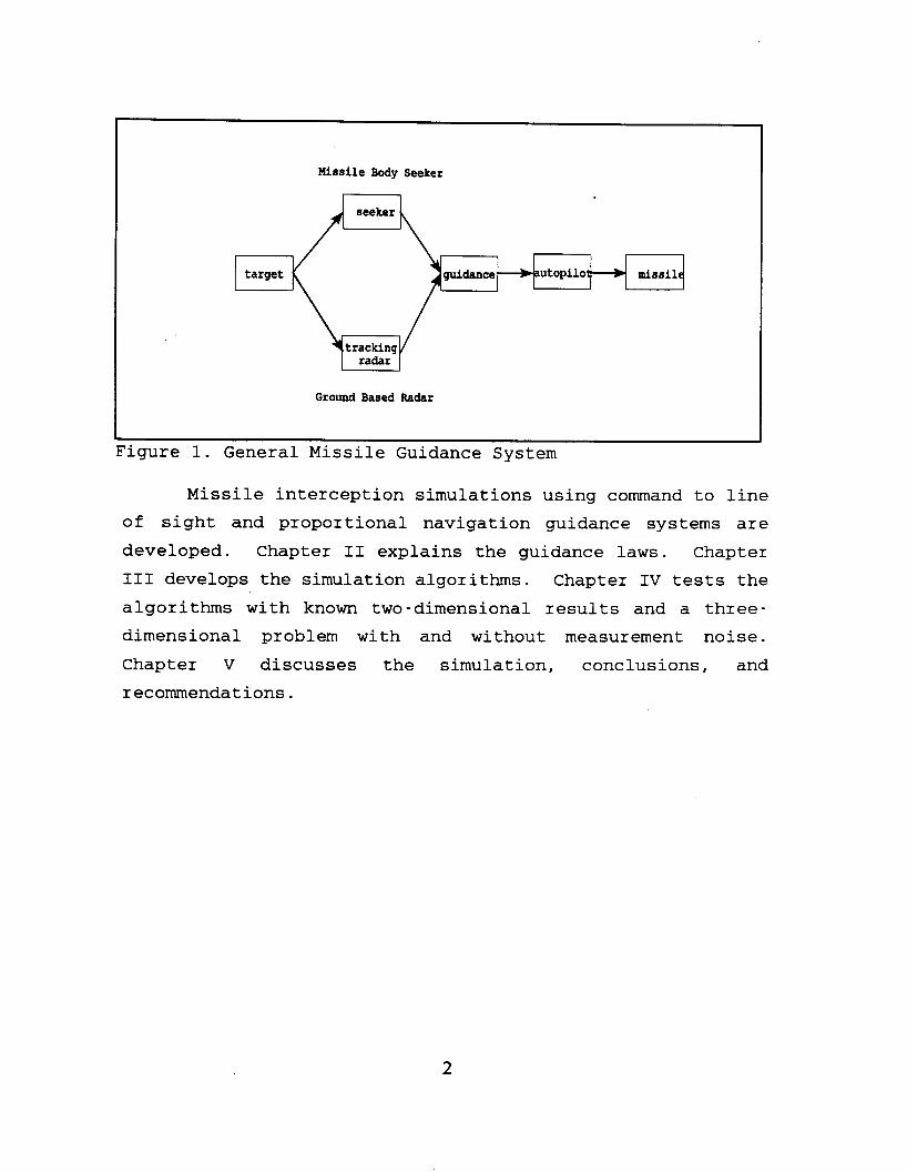
The guidance system supplies the input to the missile control system. We will use a r o l l stabilized "skid- to- turn" missile. The roll stabilization will permit a simpler analysis because there is no coupling between pitch and yaw. Figure 1 shows a block diagram for a missile control system.
1
Missile Body Seeker
seeker
missil guidance utopilo target
tracking radar
Ground Based Radar
Figure 1. General Missile Guidance System
Missile interception simulations using command to line of sight and proportional navigation guidance systems are developed. Chapter I1 explains the guidance laws. Chapter I11 develops the simulation algorithms. Chapter IV tests the algorithms with known two-dimensional results and a three- dimensional problem with and without measurement noise. Chapter V discusses the simulation, conclusions, and recommendations.
2
11. MISSILE GUIDANCE LAWS
A. GWERAL
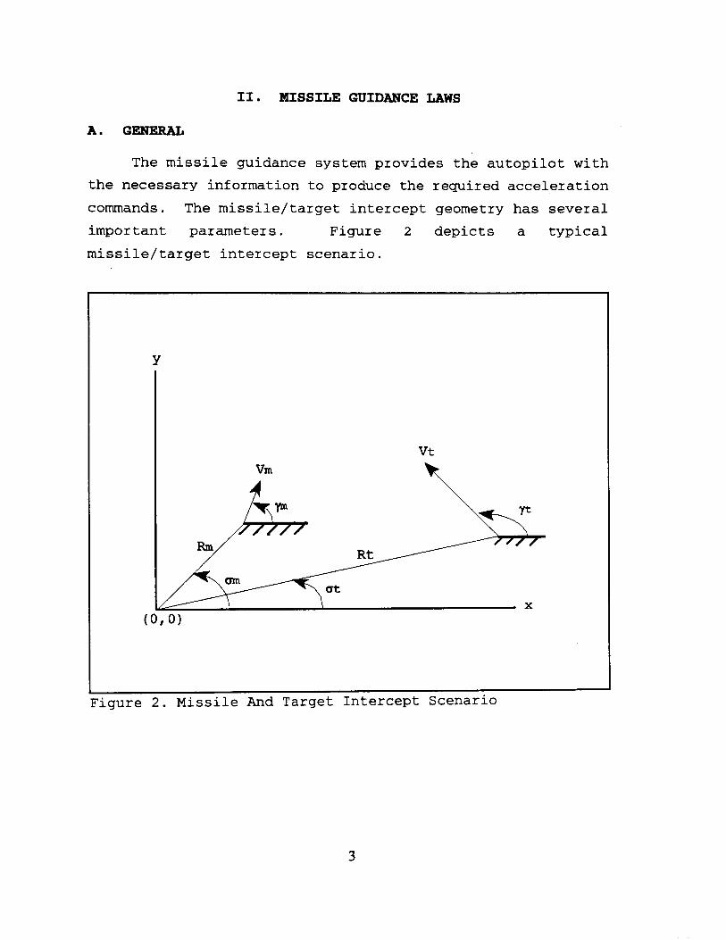
The missile guidance system provides the autopilot with the necessary information to produce the required acceleration commands. The missile/target intercept geometry has several important parameters. Figure 2 depicts a typical missile/target intercept scenario.
Y
Vt
\ Vm
X
Figure 2. Missile And Target Intercept Scenario
3
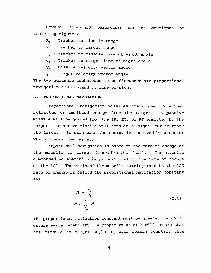
Several important parameters can be developed by analyzing Figure 2.
: Tracker to missile range
R, : Tracker to target range om : Tracker to missile line-of-sight angle ot : Tracker to target line-of-sight angle ym : Missile velocity vector angle yt : Target velocity vector angle
The two guidance techniques to be discussed are proportional navigation and command-to-line-of-sight.
B. PROPORTIONAL NAVIGATION
Proportional navigation missiles are guided by either reflected or emmitted energy from the target. A passive missile will be guided from the IR, EO, or RF emmitted by the target. An active missile will send an RF signal out to track the target. In each case the energy is received by a seeker which tracks the target.
Proportional navigation is based on the rate of change of the missile to target line-of -sight (LOS) . The missile commanded acceleration is proportional to the rate of change of the LOS. The ratio of the missile turning rate to the LOS
rate of change is called the proportional navigation constant
(N) .
V N = 2 N'
V m
(2 1)
The proportional navigation constant must be greater than 2 to ensure system stability. A proper value of N will ensure that
the missile to target angle om, will remain constant thus
4
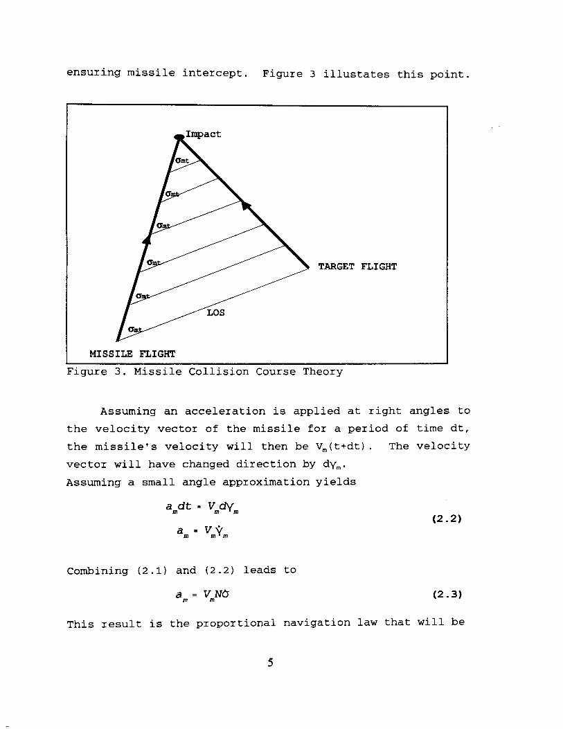
ensuring missile intercept. Figure 3 illustates this point.
TARGET F L I G H T
1 MISSILE E'LIGHT
Figure 3 . Missile Collision Course Theory
Assuming an acceleration is applied at right angles to the velocity vector of the missile for a period of time dt, the missile's velocity will then be V,(t+dt). The velocity vector will have changed direction by dy,. Assuming a small angle approximation yields
amdt = Vmdym
am = vmvm
Combining (2.1) and ( 2 . 2 ) leads to
am = V NO m
This result is the proportional navigation law that will be
5
implemented in this simulation.
C . COMMAND GUIDANCE
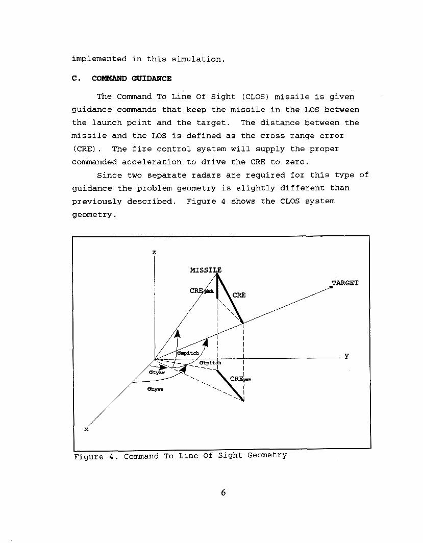
The Command To Line Of Sight (CLOS) missile is given guidance commands that keep the missile in the LOS between the launch point and the target. The distance between the missile and the LOS is defined as the cross range error ( C R E ) .
commanded acceleration to drive the CRE to zero. The fire control system will supply the proper
Since two separate radars are required for this type of guidance the problem geometry is slightly different than previously described. Figure 4 shows the CLOS system geometry.
X'
Figure 4. Command To Line Of Sight Geometry
6
111. SYSTEM DEVELOPMENT
A. OVERVIEW
The system block diagram is shown in Figure 1. The block transfer functions, system dynamics, and simulation equations will be developed for the simulation.
B. RADAR DEVELOPMWT
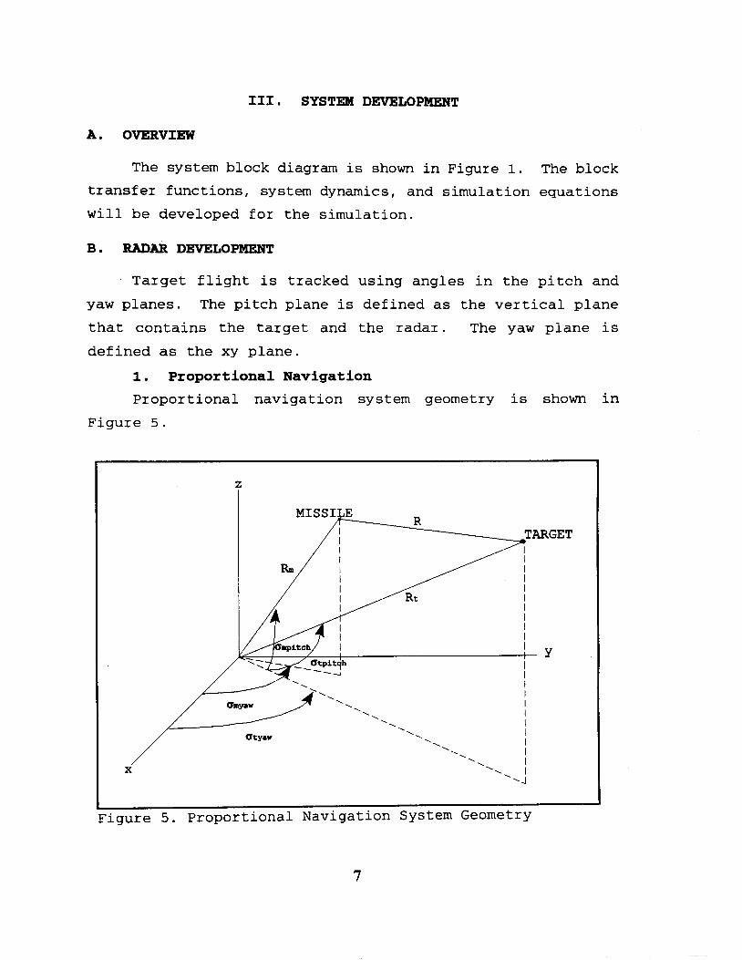
Target flight is tracked using angles in the pitch and yaw planes. The pitch plane is defined as the vertical plane that contains the target and the radar. The yaw plane defined as the xy plane.
1. Proportional Navigation Proportional navigation system geometry is shown
Figure 5 .
is
in
I I I I
I I I I I I I I I I I
‘.I
[ Y
. . ‘ . . . . . . . .. . . . . . atysv
X
Figure 5. Proportional Navigation System Geometry
7
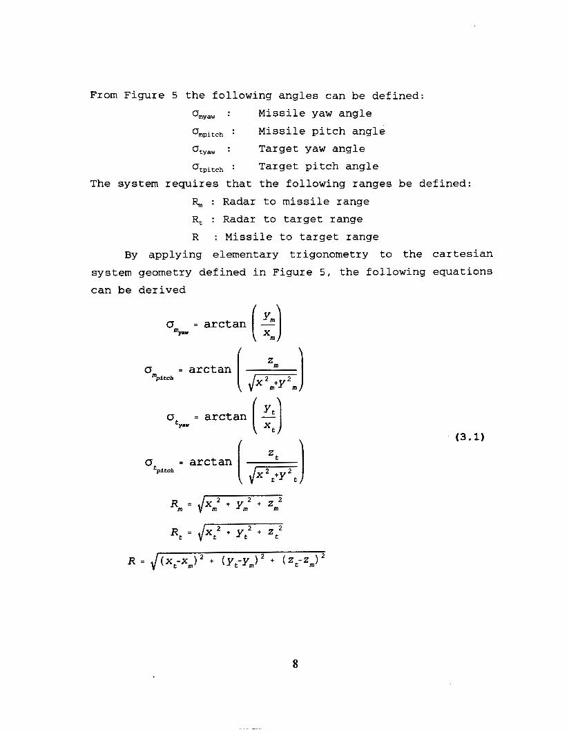
From Figure 5 the following angles can be defined: %yaw : Missile yaw angle Ompitch : Missile pitch angle Otyaw : Target yaw angle Otpitch * * Target pitch angle
The system requires that the following ranges be defined: % : Radar to missile range Rt : Radar to target range R : Missile to target range
By applying elementary trigonometry to the Cartesian system geometry defined in Figure 5, the following equations can be derived
o tY.W = arctan [ 21 (3.1)
8

The radar system will produce the following angles
%w : Missile to target yaw plane angle Opitch : Missile to target pitch plane angle
The angles are given by the equations
The radar will send these angles to the respective yaw and pitch seeker elements.
2 . Command Guidance The CLOS radar will produce a cross range error signal
and relay this signal to the missile autopilot. The cross range error is the distance between the missile and the radar to target LOS. Figure 4 shows the CLOS geometry.
From Figure 4 and vector calculus the cross range error of the missile can be defined as follows
This calculation yields the following equation
The missile autopilot requires that the cross range error be broken into the yaw and pitch components. Analyzing Figure 4 yields the following equations
9
z--
CRE = J- s i g n ( 0 - o ) tpftdr %itch p i t c h
(3.5)
The sign function ensures that the pitch plane cross range error can be positive or negative. A positive cross range error indicates that the missile is leading the LOS. A
negative cross range error indicates the missile is trailing the LOS.
C . SEEKER DEVELOPMENT
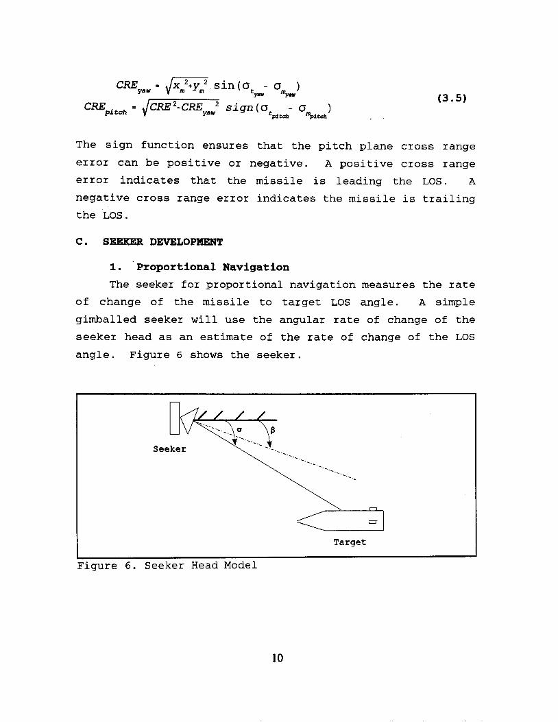
1. Proportional Navigation The seeker fo r proportional navigation measures the rate
of change of the missile to target LOS angle. A simple gimballed seeker will use the angular rate of change of the seeker head as an estimate of the rate of change of the LOS
angle. Figure 6 shows the seeker.
n
I Target
Figure 6. Seeker Head Model
10
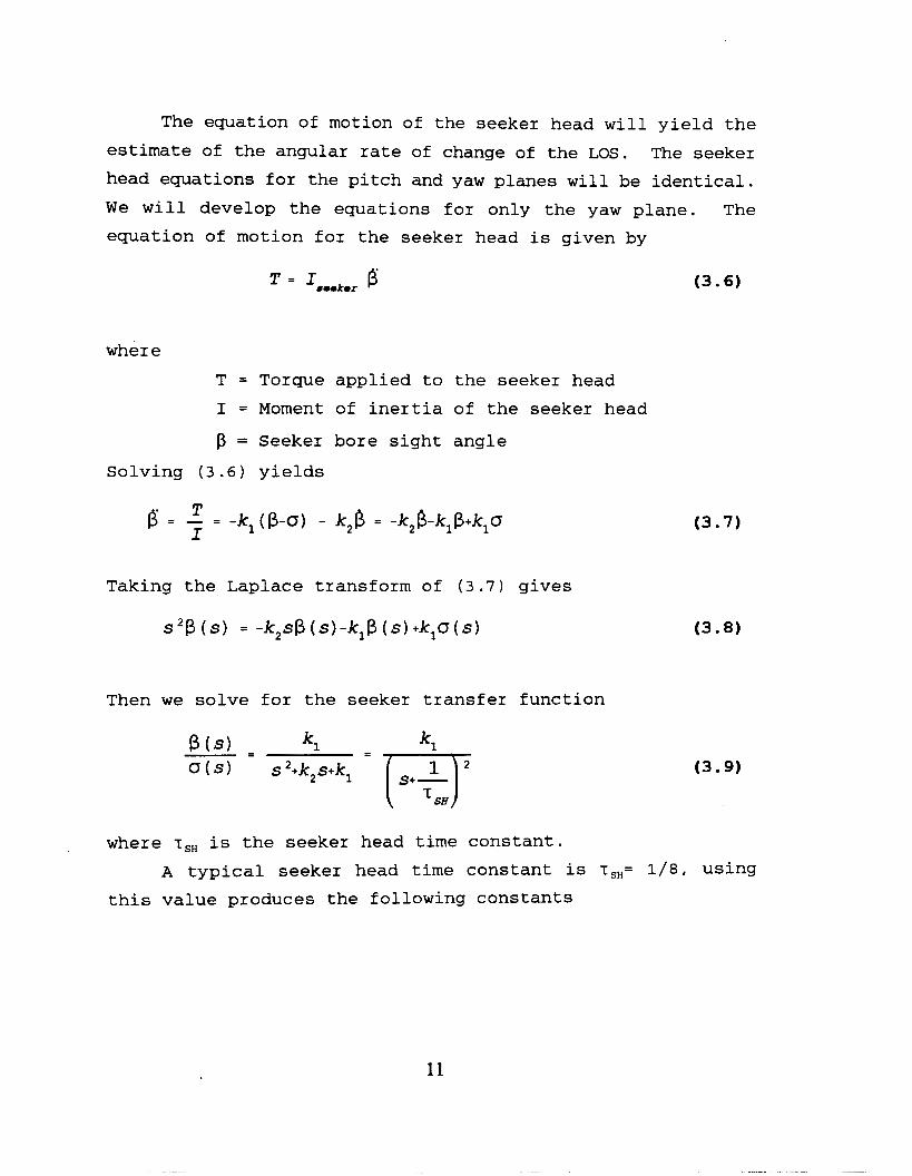
The equation of motion of the seeker head will yield the estimate of the angular rate of change of the LOS. The seeker head equations for the pitch and yaw planes will be identical. We will develop the equations for only the yaw plane. The equation of motion for the seeker head is given by
= Iseekcr Is’
where T = Torque applied to the seeker head I = Moment of inertia of the seeker head
p = Seeker bore sight angle
Solving ( 3 . 6 ) yields
* T I
13 = - = -k, ( p-0) - k2P = -k ,~ -k ,p+kp
Taking the Laplace transform of (3.7) gives
s 2 p ( s ) = -k2sp(s)-k,p(s)+k,0(S)
(3.7)
Then we solve for the seeker transfer function
P ( s ) kl kl - =
(3 9)
where T~~ is the seeker head time constant. A typical seeker head time constant is T ~ ~ = 1/8, using
this value produces the following constants
11
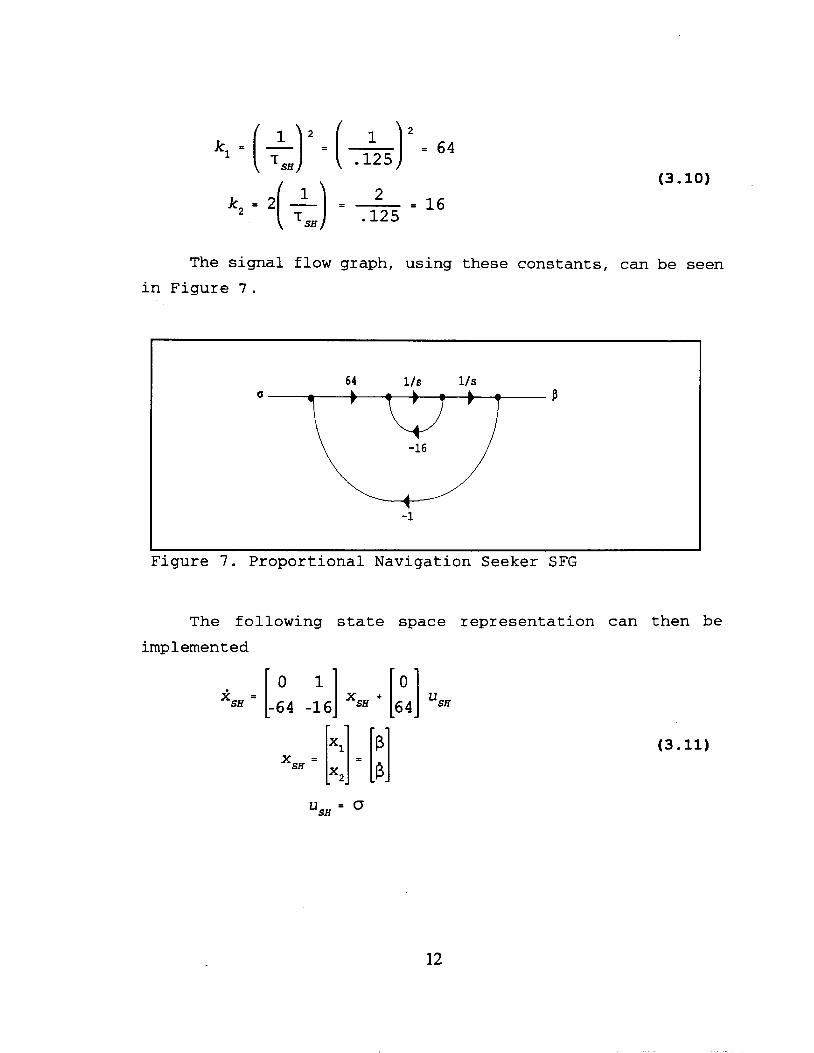
k, = ($)* = [ = 64
* 16 (3.10)
The signal flow graph, using these constants, can be seen in Figure 7.
\ \ -16 /
v -1
Figure 7. Proportional Navigation Seeker SFG
The following state space representation can then be implemented
(3.11)
12

2. Command Guidance The CLOS missile control system does not contain a seeker
head. All missile control functions are processed and developed by the fire control system located at the radar site.
D. GUIDANCE DEVELOPMEXT
1. Proportional Navigation The missile guidance system implements the proportional
navigation law explained in Chapter 11. The major difference is that an estimate of the angular LOS rate is used vice a measurement of the actual LOS rate. Therefore, the rate of change of the missile's velocity vector is given by
(3.12)
This leads to the following state variable representation
(3.13)
2. Command Guidance The guidance for a CLOS missile is developed from the
rate of change of the missile's cross range error. The missile acceleration is equal to the rate of change of the cross range error. This rate of change is then used as a commanded acceleration in the autopilot.
The commanded acceleration is developed to provide good missile response. To ensure good response the missile acceleration must be of the form
s 2 + (a + P > s +
13
(3.14)

This will provide the damping necessary for the missile to perform correctly.
Using equation (3.14) the following commanded acceleration is developed
Taking the Laplace transform of (3.15) yields
(3.16)
(x = 40 and p = 196 produces two real roots at s=-5.7171 and s = - 3 4 . 2 8 2 9 .
The signal flow graph for the guidance system is shown in Figure 8 .
A state space representation of the guidance system is
14
196 40 0 0 1 0 0 196 40
1 c q a w E. AUTOPILOT DEVELOPMENT
- CRE
ckp;:: CRE
pi tcl
(3.17)
1. Proportional Navigation A simple autopilot can be developed by applying a torque
about the center of gravity of the missile. Analyzing the equation of motion
T = IcGym (3.18)
and noting that this must also satisfy equation (3.14) to achieve stable performance, yields the following relationship
Taking the Laplace transform of (3.19) yields
(3.19)
(3.20)
and defining T~~ as the autopilot time constant produces
(3.21)
The signal flow graph for the autopilot, with k=l, is shown in Figure 9.
15
1 1 /s
ua3 -1
Figure 9. Proportional Navigation Autopilot SFG
The state space representation can be written as follows
uA.P =
The missile
(3.22)
acceleration commands can be derived
looking at the missile's velocity vectors. Figure 10 shows the two-dimensional missile acceleration geometry.
16
~~
Figure 10. Missile Acceleration Geometry
It can be shown that the velocity in the pitch and yaw planes is given by
5 . w 5 . w
V %itch
(3.23)
The acceleration components are then a function of the angular
rate of change of the velocity vector
(3.24)
The angular acceleration commands are then distributed to the missile's Cartesian coordinate accelerations using the following geometric relationships
17

The missile acceleration in each plane is then
.. .. zm = z %i tch
and the total missile acceleration is
(3.25)
(3.26)
(3.27)
2 . Command Guidance The CLOS autopilot also takes the guidance commands and
translates them into missile accelerations. Similar to the proportional navigation autopilot, this autopilot translates the angular accelerations into Cartesian coordinate accelerations.
The commanded angular accelerations of equation (3.15) are translated to Cartesian accelerations using the following relationships
18

(3.28)
F. MISSILE AND TARGET KINEMATICS
The missile and target kinematics can be developed using the state space representation
xm = [xm 2, Y, 3, Zm im]' (3.29)
The system is then represented by
2, = Am X, + B, urn
8 , = A, X, + B , U, (3.30)
19
where
0 1 0 0 0 0 0 0 0 0 0 0 0 0 0 1 0 0
~ 0 0 0 0 0 1 ~ 0 0 0 0 0 0
(3.31)
A signal flow graph for the missile and target kinematics can be seen in Figure 11.
l / s l / s a - e t = t oxm
( a ) Missile K i n e m a t i c s SFG
l / s 1/23 x t
(b) T a r g e t K i n e m a t i c s SFG
Figure 11. Missile And Target Kinematics
G . KALHAN FILTER DEVELOPMENT
The introduction of noise into the simulation creates a more realistic scenario. The problem is to determine the target's flight path by filtering the noise. This simulation
uses an extended Kalman filter to estimate the target's
20

flight. The noisy observed target flight is the input to the
filter. The Cartesian and spherical coordinates of the target are then used in the Kalman iteration to estimate the target's position. The filter is developed to use preprocessed linear pseudomeasurements. These measurements are given by
x(kT) =
\ r 2
(tan2atan2P + tan*a + tan2P+1)
r 2 t a n 2 a (tan2atan2P + t an2a + tan2P+1)
(3.32)
r 2t an2 P (1 + tan2P)
z(kT) =
where
a = L O S pitch angle
p = LOS yaw angle
The measurement equation then becomes
where V, = N(O,R)I given by
0 0 1 0 0 O 1 0 0 0 0 0
0 0 0 0 1 0 x ( k T ) + Vk 1 (3.33)
and R = H(kT)R*HT(kT). H(kT) and R* are
21
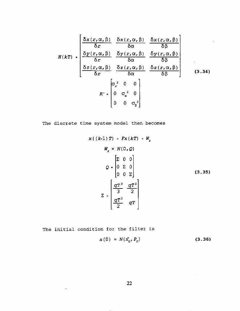
H ( k T ) =
The discrete time system model then becomes
X ( ( k + l ) T ) = F x ( k T ) + Wk
C = I-@ 2 q T
The initial condition for the filter is
x ( 0 ) = N(x^ , ,PJ
(3.34)
(3.35)
(3.36)
22

The Kalman algorithm is then given by the following set of equations
(3.37)
23

24

IV. SIMULATION RESULTS
A. OVERVIEW
The proportional navigation and CLOS simulations are tested using three target flight scenarios. In the first scenario the target has constant velocity and level flight in two dimensions. In the second, the target has a constant velocity and level flight in three dimensions. Finally, in the third, noise is added to the three-dimensional scenario.
The Simulink models and associated MATLAB code for the proportional navigation and CLOS simulations are contained in the Appendix.
B. SIMULATION ASSUMPTIONS
The following assumptions are held throughout the simulation:
(1) Acceleration due to gravity does not effect the missile or the target.
(2) The missile is lying in the xy plane at launch. (3) Missile acceleration is limited to 30g. ( 4 ) The proportional navigation constant is N = 6 .
25

C. SIMULATION SCENARIOS
1. Constant Velocity In Two Dimensions The first scenario is a two-dimensional engagement. The
target is flying at a constant altitude with no acceleration. The target parameters are as follows
X, - 30000 f t X , - -3000 ft/s xt - 0 ft/s2 yt - 0 ft y , - 0 ft/s yt - 0 ft/s2 2 , - 1000 f t 2, - 0 f t / s i; - 0 ft/s2
2. Constant Velocity In Three Dimensions The next scenario is a three-dimensional engagement. The
target is flying at a constant altitude with no acceleration. The target parameters are as follows
X, - 60000 ft X , - -2121 ft/s x t - 0 ft/s2 y, - 10000 ft y , - -2121 ft/s y, - 0 ft/s2 2 , - 1000 ft 2, - 0 ft/s 2, - 0 f t / s 2
26

3. Three-Dimensional Simulation With Radar Noise The final simulation uses the same target parameters as
the three-dimensional constant velocity simulation. White noise is added to the target flight. This simulates received noise in the target's radar return. The noise has the following characteristics
D. RESULTS AND SIMULATION COMPARISON
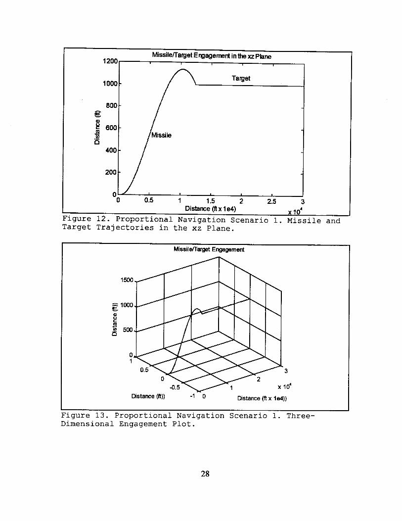
Figure 12 indicates the missile leads the target. This is attributed to the slow missile autopilot time constant
(~-=1 sec) and the target's speed advantage of mach 3 to mach
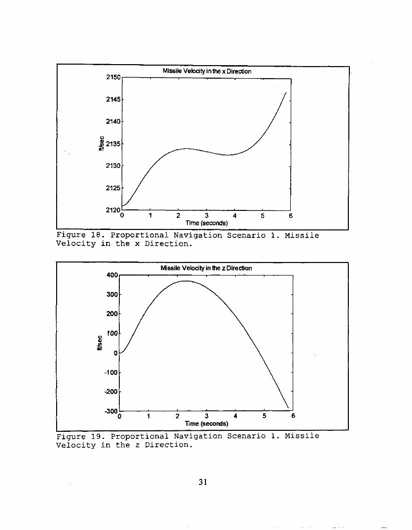
2 over the missile. This problem is exaggerated in figures 12 and 13 since the z scale is twenty times the x scale. It was determined by considering the z acceleration profile in figure 16, the z velocity profile in figure 19, and the z position profile in figure 12, that this effect was caused by the autopilot.
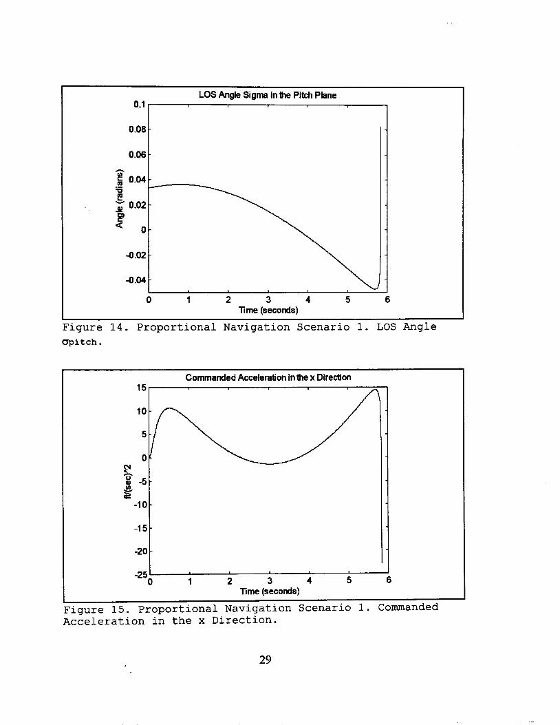
Figure 14 shows the rate of change of 0 is positive for
approximately 1 second; thereafter it is negative but, for 2
seconds the missile has a positive commanded acceleration. Figures 15 and 16 show the missile's acceleration variations. Figures 17, 18 and 19 show the missile's velocity variations.
27
Missilemarget Engagement in the xz Plane
12001------ 1000 -
800 - n s k! 600- # 5
400 -
200 - / 0 0 0.5 1 1.5 2 2.5 3
x lo4 Distance (ft x 1 e4) Figure 12. Proportional Navigation Scenario 1. Missile and Target Trajectories in the xz Plane.
Missilmarget Engagement
Distance (ft)) -1 0 Distance (ft x 1 e4))
Figure 13. Proportional Navigation Scenario 1. Three- Dimensional Engagement Plot.
28
0.08
0.06 h
0.04
L
0 -
0.02 -
0 .a
-
-
-
I t \ I w ,
Figure 14. Proportional Navigation Scenario 1. LOS Angle dpitch.
Commanded Acceleration inlhe x Direction 15
1 2 3 4 5 6 -25 I 0
lime (seconds)
Figure 15. Proportional Navigation Scenario 1. Commanded Acceleration in the x Direction.
29
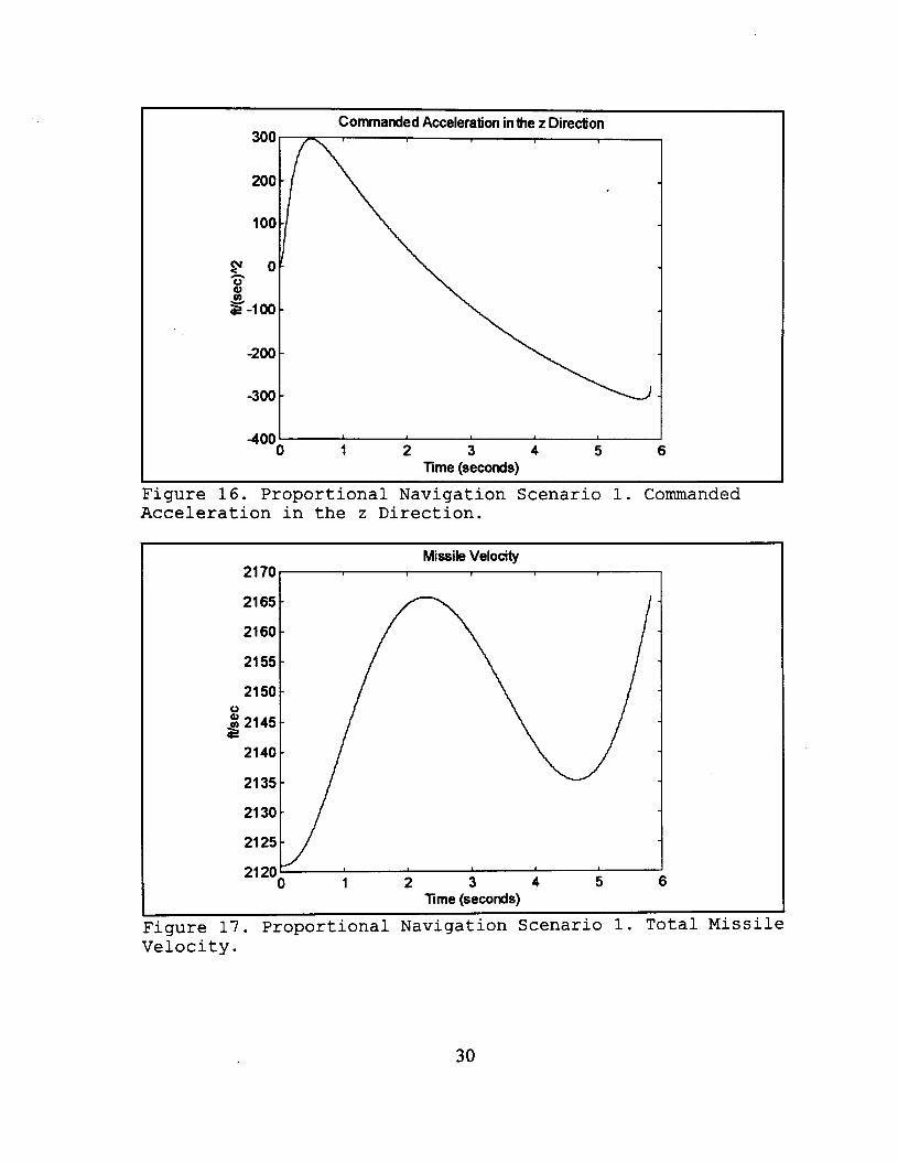
Figure 16. Proportional Navigation Scenario 1. Commanded Acceleration in the z Direction.
Missile Velocity 21 70
21 65 1 2160 t 21 55 1 21 50
0
2145
21401
21 21351 30
21 25 1
1 2 3 4 5 6 21 20 0
Time (seconds)
Figure 17. Proportional Navigation Scenario 1. Total Missile Velocity.
30
Missile Velocity inthe x Direction 21501 I
2145
I
1 2 3 4 5 6 2120;
Time (seconds)
Figure 18. Proportional Navigation Scenario 1. Missile Velocity in the x Direction.
Missile Velocity in the z Direction 400 1
1 2 3 4 5 6 -300 '
0 Time (seconds)
Figure 19. Proportional Navigation Scenario 1. Missile Velocity in the z Direction.
31

Plots for the other scenarios are given in the Appendix. The following table summarizes the missile's closest point of approach (CPA), and the time of the CPA for each simulation.
Scenario
1
2
3
Simulation CPA Time of CPA
Prop Nav 4.13 ft 5.89 s
CLOS 1.39 ft 7.18 s
Prop Nav 14.94 ft 14.72 s
CLOS 1.24 ft 19.51 s
Prop Nav 27.15 ft 14.5 s
CLOS 267.79 ft 22.34 s
Overall, the proportional navigation missile achieves a quicker target intercept time. The miss distances for each missile are very close, except when noise is added. The CLOS missile degrades significantly in the presence of noise.
The proportional navigation missile is a superior missile. The CLOS missile is unable to give satisfactory results when sensor noise is added to the simulation. For very short range intercept scenarios, where sensor noise is negligible, the missile will perform well. The proportional navigation missile will perform well for any engagement scenario. This fact makes proportional navigation preferable for missile guidance.
32
V. CONCLUSIONS AND RECOMMENDATIONS
A. CONCLUSIONS
The simulation provides insight in chosing the proper type of missile guidance. The two types of guidance explored both give acceptable miss distances without sensor noise. However, when sensor noise is present the proportional navigation missile outperformed the CLOS missile.
The presence of an on board seeker gives the proportional navigation missile an advantage when dealing with sensor noise. Since the sensor is on the missile as it closes the target, the sensor noise will have less of an effect on the detection of the target. The CLOS missile is guided from a stationary radar at the launch site. The error incurred from sensor noise does not decrease as the missile approaches the target. To overcome this problem the CLOS missile will require a very sophisticated tracking radar that has very little sensor noise.
The addition of noise to the engagement provides a more realistic scenario for the missile control problem. Developing a noise filter and adjusting the missile characteristics to adapt to the noise created a unique and educational challenge. The increased realism reinforced the fact that actual missile control developement is a compromise of design requirements.
B . RECOMMENDATIONS
The simulation can be taken to several different levels. The target flight can be modified for different engagement scenarios. A manuevering target would provide another level of realism to the engagement.
An adjoint model could be built for each simulation.
33

This would aid in the miss distance analysis for the two
missiles. Finally, different noise filters can be developed and
tested. The miss distance will be decreased if better noise filtering is achieved during the simulation.
34
APPENDIX
A. COMMAND GUIDED MISSILE PLOTS FOR SCENARIO 1
n
E.
d a !! v)
1200
1000
800
600
400
200
Missileflarget Engagement in the xz Plane I I I I I
Target
i ssi le -
I I I I I
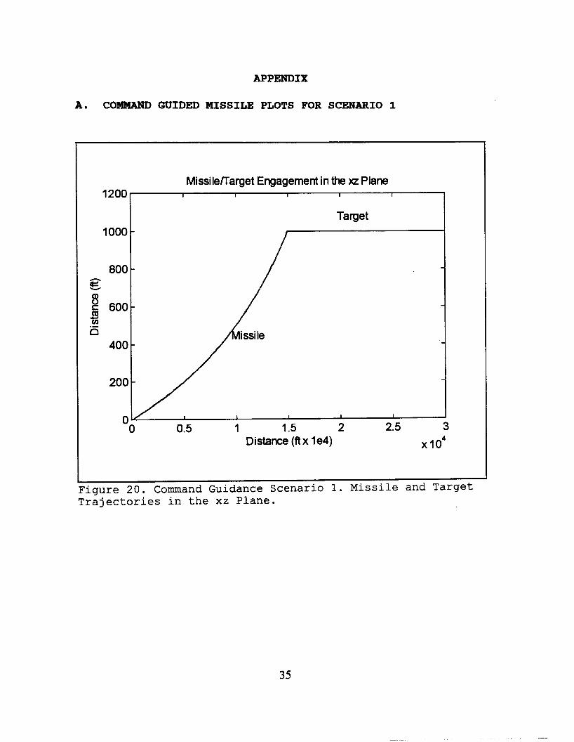
0 0.5 I 1.5 2 2.5 3 Distance (ft x 1 e4) x 104
Figure 20. Command Guidance Scenario 1. Missile and Target Trajectories in the xz Plane.
35
Missile Target Engagement
Distance (feet x 1 e4) Distance (feet) -1 0
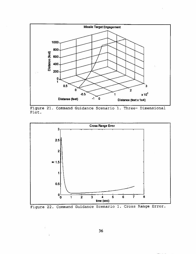
Figure 21. Command Guidance Scenario 1. Three- Dimensional Plot.
Cross Range Error
3w
time (sec)
Figure 22. Command Guidance Scenario 1. Cross Range Error.
36
Commanded Acceleration in the x Direction
. .
10
0
-1 0
-20
-60
-70
-80 I
1 2 3 4 5 6 7 8 -90
0 time (sec)
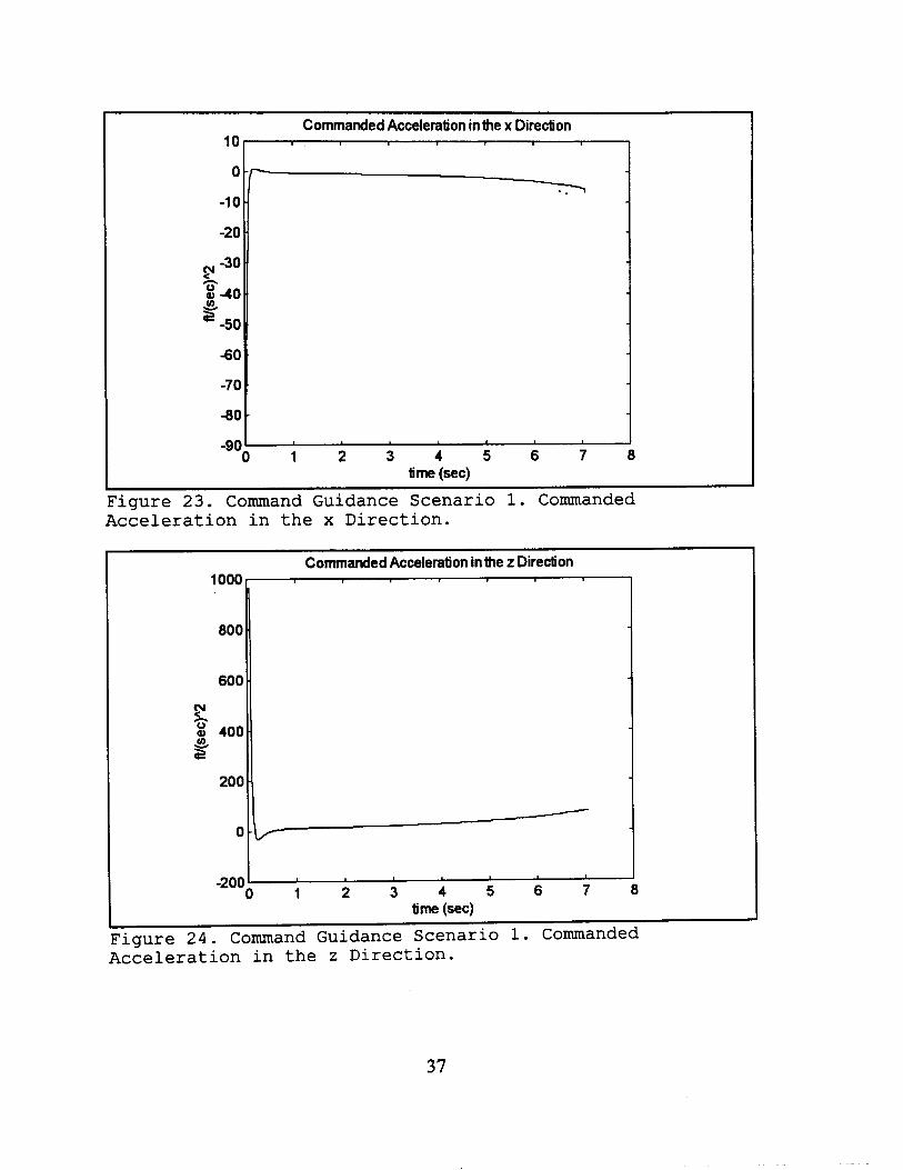
Figure 23. Command Guidance Scenario 1. Commanded Acceleration in the x Direction.
commanded Acceleration in the z Direction 1000
800
600
$11,
f 8 400
200
37
Missile Velocity 21 25
2118.
21 16
g2114-
$2112-
2110-
2108
2106
21 04
21 211gl 18
-- -
-
2124 -
2123 -
2122 -
2121 -
2120 -
21 24
21 23
21 22
21 21
21 20
21 19
21 18
21 17' 0 1 2 3 4 5 6 7 8
time (sec)
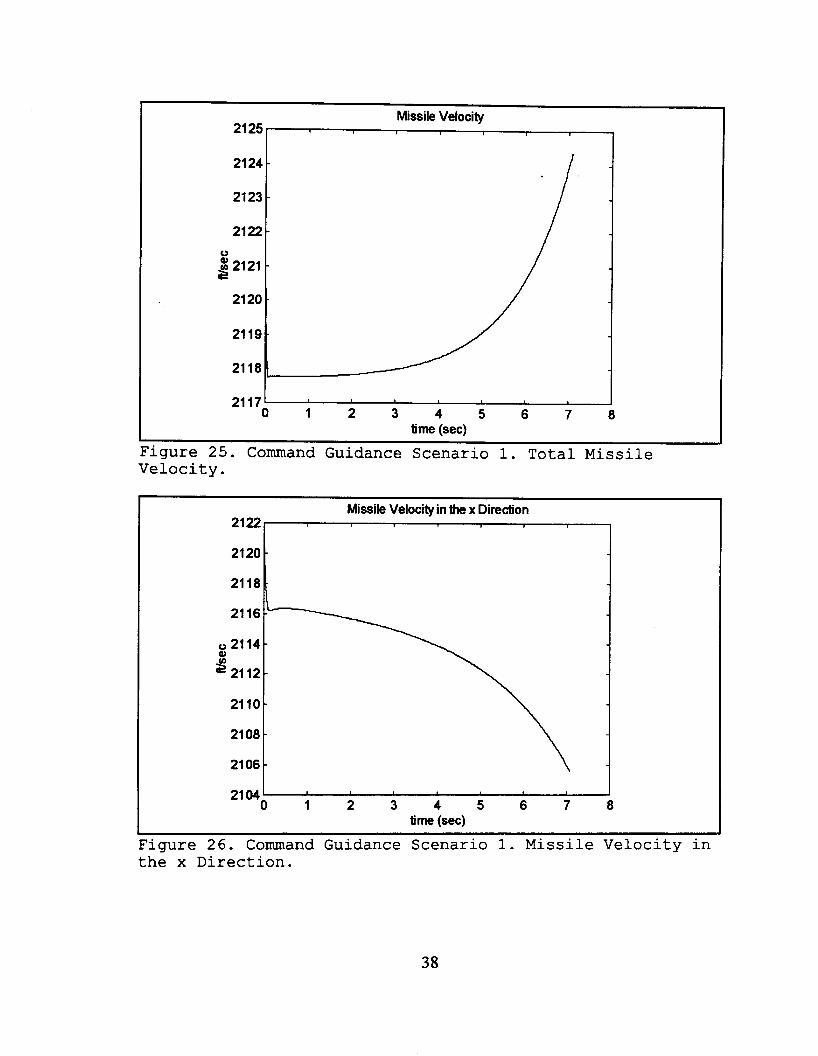
Figure 25. Command Guidance Scenario 1. Total Missile Velocity .
38
300
250
200
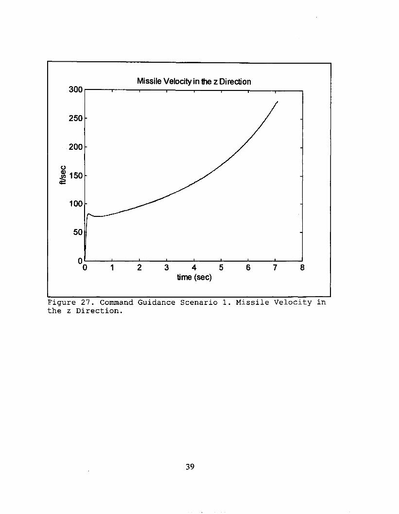
Missile Velocity in the z Direction I 1 I I I I I
0' I I I I I I I
0 1 2 3 4 5 6 7 8 time (sec)
Figure 27. Command Guidance Scenario 1. Missile Velocity in the z Direction.
39
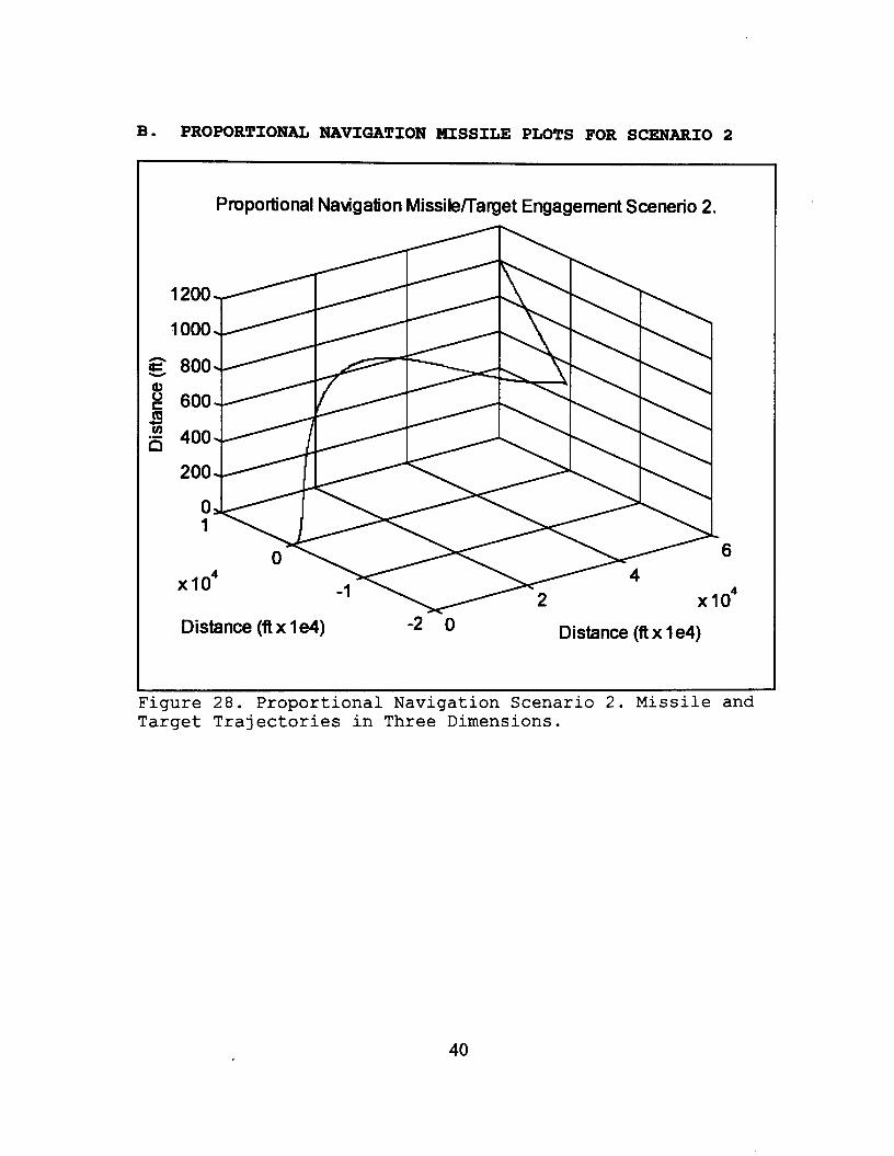
B. PROPORTIONAL NAVIGATION MISSILE PLOTS FOR SCENARIO 2
Proportional Navigation Missilenarget Engagement Scenerio 2.
Distance (ft x 1 e4) Distance (ft x 1 e4) -2 -0
Figure 28. Proportional Navigation Scenario 2. Missile and Target Trajectories in Three Dimensions.
40
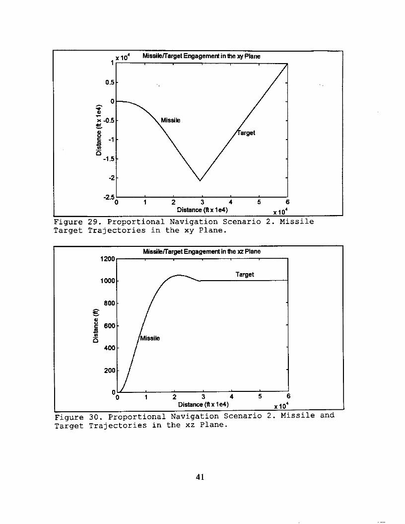
Figure 29. Proportional Navigation Scenario 2. Missile Target Trajectories in the xy Plane.
800
E
c W Z 600-
a 400
200
-
-
-
1 000 1 Target
1 Distance (ft x 1 e4)
Figure 3 0 . Proportional Navigation Scenario 2. Missile and Target Trajectories in the xz Plane.
x l o 4
41

I x lo4 Distance (ft x 1 e4)
Figure 31. Proportional Navigation Scenario 2. Missile Target Trajectories in the yz Plane.
LOS Angle Sigma in the Pitch Plane 025 r
I
-0.05; 5 10 15 Time (sec)
Figure 32. Proportional Navigation Scenario 2. LOS Angle Qpitch.
42
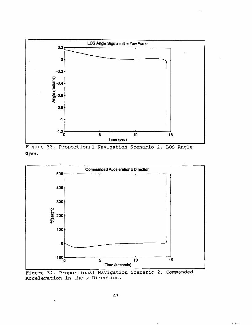
LOS Angle Sigma in the Yaw Plane
400
300
g-0.6
-0.8
-
-
Tme (sec)
Figure 33. Proportional Navigation Scenario 2. LOS Angle dyaw .
100
Commanded Acceleration x Direction 500 I
-
O\
8 200 f
43
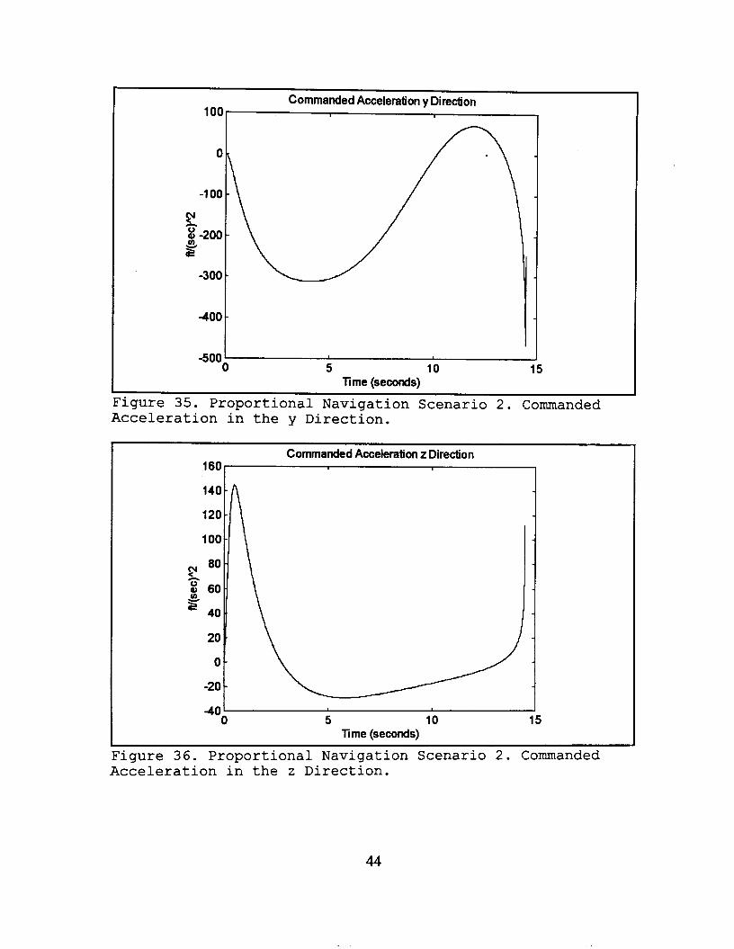
Commanded Acceleration y Direction 1001
5 10 lime (seconds)
15
Figure 35. Proportional Navigation Scenario 2. Commanded Acceleration in the y Direction.
I 160
140
120
100
80
8 60 ' 40
E!
20
0
-20
4 0 0
commanded Acceleration z Direction
5 10 15
I Time (seconds)
Figure 36. Proportional Navigation Scenario 2. Commanded Acceleration in the z Direction.
44
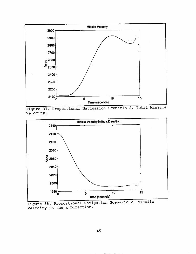
3000
2900
2800
2700
8 2600
2500
2400
2300
2200
21 00
Time fseconds)
-
-
-
-
-
-
-
5 10 15
21 40
21 20
J
Ve ioci t y .
21001
20801 0
2060
2040 t 2000 2020 t
Time (seconds)
Figure 38. Proportional Navigation Scenario 2. Missile Velocity in the x Direction.
45
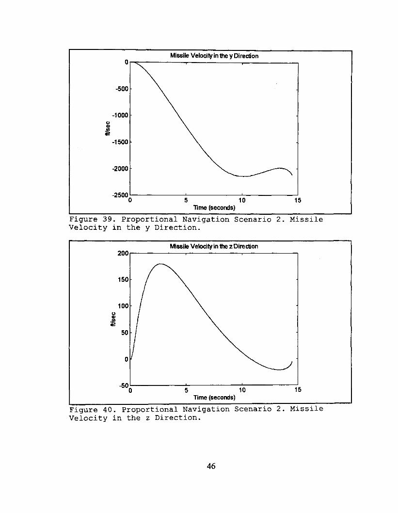
0
-500
-1 000
-1 500
-2000
-2500 0
Missile Velocity in the y Direction
5 10 Time (seconds)
15
Figure 39. Proportional Navigation Scenario 2. Missile Velocity in the y Direction.
Figure 40. Proportional Navigation Scenario 2. Missile Velocity in the z Direction.
46
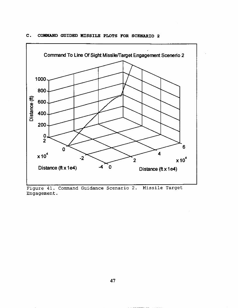
C. COMMAND GUIDED MISSILE PLOTS FOR SCENARIO 2
Command To Line Of Sight Missilemarget Engagement Scenerio 2
Distance (ft x 1 e4) 4 0 Distance (ft x 1 e4)
~~~ ~
Figure 41. Command Guidance Scenario 2. Missile Target Engagement.
47
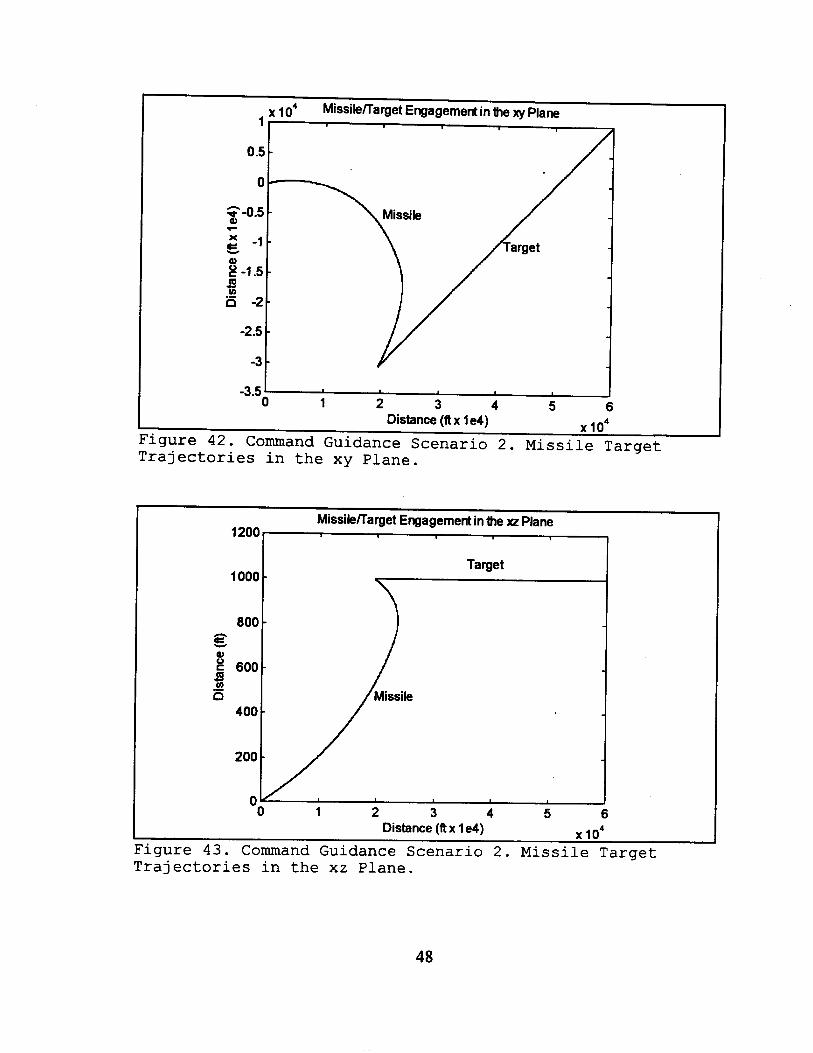
I l o 4 Distance (ft x 1 e4) Figure 4 2 . Command Guidance Scenario 2 . Missile Target T r a j e c t o r i e s i n t h e xy Plane.
MissileEarget Engagement in the xz Plane
1200r----- 1000 -
800 - E
# Q)
2 600-
6 400 -
200 -
Target
0 1 2 3 4 5 6 Distance (ft x 1 e4) - .,4 x I U
Figure 4 3 . Command Guidance Scenario 2 . Missile Target T r a j e c t o r i e s i n t he xz Plane.
48
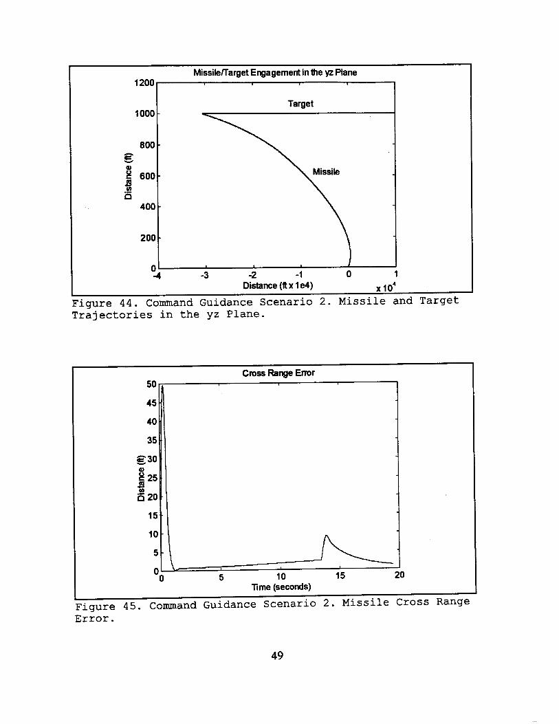
1200
1000
800
E
+! 0
2 600-
6 400
200
0 -
Error.
Target -
-
-
-
49
0.8
50
40
30 !5
E 20 # 6
i o
a
n
0)
-1 c
0.7
0.6
0.5 h s g 0.4
# 0.3 ii
c
0 2
0.1
0
Cross Range Error in the Pitch Plane
t
5 10 15 20 -0.1
0 Time (seconds)
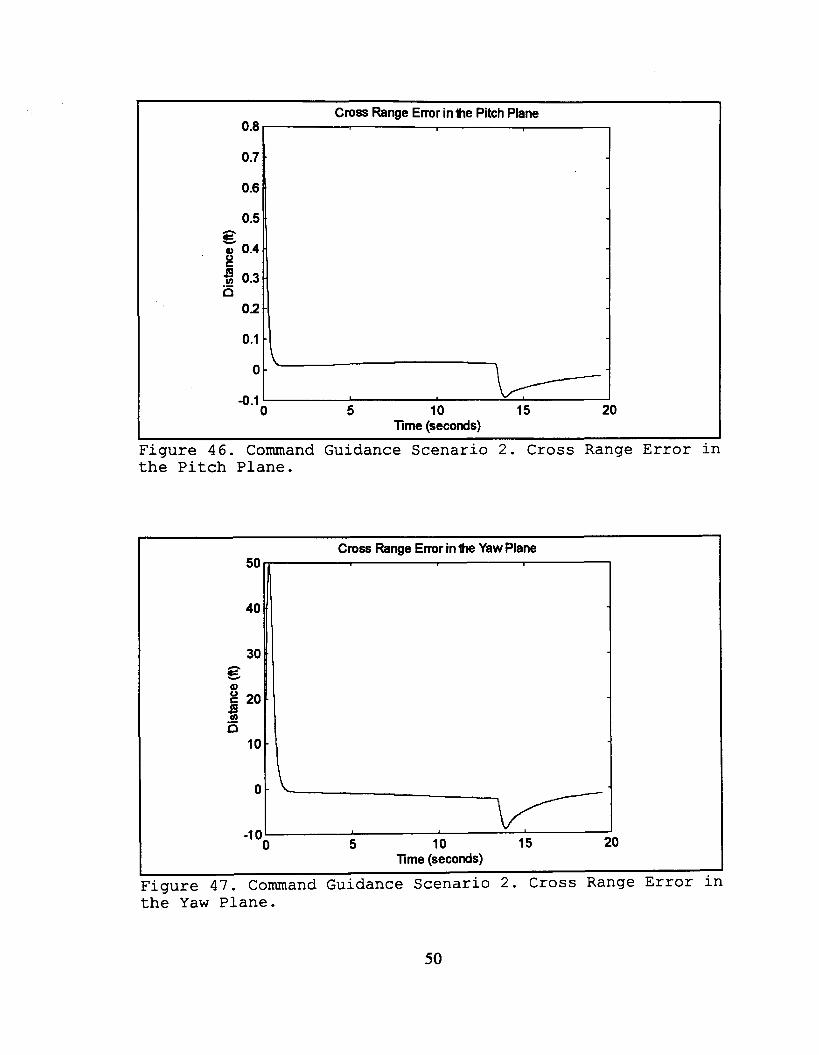
Figure 46. Command Guidance Scenario 2. Cross Range Error in the Pitch Plane.
Cross Range Error in the Yaw Plane
Time (seconds)
the Yaw Plane.
50
Commanded Acceleration in the x Direction 200 r
0 -
-200.
r 8 -400.
600
-800
-1 000 0 5 10 15 20 Time (seconds)
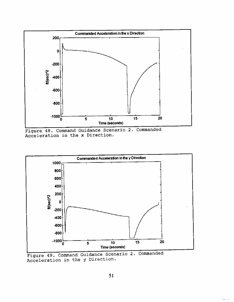
Commanded Acceleration in the y Direction 1000 - 800 -
600 -
400 - 200 -
8 0 - r 3
-200-
-400 - -600 -
-800 -
0 5 10 15 20 -1 000
Time (seconds)
51
Commanded Acceleration in the z Direction
l o o 0 c
600 8oo t
-200 ' 0 5 10 15 20
Time (seconds)
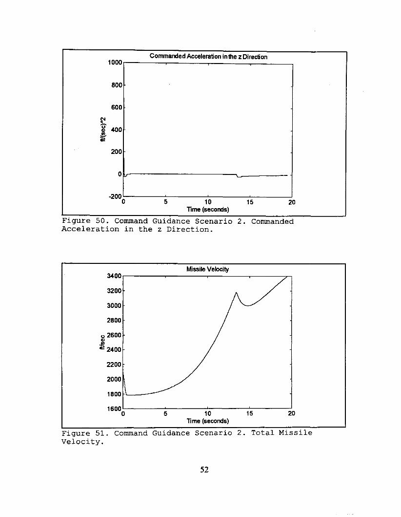
Figure 50. Command Guidance Scenario 2. Commanded Acceleration in the z Direction.
3400
3200
3000
2800
0 2600 Q, ' 2400
2200
2000
Missile Velocity
0 5 10 15 20 Time (seconds)
1600
Figure 51. Command Guidance Scenario 2. Total Missile Velocity.
52

Missile Velocity in the x Direction 2500
Missile Velocity in the x Direction 2500
2000 \ 1500 -
1000 - 0 500-
6 0 -
-500 -
-1000 -
-1 500 -
-2000 0 5 10 15 20
Time (seconds)
-2000 ' 0 5 10 15 20
Time (seconds)
Figure 52. Command Guidance Scenario 2. Missile Velocity in the x Direction.
Missile Velocity in the y Direction 500
-1000 - 0
-2000 -
-2500 -
0 5 10 15 20 Time (seconds)
Figure 53. Command Guidance Scenario 2. Missile Velocity in the y Direction.
53
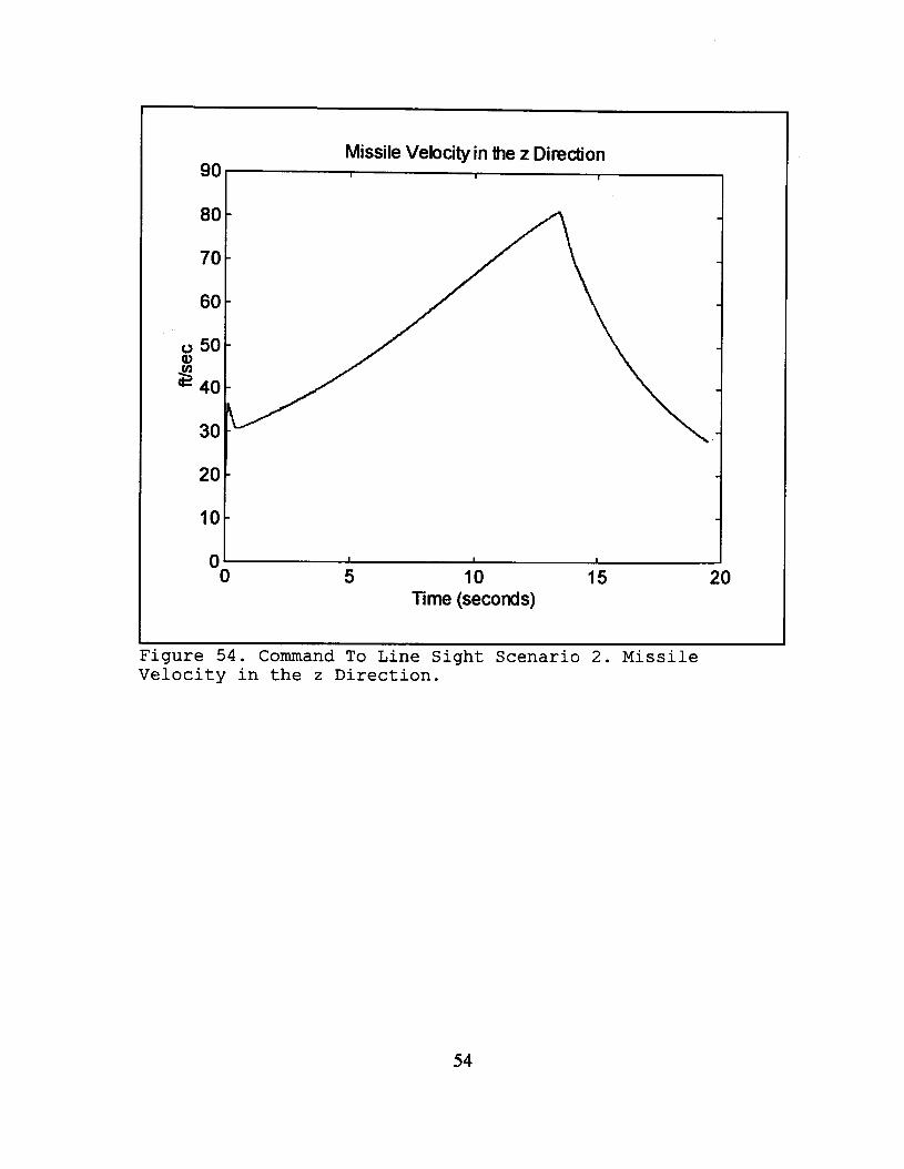
Figure 54. Command To Line Sight Scenario 2. Missile Velocity in the z Direction.
54

D. PROPORTIONAL NAVIGATION MISSILE PLOTS FOR SCENARIO 3
Missile Target Engagement
Distance (ft x 1 e4) Distance (ft x 1 e4) - 4 0
Figure 55. Proportional Navigation Scenario 3 . Missile and Actual Target Trajectory.
55
Missile Target Engagement
n
!5 Q) 1000 - 0 c= Q 3 500- - 0
0 I I I
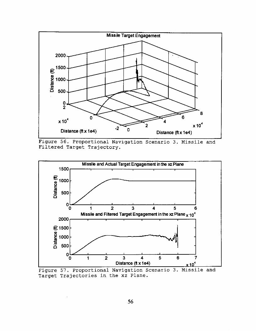
Figure 56. Proportional Navigation Scenario 3. Missile and Filtered Target Trajectory.
2000 - 1 I I I I 1
1500 - - 0 2 1000- - c v) 5 500- -
I 0
56
04 Missile and Actual Target Engagement in the xy Plane
1500
e - 1000 2
ii
al
Q 500-
0 1 2 3 4 5 6
I I I I I I
-
-
I I 1 I
104 Missile and Filtered Target Engagement in the xy Plane 1 o4 n 2 I I I I I 1 .4 al
- al - c v)
ii 4. I I I I I I
0 1 2 3 4 5 6 7 Distance (a x 1 e4) 4
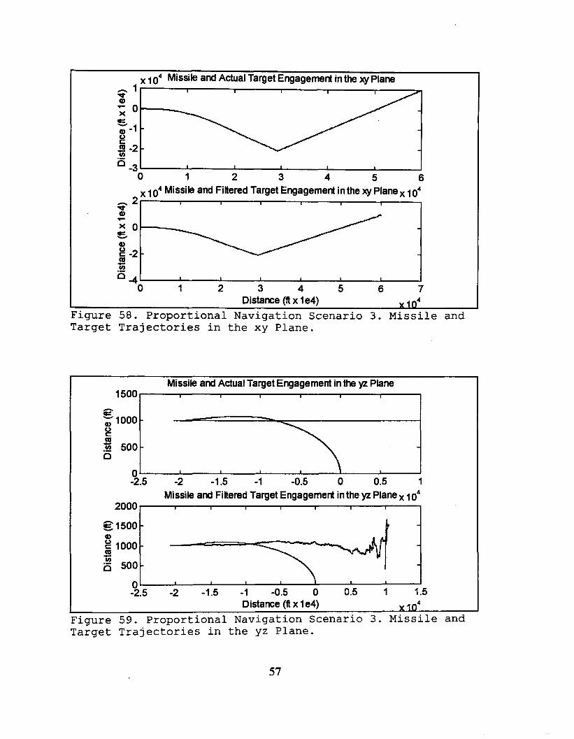
'igure 58. Proportional Navigation Scenario 3. Missile and Target Trajectories in the xy Plane.

I 2900 t
2 8 0 3
2800 t
I 1
-
t I
2700 t 8 2600
2500
2400 t 2300 1 22001
21 00 0 5 10 15
Time (sec) . . Figure 60. Proportional Navigation Scenario 3. Total Missile Ve 1 oci t y .
58
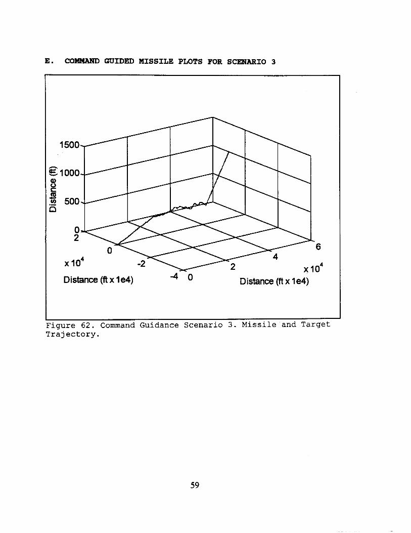
E. COMMAND GUIDED MISSILE PLOTS FOR SCENARIO 3
Distance (ft x le4) - 4 0 Distance (ft x 1 e4)
Figure 62. Command Guidance Scenario 3 . Missile and Target Trajectory.
59
d Q) r
x 0- E. 8 s -2 i i 4 4 v)
I I I
- -
Distance (ft x 1 e4) 4
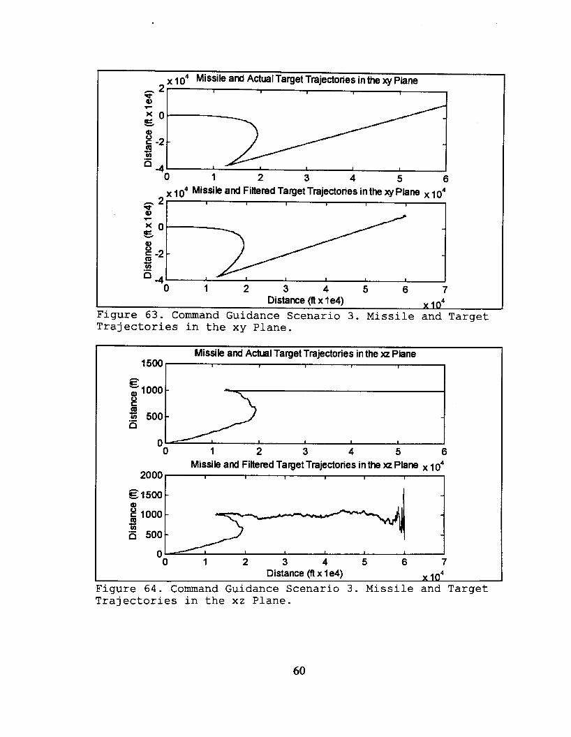
Figure 63. Command Guidance Scenario 3. Missile and Target Trajectories in the xy Plane.
* Q) r -
-
n
slooo - 8
6
c 0
500-
0
-
I I I I
60
E l 5 0 0 - - 1000 - - 500- -
c
0- I
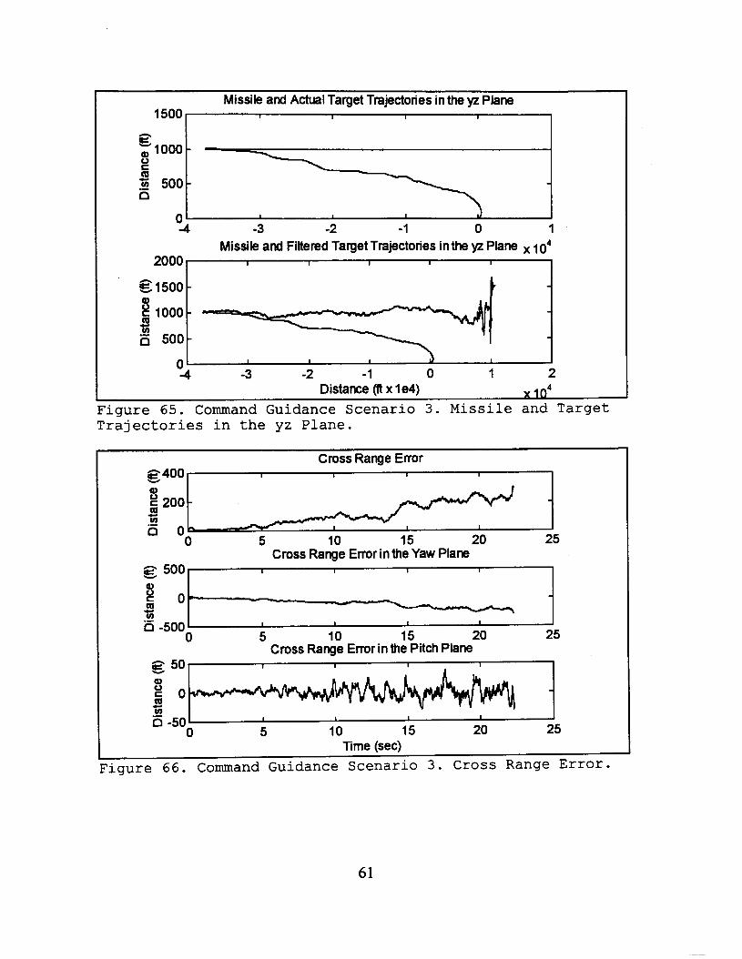
Missile and Actual Target Trajectories in the 'yz Plane
n 5 1000 - 2 3 500- - a
E l 5 0 0 - r -
3 c! 1000 - -
500- -
Distance (ft x 1 e4) 4
Figure 65. Command Guidance Scenario 3. Missile and Target T r a j e c t o r i e s i n t h e y z Plane.
Cross Range Error
T g 400
E 200 c u)
0 5 10 15 20 25 a 0 Cross Range Error in the Yaw Plane
0 c 5 u) -500 50:: 0 5 10 15 20 25
- Cross Range Error in the Pitch Plane
I I I I I 0 5 10 15 20 25
Time (sec)
Figure 66 . Command Guidance Scenario 3. Cross Range Er ro r .
61
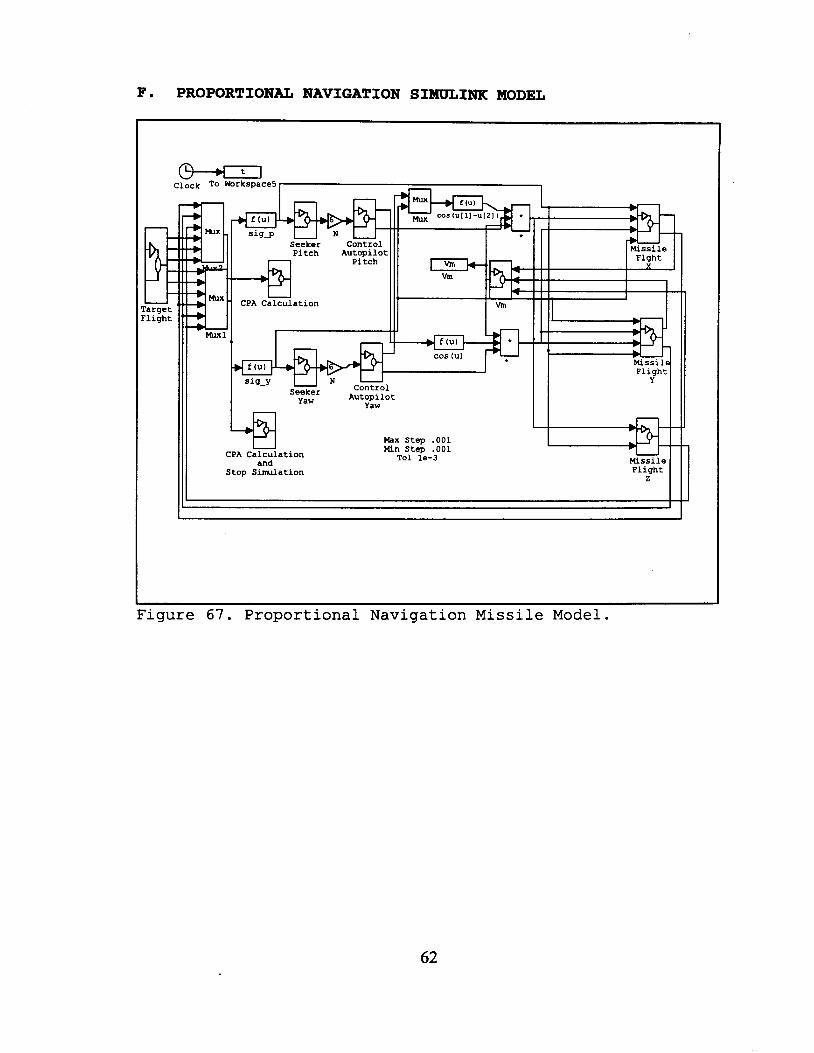
F. PROPORTIONAL NAVIGATION SIMULINK MODEL
CPA Calculation and
Stop Simulation
CPA Calculation
I 1 - - N -
Control Autopilot
Yaw
Seeker Yaw
Clock To Workspace5
Max Step .001 Min Step .001
To1 le-3
Flight Y
I - I I
Missile Flight
z
Figure 67. Proportional Navigation Missile Model.
62
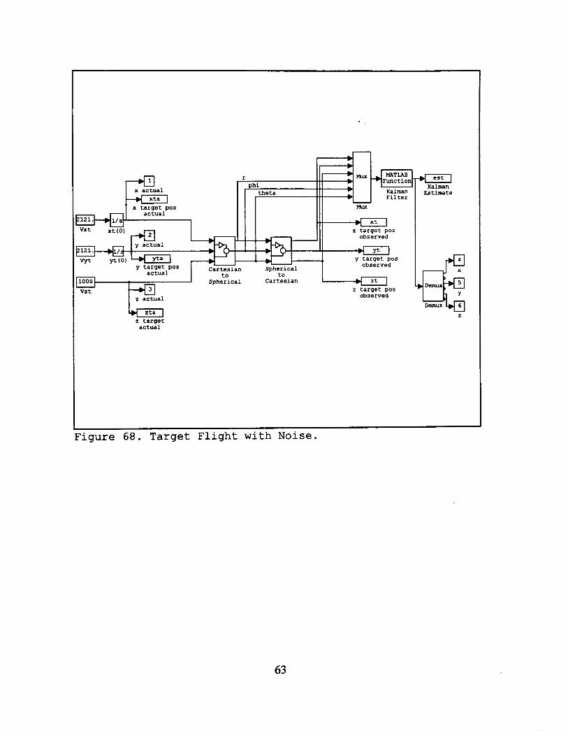
x actual Lk, x target pos
y target pos
z actual
z target actual
observed
to Cartesian
z target pos observed
Estimate
7igure 68. Target Flight with Noise.
63
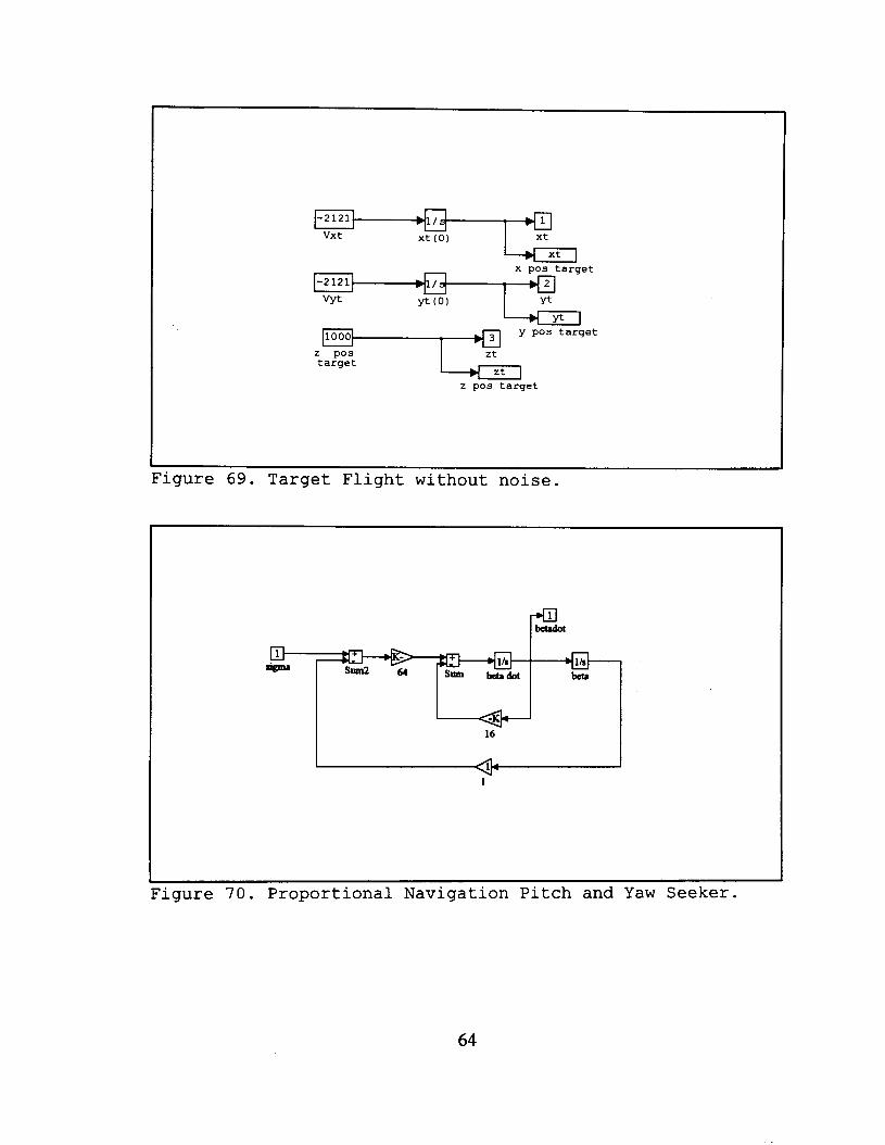
-2121 1 v x t xt l a
x pos target
Yt
1 a y pos target
z PO3 target
2 pos target
Figure 69. Target Flight without noise.
b
Figure 70. Proportional Navigation Pitch and Yaw Seeker.
v- 1
64
gammadot
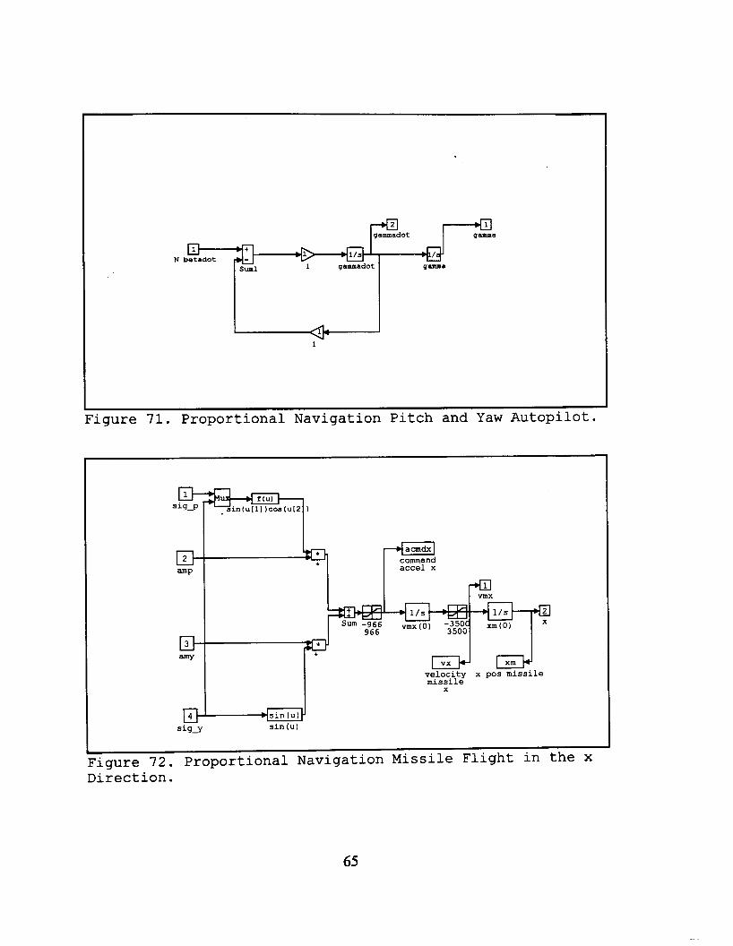
I 1
Figure 71. Proportional Navigation Pitch and Yaw Autopilot.
command I accel x
X
VmX
velocity x pos missile missile
65
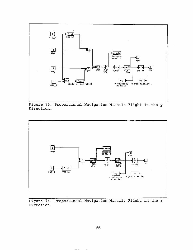
Figure 7 3 . Proportional Navigation Missile Flight in the y Direction.
accel z
f (u) s i g g cos(u)
velocitv z pos missile missile -
Figure 74. Proportional Navigation Missile Flight in the z Direction.
66
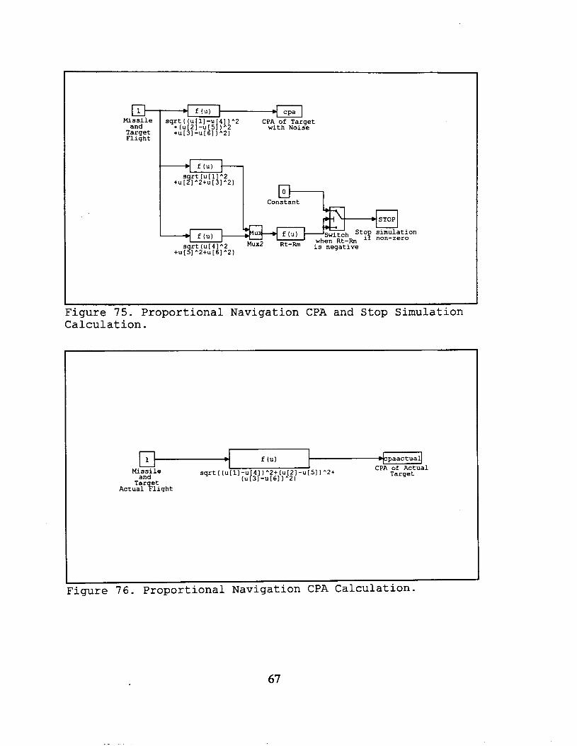
Missile and
Target Flight
f (u) Sqrt((u[ll-u[41)^2 CPA of Target
with Noise
Constant - Figure 75. Proportional Navigation CPA and Stop Simulation Calculation.
Figure 76. Proportional Navigation CPA Calculation.
- 1 f (u)
(~[31-u161)"2) CPA of Actual
Target Missile sqrt ( (u[ll -u 141 "2+ (u [21-u 151 ^2+ and Tar et
Actual %light
67
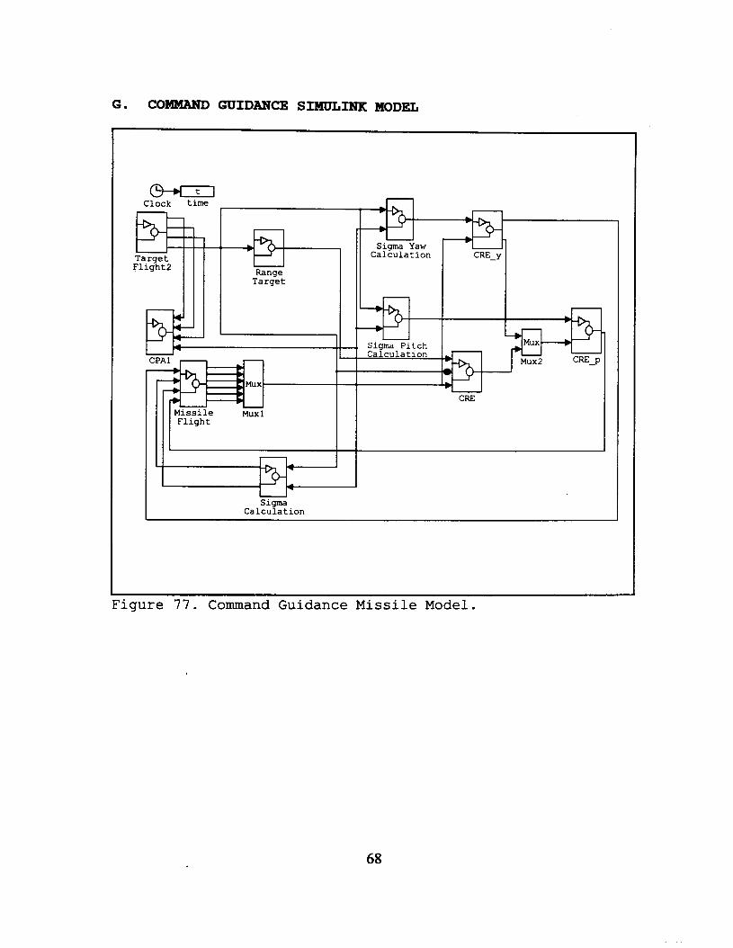
G . COMM?WD GUIDANCE SIMULINK MODEL
Clock time . b
r-+
- - b
+
I k I
sigma Yaw Calculation
UI’
Flight
-- CREJ
_ ,
I I
Sigma Calculation
Sigma Pitch Calculation
+-
1
CRE
Figure 77. Command Guidance Missile Model.
68
target
Vxt Xt(0)
1000 b
Zt I I b
E-
I-’ l r M A T F
- Filter
Function Kalman
- b b
M u x Dhl
eta
Hux
r - b b
M u x Dhl
Ka - Fi
II I I I I Hux I
rt z position target
z position target with
noise
estimated target position
4 Target observed flight
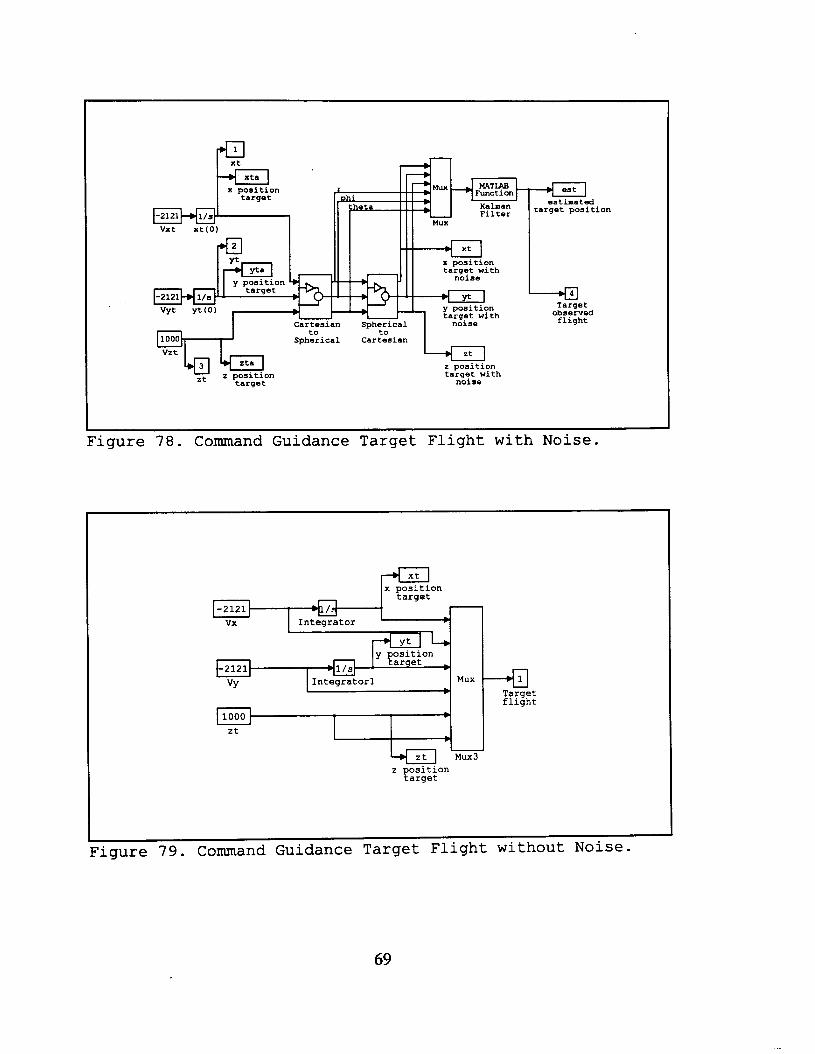
Figure 78. Command Guidance Target Flight with Noise.
target
flight -
U Mux3
z position target
69
F velocity
I
ll
7 accel z
-czl veloci tv
Y
+J y positi missilt Vy
k
1 crep Demux cepdot &+, z position
missile velocity
2
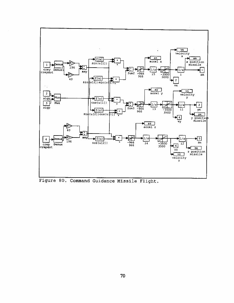
Figure 80. Command Guidance Missile Flight.
70
- 1 . f (u) I
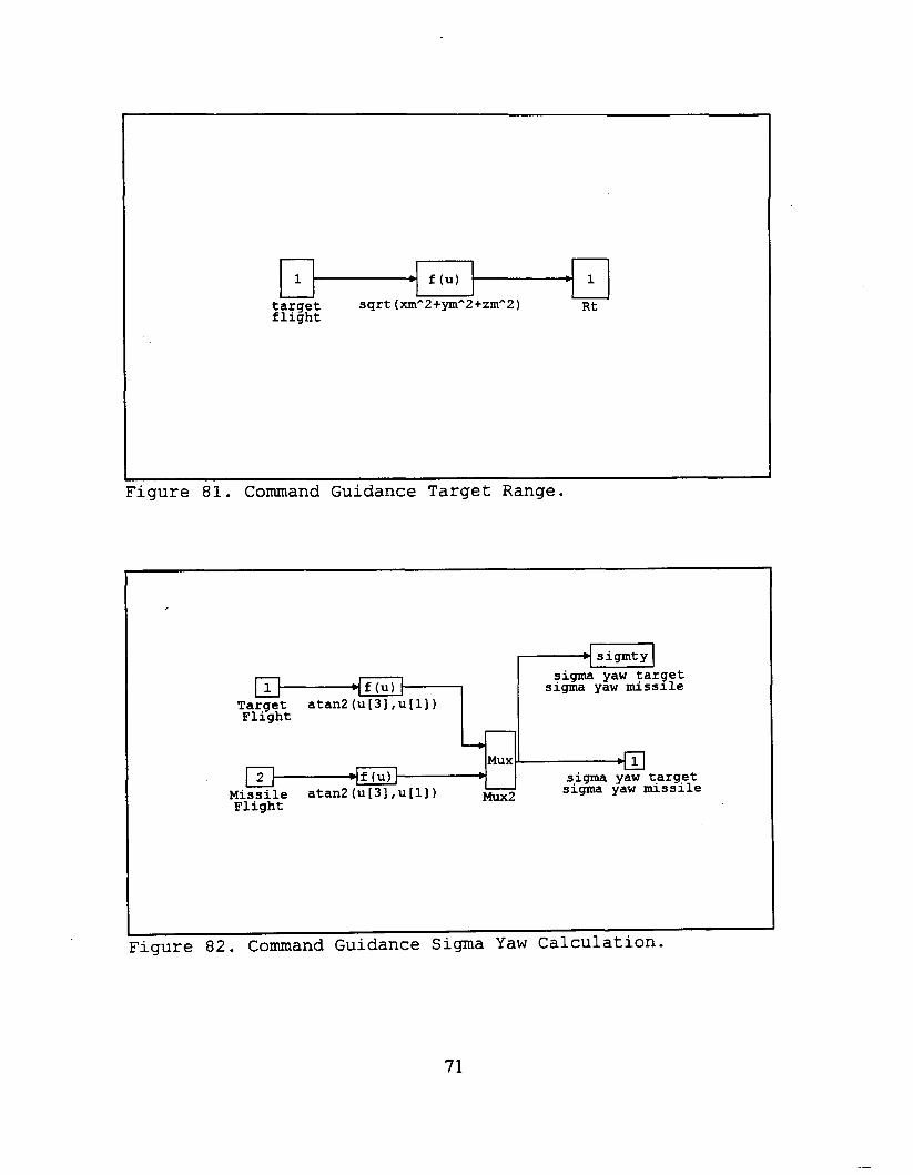
Figure 81. Command Guidance Target Range.
- b 1
r
sigma yaw target sigma yaw nussile
Target atan2 (u[31 , u [ l l ) Flight
Mux 1 2 s.igma yaw tprget - sigma yaw missile
Missile atan2 (ut31 ,u[ll) Mux2 Flight

- f(u) b
Figure 83. Command Guidance Sigma Pitch Calculation.
sigmtp sigma pitch target sigma pitch missile
Figure 84. Command Guidance Sigma Calculation.
target flight
atan2 (u[51 ,sqrt (u[11A2+u[31 -2 j )
.
Mux -
b Demux 4 S i 9 Y 1 , Demuxl
sigma t Yaw target
atan2 ( (u [2] -u [ 61 ) , (u [ 11 -u [ 41 ) ) sigma Yaw
* 4 sigp I _*
b
., + Mux * b
sigma pitch
Demux ~ atan2 ( (u [3]-u[E] ) , sigma ~qrt ( (u[ 11-u 141 ) "2+ ( U C21-U [ G I ) ̂ 2) pitch missile A
Mux Demux
72

target flight Demuxl'
Figure 85. Command Guidance Cross Range E r r o r .
Cross l/u Range Error
Rt 1/Rt
- a -b * Cross
--* Range Error
- .
b
missile
I - b Mux - ere yaw f ( u )
qigma yaw t,arg,et sin(u[l]-u[21 I Muxl credot yaw sigma yaw missile
, sqrt ( (ymzt-ytzm) ̂2+ (xtzm-xmzt) "2+
Demux , (xmyt-xtym) ̂2)
Figure 86 . Command Guidance Cross Range Error Y a w .
73
- sigma- pitch missile
CRE pitch r MUXI credot pitch
crepd CREdot pitch Derivative
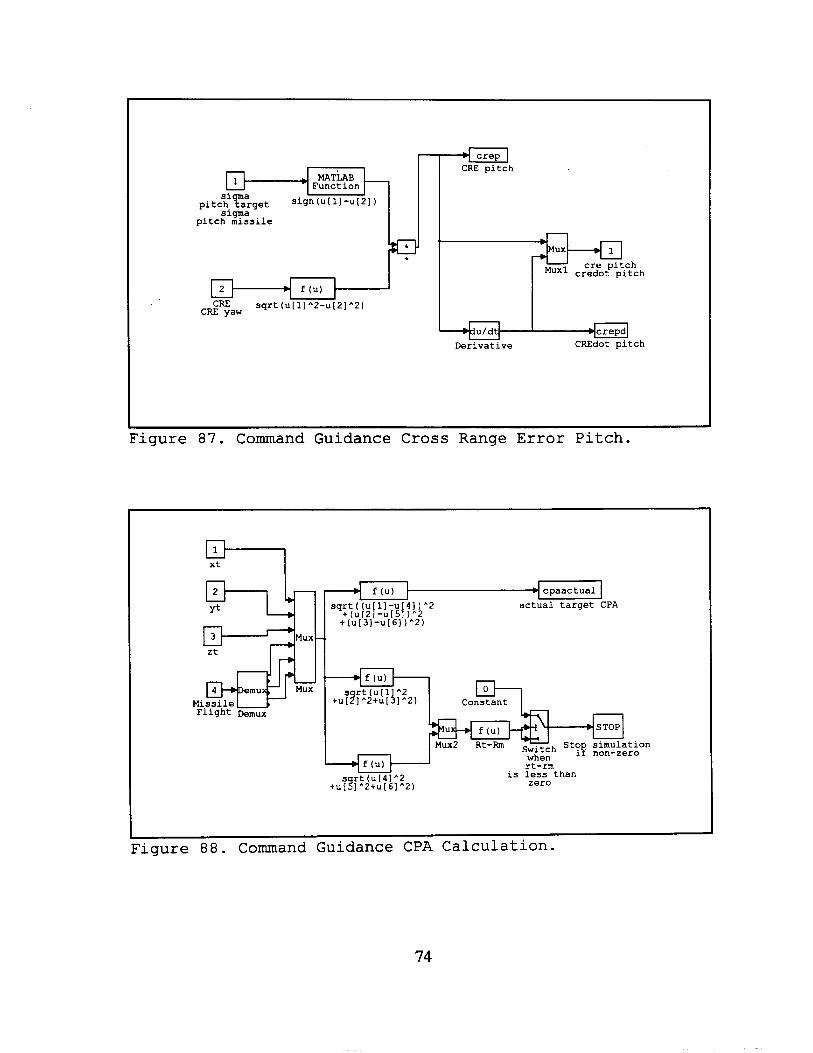
Figure 87. Command Guidance Cross Range Error Pitch.
cpaactual f (u)
t(u[21-u[51)^2 +(u[31-~[61)"2)
sqrt((u[ll-u[41)"2 actual target CPA
.
is less than zero
I Figure 88. Command Guidance CPA Calculation.
74
I I I
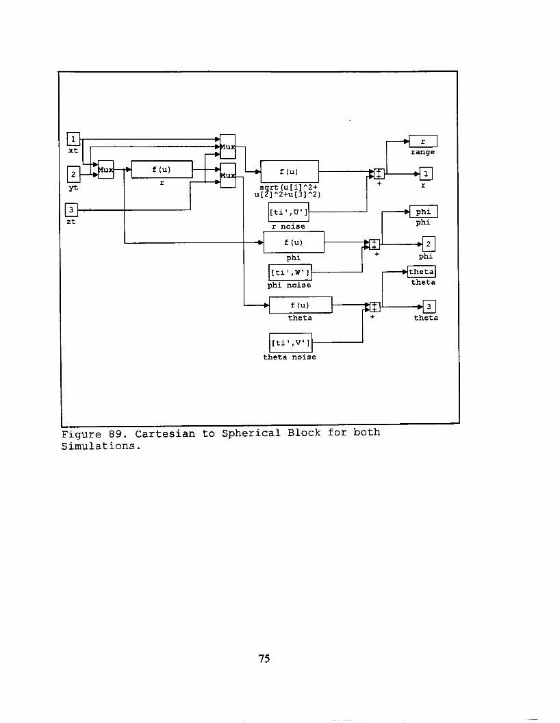
theta + theta
[ti',V']
theta noise
I Figure 89. Cartesian to Spherical Block f o r both Simulations.
75

H. MISCELLANEOUS MATLAB CODE
% This program generates the noise used in the target flight. randn ( seed ,26 57 9 ) ; ti=[O: .001:30]; for i= 1:30001 %Range noise U(i) = randn*i5;
%Pitch angle noise V(i) = randn*pi/l80;
%Yaw angle Noise W(i) = randn*pi/l80;
end %This program sets the initial conditions for the Kalman %Filter. It is run at the beginning of each simulation. clear P clear xhat global P global xhat %initial covariance matrix P=le6 *eye (6 ) ;
%initial estimated target position xhat=[10000 -500 1000 -500 0 5001';
%This function runs a Kalman filter algorithm %for the given A , B, C matices for constant velocity flight function[xhat,P] =klmn(u,P,xhat) ; %initialization A = [ O 1 0 0 0 0 ;
0 0 0 0 0 0 ;
0 0 0 1 0 0 ;
0 0 0 0 0 0 ;
0 0 0 0 0 1 ;
76
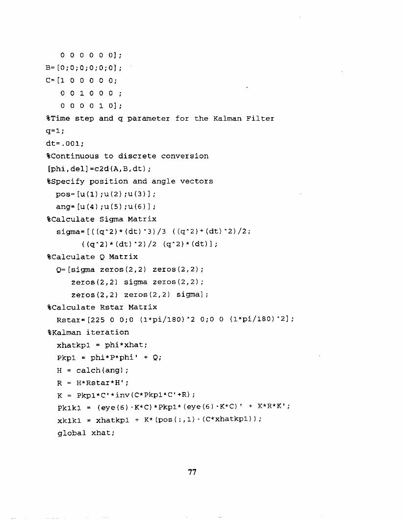
0 0 0 0 0 01;
B=[O;O;O;O;O;O] ;
C=[1 0 0 0 0 0 ; 0 0 1 0 0 0 ;
0 0 0 0 1 0 1 ;
%Time step and q parameter for the Kalman Filter q=l; dt= .001; %Continuous to discrete conversion [phi,dell =c2d(A,B,dt) ; %Specify position and angle vectors
pos= [u(1) ;u(2) ;u(3) 1 ; ang= W 4 ) ;u(5) ;u(6) 1 ;
%Calculate Sigma Matrix sigma=[((qA2)*(dt)^3)/3 ((qA2)*(dt)"2)/2;
( (q-2) * (dt) "2) /2 (q-2) * (dt) 1 ; %Calculate Q Matrix
Q= [sigma zeros(2,2) zeros(2,2) ; zeros(2,2) sigma zeros(2,2) ; zeros(2,2) zeros(2,2) sigma] ;
%Calculate Rstar Matrix Rstar= [225 0 0;O (1*pi/180) -2 0 ; O 0 (l*pi/180) -21 ;
%Kalman iteration xhatkpl = phi*xhat; Pkpl = phi*P*phi' + Q;
H = calch(ang1; R = H*Rstar*H'; K = Pkpl*C'*inv(C*Pkpl*C'+R) ;
Pkikl = (eye(6) -K*C)*Pkpl* (eye(6) -K*C) + K*R*K'; xklkl = xhatkpl + K* (pos ( : ,1) - (C*xhatkpl) ) ; global xhat;
77
.. .
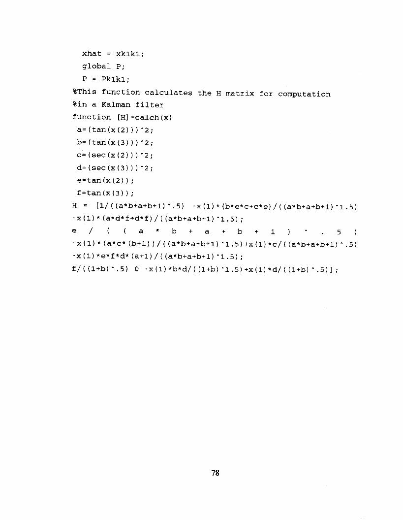
xhat = xklkl; global P;
P = Pklkl; %This function calculates the H matrix for %in a Kalman filter function [HI =calch(x) a=(tan(x(2)) 1-2; b=(tan(x(3)))^2;
c= ( sec (x (2 ) -2 ;
d= (sec (x (3 ) ) -2 ;
e=tan(x(2)) ; f=tan(x(3)) ;
computation
H = [I/( (a*b+a+b+l) -.5) -x(l)* (b*e*c+c*e)/( (a*b+a+b+l) -1.5) -x(l)* (a*d*f+d*f)/( (a*b+a+b+l) -1.5) ;
e / ( ( a * b + a + b + i ) ^ - 5 ) -x(l)*(a*c*(b+l))/((a*b+a+b+l) A1.5)+x(i)*c/((a*b+a+b+i)A.5)
-x(l)*e*f*d* (a+l)/( (a*b+a+b+l) -1.5) ;
f / ( (I+b) A .5 ) 0 -X (1) *b*d/ ( (I+b) -1.5 ) +X (1) *d/ ( (I+b) A . 5 ) ] ;
78
BIBLIOGRAPHY
Blackelock, J.H., A u t o m a t i c Control o f A i r c r a f t and Missiles, Wiley-Interscience Publishing, New York, NY. 1991.
Davis, H.F., I n t r o d u c t i o n t o Vector A n a l y s i s , Wm.C. Brown Publishing, Dubuque, IA. 1991.
Hostetter, G.H., Santana, M.S., Stubberud, A.R., D i g i t a l Control System Des ign , Saunders College Publishing, Fort Worth, TX. 1994.
Peppas, D.1, "A Computer Analysis of Proportional Navigation and Command to Line of Sight of a Command Guided Missile for a Point Defence System," M.S. Thesis, Naval Postgraduate School, Monterey CA, December 1992.
Titus, H.A., Missile Guidance, unpublished notes, Naval Postgraduate School, Monterey, CA.
79

80
INITIAL DISTRIBUTION LIST
1. Defense Technical Information Center Cameron Station Alexandria, Virginia 22304-6145
2. Library, Code 52 Naval Postrgaduate School Monterey, California 93943-5101
No. Copies 2
3. Chairman, Code EC Department of Electrical and Computer Engineering Naval Postgraduate School Monterey, California 93943-5121
4. Professor H.A. Titus, Code EC/Ts Department of Electrical and Computer Engineering Naval Postgraduate School Monterey, California 93943 -5121
5. Professor R.G. Hutchins, Code EC/HU Department of Electrical and Computer Engineering Naval Postgraduate School Monterey, California 93943-5121
6. Professor P. Pace, Code EC/Pc Department of Electrical and Computer Engineering Naval Postgraduate School Monterey, California 93943-5121
7. Lieutenant Patrick Costello 9 Rhonda Dr. Scarborough, Maine 04074
2
1
1
1
1
1
81